Minimal flux Minkowski classification

Niall T. Macpherson and Alessandro Tomasiello

Dipartimento di Fisica, Università di Milano–Bicocca,
Piazza della Scienza 3, I-20126 Milano, Italy
and
INFN, sezione di Milano–Bicocca

niall.macpherson@mib.infn.it, alessandro.tomasiello@unimib.it
Abstract

We classify Minkowski₄ solutions in type IIA supergravity, with ${\cal N}=2$ supersymmetry and an SU(2) R-symmetry of a certain type. Many subcases can be reduced to relatively simple PDEs, among which we recover various intersecting brane systems, and AdS_d solutions, $d=5,6,7$, and in particular the recently found general massive AdS₇ solutions. Imposing compactness of the internal six-manifold we obtain promising solutions with localized D-branes and O-planes.

1 Introduction

String theory compactifications become harder to find as the cosmological constant of the spacetime factor increases. There are many known families of AdS examples ($\Lambda<0$); the oldest known type is the Freund–Rubin class [1] which has a Sasaki–Einstein as internal space, but many other possibilities have been found over the years.

Finding de Sitter examples ($\Lambda>0$) is infamously much harder. Several no-go results [2, 3, 4] imply that this is only possible at the cost of including quantum corrections and/or orientifold sources. Supersymmetry has to be broken in this case, which is of course to be expected at some scale anyway, but which makes finding such solutions harder.

For Minkowski solutions $(\Lambda=0)$, supersymmetry can still be preserved. One expects intuitively this case to be much rarer than AdS already because setting $\Lambda=0$ looks like fine-tuning. Indeed the de Sitter no-go theorems in supergravity [2, 3, 4] also apply here, with the only exception of solutions where the metric is the only non-zero field. In this case the internal space has to be Ricci-flat. For compactifications of type II supergravity to four dimensions, these are Calabi–Yau manifolds. These exist in large numbers, and their study has been very fruitful to string theory and to geometry. But a more general study of Minkowski solutions can be useful both as a laboratory for string theory dynamics and as intermediate construction for the $\Lambda>0$ case.

To add the other supergravity fields, the antisymmetric fields often called “fluxes”, one obvious possibility is to add D-branes: a probe analysis shows that these can be wrapped on complex or special Lagrangian cycles of the Calabi–Yau while preserving half of the supercharges. The Bianchi identity shows that one also has to add O-planes, in agreement with the general no-go theorems. One expects that the backreaction of these objects should then distort the internal metric. In general these metrics, while expected to exist, are not easy to exhibit explicitly (after all the Calabi–Yau metrics themselves are not known). For the special case of D3–O3 configurations, the distortion treats all the internal coordinates in the same way, and one ends up with a conformally Calabi–Yau $M_{6}$. Remarkably, one can also add a combination of three-form fluxes (as long as they are $(2,1)$ and primitive) without breaking supersymmetry [5, 6, 7, 8]. However, these solutions are still based on modifications of the Calabi–Yau geometry.

In full generality, supersymmetry imposes [9] that the internal $M_{6}$ should be a so-called “generalized Calabi–Yau” [10, 11] with extra conditions involving the fluxes. Still, explicit examples where all these conditions are met are hard to obtain. Since several generalized Calabi–Yau’s have been found, it is natural to start from those and to try to impose the extra flux conditions on them. One can obtain a few formal solutions in this way [12], but they rely on the presence of sources which are smeared all over $M_{6}$: this can be fine for D-branes, but not for O-planes, which are not dynamical and should sit at fixed loci of involutions. One can hope that such formal solutions are an “approximation” to more sensible ones where the sources are localized, but this needs to be demonstrated case by case.

More sophisticated attempt have been made. For example [17] looked for solutions with localized sources on solvmanifolds in bigger generality than in [12], finding examples again when the internal space is Ricci-flat. [18] recently looked at an Ansatz inspired by the conformal Calabi–Yau class [5, 6, 7, 8] and proved some general results. Impressively, [19, 20] used a mix of generalized complex geometric and algebraic geometric methods to produce U-fold Minkowski₄ solutions.

In this paper we take a different approach. Rather than making an Ansatz on the type of internal geometry or topology, we choose a broad class, and we let supersymmetry fix the internal geometry. This can succeed because, in some situations, there are enough internal spinors so that their bilinears can define an entire vielbein (in this context, an “identity structure”). While this phenomenon has been known for a long time, it has become clearer in recent times that the local metrics thus naturally chosen by supersymmetry often tend to have automatically the correct behaviors one would expect from O-planes and D-branes. For example, AdS₇ solutions naturally allow for localized O6-sources [21], and the same is true for their AdS₄ cousins obtained by twisted compactification [22]. Since, as we mentioned, O-planes are essential for Minkowski compactifications, it feels natural to apply to them as well this “identity structure” approach.

We thus analyze systematically a broad class of solutions, defined by its type of supersymmetry rather than by the internal topology. The class we chose lies at the intersection of several already existing physical constructions. It is rich enough for the classification to be interesting, and yet constrained enough for it to be very detailed. It consists of solutions with ${\cal N}=2$ unbroken supersymmetry, which admit an SU(2) R-symmetry acting in the simplest way, namely on an $S^{2}$ factor. We assumed the presence of the R-symmetry so as to allow us to recover various AdS_d solutions with $d=5,6,7$; in particular the AdS₇ solutions recently obtained in massive IIA [21, 23] and the M-theory AdS₅ solutions of [24]. (This latter point suggests that our results should be useful to look for ${\cal N}=2$ solutions in massive IIA as well.)

Within our class, we reduce the classification to three broad subclasses (see figure 1 below for a visual summary). Within each, preserved supersymmetry can be reduced to a system of PDEs; sometimes further sub-subclasses suggest themselves, and within each the PDEs simplify considerably. Some of these systems have appeared earlier in the literature for intersecting brane solutions [25, 26, 27]. In fact the local form of the metric formally resembles in many cases that of a brane or of a brane system. One of the three subclasses is T-dual in its entirety to the conformal Calabi–Yau solutions [5, 6, 7, 8].

We will also illustrate the classification with some examples. As we already mentioned, we recovered several classes of AdS_d solutions, $d=5,6,7$. We also studied the case where $M_{6}$ is compact. Even for the PDE systems that were already postulated in the literature for intersecting branes, this had not been really attempted. We will find a couple of workable examples; in particular one with an O6 and an ONS5. More work is required for a more thorough understanding of the various possibilities offered by our results.

In section 2 we introduce our Ansatz. After some preliminary work in section 3 about the pure spinor formalism we use, we give our detailed classification in section 4, with a summary in section 4.6. We conclude with examples in section 5.

Note added. While this work was being completed, [28] appeared, which has some overlap with our section 5.2 about recovering AdS₇ solutions.

2 The Ansatz

In this section, we will motivate and introduce our Ansatz. We are looking for ${\cal N}=2$ Mink₄ solutions with an SU(2) R-symmetry acting on an $S^{2}$ factor.

As is customary we take the metric to be a warped product

$$ds^{2}_{10}=e^{2A}ds^{2}_{{\rm Mink}_{4}}+ds^{2}_{6}$$ (2.1)

with the warping function $A$, the dilaton $\phi$ and the NS 3-form $H$ depending on the internal space $M_{6}$ only. The RR fluxes decompose as

$$F_{\rm tot}=\sum_{k=0}^{5}F_{2k}=f+e^{4A}\text{Vol}_{4}\wedge\star_{6}\lambda(f),$$ (2.2)

where $f$ denotes the total internal RR flux. The function $\lambda$ acts on an arbitrary $n$-form as $\lambda(\alpha_{n})=(-1)^{\frac{n}{2}(n-1)}\alpha_{n}$ which ensures the higher and lower forms are related as $F_{n}=(-1)^{\frac{n}{2}(n-1)}\star_{10}F_{10-n}$. The Bianchi identities and equations of motion for the RR fluxes collectively read, away from any localised sources:

$$d_{H}F_{\rm tot}=0\,,\qquad d_{H}=d-H\wedge\,.$$ (2.3)

The $d_{H}\star_{6}\lambda(f)$ part of this follows from supersymmetry, while the $d_{H}f$ part needs to be imposed. The equation of motion for the three-form $H$ was also proven [29] to follow from the supersymmetry equations, so we will not write it here.

The supersymmetry parameters for an ${\cal N}=2$ solution with flux in general read

$$\begin{split}&\epsilon_{1}=\sum_{a=1}^{2}\zeta^{a}_{+}\otimes\chi_{1+}^{a}+\text{c.c.}\\ &\epsilon_{2}=\sum_{a=1}^{2}\zeta^{a}_{+}\otimes\chi_{2-}^{a}+\text{c.c.}\end{split}$$ (2.4)

where $\zeta$ and $\chi$ denote spinors on Mink₄ and $M_{6}$ respectively. (We define $(\zeta_{+})^{c}=\zeta_{-}$, $(\chi_{b+}^{a})^{c}=\chi_{b-}^{a}$, $b=1,2$.) We make the reasonable simplifying assumption that the spinors on $M_{6}$ have equal norm. This is a global requirement for the existence of AdS_d solutions in $d=4,5,6,7$ and a local one for the existence of D-brane or O-plane sources, but is not needed in full generality.

Minkowski solutions don’t necessarily have an R-symmetry. Eventually, however, we would like to apply our results to AdS_d solutions with $d>4$. Indeed for example AdS₅ solutions can be viewed as Mink₄ solutions by taking in (2.1)

$$e^{A}=e^{A_{5}+\rho}\ ,\qquad ds^{2}_{6}=e^{2A_{5}}d\rho^{2}+ds^{2}_{5}\ .$$ (2.5)

For AdS solutions R-symmetry has to be present: this is ultimately because it is necessarily a part of the superconformal algebra, even though it is optional in supersymmetry. In particular, AdS solutions with eight supercharges have an SU(2) R-symmetry.

Thus we will assume the existence of an SU(2) R-symmetry. It will act on $M_{6}$ as an isometry. We will assume that it acts on $S^{2}$ leaves of a foliation on $M_{6}$. In other words, the metric will locally factorize as $S^{2}\times M_{4}$, with the radius of the $S^{2}$ depending on the coordinates on $M_{4}$ (including the possibility of shrinking to zero at some loci). This is what we will call the “minimal” class. It is not a priori the most general situation: one might take $M_{4}$ to be topologically fibred over $S^{2}$, for example with $M_{6}=M_{3}\times$ a squashed $S^{3}$.

In this situation, the spinor Ansatz needs to be refined from the general (2.4). The $\zeta^{a}$ are a doublet under SU(2)_R; thus we also need a doublet of spinors $\xi^{a}$ in the internal space, so that the ten-dimensional $\epsilon_{1,2}$ are invariant. In fact, since SU(2)_R acts only on the $S^{2}$, the $\xi^{a}$ need to transform as a doublet under the isometry group of $S^{2}$. Such a doublet is given by the so-called Killing spinors on $S^{2}$, which is also related to its Killing vectors. It is of the form

$$\xi^{a}=\left(\begin{array}[]{c}\xi\\ \xi^{c}\end{array}\right)\ ;$$ (2.6)

see appendix A for details.

We can also play with chirality projections, to obtain doublets $\zeta^{a}_{\pm}$ and $\xi^{a}_{\pm}$ on Mink₄ and $S^{2}$ respectively. So there are four possible SU(2)_R singlets; this leads us to

$$\begin{split}\epsilon_{1}&=\sum_{a=1}^{2}\zeta^{a}_{+}\otimes\xi^{a}_{+}\otimes\eta^{1}_{+}+\zeta^{a}_{+}\otimes\xi^{a}_{-}\otimes\eta^{1}_{-}+\zeta^{a}_{-}\otimes\xi^{a}_{-}\otimes\tilde{\eta}^{1}_{+}+\zeta^{a}_{-}\otimes\xi^{a}_{+}\otimes\tilde{\eta}^{1}_{-}+\text{c.c.},\\ \epsilon_{2}&=\sum_{a=1}^{2}\zeta^{a}_{+}\otimes\xi^{a}_{+}\otimes\eta^{2}_{-}+\zeta^{a}_{+}\otimes\xi^{a}_{-}\otimes\eta^{2}_{+}+\zeta^{a}_{-}\otimes\xi^{a}_{-}\otimes\tilde{\eta}^{2}_{-}+\zeta^{a}_{-}\otimes\xi^{a}_{+}\otimes\tilde{\eta}^{2}_{+}+\text{c.c},\end{split}$$ (2.7)

where the $\eta^{a}$, $\tilde{\eta}^{a}$ are now spinors on $M_{4}$. When one writes out the supersymmetry equations, however, one actually realizes the $\eta$’s and $\tilde{\eta}$’s never mix. Thus including the $\tilde{\eta}$’s only gives more constraints, beyond those that are necessary for minimal supersymmetry in four dimensions, and not a generalization; we can then set them to zero without loss of generality. So we are left with

$$\begin{split}\epsilon_{1}&=\sum_{a=1}^{2}\zeta^{a}_{+}\otimes\xi^{a}_{+}\otimes\eta^{1}_{+}+\zeta^{a}_{+}\otimes\xi^{a}_{-}\otimes\eta^{1}_{-}+\text{c.c.},\\ \epsilon_{2}&=\sum_{a=1}^{2}\zeta^{a}_{+}\otimes\xi^{a}_{+}\otimes\eta^{2}_{-}+\zeta^{a}_{+}\otimes\xi^{a}_{-}\otimes\eta^{2}_{+}+\text{c.c}.\end{split}$$ (2.8)

One of the first condition one encounters when working with (2.7) is that the norms of the $\chi_{b}^{a}$ should be proportional to $e^{A}$ [12, App. A.3]. For SU(2)_R to be unbroken, one needs this to be independent of the coordinates on $S^{2}$; which implies

$$||\eta^{a}_{+}||^{2}=||\eta^{a}_{-}||^{2}\ .$$ (2.9)

In the rest of the paper, we will classify “minimal” solutions using (2.8) as a starting point. As we will see, the geometry is already constrained enough that a very detailed classification is possible; this is ultimately due to the fact that the internal spinors $\chi^{a}_{b}$ define an identity structure.

3 Pure spinors

Having described our “minimal” class of manifolds, we will now classify its solutions. We will use the pure spinor formalism [9], with our precise conversions .

First of all, there is no need for us to consider all the $\chi^{a}_{b}$. If we impose that an ${\cal N}=1$ subalgebra is preserved (corresponding for example to the $\chi_{b}\equiv\chi_{b}^{1}$), R-symmetry will imply automatically that the second set of supercharges is also preserved. So we can simply work with the two internal spinors

$$\begin{split}\chi^{1}_{+}&=e^{\frac{A}{2}}(\xi_{+}\otimes\eta^{1}_{+}+\xi_{-}\otimes\eta^{1}_{-}),\\ \chi^{2}_{-}&=e^{\frac{A}{2}}(\xi_{+}\otimes\eta^{2}_{-}+\xi_{-}\otimes\eta^{2}_{+})\ .\end{split}$$ (3.1)

If we define the bispinors

$$\Phi_{-}=e^{-A}\chi^{1}_{+}\otimes\chi^{2{\dagger}}_{-}\ ,\qquad\Phi_{+}=e^{-A}\chi^{1}_{+}\otimes\overline{\chi}^{2}_{-},$$ (3.2)

where $\overline{\chi}=(\chi^{c})^{{\dagger}}$, the differential forms associated to them via the Clifford map are pure spinors for the Cl$(6,6)$ algebra living on the “generalized tangent bundle” $T\oplus T^{*}$. Preserved supersymmetry is equivalent to the following “pure spinor equations” [9] on $M_{6}$:

$$d_{H}\left(e^{3A-\Phi}\Phi_{+}\right) =0,$$ (3.3a)

$$d_{H}\left(e^{2A-\Phi}\text{Re}\Phi_{-}\right) =0,$$ (3.3b)

$$d_{H}\left(e^{4A-\Phi}\text{Im}\Phi_{-}\right) =\frac{e^{4A}}{8}\star_{6}\lambda(f),$$ (3.3c)

where $\lambda(f)=\lambda(f_{0}+f_{2}+f_{4}+f_{6})=f_{0}-f_{2}+f_{4}-f_{6}$.

The decomposition (3.1) induces a decomposition of the pure spinors $\Phi_{\pm}$; this can be used to reduce the system (3.3) to one on $M_{4}$. One can define

$$\begin{split}&\Psi=\eta^{1}\otimes\eta^{2{\dagger}}\ ,\qquad\tilde{\Psi}=\eta^{1}\otimes\overline{\eta}^{2},\\ &\Psi_{\hat{\gamma}}=(\hat{\gamma}\eta^{1})\otimes\eta^{2{\dagger}}\ ,\qquad\tilde{\Psi}_{\hat{\gamma}}=(\hat{\gamma}\eta^{1})\otimes\overline{\eta}^{2}\ ,.\end{split}$$ (3.4)

where $\eta^{i}=\eta^{i}_{+}+\eta^{i}_{-}$ and $\hat{\gamma}$ is the chiral gamma in $M_{4}$. It is also convenient to split metric and fluxes as

$$ds^{2}_{6}= e^{2C}ds^{2}(S^{2})+ds^{2}(M_{4}),$$ (3.5a)

$$B= B_{2}+e^{2C}B_{0}\text{Vol}(S^{2}),$$ (3.5b)

$$f= F+e^{2C}G\wedge\text{Vol}(S^{2})\ .$$ (3.5c)

after defining functions $C$, $B_{0}$ and forms $B_{2}$, $F$, $G$ on $M_{4}$. One obtains in this way several equations for $\Psi$, $\Psi_{\hat{\gamma}}$, $\tilde{\Psi}$ and $\tilde{\Psi}_{\hat{\gamma}}$, which we give in appendix B. One of the consequences is that the zero-form parts of both $\Psi$ and $\tilde{\Psi}_{\hat{\gamma}}$ must vanish:

$$\Psi_{0}=(\tilde{\Psi}_{\hat{\gamma}})_{0}=0\ .$$ (3.6)

A spinor $\eta$ in four dimensions defines an associated basis

$$\{\eta,\eta^{c},\hat{\gamma}\eta,\hat{\gamma}\eta^{c}\}$$ (3.7)

for the space of spinors. Thus we can expand $\eta^{2}$ on the basis associated to $\eta^{1}$:

$$\eta^{1}=\eta\ ,\qquad\eta^{2}=a_{0}\eta+a\hat{\gamma}\eta+b\eta^{c}+b_{0}\hat{\gamma}\eta^{c}\ .$$ (3.8)

(2.9) makes (3.7) orthogonal and $\eta$ have constant norm, and since $|\eta^{1}|=|\eta^{2}|$, it follows that $|a_{0}|^{2}+|b_{0}|^{2}+|a|^{2}+|b|^{2}=1$. However since $\eta^{2{\dagger}}\eta^{1}=\overline{a}_{0}$ and $\overline{\eta}^{2}\hat{\gamma}\eta^{1}=\overline{b}_{0}$, we must set $a_{0}=b_{0}=0$ to satisfy (3.6); so we have

$$|a|^{2}+|b|^{2}=1\ .$$ (3.9)

One expects from (3.6) an orthogonal SU(2) structure on $M_{6}$. We can parameterize it as in [30, Sec. 3.2] using the spinors to define the vielbein

$$v_{m}=\eta^{\dagger}_{-}\gamma_{m}\eta_{+}\ ,\qquad w_{m}=\overline{\eta_{-}}\gamma_{m}\eta_{+}\ .$$ (3.10)

The pure spinors $\Phi_{\pm}$ on $M_{6}$ then read

$$\Phi_{+}=\frac{1}{8}E_{1}\wedge E_{2}\wedge e^{\frac{1}{2}E_{3}\wedge\overline{E}_{3}}\ ,\qquad\Phi_{-}=\frac{1}{8}E_{3}\wedge e^{\frac{1}{2}(E_{1}\wedge\overline{E}_{1}+E_{2}\wedge\overline{E}_{2})}$$ (3.11)

where

$$E_{1} =b(e^{C}dy_{3}-y_{3}v_{2})+i(aw+bv_{1}),$$

$$E_{2} =-(e^{C}d(y_{1}+iy_{2})-(y_{1}+iy_{2})v_{2}),$$ (3.12)

$$E_{3} =i\overline{a}(e^{C}dy_{3}-y_{3}v_{2})+(\overline{b}w-\overline{a}v_{1})\ .$$

Here $v=v_{1}+iv_{2}$, $w=w_{1}+iw_{2}$, and the $y_{a}$ are the three “embedding coordinates” of $S^{2}$ defined in (A.22).

In terms of the parameterization in (3.8), with $a_{0}=b_{0}=0$, the pure spinors on $M_{4}$ can be written as

$$\Psi^{\text{odd}} =-\frac{1}{2}i\overline{a}v_{2}\wedge e^{\frac{1}{2}w\wedge\overline{w}-\frac{\overline{b}}{\overline{a}}v_{1}\wedge w}\ ,\qquad\Psi^{\text{even}}=-\frac{1}{2}iv_{2}\wedge(\overline{b}w-\overline{a}v_{1})\wedge e^{\frac{1}{2}w\wedge\overline{w}},$$ (3.13a)

$$\Psi_{\hat{\gamma}}^{\text{odd}} =\frac{1}{2}\big{(}\overline{b}w-\overline{a}v_{1}\big{)}\wedge e^{\frac{1}{2}w\wedge\overline{w}}\ ,\qquad\Psi_{\hat{\gamma}}^{\text{even}}=\frac{1}{2}\overline{a}e^{\frac{1}{2}w\wedge\overline{w}-\frac{\overline{b}}{\overline{a}}v_{1}\wedge w},$$ (3.13b)

$$\tilde{\Psi}^{\text{odd}} =-\frac{1}{2}\big{(}aw+bv_{1}\big{)}\wedge e^{\frac{1}{2}w\wedge\overline{w}}\ ,\qquad\tilde{\Psi}^{\text{even}}=-\frac{1}{4}be^{\frac{1}{2}w\wedge\overline{w}+\frac{a}{b}v_{1}\wedge w},$$ (3.13c)

$$\tilde{\Psi}_{\hat{\gamma}}^{\text{odd}} =-\frac{1}{2}ibv_{2}\wedge e^{\frac{1}{2}w\wedge\overline{w}+\frac{a}{b}v_{1}\wedge w}\ ,\qquad\tilde{\Psi}_{\hat{\gamma}}^{\text{even}}=-\frac{1}{2}iv_{2}\wedge(aw+bv_{1})\wedge e^{\frac{1}{2}w\wedge\overline{w}}.$$ (3.13d)

We can actually take $b$ to be real. To see this, notice that (3.13) and (B.5b) yield the 1-form constraint

$$d(e^{3A+2C-\Phi}b)+2be^{3A+2C-\Phi}v_{2}=0.$$ (3.14)

This implies that $bd\overline{b}=\overline{b}db$ and so $b=|b|e^{i\beta_{0}}$ for $d\beta_{0}=0$. Now, sending $w\to e^{i\beta_{0}}w$ in (3.13) is equivalent to sending $b,\overline{b}\to|b|$ everywhere they appear and multiplying $\tilde{\Psi}$ and $\tilde{\Psi}_{\hat{\gamma}}$ by $e^{i\beta_{0}}$ in (B.5a)–(B.5b). However, since $\beta_{0}$ is constant, these phases leave these conditions unchanged; so without loss of generality we can set $\beta_{0}=0$. We now expand $a\equiv a_{1}+ia_{2}$, so that (3.9) now reads

$$a_{1}^{2}+a_{2}^{2}+b^{2}=1\ .$$ (3.15)

Notice that the analysis in this part of the paper is very similar to the AdS₅ classification in [31]. In particular, we are getting an orthogonal SU(2) structure, just like in that case. It would be interesting to explore to what extent this gets generalized if one abandons our assumption, made in section 2 that the metric is locally an $S^{2}\times M_{4}$ product, by topologically fibering part of the $M_{4}$ over the $S^{2}$.

Since we have $a^{-1}$ and $b^{-1}$ appearing in (3.13), we should treat the cases where these vanish individually, before performing a general analysis for arbitrary non zero $a$ and $b$. This is what we will now proceed to do.

4 Classification

We have obtained a pure spinor parameterization (3.13) in terms of three real functions $a_{1}$, $a_{2}$, $b$. Some of the cases when one or more of these parameters vanish have to be studied separately. This gives rise to a ramified structure; we will study it in detail in this section. Sections 4.1 and 4.2 are not strictly needed in the ramification, in the sense that their results can be obtained as limits from sections 4.5 and 4.4 respectively. Sections 4.3, 4.4 and 4.5 are instead all substantially different, and have to be dealt with separately. We give a brief summary in section 4.6.

Before we begin, let us make some general comments about our methods. Using the supersymmetry equations, we get local expressions for the metric and the fluxes, as well as some PDEs. We then impose the Bianchi identities to be satisfied almost everywhere: this yields some additional PDEs. When we interpret the resulting solutions physically, we often find that they in fact involve one or more localized object, such as a D-brane or an orientifold; not surprisingly, this is always the case when the internal space $M_{6}$ is compact. One then needs to check, in each example, that the Bianchi identities are not only valid away from these localized sources, but also on them, with the appropriate delta-like source term included. Practically speaking, this is best done (just like in electromagnetism) by checking the integral version of the Bianchi identities. In fact, the behaviour of the metric and of the other fields near a localized object is a good guide to which delta-like terms are present; this is because the local behaviour is in fact usually locally identical (via a change of coordinates) to that of a brane or a brane system in flat space. In this section, we will find the local form of the fields and the PDEs to be solved. A detailed treatment of the sources needs to be done on a case-by-case basis, and we will do so for some explicit examples in section 5. However, already in this section we will make comments about which sources we expect to be present in a given class, based on the fields that are present and on the structure of the metric.

4.1 The $a_{2}=b=0$ case: $M_{6}=S^{2}\times T^{2}\times M_{2}$

We begin by examining the case where $b=a_{2}=0$, choosing $a_{1}=1$ to satisfy (3.15) without loss of generality. In fact this case can be obtained from the “generic” case of section 4.5, in the sense that the solutions of the current subsection can be obtained by taking the $b\to 0$, $a_{2}\to 0$ limit from that subsection. However, we found it clearer to deal with this particular case separately in the present subsection, especially since the solutions obtained here can be used as seed solutions for the “generic” ones.

Upon inserting the definitions of (3.13) into (B.5)–(B.7) we are able to show that the conditions for unbroken supersymmetry reduce to

$$B_{2}=0,$$ (4.1a)

$$d(e^{-A}w)=0,\qquad d(e^{2A-\Phi}v_{1})=0,\qquad d(e^{4A+C-\Phi})+e^{4A-\Phi}v_{2}=0,$$ (4.1b)

$$d(e^{-4A+\Phi}(v_{1}+B_{0}v_{2}))=0,\qquad d(e^{2A+2C-\Phi}(B_{0}v_{1}-v_{2}))=0.$$ (4.1c)

This dramatic simplification of the supersymmetry conditions, and the techniques we will use to solve them, are prototypical of what we find for the entire minimal class we study, as such we will give more details here than we shall in subsequent sections.

(4.1a) means that the NS three-form must have two of its legs on $S^{2}$. The next conditions (4.1b) can be solved by defining local coordinates $x_{1},x_{3},x_{4}$ and

$$x_{2}=e^{4A+C-\Phi},$$ (4.2)

in terms of which the vielbein on $M_{4}$ is completely determined as

$$v_{1}=-e^{-2A+\Phi}dx_{1},~{}~{}v_{2}=-e^{-4A+\Phi}dx_{2},\qquad w=e^{A}(dx_{3}+idx_{4}).$$ (4.3)

The remaining conditions (4.1c) then give rise to the first order PDEs

$$\partial_{x_{2}}(e^{-6A+2\Phi})+\partial_{x_{1}}(e^{-8A+2\Phi}B_{0})=0,$$ (4.4a)

$$\partial_{x_{2}}(e^{-8A+2\Phi}B_{0}x_{2}^{2})-\partial_{x_{1}}(e^{-10A+2\Phi}x_{2}^{2})=0,$$ (4.4b)

and inform us that $e^{A},e^{C},B_{0},\Phi$ depend on $x_{1},x_{2}$ only. In other words, $\partial_{x_{3}}$ and $\partial_{x_{4}}$ are isometries of the metric which define a 2-torus, so that the internal manifold $M_{6}$ has a metric of the form

$$ds^{2}_{6}=e^{2A}ds^{2}(T^{2})+e^{-4A+2\Phi}dx_{1}^{2}+e^{-8A+2\Phi}\bigg{(}dx_{2}^{2}+x_{2}^{2}ds^{2}(S^{2})\bigg{)}.$$ (4.5)

We see that $x_{2}$ is naturally a radial coordinate. Moreover, the metric is formally of the type one gets by superimposing a D6 whose harmonic function is $e^{-4A}$, and an NS5 whose harmonic function is $e^{-6A+2\phi}$. The calibration for a spacetime-filling D-brane indeed indicates that a probe D6 can be wrapped along the $T^{2}$ and direction $x^{1}$. (We also see the possibility of a D8 transverse to $x^{1}$, compatibly with what we will see in section 4.1.2.) The last parenthesis in (4.5) looks like an $\mathbb{R}^{3}$, but it can potentially be made compact with the help of the prefactor; we will come back to this point in section 5.1.

The next thing we need to determine are the RR fluxes. These follow from (B.9), which reduce in this case to

$$2e^{4A}\star_{4}G =id(e^{4A-\Phi}v_{1}\wedge w\wedge\overline{w}),$$ (4.6a)

$$2e^{4A+2C}\star_{4}F =-id(e^{4A-\Phi}v_{2}\wedge w\wedge\overline{w})+ie^{4A-\Phi}d(e^{2C}B_{0})\wedge v_{1}\wedge w\wedge\overline{w}\ .$$ (4.6b)

We can then use (4.3) to take the Hodge dual of these expressions and arrive at

$$B =e^{-8A+2\Phi}B_{0}\text{Vol}(S^{2}),$$ (4.7a)

$$F_{0} =2e^{-2\Phi}\partial_{x_{1}}(e^{2A}),$$ (4.7b)

$$F_{2} =BF_{0}-x_{2}^{2}\big{(}\partial_{x_{2}}(e^{-4A})-e^{-2A}B_{0}\partial_{x_{1}}(e^{-4A})\big{)}\text{Vol}(S^{2}).$$ (4.7c)

The fluxes do not depend on the $T^{2}$ directions and they have no legs along them. Moreover, the factor in front of the $T^{2}$ metric in (4.5) is $e^{2A}$; so the metric can be reassembled as $ds^{2}_{\mathbb{R}^{4}\times T^{2}}+ds^{2}_{4}$. In the local analysis, the present case is then identical to $\rm{Mink}_{6}$ compactifications.

The last thing we need to impose to ensure these are supergravity solutions is that the Bianchi identities of the RR fluxes are satisfied. In this case this merely requires that $F_{0}$ is constant and that

$$\partial_{x_{2}}(e^{-4A})-e^{-2A}B_{0}\partial_{x_{1}}(e^{-4A})=-\frac{c_{1}}{x_{2}^{2}}$$ (4.8)

for some constant $c_{1}$. This in addition to (4.4a)–(4.4b) gives 3 PDE’s that need to be solved. However, by stipulating whether we have the Romans mass turned on or not, we can reduce them to a single PDE for each case — which we proceed to do.

4.1.1 $F_{0}=0$ case

From (4.7b) it is clear that imposing $F_{0}=0$ requires that $A=A(x_{2})$, from which it follows that

$$e^{-4A}=c_{2}+\frac{c_{1}}{x_{2}},$$ (4.9)

which is behaviour appropriate for the warp factor of either a stack of D6-branes or an O6-plane, depending on the sign of $c_{1}$. Indeed if we also set $B_{0}=0$ we are quickly led to $e^{\Phi}=e^{3A}$, and (4.5) becomes that of the flat space D6/O6 metric. For $B_{0}\neq 0$ things are more complicated, but we can make progress by noting that (4.4a) is an integrability condition which implies

$$e^{-6A+2\Phi}=\partial_{x_{1}}h(x_{1},x_{2}),\qquad B_{0}=e^{2A}\frac{\partial_{x_{2}}h(x_{1},x_{2})}{\partial_{x_{1}}h(x_{1},x_{2})}\ .$$ (4.10)

From (4.4b) we then get a single PDE to solve:

$$\frac{1}{x_{2}^{2}}\partial_{x_{2}}(x_{2}^{2}\partial_{x_{2}}h)+e^{-4A}\partial^{2}_{x_{1}}h=0\ .$$ (4.11)

Notice that the first term is a Laplacian on $dx_{2}^{2}+x_{2}^{2}ds^{2}_{S^{2}}.$ This is a particular case of the system used in [26, 27] to investigate NS5–D6 intersecting branes; this is related to our comment below (4.5).

4.1.2 $F_{0}\neq 0$ case

With $F_{0}\neq 0$ we can use (4.7b) to define the dilaton and (4.8) to define $B_{0}$ as

$$B_{0}=e^{2A}\frac{c_{1}+x_{2}^{2}\partial_{x_{2}}(e^{-4A})}{x_{2}^{2}\partial_{x_{1}}(e^{-4A})},\qquad e^{2\Phi}=\frac{2}{F_{0}}\partial_{x_{1}}e^{2A}.$$ (4.12)

These definitions solve (4.4a) automatically and reduce (4.4b) to a PDE in $e^{-4A}$ only, namely

$$\frac{1}{x_{2}^{2}}\partial_{x_{2}}(x_{2}^{2}\partial_{x_{2}}(e^{-4A}))+\frac{1}{2}\partial_{x_{1}}^{2}(e^{-8A})=0.$$ (4.13)

Again this reduces to [26, 27] (see footnote 4), this time to be interpreted as a system relevant to NS5–D6–D8 brane systems.

4.2 The $a=0$ case: $M_{6}=S^{2}\times S^{1}\times M_{3}$

In this subsection we set $a=0$ and choose $b=1$ to satisfy (3.15). This case is actually a subcase of the case $a_{1}=0$, $b\neq 0$, which we will analyze later in section 4.4, in the sense that the solutions of the present subsection can all be obtained by taking the $a_{2}\to 0$ limit in section 4.4. In particular, the present subcase will turn out to be related to conformal Calabi–Yau solutions [5, 6, 7, 8], since the larger case of section 4.4 will be. Nevertheless, we present the $a=0$, $b=1$ subcase separately for clarity.

The necessary and sufficient conditions for unbroken supersymmetry become

$$B_{2}=-B_{0}v_{1}\wedge v_{2},$$ (4.14a)

$$d(e^{A}\text{Re}w)=0,\qquad d(e^{-A}\text{Im}w)=0,$$ (4.14b)

$$d(e^{3/2A-1/2\Phi}v_{1})=0,\qquad d(e^{3A+2C-\Phi})+2e^{3A+C-\Phi}v_{2}=0,$$ (4.14c)

$$d(e^{2A-\Phi}\text{Re}w)=0,\qquad d(e^{2A+2C-\Phi}B_{0}\text{Re}w)=0,$$ (4.14d)

$$d\big{(}(1+B_{0}^{2})e^{2C}v_{1}\wedge v_{2}\big{)}\wedge\text{Re}w=0,.$$ (4.14e)

The first thing we see is that (4.14a) implies that, unlike the case of section 4.1, the generic NS 3-form has a contribution orthogonal to the $S^{2}$ directions. As before we can solve several of supersymmetry conditions by appropriately choosing local coordinates that define the vielbein on $M_{4}$. We take

$$v_{1} =e^{-3/2A+\frac{1}{2}\Phi}dx_{1},\qquad v_{2}=-e^{-3A-C+\Phi}x_{2}dx_{2},$$

$$w =-(e^{-A}dx_{3}+ie^{A}dx_{4})\ ,\qquad x^{2}_{2}=e^{3A+2C-\Phi}\ .$$ (4.15)

This solves (4.14b)–(4.14c). The remaining conditions (4.14d)–(4.14e) are then uniquely solved by

$$e^{A-\Phi}=f(x_{3}),\qquad e^{2C}B_{0}=g(x_{3}),\qquad\partial_{x_{4}}A=0,$$ (4.16)

from which it follows that $\partial_{x_{4}}$ is an isometry. We take $\partial_{x_{4}}$ to define a $S^{1}$ so that the internal manifold $M_{6}$ has a metric of the form

$$ds^{2}_{6}=e^{2A}ds^{2}(S^{1})+\frac{e^{-2A}}{f}\bigg{(}dx_{1}^{2}+dx_{2}^{2}+fdx_{3}^{2}+x_{2}^{2}ds^{2}(S^{2})\bigg{)}\ .$$ (4.17)

Formally this looks like a superposition of a D4 with harmonic function $e^{-4A}$ and of an NS5 with harmonic function $1/f$, although we will see that the interpretation is a bit more subtle. Similarly to (4.5), we can check that the calibration for a spacetime-filling D-brane indicates that a D4 can be BPS along the $S^{1}$ direction (A D8 on transverse to $x_{3}$ is another possibility).

The fluxes are extracted as before by inserting (3.13) into (B.9) and then using (4.2) to take the Hodge dual. We finally arrive at

$$B =g\,\mathcal{C}_{2},\qquad~{}\mathcal{C}_{2}=\frac{dx_{1}\wedge dx_{2}}{x_{2}^{2}}+\text{Vol}(S^{2}),$$ (4.18a)

$$F_{0} =\partial_{x_{3}}f,\qquad F_{2}=BF_{0}-\partial_{x_{3}}(fg)\mathcal{C}_{2}=-f\partial_{x_{3}}g\mathcal{C}_{2},$$ (4.18b)

$$F_{4} =B\wedge F_{2}-\frac{1}{2}B\wedge BF_{0}+\frac{1}{2}\partial_{x_{3}}(fg^{2})\mathcal{C}_{2}\wedge\mathcal{C}_{2}$$ (4.18c)

$$+x_{2}^{2}\bigg{(}\partial_{x_{1}}(e^{-4A})dx_{2}\wedge dx_{3}-\partial_{x_{2}}(e^{-4A})dx_{1}\wedge dx_{3}+\partial_{x_{3}}(f^{-1}e^{-4A})dx_{1}\wedge dx_{2}\bigg{)}\wedge\text{Vol}(S^{2})\ .$$

These have no legs on the $S^{1}$ spanned by $x_{4}$. So, analogously to what happened in section 4.1, the solution has an $\text{Mink}_{4}\times S^{1}$ factor, and can be locally viewed as a $\text{Mink}_{5}$ compactification.

Ensuring that the parts of (4.18b) that do not manifestly give rise to the Bianchi identities are closed then implies

$$\partial^{2}_{x_{3}}f=0,\qquad~{}\partial^{2}_{x_{3}}(fg)=0,$$ (4.19)

which lead in general to

$$f=c_{1}+F_{0}x_{3},\qquad fg=(c_{2}+c_{3}x_{3}).$$ (4.20)

On the other hand (4.18c) implies that the $F_{4}$ Bianchi identity follows from the PDE

$$\partial^{2}_{x_{1}}(e^{-4A})+\frac{1}{x_{2}^{2}}\partial_{x_{2}}(x_{2}^{2}\partial_{x_{2}}(e^{-4A}))+\partial^{2}_{x_{3}}(f^{-1}e^{-4A})+\frac{1}{x_{2}^{4}}\partial^{2}_{x_{3}}(fg^{2})=0,$$ (4.21)

which is the only thing left to solve.

We notice this is a generalisation of the PDE leading to the fully localised D4-D8 system of [25], reducing to it when $g=0$. Actually, more generally only

$$\partial_{x_{3}}g=0\$$ (4.22)

is required, as in this case the influence of $g$ is a pure NS 2-form.

The final term in (4.21) makes it hard to solve in general. To make progress, we define $A$ in terms of an arbitrary function $h(x_{1},x_{2},x_{3})$ as

$$e^{-4A}=\frac{f}{x_{2}^{2}}\bigg{[}x_{2}^{2}h(x_{1},x_{2},x_{3})-(\partial_{x_{3}}g)^{2}\bigg{]}$$ (4.23)

from which it follows that

$$\partial^{2}_{x_{3}}h+f\bigg{(}\frac{1}{x_{2}^{2}}\partial_{x_{2}}(x_{2}^{2}\partial_{x_{2}}h)+\partial^{2}_{x_{1}}h\bigg{)}=20\left(\frac{\partial_{x_{3}}f\partial_{x_{3}}g}{fx_{2}}\right)^{2}.$$ (4.24)

This suggests an additional way to solve the PDE (4.21), namely

$$\partial_{x_{3}}f=0,$$ (4.25)

which is equivalent to $F_{0}=0$.

We will now analyze the cases (4.22) and (4.25) in turn.

4.2.1 $F_{0}=0$ Ansatz

When $F_{0}=0$ we can without loss of generality set $f=1$ and the solutions are defined as

$$ds^{2}_{6} =e^{2A}ds^{2}(S^{1})+e^{-2A}\bigg{(}dx_{1}^{2}+dx_{2}^{2}+dx_{3}^{2}+x_{2}^{2}ds^{2}(S^{2})\bigg{)},\qquad e^{-4A}=e^{-4\Phi}=\frac{x_{2}^{2}h-c^{2}}{x_{2}^{2}},$$

$$B =cx_{3}\mathcal{C}_{2},\qquad F_{2}=-c~{}\!\mathcal{C}_{2},\qquad~{}\mathcal{C}_{2}=\frac{dx_{1}\wedge dx_{2}}{x_{2}^{2}}+\text{Vol}(S^{2}),$$ (4.26)

$$F_{4} =\frac{x_{2}^{2}}{2}\epsilon_{ijk}\partial_{x_{k}}(e^{-4A})dx_{i}\wedge dx_{j}\wedge\text{Vol}(S^{2}),\qquad\partial^{2}_{x_{1}}h+\frac{1}{x_{2}^{2}}\partial_{x_{2}}(x_{2}^{2}\partial_{x_{2}}h)+\partial^{2}_{x_{3}}h=0,$$

where with respect to (4.20) we have set $c_{1}=1$, $c_{2}=0$, $c_{3}=c$, the effect of which is a rescaling in $g_{s}$ and turning off a closed part of the NS 2-form. Notice that the PDE defining these solutions is simply the flat space Laplace equation in five dimensions, with $SO(3)$ rotational symmetry to accommodate the R-symmetry. Now the metric looks formally like the backreaction of a D4 with harmonic function $e^{-4A}$, but there are more fluxes switched on.

4.2.2 $g=0$ Ansatz

As previously stated, setting $g=0$ puts us in the class of [25] containing the localised D4-D8 system, albeit with one of the common world volume directions compactified on $S^{1}$, so this is not new. However, since we will find generalisations of this later, we present the form of the solution here for comparison:

$$ds^{2}_{6} =\frac{1}{\sqrt{f}\sqrt{h}}ds^{2}(S^{1})+\frac{\sqrt{h}}{\sqrt{f}}\bigg{(}dx_{1}^{2}+dx_{2}^{2}+x_{2}^{2}ds^{2}(S^{2})\bigg{)}+\sqrt{h}\sqrt{f}dx_{3}^{2},\qquad e^{-4A}=fh,$$

$$F_{0} =\partial_{x_{3}}f,\qquad~{}e^{A-\Phi}=f,\qquad~{}f=(c+F_{0}x_{3}),$$

$$F_{4} =\frac{x_{2}^{2}}{2}\epsilon_{ijk}dx_{i}\wedge dx_{j}\partial_{x_{k}}h,\qquad\partial^{2}_{x_{3}}h+f\bigg{(}\frac{1}{x_{2}^{2}}\partial_{x_{2}}(x_{2}^{2}\partial_{x_{2}}h)+\partial^{2}_{x_{1}}h\bigg{)}=0,$$ (4.27)

4.3 The $a_{1}=b=0$ case

In this subsection we will study the $\{b=a_{1}=0,a_{2}=1\}$ case. In this case supersymmetry follows from the following conditions:

$$B_{2}=0,$$ (4.28a)

$$d(e^{A}w)=0,\qquad d\big{[}e^{-2A+\Phi}(v_{1}-e^{C}H_{1})\big{]}=0,\qquad d(e^{2A+C-\Phi})+e^{2A-\Phi}v_{2}=0,$$ (4.28b)

$$d(e^{-\Phi}v_{1})\wedge w\wedge\overline{w}=0,\qquad\big{[}d(e^{2C-\Phi}v_{2})-e^{2C-\Phi}H_{1}\wedge v_{1}\big{]}\wedge w\wedge\overline{w}=0\ ,$$ (4.28c)

where $e^{2C}H_{1}=d(e^{2C}B_{0})$ (see (B.4)). We immediately see from (4.28a) that there is no NS 3-from flux orthogonal to the $S^{2}$ directions. We solve (4.28b) by defining the vielbein and local coordinates

$$v_{1} =e^{2A-\Phi}\big{(}dx_{1}+\frac{1}{x_{2}}e^{2C}H_{1}\big{)},\qquad v_{2}=-e^{-2A+\Phi}dx_{2},$$ (4.29a)

$$w =e^{-A}(dx_{3}+idx_{4}),\qquad x_{2}=e^{2A+C-\Phi}\ .$$ (4.29b)

We notice that we have $e^{2C}H_{1}$ appearing in the vielbein for the first time. Since we have fewer equations, we have no freedom to choose which supersymmetry conditions define the vielbein, and thus we cannot avoid this complication as we did in sections 4.1 and 4.2. In what follows we find it useful to decompose the NS form and define the physical fields as

$$e^{2C}H_{1}=\bigg{[}\lambda_{1}dx_{1}+\lambda_{2}dx_{2}+\lambda_{3}dx_{3}+\lambda_{4}dx_{4}\bigg{]},\qquad e^{2A-2\Phi}=x_{2}h_{1},\qquad e^{-6A+2\Phi}x_{2}^{2}=h_{2}\ .$$ (4.30)

$\lambda_{i},h_{i}$ are functions of $(x_{1},\ldots,x_{4})$ in terms of which (4.28c), together with the fact that $e^{2C}H_{1}$ should be closed, impose the PDE’s

$$\partial_{x_{i}}\lambda_{j}-\partial_{x_{j}}\lambda_{i}=0,\qquad\partial_{x_{2}}((\lambda_{1}+x_{2})h_{1})=\partial_{x_{1}}(\lambda_{2}h_{1}),\qquad\partial_{x_{1}}h_{2}=x_{2}h_{1}\lambda_{2}.$$ (4.31)

and no further conditions. In particular there is a priori no isometry on $M_{4}$. The metric is

$$ds^{2}_{6}=e^{4A-2\Phi}\bigg{(}dx_{1}+\frac{1}{x_{2}}e^{2C}H_{1}\bigg{)}^{2}+e^{-4A+2\Phi}\bigg{(}dx_{2}^{2}+x_{2}^{2}ds^{2}(S^{2})\bigg{)}+e^{-2A}\bigg{(}dx_{3}^{2}+dx_{4}^{2}\bigg{)}.$$ (4.32)

As before we can extract the RR fluxes from (B.9) which in terms of (4.30) can be expressed as

$$H_{3} =e^{2C}H_{1}\text{Vol}(S^{2}),\qquad F_{0}=0,$$ (4.33)

$$F_{2} =\big{(}(\lambda_{1}+x_{2})dx_{1}+\lambda_{2}dx_{2}\big{)}\wedge\big{(}\partial_{x_{3}}h_{1}dx_{4}-\partial_{x_{4}}h_{1}dx_{3}\big{)}-\big{(}\partial_{x_{1}}hdx_{1}+\partial_{x_{2}}hdx_{2}\big{)}\wedge\big{(}\lambda_{3}dx_{4}-\lambda_{4}dx_{3}\big{)}$$

$$+\bigg{(}\lambda_{3}\partial_{x_{3}}h_{1}+\lambda_{4}\partial_{x_{4}}h_{1}-\frac{1}{\lambda_{1}+x_{2}}\big{(}h_{1}\partial_{x_{1}}h_{2}+\partial_{x_{1}}h_{1}(\lambda_{3}^{2}+\lambda_{4}^{2}+h_{2})\big{)}\bigg{)}dx_{3}\wedge dx_{4},$$

$$F_{4} =\bigg{[}x_{2}h_{1}dx_{1}\wedge\big{(}\lambda_{4}dx_{3}-\lambda_{3}dx_{4}\big{)}+dx_{2}\wedge\big{(}\partial_{x_{4}}h_{2}dx_{3}-\partial_{x_{3}}h_{2}dx_{4}\big{)}$$

$$+\bigg{(}x_{2}^{2}h_{1}\partial_{x_{2}}(x_{2}^{-1}h_{2})-\frac{1}{\lambda_{1}+x_{2}}\big{(}(\partial_{x_{1}}h_{2})^{2}+x_{2}h_{1}(\lambda_{3}^{2}+\lambda_{4}^{2}+h_{2})\big{)}\bigg{)}dx_{3}\wedge dx_{4}\bigg{]}\wedge\text{Vol}(S^{2}),$$

where we note that we necessarily have zero Romans mass. Although there are generically fewer RR fluxes turned on here than in the preceding sections, what is present has many legs, so the PDE’s following from the Bianchi identities are more involved. Ensuring that $F_{2}$ is closed imposes three PDEs:

$$\partial_{x_{1}}(\lambda_{2}\partial_{x_{i}}h_{1})+\partial_{x_{2}}(\lambda_{i}\partial_{x_{1}}h_{1})=0,$$ (4.34a)

$$\partial_{x_{i}}\big{(}(\lambda_{1}+x_{2})\partial_{x_{i}}h_{1}-\lambda_{i}\partial_{x_{1}}h_{1}\big{)}=\partial_{x_{1}}\left(\lambda_{i}\partial_{x_{i}}h_{1}-\frac{1}{\lambda_{1}+x_{2}}\big{(}h_{1}\partial_{x_{1}}h_{2}+\partial_{x_{1}}h_{1}(\lambda_{i}\lambda_{i}+h_{2})\big{)}\right),$$ (4.34b)

$$\partial_{x_{i}}\big{(}\lambda_{2}\partial_{x_{i}}h_{1}-\lambda_{i}\partial_{x_{2}}h_{1}\big{)}=\partial_{x_{2}}\bigg{(}\lambda_{i}\partial_{x_{i}}h_{1}-\frac{1}{\lambda_{1}+x_{2}}\big{(}h_{1}\partial_{x_{1}}h_{2}+\partial_{x_{1}}h_{1}(\lambda_{i}\lambda_{i}+h_{2})\big{)}\bigg{)},$$ (4.34c)

where $i=3,4$. The $F_{4}$ Bianchi identity further imposes

$$\partial_{x_{4}}^{2}h_{2}+\partial_{x_{3}}^{2}h_{2}+\partial_{x_{2}}(x_{2}^{2}h_{1}\partial_{x_{2}}(x_{2}^{-1}h_{2}))+\partial_{x_{2}}\bigg{[}\frac{x_{2}h_{1}}{\lambda_{1}+x_{2}}(\lambda_{3}^{2}+\lambda_{4}^{2}+x_{2}\lambda_{2}^{2}h_{1}+h_{2})\bigg{]}$$

$$+\frac{1}{\lambda_{1}+x_{2}}\bigg{[}\lambda_{2}\partial_{x_{1}}(h_{1}h_{2})-(\lambda_{3}^{2}+\lambda_{4}^{2})((\lambda_{1}+x_{2})\partial_{x_{2}}h_{1}-\lambda_{2}\partial_{x_{1}}h_{1})\bigg{]}=0,$$ (4.35a)

$$\partial_{x_{4}}(x_{2}\lambda_{4}h_{1})+\partial_{x_{3}}(x_{2}\lambda_{3}h_{1})+\partial_{x_{1}}(x_{2}^{2}h_{1}\partial_{x_{2}}(x_{2}^{-1}h_{2}))-\partial_{x_{1}}\bigg{[}\frac{x_{2}h_{1}}{\lambda_{1}+x_{2}}(\lambda_{3}^{2}+\lambda_{4}^{2}+x_{2}\lambda_{2}^{2}h_{1}+h_{2})\bigg{]}$$

$$\frac{1}{\lambda_{1}\!+\!x_{2}}\bigg{[}\lambda_{1}\partial_{x_{1}}(h_{1}h_{2})\!\!-\!\!x_{2}(\lambda_{3}^{2}\!+\!\!\lambda_{4}^{2})\partial_{x_{1}}h_{1}+x_{2}(\lambda_{1}+x_{2})(\lambda_{3}\partial_{x_{3}}h_{1}+\lambda_{4}\partial_{x_{4}}h_{1})\bigg{]}=0.$$ (4.35b)

Clearly (4.34)–(4.35) is a rather complicated system. In fact we can actually get far more compact expressions by performing the coordinate transformation $x_{1}\to x_{1}-\frac{1}{x_{2}}e^{2C}B_{0}$, which we examine in appendix C. However these actually turn out to be harder to solve. Despite their complexity we do find some sub classes where the PDEs simplify dramatically, which we will now study.

4.3.1 $H_{1}=0$ Ansatz

The simplest thing we can do is set all $\lambda_{i}=0$, so there is no NS flux. This means that (4.31) and (4.34c) impose

$$\partial_{x_{2}}(x_{2}h_{1})=\partial_{x_{1}}h_{2}=\partial_{x_{1}}(x_{2}h_{1})\partial_{x_{2}}\left(\frac{h_{2}}{x_{2}^{2}}\right)=0\ .$$ (4.36)

This motivates defining

$$x_{2}h_{1}=\tilde{h}_{1}(x_{1},x_{3},x_{4}),\quad h_{2}=x_{2}^{2}\tilde{h}_{2}(x_{2},x_{3},x_{4}),\quad e^{2A-2\Phi}=\tilde{h}_{1},\quad e^{-6A+2\Phi}=\tilde{h}_{2},$$ (4.37)

in terms of which the Bianchi identity conditions that are not trivially solved reduce to

$$\partial^{2}_{x_{3}}\tilde{h}_{1}+\partial^{2}_{x_{4}}\tilde{h}_{1} +\tilde{h}_{2}\partial^{2}_{x_{1}}\tilde{h}_{1}=0,\qquad\partial^{2}_{x_{3}}\tilde{h}_{2}+\partial^{2}_{x_{4}}\tilde{h}_{2}+\frac{\tilde{h}_{1}}{x_{2}^{2}}\partial_{x_{2}}(x_{2}^{2}\partial_{x_{2}}\tilde{h}_{2})=0,$$ (4.38a)

$$(\partial_{x_{1}}\tilde{h}_{1})(\partial_{x_{2}}\tilde{h}_{2})=0.$$ (4.38b)

The solutions have data

$$ds^{2}_{6} =\sqrt{\frac{\tilde{h}_{1}}{\tilde{h}_{2}}}dx_{1}^{2}+\sqrt{\frac{\tilde{h}_{2}}{\tilde{h}_{1}}}\left(dx_{2}^{2}+x_{2}^{2}ds^{2}(S^{2})\right)+\sqrt{\tilde{h}_{1}\tilde{h}_{2}}\left(dx_{3}^{2}+dx_{4}^{2}\right),$$

$$F_{2} =(\partial_{x_{4}}\tilde{h}_{1}dx_{3}-\partial_{x_{3}}\tilde{h}_{1}dx_{4})\wedge dx_{1}-\tilde{h}_{2}\partial_{x_{1}}\tilde{h}_{1}dx_{3}\wedge dx_{4},\qquad H=0,$$ (4.39)

$$F_{4} =x_{2}^{2}\bigg{(}(\partial_{x_{4}}\tilde{h}_{2}dx_{3}-\partial_{x_{3}}\tilde{h}_{2}dx_{4})\wedge dx_{2}+\tilde{h}_{1}\partial_{x_{2}}\tilde{h}_{2}dx_{3}\wedge dx_{4}\bigg{)}\wedge\text{Vol}(S^{2}).$$

(4.38b) gives two options, which because of (4.38a) require that at least one of $\tilde{h}_{1},\tilde{h}_{2}$ is a flat space harmonic function in $x_{3},x_{4}$ only. If both are, we just reproduce the “harmonic function rule” for delocalized branes [32, 33, 34]. If $\tilde{h}_{1}=\tilde{h}_{1}(x_{3},x_{4})$ we have the partially localised solution of D4’s ending on D6’s presented in [25, Sec. 4.2], specialised to the case where the D6 world volume has an SU(2) isometry. Finally if $\tilde{h}_{2}=\tilde{h}_{2}(x_{3},x_{4})$ the solutions are contained within [25, Sec. 4.2] up to performing T-dualities on the three U(1) isometries of $T^{3}$.

So in conclusion $H_{1}=0$ reproduces known intersecting brane solutions only.

4.3.2 $\lambda_{2}=0$ Ansatz

A generalisation of section 4.3.1 that leads to tractable PDEs is to take only $\lambda_{2}=0$. Here the supersymmetry conditions (4.31) reduces to

$$\partial_{x_{1}}((\lambda_{1}+x_{2})h_{1})=\partial_{x_{1}}h_{2}=0,\qquad\partial_{x_{2}}\lambda_{i}=0,\qquad\partial_{x_{i}}\lambda_{j}=\partial_{x_{j}}\lambda_{i},$$ (4.40)

while (4.34a) requires either $\lambda_{3}=\lambda_{4}=0$ or $\partial_{x_{1}}\partial_{x_{2}}h_{1}=0$. We will now consider these two subcases in turn.

The case $\partial_{x_{1}}\partial_{x_{2}}h_{1}=0$: $\partial_{x_{1}}$ an Isometry

Reconciling $\partial_{x_{1}}\partial_{x_{2}}h_{1}=0$ with (4.40) requires $\partial_{x_{1}}\lambda_{1}=\partial_{x_{1}}h_{1}=0$. From this it follows that

$$h_{1}=\frac{\tilde{h}_{1}(x_{3},x_{4})}{\lambda_{1}+x_{2}},~{}~{}h_{2}=h_{2}(x_{2},x_{3},x_{4}),~{}~{}\lambda_{i}=\lambda_{i}(x_{3},x_{4}),~{}~{}d\lambda_{1}=0,~{}~{}\partial_{x_{3}}\lambda_{4}=\partial_{x_{4}}\lambda_{3},$$ (4.41)

where $i=3,4$. We see that $\partial_{x_{1}}$ is necessarily an isometry. T-dualizing it to IIB produces solutions which are conformal Calabi–Yau type (see footnote 6) in a similar way as our discussion in section 4.4.

The remaining PDE’s (4.34)–(4.35) then truncate dramatically to

$$(\partial_{x_{3}}^{2}+\partial_{x_{4}}^{2})\tilde{h}_{1}=0,\qquad~{}\partial_{x_{3}}(\tilde{h}_{1}^{2}\lambda_{3})+\partial_{x_{4}}(\tilde{h}_{1}^{2}\lambda_{4})=0,$$

$$\frac{\lambda_{1}+x_{2}}{x_{2}}(\partial_{x_{3}}^{2}+\partial_{x_{3}}^{2})\tilde{h}_{2}+\frac{h_{1}}{x_{2}^{2}}\partial_{x_{2}}(x_{2}^{2}\partial_{x_{2}}\tilde{h}_{2})+\frac{2(\lambda_{3}^{2}+\lambda_{4}^{2})\tilde{h}_{1}}{x_{2}(\lambda_{1}+x_{2})^{3}}=0,$$ (4.42)

where we have introduced

$$h_{2}=\frac{x_{2}}{\lambda_{1}+x_{2}}\tilde{h}_{2}(x_{2},x_{3},x_{4}).$$ (4.43)

To make progress, we can now make a separation of variables sub-Ansatz:

$$\tilde{h}_{2}=k(x_{2})h_{3}(x_{3},x_{4})-l(x_{2})h_{4}(x_{3},x_{4}),\qquad\frac{(\lambda_{1}+x_{2})^{3}}{x_{2}}\partial_{x_{2}}(x_{2}^{2}\partial_{x_{2}}(c_{1}k+l))=2\ .$$ (4.44)

We find

$$\lambda_{3}^{2}+\lambda_{4}^{2}=h_{4},\qquad\frac{1}{x_{2}^{2}}\partial_{x_{2}}(x_{2}^{2}\partial_{x_{2}}k)=c_{2}\frac{\lambda_{1}+x_{2}}{x_{2}}k,$$

$$(\partial_{x_{3}}^{2}+\partial_{x_{4}}^{2})h_{4}=0,\qquad(\partial_{x_{3}}^{2}+\partial_{x_{4}}^{2})h_{3}+c_{2}h_{1}(h_{3}+c_{1}h_{4})=0.$$ (4.45)

We can then parametrise

$$\lambda_{3}=\cos\alpha\sqrt{h_{4}},\qquad\lambda_{4}=\sin\alpha\sqrt{h_{4}},$$ (4.46)

so that the remaining, non harmonic, PDE’s to solve are

$$(\partial_{x_{3}}^{2}+\partial_{x_{4}}^{2})h_{3}+c_{2}h_{1}(h_{3}+c_{1}h_{4})=0,$$ (4.47a)

$$\partial_{x_{4}}(\cos\alpha\sqrt{h_{4}})=\partial_{x_{3}}(\sin\alpha\sqrt{h_{4}}),\qquad\partial_{x_{3}}(\cos\alpha h_{1}^{2}\sqrt{h_{4}})=-\partial_{x_{4}}(\sin\alpha h_{1}^{2}\sqrt{h_{4}})\ .$$ (4.47b)

These are hard to make progress with in general, but can be solved. For instance if we change to polar coordinates as $x_{3}=r\cos\theta$, $x_{4}=r\sin\theta$, then (4.47b) are solved by

$$\alpha=\theta,\qquad h_{4}=1,\qquad\tilde{h}_{1}=\frac{1}{\sqrt{r}}\cos\left(\frac{\theta}{2}\right),$$ (4.48)

which leaves us with (4.47a) to solve, for example by setting $c_{2}=0$ so that $h_{3}$ can be any harmonic function.

The case $\lambda_{3}=\lambda_{4}=0$: $\partial_{x_{1}}$ not an Isometry

For $\lambda_{3}=\lambda_{4}=0$ we define

$$(\lambda_{1}+x_{2})h_{1}=\tilde{h}_{1}(x_{1},x_{3},x_{4}),\qquad h_{2}=(\lambda_{1}+x_{2})^{2}\tilde{h}_{2}(x_{2},x_{3},x_{4}),$$ (4.49)

and then the Bianchi identities impose

$$\partial_{x_{1}}\tilde{h}_{1}\partial_{x_{2}}\tilde{h}_{2}=0,\qquad(\partial_{x_{3}}^{2}+\partial_{x_{4}}^{2})\tilde{h}_{1}+\tilde{h}_{2}\partial_{x_{1}}^{2}\tilde{h}_{1}=0,$$ (4.50a)

$$(\partial_{x_{3}}^{2}+\partial_{x_{4}}^{2})\tilde{h}_{2}+\frac{x_{2}}{(\lambda_{1}+x_{2})^{3}}\tilde{h}_{1}\partial_{x_{2}}\bigg{(}(\lambda_{1}+x_{2})^{2}\partial_{x_{2}}\tilde{h}_{2}\bigg{)}=0.$$ (4.50b)

If $\partial_{x_{1}}\tilde{h}_{1}=0$, once again $\partial_{x_{1}}$ is an isometry, which gives a subclass of the solutions we already considered. If on the other hand $\partial_{x_{2}}\tilde{h}_{2}=0$, we are left with the PDEs

$$\begin{split}&(\partial_{x_{3}}^{2}+\partial_{x_{4}}^{2})\tilde{h}_{1}+\tilde{h}_{2}\partial_{x_{1}}^{2}\tilde{h}_{1}=0\ ,\\ &(\partial_{x_{3}}^{2}+\partial_{x_{4}}^{2})\tilde{h}_{2}=0,\end{split}$$ (4.51)

These look formally like [25] again, which we found in (4.39). We can see, however, that there are more fluxes than in (4.39); for example, in the present case $H\neq 0$.

4.4 The $a_{1}=0$, $b\neq 0$ case

We now study the case where only $a_{1}=0$, which means that $a_{2},b$ are function of the coordinates on $M_{4}$ such that

$$a_{2}^{2}+b^{2}=1.$$ (4.52)

We will assume $b\neq 0$, since $b=0$ was considered in section 4.3. We will see on the other hand that the case of section 4.2 is recovered from the present case as a limit. Finally, we will see that the solutions of this section are in fact related by T-duality to conformal Calabi–Yau-type solutions [5, 6, 7, 8].

With some care one can establish that the supersymmetry conditions of appendix B follow from

$$d(e^{2A+2C-\Phi}b)+2e^{2A+C-\Phi}bv_{2}=0,$$ (4.53a)

$$d\left(\frac{1}{\sqrt{b}}e^{3A/2-\Phi/2}\text{Re}k_{1}\right)=0,\qquad d\left(\frac{1}{b}e^{-A}(\text{Im}k_{2}+a_{2}B_{0}v_{2})\right)=0,$$ (4.53b)

$$B_{2}=(a_{2}\text{Im}k_{2}+B_{0}v_{2})\wedge\text{Re}k_{1},\qquad d\left(e^{A-\Phi}\frac{a_{2}^{2}}{b}\right)=0,$$ (4.53c)

$$d(e^{2A+2C-\Phi}B_{0}\text{Re}k_{2})=0,\qquad d(e^{2A-\Phi}\text{Re}k_{2})=0,$$ (4.53d)

$$d\left(\frac{1}{b}e^{2A-\Phi}B_{0}v_{2}\wedge\text{Re}k_{2}\wedge\text{Re}k_{1}\right)=0,\qquad d\left(\frac{1}{b}e^{A}\text{Re}k_{2}\right)=0,$$ (4.53e)

where the complex 1-forms $k_{i}$ are the following linear combinations of the vielbein

$$k_{1}=bv_{1}+aw,\qquad k_{2}=-\overline{a}v_{1}+bw\ .$$ (4.54)

We use the usual trick of introducing local coordinates to solve (4.53), this time defining

$$\text{Re}k_{1} =\sqrt{b}e^{-3A/2+\Phi/2}dx_{1},\qquad v_{2}=-e^{-3A-C+\Phi}x_{2}dx_{2},\qquad\text{Re}k_{2}=-be^{-A}dx_{3},$$ (4.55)

$$\text{Im}k_{2} =-be^{A}(dx_{4}+\mathcal{A}),\qquad x_{2}=e^{2A+2C-\Phi}b,\qquad~{}\mathcal{A}=-\frac{a_{2}}{2b^{3/2}\sqrt{x_{2}}}B_{0}e^{-5A/2+\Phi/2}dx_{2},$$

which implies the vielbein on $M_{4}$ without loss of generality. The remaining conditions (4.53c)–(4.53e) are then solved uniquely by the surprisingly simple conditions

$$e^{A-\Phi}=\frac{f(x_{3})}{b},\qquad e^{2C}B_{0}=g(x_{3}),\qquad\partial_{x_{4}}A=0,\qquad b^{2}=\frac{f}{c_{0}+f},$$ (4.56)

where $c_{0}$ is an integration constant and we reproduce (4.16) when $c_{0}=0$. It follows that $\partial_{x_{4}}$ is an isometry like in section 4.2, $a_{2},b$ depend on $x_{3}$ only, and the internal metric is

$$ds^{2}_{6}=e^{2A}b^{2}\bigg{(}dx_{4}-\frac{a_{2}g\sqrt{f}}{bx_{2}^{2}}dx_{2}\bigg{)}^{2}+\frac{e^{-2A}}{f}\bigg{(}b^{2}dx_{1}^{2}+dx_{2}^{2}+fdx_{3}^{2}+x_{2}^{2}ds^{2}(S^{2})\bigg{)}.$$ (4.57)

The higher RR fluxes can be derived from (B.9) in the same fashion as before and lead to

$$B =g\,\mathcal{C}_{2}+\frac{a_{2}b}{\sqrt{f}}dx_{1}\wedge\bigg{(}dx_{4}-\frac{a_{2}g\sqrt{f}}{bx_{2}^{2}}\bigg{)},\qquad\mathcal{C}_{2}=\frac{1}{x_{2}^{2}}dx_{1}\wedge dx_{2}+\text{Vol}(S^{2})$$ (4.58)

$$F_{0} =\partial_{x_{3}}f,\qquad F_{2}=BF_{0}-\partial_{x_{3}}(fg)\mathcal{C}_{2},\qquad F_{4}=B\wedge F_{2}+\frac{1}{2}B\wedge BF_{0}+\frac{1}{2}\partial_{x_{3}}(fg^{2})$$

$$+x_{2}^{2}\bigg{(}\frac{1}{b^{2}}\partial_{x_{1}}(e^{-4A})dx_{2}\wedge dx_{3}-\partial_{x_{2}}(e^{-4A})dx_{1}\wedge dx_{3}+\partial_{x_{3}}(f^{-1}e^{-4A})dx_{1}\wedge dx_{2}\bigg{)}\wedge\text{Vol}(S^{2})\ .$$

Since $\partial_{x_{4}}$ is an isometry, we can wonder what happens if we T-dualize under it. The structure of the T-dual metric one obtains in IIB suggests now a D3–type solution, since the Mink₄ metric is multiplied by $e^{2A}$ and the internal metric has an overall $e^{-2A}$. One can see in fact that the resulting solutions are contained in a famous class [5, 6, 7, 8]. This is most easily seen by looking at the pure spinors. From (4.55), (4.54) we see $dx_{4}$ is contained inside $w$, which in turn is in $E_{3}$ of (3). So when we T-dualize the pure spinors, $E_{3}$ in (3.11) gets replaced by $e^{1/2E_{3}\wedge\bar{E}_{3}}$ and viceversa. We end up with the pure spinors associated to an SU(3) structure. Further analysis reveals they are of the conformal Calabi–Yau type. There are however some interesting points about this class, which we will make in section 5.1.

Imposing the Bianchi identities for (4.58) leads to

$$\partial^{2}_{x_{3}}f=0,\qquad\partial^{2}_{x_{3}}(fg)=0,$$ (4.59)

in common with the conditions of section 4.2. The PDE is slightly more general than (4.21):

$$\frac{1}{b^{2}}\partial^{2}_{x_{1}}(e^{-4A})+\frac{1}{x_{2}^{2}}\partial_{x_{2}}(x_{2}^{2}\partial_{x_{2}}(e^{-4A}))+\partial^{2}_{x_{3}}(f^{-1}e^{-4A})+\frac{1}{x_{2}^{4}}\partial^{2}_{x_{3}}(fg^{2})=0\ .$$ (4.60)

This similarity is also reflected in the fact that (4.57) is a generalisation of (4.17).

Indeed the $M_{6}=S^{2}\times S^{1}\times M_{3}$ class of section 4.2 are a special case of the class in this section; we can simply set $c_{0}=0$ so that, from (4.56) and (4.52), $b=1$ and $a_{2}=0$. Conversely, given a solution with $c_{0}=0$, (4.56) gives a way to generate a new family of solutions with $c_{0}\neq 0$. We will now give two examples of this.

4.4.1 $\partial_{x_{1}}^{2}(e^{-4A})=0$ Ansatz

If $\partial_{x_{1}}^{2}(e^{-4A})=0$ then (4.60) is trivially independent of $c_{0}$; but, as we encountered in section 4.2 for (4.21), the PDE is still hard to solve unless either $g=0$ or $F_{0}=0$. We focus on the former here, as the latter does not require the additional restriction we are now imposing on $e^{-4A}$. These solutions are of the form

$$ds^{2}_{6} =\frac{b^{2}}{\sqrt{fh}}dx_{4}^{2}+\frac{\sqrt{h}}{\sqrt{f}}\bigg{(}b^{2}dx_{1}^{2}+dx_{2}^{2}+fdx_{3}^{2}+x_{2}^{2}ds^{2}(S^{2})\bigg{)},\qquad b^{2}=\frac{f}{c_{0}+f},$$

$$e^{-4A} =fh,\qquad e^{A-\Phi}=\frac{f}{b},\qquad B=\frac{a_{2}b}{\sqrt{f}}dx_{1}\wedge dx_{4},\qquad F_{0}=\partial_{x_{3}}f,\qquad F_{2}=F_{0}B,$$

$$F_{4} =x_{2}^{2}\bigg{(}\frac{f}{b^{2}}\partial_{x_{1}}hdx_{2}\wedge dx_{3}-f\partial_{x_{2}}hdx_{1}\wedge dx_{3}+\partial_{x_{3}}hdx_{1}\wedge dx_{2}\bigg{)},$$

$$\partial_{x_{1}}^{2}h =0,\qquad\frac{f}{x_{2}^{2}}\partial_{x_{2}}(x_{2}^{2}\partial_{x_{2}}h)+\partial^{2}_{x_{3}}h=0\qquad f=c_{1}+F_{0}x_{3}.$$ (4.61)

We see that for $c_{0}=0$ we have the behaviour of D8 branes and D4s smeared on $x_{1}$. By turning on $c_{0}$ we generate additional $F_{2}$ and $H_{3}$ flux. It would be interesting to see if this is somehow related to a known solution-generating technique such as the continuous version of U-duality, but this is currently not clear.

4.4.2 $F_{0}=0$ Ansatz

If $F_{0}=0$, we can take $f=1$ without loss of generality; $b$ is just a constant, which we can remove from (4.60) by rescaling $x_{1}\to b^{-1}x_{1}$. This results in solutions of the form

$$ds^{2}_{6} =e^{2A}b^{2}\bigg{(}dx_{4}-\frac{a_{2}cx_{3}}{bx_{2}^{2}}dx_{2}\bigg{)}^{2}+e^{-2A}\bigg{(}dx_{1}^{2}+dx_{2}^{2}+dx_{3}^{2}+x_{2}^{2}ds^{2}(S^{2})\bigg{)},$$

$$e^{-4A} =b^{4}e^{-4\Phi}=\frac{x_{2}^{2}h-c^{2}}{x_{2}^{2}},\qquad B=cx_{3}\mathcal{C}_{2}+a_{2}dx_{1}\wedge\bigg{(}dx_{4}-c\frac{a_{2}x_{3}}{bx_{2}^{2}}dx_{2}\bigg{)},\qquad F_{2}=-c~{}\!\mathcal{C}_{2},$$

$$F_{4} =\bigg{[}\frac{x_{2}^{2}}{2b}\epsilon_{ijk}\partial_{x_{k}}(e^{-4A})dx_{i}\wedge dx_{j}+\frac{a_{2}c}{bx_{2}^{2}}\big{(}a_{2}cx_{3}dx_{1}\wedge dx_{2}-bx_{2}^{2}dx_{1}\wedge dx_{4}\big{)}\bigg{]}\wedge\text{Vol}(S^{2}),$$

$$\partial^{2}_{x_{3}}h+f\bigg{(}\frac{1}{x_{2}^{2}}\partial_{x_{2}}(x_{2}^{2}\partial_{x_{2}}h)+\partial^{2}_{x_{1}}h\bigg{)}=0,\qquad\mathcal{C}_{2}=\frac{1}{bx_{2}^{2}}dx_{1}\wedge dx_{2}+\text{Vol}(S^{2}).$$ (4.62)

where $h=h(x_{1},x_{2},x_{3})$, and we have fixed $g=cx_{3}$. For $c_{0}=0$ and $c\neq 0$ we have $F_{2}$, $F_{4}$ and $H_{3}$ fluxes turned on. The effect of turning on $c_{0}$ is to introduce additional $H_{3}$ and $F_{4}$ flux, and to fibre the $x_{4}$ direction over the rest of the manifold.

4.5 Generic case

Before moving on to examples, we will study the “generic case” where $a_{1},a_{2},b$ are all non-zero; recall that they should be such that

$$a_{1}^{2}+a_{2}^{2}+b^{2}=1\ .$$ (4.63)

The alert reader may ask why we have not discussed the $b=0$ and $a_{2}=0$ cases separately. In fact, both of these can be obtained as limits of the generic case we study in this section, once we assume that $a_{1}\neq 0$. (The $a_{1}=0$ case was covered previously in section 4.4.) This is a generalization of the statement we made at the beginning of section 4.1, namely that the $b=a_{2}=0$ case can be obtained as a limit of the generic case treated in this section.

Inserting the definitions of (3.13) into (B.5)–(B.7) for the final time we find the necessary and sufficient conditions for supersymmetry

$$d\left(\frac{a_{2}}{a_{1}}e^{-2A}\right)=d\left(\frac{b}{a_{1}^{2}}e^{-5A+\Phi}\right)=0,$$ (4.64a)

$$d\left(\frac{1}{a_{1}}e^{-A}k_{1}\right)=0,\qquad d(e^{2A-\Phi}\text{Re}k_{2})=0,\qquad~{}d(e^{4A+C-\Phi}a_{1})+e^{4A-\Phi}a_{1}v_{2}=0,$$ (4.64b)

$$d\left(\frac{1}{a_{1}^{2}}e^{-4A+\Phi}(\text{Re}k_{2}-a_{1}B_{0}v_{2})\right)=0,\qquad d(e^{2A+2C-\Phi}(B_{0}\text{Re}k_{2}+a_{1}v_{2}))=0,,$$ (4.64c)

$$B_{2}=\frac{b}{a_{1}}\big{(}\text{Im}k_{1}\wedge\text{Im}k_{2}-\text{Re}k_{1}\wedge\text{Re}k_{2}\big{)}-\frac{a_{2}}{a_{1}}\big{(}\text{Re}k_{1}\wedge\text{Im}k_{1}+\text{Re}k_{2}\wedge\text{Im}k_{2}\big{)},$$ (4.64d)

where the 1-forms $k_{i}$ where introduced in (4.54). We notice that (4.64a) just defines $a_{2},b$ in terms of $a_{1}$ as

$$a_{2}=c_{0}e^{2A}a_{1},\qquad b=e^{5A-\Phi}\tilde{c}_{0}a_{1}^{2},$$ (4.65)

where $c_{0}$, $\tilde{c}_{0}$ are integration constants. We can solve (4.64b) without loss of generality by introducing local coordinates $(x_{1},\ldots,x_{4})$ such that

$$v_{2} =-\frac{1}{a_{1}}e^{-4A+\Phi}dx_{2},\qquad\text{Re}k_{2}=e^{-2A+\Phi}dx_{1},$$

$$x_{2} =e^{4A+C-\Phi}a_{2},\qquad k_{1}=e^{A}a_{1}(dx_{3}+idx_{4}),$$ (4.66)

from which the vielbein on $M_{4}$ follows using (4.54). Then, as (4.64d) just defines the $S^{2}$ orthogonal part of the NS 2-form, we are left with only (4.64c) to solve. This leads to the PDEs

$$\partial_{x_{1}}\left(\frac{e^{-6A+2\Phi}}{a_{1}^{2}}\right)-\partial_{x_{2}}\left(\frac{e^{-8A+2\Phi}B_{0}}{a_{1}^{2}}\right)=0,$$ (4.67a)

$$\partial_{x_{1}}\left(\frac{e^{-8A+2\Phi}B_{0}x_{2}^{2}}{a_{1}^{2}}\right)+\partial_{x_{2}}\left(\frac{e^{-10A+2\Phi}x_{2}^{2}}{a_{1}^{2}}\right)=0,$$ (4.67b)

and informs us that $\partial_{x_{3}}$ and $\partial_{x_{4}}$ define two U(1) isometries. Notice that for $a_{1}=1$ these reproduce the PDEs of (4.4a)–(4.4b) in section 4.1. However now the $T^{2}$ they form is fibred over the rest, and has a position-dependent modular parameter:

$$ds^{2}_{6} =e^{2A}ds^{2}(\tilde{T}^{2})+\frac{e^{-4A+2\Phi}}{a_{1}^{2}}\bigg{(}\frac{a_{1}^{2}}{a_{1}^{2}+b^{2}}dx_{1}^{2}+e^{-4A}\big{(}dx_{2}^{2}+x_{2}^{2}ds^{2}(S^{2})\big{)}\bigg{)},$$

$$ds^{2}(\tilde{T}^{2}) =a_{1}^{2}dx_{3}^{2}+(a_{1}^{2}+b^{2})\bigg{(}dx_{4}-\frac{a_{2}be^{-3A+\Phi}}{a_{1}(a_{1}^{2}+b^{2})}dx_{1}\bigg{)}^{2}.$$ (4.68)

We extract the fluxes from (B.9), which, after some significant massaging, can be expressed as

$$B=\frac{e^{-8A+2\Phi}}{a_{1}^{2}}x_{2}^{2}B_{0}\text{Vol}(S^{2})-e^{2A}a_{1}dx_{3}\wedge\bigg{(}a_{2}dx_{4}+\frac{b}{a_{1}}e^{-3A+\Phi}dx_{1}\bigg{)},~{}~{}F_{0}=2e^{-2\Phi}\frac{1}{a_{1}^{2}}\partial_{x_{1}}(e^{2A}a_{1}),$$

$$F_{2}=BF_{0}+d\bigg{(}e^{A-\Phi}b\bigg{)}\wedge dx_{3}-x_{2}^{2}\bigg{(}\partial_{x_{2}}\left(\frac{a_{1}^{2}+b^{2}}{a_{1}^{2}}e^{-4A}\right)-e^{-2A}B_{0}\partial_{x_{1}}\left(\frac{a_{1}^{2}+b^{2}}{a_{1}^{2}}e^{-4A}\right)\bigg{)},$$

$$F_{4}=B\wedge F_{2}-\frac{1}{2}B\wedge BF_{0}-d\bigg{(}e^{-7A+\Phi}x_{2}^{2}B_{0}\frac{b}{a_{1}^{2}}\bigg{)}\wedge dx_{3}\wedge\text{Vol}(S^{2})\ .$$ (4.69)

Although the fluxes are rather complicated they actually only give rise to a single PDE when we impose their Bianchi identities, namely

$$\partial_{x_{2}}\left(\frac{a_{1}^{2}+b^{2}}{a_{1}^{2}}e^{-4A}\right)-e^{-2A}B_{0}\partial_{x_{1}}\left(\frac{a_{1}^{2}+b^{2}}{a_{1}^{2}}e^{-4A}\right)=-\frac{c_{1}}{x_{2}^{2}},$$ (4.70)

for some constant $c_{1}$. So we are left with three PDEs to solve: (4.67) and (4.70), much like in section 4.1 we had (4.4) and (4.8). It will once more turn out that stipulating whether $F_{0}=0$ or not will reduce these three to one. The similarity actually goes much further: we can show that any solution of section 4.1 implies a solution of the generic class.

4.5.1 $F_{0}=0$

For $F_{0}=0$ we need $a_{1}e^{2A}$ to be a function of $x_{2}$ only which implies through (4.63) that the same is true of $a_{2}$ and $a_{1}^{2}+b^{2}$. The Bianchi identity (4.70) is then solved by

$$e^{-4A}=\left(\frac{a_{1}^{2}}{a_{1}^{2}+b^{2}}\right)e^{-4A_{0}},\qquad e^{-4A_{0}}=c_{2}+\frac{c_{1}}{x_{2}}.$$ (4.71)

We can then take (4.67a) as an integrability condition implying the existence of a function $h(x_{1},x_{2})$ such that

$$a_{1}e^{2\Phi}=(a_{1}^{2}+b^{2})^{3/2}e^{6A_{0}}\partial_{x_{1}}h,\qquad a_{1}B_{0}=e^{2A_{0}}\sqrt{a_{1}^{2}+b^{2}}\frac{\partial_{x_{2}}h}{\partial_{x_{1}}h}.$$ (4.72)

Equipped with these definitions (4.65) becomes

$$a_{1}^{2}+b^{2}=\frac{1}{1+c_{0}^{2}e^{4A_{0}}},\qquad a_{2}=\frac{c_{0}e^{2A_{0}}}{\sqrt{1+c_{0}^{2}e^{4A_{0}}}},\qquad b=\frac{\tilde{c}_{0}e^{2A_{0}}}{\sqrt{\partial_{x_{1}}h}\sqrt{1+c_{0}^{2}e^{4A_{0}}}},$$ (4.73)

which satisfy (4.63), while (4.67a) reduces to

$$\frac{1}{x_{2}^{2}}\partial_{x_{2}}(x_{2}^{2}\partial_{x_{2}}h)+e^{-4A_{0}}\partial^{2}_{x_{1}}h=0,$$ (4.74)

which is identical to (4.11) with $A\to A_{0}$. So we see that any massless solution of section 4.2 implies a massless solution with $c_{0}$ and/or $\tilde{c}_{0}$ turned on.

4.5.2 $F_{0}\neq 0$

When $F_{0}\neq 0$ we can define the dilaton in terms of the Romans mass and take (4.70) as a definition of $B_{0}$ so that

$$e^{2\Phi}=\frac{2}{a_{1}^{2}F_{0}}\partial_{x_{1}}(a_{1}e^{2A}),\qquad B_{0}=e^{2A}\frac{c_{1}+x_{2}^{2}\partial_{x_{2}}\left(\frac{1}{a_{1}^{2}}e^{-4A}\right)}{x_{2}^{2}\partial_{x_{1}}(\frac{1}{a_{1}^{2}}e^{-8A})}.$$ (4.75)

We use these to substitute for $B_{0}$ and $\Phi$ in favour of $A$ in (4.67a)–(4.67b) which reduce to a single PDE

$$\frac{1}{x_{2}^{2}}\partial_{x_{2}}\bigg{(}x_{2}^{2}\partial_{x_{2}}\left(\frac{a_{1}^{2}}{a_{1}^{2}+b^{2}}e^{-4A}\right)\bigg{)}+\frac{1}{2}\partial_{x_{1}}\bigg{(}\partial_{x_{1}}\left(\frac{a_{1}^{4}}{(a_{1}^{2}+b^{2})^{2}}e^{-8A}\right)\bigg{)}=0.$$ (4.76)

Just like the $F_{0}=0$ case we can then define

$$e^{-4A}=\frac{a_{1}^{2}}{a_{1}^{2}+b^{2}}e^{-4A_{0}},$$ (4.77)

where we now have $A_{0}(x_{1},x_{2})$ and see that (4.76) just reduces to (4.13) with $A\to A_{0}$. In other words one can take any massive solution of section 4.2 and it will imply a massive solution in this more general context.

4.6 Summary of this section

We summarize the classification we obtained in this section in figure 1. Recall $a_{1}\equiv{\rm Re}a$, $a_{2}\equiv{\rm Im}a$.

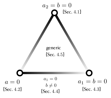
Figure 1: A summary of the classification in this section. The interior of the triangle represents the generic case where none of the parameters vanish, and the sides and vertices represent the various particular cases; recall $a_{1}\equiv{\rm Re}a$, $a_{2}\equiv{\rm Im}a$. The shading of the sides is meant to suggest which limits reproduce the cases represented by the vertices. For example, if one takes the equations for the $a_{1}=0$ case (lower side) and takes the $a_{2}\to 0$ limit, one recovers the equations of the $a=0$ case, while the same is not true if one takes the $b\to 0$ limit.

Strictly speaking one only needs to distinguish three cases.

• Generic case: $a_{1}\neq 0$ (section 4.5). In this case one needs to solve the PDEs (4.67) and (4.70). In the case with and without $F_{0}$, these reduce respectively to either (4.74) or (4.76). The solutions can be viewed as a certain decoration by extra fluxes of the particular case $a_{2}=b=0$ (upper vertex in figure 1, section 4.1), where $M_{6}=T^{2}\times S^{2}\times M_{2}$ and which can roughly be interpreted as systems of NS5s, D6s and D8s.

• $a_{1}=0$, $b\neq 0$ (section 4.4; lower side in figure 1). Here one needs to solve (4.60). There is in this class always an abelian isometry, T-dualizing along which produces a conformal Calabi–Yau-type solution [5, 6, 7, 8] (conformal Calabi–Yau’s with $(2,1)$ primitive flux). Again one can view the solutions as a decoration by extra fluxes of the particular case $a=0$ (lower-left vertex in figure 1, section 4.2), where $M_{6}=S^{1}\times S^{2}\times M_{3}$.

• $a_{1}=b=0$ (section 4.3). In this case the system is the rather more complicated (4.34)–(4.35), although we did manage to simplify it considerably and solve it with several Ansätze. Among these, we found some known D4–D6 systems, and some generalizations thereof. This case is in a sense the most interesting one.

We will see now some examples.

5 Examples

In section 4 we classified solutions to our minimal class, as defined in section 2. The classification was organized in several cases; in each of these the requirement of preserved supersymmetry was reduced to a system of PDEs. In this section, we will look at some particular solutions of these systems. In section 5.1 we will look at cases where $M_{6}$ is compact, namely at Minkowski compactifications. In later subsections we will do the exercise of applying the systems to AdS solutions. In particular, we will recover the AdS₇ and AdS₅ solutions of [21, 23] and [24], and we will write AdS₆ solutions in terms of a Toda-like equation which presumably reproduces the solutions in [37, 38]. For AdS₅, the only solutions in our class will actually be those of [24].

5.1 Compact $M_{6}$

We will now try to find examples where $M_{6}$ is compact, in some of the classes considered in 4. The classification there produced a vast array of possible systems, and our analysis here should be regarded as preliminary.

[$b=a_{2}=0$.]

Let us start from the $b=a_{2}=0$ case of section 4.1. Specifically, we will look at the $F_{0}=0$ case, as in section 4.1.1. We reduced there the problem to the single PDE (4.11). We collect the data of the solution here:

$$\begin{split}ds^{2}&=e^{2A}ds^{2}_{{\rm Mink}_{4}\times T^{2}}+\partial_{x_{1}}h\left(e^{2A}dx_{1}^{2}+e^{-2A}(dx_{2}^{2}+x_{2}^{2}ds^{2}(S^{2}))\right)\ ,\\ e^{2\Phi}&=e^{6A}\partial_{x_{1}}h\ ,\qquad B=x_{2}^{2}\partial_{x_{2}}h\text{Vol}(S^{2})\ ,\qquad F_{2}=c_{1}\text{Vol}(S^{2})\ .\end{split}$$ (5.1)

To find solutions, we can impose a separation of variables Ansatz $h=f(x_{1})g(x_{2})$. Then (4.11) imposes

$$\partial_{x_{1}}^{2}f+cf=0\ ,\qquad\partial^{2}_{x_{2}}(x_{2}g)=c(c_{1}+c_{2}x_{2})g,$$ (5.2)

which have closed form solutions. For $c=0$ we have compact solutions for $h=Cx_{1}\frac{a-x_{2}}{x_{2}}$, $e^{4A}=x_{2}/c_{1}$, if we take $x_{1}$ to be periodically identified with itself. So (5.1) becomes

$$\begin{split}ds^{2}&=\sqrt{\frac{x_{2}}{c_{1}}}ds^{2}_{{\rm Mink}_{4}\times T^{2}}+C\left(\frac{a}{x_{2}}-1\right)\left(\sqrt{\frac{x_{2}}{c_{1}}}dx_{1}^{2}+\sqrt{\frac{c_{1}}{x_{2}}}(dx_{2}^{2}+x_{2}^{2}ds^{2}(S^{2}))\right)\ ,\\ e^{2\Phi}&=\frac{C}{c_{1}^{3/2}}\sqrt{x_{2}}(a-x_{2})\ ,\qquad H=aCdx_{1}\wedge\text{Vol}(S^{2})\ ,\qquad F_{2}=c_{1}\text{Vol}(S^{2})\ .\end{split}$$ (5.3)

If the factor $\big{(}\frac{a}{x_{2}}-1\big{)}$ were $\left(1+\frac{a}{x_{2}}\right)$, this would represent a near-horizon D6 with an NS5 smeared along the $x_{1}$ direction. With $\left(1-\frac{a}{x_{2}}\right)$, the NS5 would be replaced by a more peculiar object, an ONS5-plane. As it is, (5.3) is a compact solution which behaves close to $x_{2}=0$ as a D6/NS5, and close to $x_{2}=a$ as a D6/ONS5, both NS objects being smeared along $x_{1}$. The solution is however highly curved everywhere: playing with the parameters (and taking flux quantization into account) one cannot make $a$ large. Solutions of this type, obtained by reversing signs in otherwise well-known solutions with orientifold planes, are easy to obtain, and we could exhibit several other such examples for other classes in section 4. We will not comment on such examples further. Notice however that the present example becomes much less trivial after one applies to it the solution-generating technique of section 4.5.

For $c>0$, (5.2) gives more interesting results. It can again be solved explicitly:

$$\begin{split}f&=-\cos(\sqrt{c}x_{1})\ ,\\ g&=e^{-\sqrt{cc_{2}}x_{2}}\left(\alpha{}_{1}F_{1}\left(1+\frac{c_{1}}{2}\sqrt{\frac{c}{c_{2}}},2,2\sqrt{cc_{2}}x_{2}\right)+\beta U\left(1+\frac{c_{1}}{2}\sqrt{\frac{c}{c_{2}}},2,2\sqrt{cc_{2}}x_{2}\right)\right)\end{split}$$ (5.4)

with $\alpha$ and $\beta$ two real parameters. For example, let us assume $c_{2}>1$, $c_{1}<0$, so that $e^{-4A}=c_{2}+\frac{c_{1}}{x_{2}}$ from (4.9) corresponds to an O6 at $x_{2}=x_{2}^{-}=-\frac{c_{1}}{c_{2}}$. Now $\partial_{x_{1}}h$ in (5.1) is $\sqrt{c}\sin(\sqrt{c}x_{1})g(x_{2})$. The fact that $\sin(\sqrt{c}x_{1})$ has a simple zero at $x_{1}=0,\frac{\pi}{\sqrt{c}}$ signals the presence at those loci of NS5s smeared along $x_{2}$ and the $S^{2}$. Moreover, by adjusting the $\beta/\alpha$, one can arrange for $g$ to have a simple zero at some finite value $x_{2}=x_{2}^{+}$. This signals the presence there of an ONS5. This time we then take $x_{1}\in[0,\frac{\pi}{\sqrt{c}}]$, $x_{2}\in[x_{2}^{-},x_{2}^{+}]$. Flux quantization fixes $c_{1}$ and $\alpha$. It appears to be possible to achieve weak curvature and weak coupling by adjusting the remaining parameters. The presence of so many sources, one of which a bit exotic, should make one cautious. But this is only one possible example of this type; clearly it is promising to explore such solutions further.

[$a=0$.]

As we have stressed earlier, this subclass is T-dual to the well-known conformal Calabi–Yau-type solutions in [5, 6, 7, 8] (conformal Calabi–Yau’s with $(2,1)$ primitive flux).

However, even in this class we find something interesting. Let us consider (4.2.1): as we observed there, the metric is formally of the D4-brane type. If we choose the particularly simple harmonic function $h=4(a-x_{2})$ and the constant $c=a\sin\theta_{0}$, with $a>0$, $\theta_{0}\in(0,\pi/2)$, the Minkowski warp factor in (4.2.1) is

$$e^{-4A}=\frac{(a_{+}-x_{2})(x_{2}-a_{-})}{x_{2}^{2}}\ ,\qquad a_{\pm}=\frac{a}{2}(1\pm\cos\theta_{0})\ .$$ (5.5)

The coordinate $x_{2}$ can be taken to belong in the range $(a_{-},a_{+})$; at both extrema, the metric’s behavior is that of an O4 smeared along directions $x_{1}$ and $x_{3}$. The fluxes read

$$\begin{split}H&=aL^{2}\sin\theta_{0}dx_{3}\wedge{\cal C}_{2}\ ,\qquad F_{2}=-\frac{aL^{2}}{c_{1}^{3/2}}\sin\theta_{0}{\cal C}_{2},\\ F_{4}&=\frac{4aL^{4}}{c_{1}^{3/2}}\left(1-\frac{a}{2x_{2}}\sin^{2}\theta_{0}\right)dx_{1}\wedge dx_{3}\wedge\text{Vol}(S^{2})\ .\end{split}$$ (5.6)

where ${\cal C}_{2}$ is defined in (4.2.1). As remarked earlier, if we T-dualize this example along $x_{4}$ we obtain a D3-type solution; technically, the internal space is a conformal Calabi–Yau. However, this solution should not be interpreted, as is usually done for such solutions, as the result of backreaction of O3-planes and D3-branes on a preexisting Calabi–Yau. The internal space $M_{6}$ looks rather like a $T^{3}\times S^{3}$ with two O3-planes at the two poles of the $S^{3}$, smeared along the $T^{3}$. The reason this falls in the conformal Calabi–Yau class is the accident that $S^{3}$ is itself conformally flat. If one is (rightly) not happy about the fact that the O3-planes are smeared, one can T-dualize instead along the directions $x_{1}$, $x_{3}$, to obtain a IIA solution again with $M_{6}=T^{3}\times S^{3}$, but with O6-planes extended along the $T^{3}$ and with two O6-planes at the poles of the $S^{3}$. Moreover, we have studied flux quantization and we have found no obstruction to making the solution weakly curved and weakly coupled (away from the two O6-planes), although we refrain from giving the results here.

5.2 AdS₇

We will now show how to recover the AdS₇ solutions of [21, 23] as particular examples of the system in section 4.1.2. As we explained there (see footnote 4), the relevant equation (4.13) is in fact the one derived in [26, 27]. A relation between those papers and the AdS₇ solutions was conjectured already in [21], but never realized until now.

We will use the customary trick of viewing AdS₇ solutions as Mink₆ solutions (mentioned in (2.5) for AdS₅). Thus in (4.5) we replace $T^{2}$ by $\mathbb{R}^{2}$, and we take $e^{A}=e^{\rho+A_{7}}$. We then try to rewrite the metric for the remaining four directions as

$$ds^{2}_{4}=e^{2A_{7}}d\rho^{2}+ds^{2}_{3}\ .$$ (5.7)

In order to do so, we define the following change of variables:

$$x_{1}=f(z)e^{2\rho},\qquad x_{2}=g(z)e^{4\rho}\ .$$ (5.8)

Imposing that (4.5) does indeed look like (5.7) gives two conditions: one from the $d\rho^{2}$ coefficient, one from setting to zero the coefficient of $d\rho dz$. This results in

$$\partial_{z}f=\frac{16g^{2}\partial_{z}(e^{-4A_{7}})}{8f-e^{4A_{7}}F_{0}}\ ,\qquad\partial_{z}g=-e^{4A_{7}}\frac{8fg\partial_{z}(e^{-4A_{7}})}{8f-e^{4A_{7}}F_{0}}\ .$$ (5.9)

With these definitions, it turns out that eq (4.13) is solved automatically. We can then use reparametrisation invariance to choose

$$g=e^{4A_{7}}\sqrt{\frac{1}{8}(\frac{3c_{1}F_{0}^{2}}{16}-F_{0}f)}\ ,$$ (5.10)

which reduces (5.9) to a single ODE:

$$\partial_{z}(e^{4A_{7}})=\frac{8\partial_{z}f(F_{0}e^{4A_{7}}-8f)}{F_{0}(3c_{1}F_{0}-16f)}\ .$$ (5.11)

This is solved by

$$e^{4A_{7}}=c_{1}+\frac{8f}{3F_{0}}+\frac{4\tilde{c}_{2}}{F_{0}\sqrt{16f-3c_{1}F_{0}}}\ .$$ (5.12)

where $\tilde{c}_{2}$ is an integration constant. Since $e^{4A_{7}}$ is actually just a function of $f$, we can choose $f$ such that expressions simplify. Taking

$$f=\frac{3F_{0}}{8}\left(\frac{c_{1}}{2}+z^{2}\right),$$ (5.13)

and redefining $\tilde{c}_{2}$ in terms of a new constant $c_{2}$ we get

$$e^{4A_{7}}=\frac{2z^{3}+3c_{1}z+2c_{2}}{2z}\ ,$$ (5.14)

which is proportional to $\frac{\alpha}{\ddot{\alpha}}$, for $\alpha$ a cubic function. This is the expression for $e^{4A_{7}}$ one can find in [41, Eq. (2.27)]; $\alpha=\sqrt{\beta}$ can be found in (2.26) there and is indeed a cubic function. So our $z$ here is linearly related to the $z$ there. One can also check that the local expression for the dilaton, metric and fluxes that we obtain from section 4.1.2 reproduce those in [41, Eq. (2.27)–(2.29)].

5.3 AdS₆

We will now use a similar logic to the problem of AdS₆ solutions in IIB using section 4.3. These have been treated in [30], where the problem was reduced to two hard PDEs for the warping and dilaton (which were later confirmed in [44]). Recently, the general solution was found in [37, 38] by reanalyzing the problem in a clever coordinate system.

Since we are actually interested in IIB solutions, our Ansatz will correspond to a formal T-dual of such a solution along one of the spacetime directions:

$$ds^{2}=4e^{2A_{6}}\bigg{(}e^{2\rho}dx^{2}_{1,3}+d\rho^{2}\bigg{)}+\frac{1}{4}e^{-2\rho-2A_{6}}dx_{4}^{2}+ds^{2}(M_{4}),~{}~{}~{}e^{\Phi}=e^{\Phi_{\rm IIB}-\rho-A_{6}}\ ;$$ (5.15)

Thus in particular $e^{2A}=4e^{2A_{6}+2\rho}$, where the 4 is inserted for convenience as it simplifies later expressions. $M_{4}$ is spanned by $S^{2}$ and two other coordinates. $x_{4}$ is the direction along which T-duality will produce an AdS₆ solution in IIB. The fluxes can be found in (4.33) from which one sees that while $\partial_{x_{4}}$ is not an isometry in general, it is possible to impose that it is. We will try to rewrite the metric of section 4.3 in this form so that it reduces to (5.15). Similarly to (5.8), we will change coordinates:

$$x_{1}=e^{-3\rho}f(r,y)\ ,\qquad x_{2}=\frac{4}{9}e^{3\rho}y\ ,\qquad x_{3}=4re^{\rho-\frac{1}{3}\Delta(r,y)}\ .$$ (5.16)

We correspondingly write $e^{2C}H_{1}=d(e^{2C}B_{0})$ (recall (3.5b)) as

$$e^{2C}H_{1}=h_{1}(r,y)dr+h_{2}(r,y)dy\ ,$$ (5.17)

Imposing that the metric has no $d\rho$ cross terms and that the coefficient of $d\rho^{2}$ is correct leads to

$$\begin{split}e^{\Phi_{\rm IIB}}&=6\frac{e^{-\frac{2}{3}\Delta+4\lambda}+e^{12\lambda}f^{2}}{e^{8\lambda}-y^{2}},\\ h_{1}&=\frac{4y}{9f}\bigg{(}r(3-r\partial_{r}\Delta)e^{-\frac{2}{3}\Delta-8\lambda}-f\partial_{r}f\bigg{)}\ ,\qquad h_{2}=\frac{4y}{9}(f\partial_{y}\Delta-\partial_{y}f)\ ,\end{split}$$ (5.18)

where to simplify things we have made the choice

$$e^{4A_{6}}=\frac{1}{6}e^{4\lambda+\Phi_{\rm IIB}}\ .$$ (5.19)

Diffeomorphism invariance now gives us the freedom to choose $\Delta$ such that the metric also has no $drdy$ cross term, which actually defines the warp factor in terms of $\Delta$ as

$$e^{-8\lambda}=\frac{\partial_{y}\Delta}{y(1+y\partial_{y}\Delta)}.$$ (5.20)

This leaves us with two functions, $f$ and $\Delta$ which the physical fields are defined in terms of, but we are yet to impose the supersymmetry constraints (4.28c), these lead to

$$f=-e^{\frac{1}{3}\Delta}\frac{3-r\partial_{r}\Delta}{(1+y\partial_{y}\Delta)}\ ,\qquad\partial^{2}_{r}(e^{\frac{1}{3}\Delta})=\frac{1}{3}\partial_{y}^{2}e^{-\Delta}\ ,$$ (5.21)

from which it follows that the NS 3-form is closed and that the Bianchi identities of the RR sector are all satisfied. The second condition is reminiscent of (but not the same as) a Toda equation, such as the one we will review in section 5.4. It is much simpler than the PDEs in [30] ; it should be solved by the metrics in [37, 38]. T-dualizing to IIB, the metric reads

$$ds^{2}=4e^{2A_{6}}\bigg{(}ds^{2}_{\rm AdS_{6}}+\frac{y\partial_{y}\Delta}{9(1+y\partial_{y}\Delta)}ds^{2}(S^{2})+\frac{\partial_{y}\Delta}{9y}\big{(}dy^{2}+e^{-\frac{4}{3}\Delta}dr^{2}\big{)}\bigg{)}\,$$ (5.22)

while the fluxes on the other hand

$$F_{1} =\bigg{(}\frac{27}{4y^{2}}e^{-2/3\Delta+8\lambda-2\Phi}fh_{2}-\frac{2}{3}e^{-2/3\Delta-\lambda-7/4\Phi}\partial_{y}(ye^{-3\lambda+3/4\Phi})\bigg{)}dr$$

$$-\bigg{(}\frac{27}{4y^{2}}e^{2/3\Delta+8\lambda-2\Phi}fh_{2}-\frac{2}{3}e^{2/3\Delta-\lambda-7/4\Phi}\partial_{r}(ye^{-3\lambda+3/4\Phi})\bigg{)}dy,$$ (5.23)

$$F_{3} =\frac{y}{54}e^{-2/3\Delta-4\lambda-\Phi}\bigg{(}(45h_{2}+32y\partial_{y}f+96yf\partial_{y}\lambda)dr+(45h_{1}+32y\partial_{r}f+96yf\partial_{r}\lambda)e^{4/3\Delta}dy\bigg{)}\wedge\text{Vol}(S^{2}).$$

A particularly simple solution is given by

$$e^{\Delta}=\frac{c_{1}r^{3}}{c_{2}-y},$$ (5.24)

which gives rise to the Hopf fibre T-dual of the unique $AdS_{6}$ solution in IIA. As there is no uniqueness theorem in IIB, and indeed examples beyond the IIA T-dual are already known, our hope is that this formulation will prove useful to further populate the class of such solutions. We leave this however for future work.

5.4 AdS₅

We will now also show how to recover in IIA the AdS₅ solutions obtained in M-theory by [24] from section 4.3.

The strategy is similar as the one we used in the previous subsections, and we will be brief. Once again we use the trick (2.5); however, we actually define $e^{2A}=4e^{2\rho+2A_{5}}$, to match the conventions in [24]. These solutions have an enhanced SU(2)$\times$ U(1) R-symmetry which should be manifest in the geometry in appropriate coordinates. If we impose rotational symmetry in $(x_{3},x_{4})$ we introduce a U(1) isometry in the metric under which the pure spinors are charged, so this is the U(1) R-symmetry. This motivates the change of coordinates

$$x_{1}=f(r,y)e^{-2\rho}\ ,\qquad x_{2}=4ye^{2\rho}\ ,\qquad x_{3}+ix_{4}=4re^{\frac{1}{2}D(r,y)}e^{i\psi}e^{\rho},$$ (5.25)

where $\partial_{\psi}$ is part of the R-symmetry and the factors of $\rho$ are chosen such that the internal manifold has no $\rho$-dependent warping. We then express

$$e^{2C}H_{1}=h_{1}(r,y)dr+h_{2}(r,y)dy,$$ (5.26)

which is the most general form consistent with the isometries. To obtain $AdS_{5}$ solutions, we also need to again impose that the cross-terms involving $d\rho$ vanish, and that the coefficient of $d\rho^{2}$ is correct. By imposing these conditions and that the metric is diagonal in all coordinates we fix the physical fields as

$$e^{2A_{5}} =e^{2\lambda+2/3\Phi}\ ,\qquad e^{-6\lambda}=\frac{-\partial_{y}D}{y(1-y\partial_{y}D)}\ ,\qquad e^{4/3\Phi-2\lambda}=\frac{r^{2}e^{D}+16f^{2}e^{6\lambda}}{e^{6\lambda}-y^{2}},$$ (5.27)

$$h_{1} =rye^{D-6\lambda}\frac{2+r\partial_{r}D}{4f}-4y\partial_{r}f\ ,\qquad h_{2}=\frac{y}{4f}\left(e^{-8\lambda+4/3\Phi}y+e^{D-6\lambda}r^{2}\partial_{y}D-16f\partial_{y}f\right)\ ,$$ (5.28)

where the first of these just defines $A_{5}$ in terms of an arbitrary function $\lambda(r,y)$. We now have two undefined functions $f$ and $D$, but we are yet to impose the conditions (4.28c); these lead to

$$f=\frac{2+r\partial_{r}D}{4(1-y\partial_{y}D)}\ ,\qquad\frac{1}{r}\partial_{r}(r\partial_{r}D)+\partial_{y}^{2}e^{D}=0\ .$$ (5.29)

up to the subtlety discussed in footnote 10. Thus, $D$ must obey the axially symmetric 3d Toda equation, and $f$ is fixed in terms of $D$. With these conditions the NS three-form is closed, and the fluxes obey the Bianchi identities. The solutions are then of the form

$$ds^{2} =e^{2\lambda+\frac{2}{3}\Phi}\bigg{(}4ds^{2}(AdS_{5})+\frac{-y\partial_{y}D}{1-y\partial_{y}D}ds^{2}(S^{2})+\frac{-\partial_{y}D}{y}(dy^{2}+e^{D}dr^{2})\bigg{)}+4e^{-2\lambda-\frac{2}{3}\Phi+D}r^{2}d\psi^{2},$$

$$C_{1} =-\frac{2y(2+r\partial_{r}D)}{\partial_{y}D}e^{-4\lambda-\frac{4}{3}\Phi}d\psi,~{}~{}~{}C_{3}=2y^{3}e^{-6\lambda}d\psi\wedge\text{Vol}(S^{2}),$$

$$H =\left(d\left[e^{-6\lambda}\frac{y^{2}}{\partial_{y}D}(2y\partial_{y}D+r\partial_{r}D)\right]-\partial_{y}(e^{D})rdr+r\partial_{r}Ddy\right)\wedge\text{Vol}(S^{2})$$ (5.30)

where $F_{2}=dC_{1}$ and $F_{4}=dC_{3}-H\wedge C_{1}$. The alert reader might notice that this solution does not actually correspond to imposing rotational symmetry in the $(x_{1},x_{2})$ plane of [45, Eq. (3.3)] then reducing to IIA along the isometry one has imposed on the solution. The reason for this, as we show in appendix D, is that reducing on this isometry breaks supersymmetry. The resolution is to perform the reduction on a linear combination of the two U(1)’s at ones disposal in the axially symmetric AdS₅ M-theory solutions which results in (5.4).

We thus have reproduced the solutions of [24], without any loss of generality. Thus, these solutions are the only one in massive IIA within our “minimal” class of manifolds. (This conclusion is similar to [46] in IIB.) If $\mathcal{N}=2$ $AdS_{5}$ solutions with non-zero Romans mass do exist, R-symmetry must act in a more complicated way, such as with a squashed $S^{3}$ as discussed in section 2.

Appendix A Spinors on $S^{2}$

To begin let us consider an arbitrary 2d Euclidean space. In general one can define the chiral spinors

$$\xi_{\pm}\ ,\qquad\xi^{c}_{\pm}=(\xi_{\pm})^{c}=B_{2}\xi_{\pm}^{*}=(\xi^{c})_{\mp}\ .$$ (A.1)

Let us work with the following basis of gamma matrices:

$$\gamma_{1}=\sigma_{1}\ ,\qquad\gamma_{2}=\sigma_{2}\ ,\qquad\hat{\gamma}=-i\gamma_{1}\gamma_{2}=\sigma_{3}\ ,\qquad B_{2}=\sigma_{2}\ ,\qquad B^{-1}_{2}\gamma_{\mu}B_{2}=-\gamma_{\mu}^{*}.$$ (A.2)

In terms of the spinors we can then define the following scalars:

$$|\xi_{\pm}|^{2}=\alpha^{2}_{\pm}\ ,\qquad\bar{\xi}_{-}\xi_{+}=-(\xi^{{\dagger}}_{-}\xi^{c}_{+})^{*}=-\bar{\xi}_{+}\xi_{-}=(\xi^{{\dagger}}_{+}\xi^{c}_{-})^{*}=\beta,$$ (A.3)

where $\alpha_{\pm}$ are real and $\beta$ is complex and as elsewhere $\overline{\xi}=(\xi^{c})^{{\dagger}}$. In general the scalars and spinors satisfy

$$\beta^{*}\xi_{\pm}=\pm\alpha^{2}_{\pm}\xi^{c}_{\mp}\ ,\qquad\beta\xi^{c}_{\pm}=\mp\alpha^{2}_{\pm}\xi_{\mp},$$ (A.4)

We define the vectors

$$v_{\pm}^{\mu}=\frac{1}{2}\xi_{\mp}^{{\dagger}}\gamma^{\mu}\xi_{\pm}\ ,\qquad u_{\pm}^{\mu}=\frac{1}{2}\overline{\xi}_{\pm}\gamma^{\mu}\xi_{\pm}\ ,\qquad\overline{u}_{\pm}^{\mu}=\frac{1}{2}\xi^{{\dagger}}_{\pm}\gamma^{\mu}\xi^{c}_{\pm},$$ (A.5)

We then have the following bispinor identities:

$$\begin{split}\xi_{\pm}\otimes\xi^{{\dagger}}_{\mp}&=-\xi^{c}_{\mp}\otimes\overline{\xi}_{\pm}=v_{\pm},\\ \xi_{\pm}\otimes\overline{\xi}_{\pm}&=u_{\pm}\ ,\qquad\xi^{c}_{\pm}\otimes\xi^{{\dagger}}_{\pm}=\overline{u}_{\pm},\\ \xi_{\pm}\otimes\xi^{{\dagger}}_{\pm}&=\left(\xi^{c}_{\pm}\otimes\overline{\xi}_{\pm}\right)^{*}=\frac{1}{2}\alpha_{\pm}^{2}(1\pm\hat{\gamma}),\\ \xi_{\pm}\otimes\overline{\xi}_{\mp}&=-\left(\xi^{c}_{\pm}\otimes\xi^{{\dagger}}_{\mp}\right)^{*}=\pm\frac{1}{2}\beta(1\pm\hat{\gamma}).\end{split}$$ (A.6)

Using these we find that the vectors act on the spinors as

$$v_{\pm}\xi_{\mp}=\alpha^{2}_{\mp}\xi_{\pm}\ ,\qquad v_{\pm}\xi^{c}_{\pm}=\mp\beta^{*}\xi_{\pm},$$

$$u_{\pm}\xi_{\mp}=\mp\beta\xi_{\pm}\ ,\qquad\overline{u}_{\pm}\xi_{\pm}=\alpha_{\pm}^{2}\xi^{c}_{\pm}\ ,\qquad u_{\pm}\xi^{c}_{\pm}=\alpha^{2}_{\pm}\xi_{\pm}\ ,\qquad\overline{u}_{\pm}\xi^{c}_{\mp}=\pm\beta^{*}\xi^{c}_{\pm},$$ (A.7)

with all else giving zero. It is then rather simple to show that

$$v_{+}.v_{-}=\frac{1}{2}\alpha^{2}_{+}\alpha^{2}_{-}\ ,\qquad u_{\pm}.\overline{u}_{\pm}=\frac{1}{2}\alpha_{\pm}^{4}\ .$$ (A.8)

This tells us that $v_{+}$ defines a complex vector whose conjugate is $v_{-}$, and $u_{\pm}$ define two complex vectors whose conjugates are $\overline{u}_{\pm}$. For completeness we quote the remaining non vanishing inner products of the vectors:

$$u_{\pm}.v_{\mp}=\mp\frac{1}{2}\beta\alpha_{\pm}^{2}\ ,\qquad\overline{u}_{\pm}.v_{\pm}=\mp\frac{1}{2}\beta^{*}\alpha_{\pm}^{2}\ ,\qquad u_{\pm}.u_{\mp}=-\frac{1}{2}\beta^{2}\ ,\qquad\overline{u}_{\pm}.\overline{u}_{\mp}=-\frac{1}{2}(\beta^{*})^{2},$$ (A.9)

although they are not used in the main text. We will however need certain Lie brackets. For instance one can show that

$$[u_{\pm},\overline{u}_{\mp}]=\frac{1}{2}\gamma_{\mu\nu}\bigg{(}-4v^{\mu}_{\pm}v^{\nu}_{\pm}+\overline{\xi}_{\pm}\gamma^{\mu\nu}v_{\pm}\xi^{c}_{\mp}\bigg{)}=0\ .$$ (A.10)

The full list of non vanishing Lie brackets is

$$\begin{split}&[u_{\pm},\overline{u}_{\pm}]=\pm\alpha^{4}_{\pm}\hat{\gamma}\ ,\qquad~{}[u_{\pm},u_{\mp}]=\pm\beta^{2}\hat{\gamma},\\ &[v_{\pm},u_{\mp}]=\alpha^{2}_{\mp}\beta\hat{\gamma}\ ,\qquad[v_{\pm},\overline{u}_{\pm}]=-\alpha^{2}_{\pm}\beta^{*}\hat{\gamma}\ .\end{split}$$ (A.11)

On $S^{2}$, there exist in particular Killing spinors, namely $\xi_{\pm}$ which satisfy

$$\nabla_{\mu}\xi_{\pm}=\frac{i}{2}\gamma_{\mu}\xi_{\mp}\ ,\qquad\nabla_{\mu}\xi^{c}_{\pm}=\frac{i}{2}\gamma_{\mu}\xi^{c}_{\mp}\ .$$ (A.12)

From these it follows that

$$\nabla(\xi^{{\dagger}}_{\pm}\xi_{\pm})=\nabla(\overline{\xi}_{\pm}\xi^{c}_{\pm})=\mp i(v_{+}-v_{-})\ ,\qquad\nabla(\overline{\xi}_{\mp}\xi_{\pm})=\mp i(u_{+}-u_{-})\ ,\qquad\nabla(\xi^{{\dagger}}_{\mp}\xi^{c}_{\pm})=\mp i(\overline{u}_{+}-\overline{u}_{-}),$$ (A.13)

which tell us that none of the scalar bilinears in (A.3) are constant. However certain combinations are: for instance we have $\nabla(\alpha_{+}^{2}+\alpha_{-}^{2})=0$, which we can use to set

$$\alpha_{+}^{2}+\alpha_{-}^{2}=1$$ (A.14)

without loss of generality.

We know that $S^{2}$ has a global SU(2) isometry; thus we should be able to define three Killing vectors $K^{a}$ whose Lie brackets realize the SU(2) Lie algebra:

$$[K^{a},K^{b}]=\epsilon^{abc}K^{c}\ .$$ (A.15)

This means that they should obey

$$\nabla_{\mu}K^{a}_{\nu}=\epsilon_{abc}K^{b}_{\mu}K^{c}_{\nu}\ .$$ (A.16)

These Killing vectors can be found in terms of spinor bilinears as

$$(K^{1})^{\mu}=(u^{\mu}_{+}+u^{\mu}_{-}+\overline{u}^{\mu}_{+}+\overline{u}^{\mu}_{-}),$$

$$(K^{2})^{\mu}=-i(u^{\mu}_{+}+u^{\mu}_{-}-(\overline{u}^{\mu}_{+}+\overline{u}^{\mu}_{-})),$$ (A.17)

$$(K^{3})^{\mu}=2(v^{\mu}_{+}+v^{\mu}_{-}).$$

To see that these indeed satisfy (A.16), we can compute their covariant derivatives using (A.5):

$$\nabla_{\mu}(K^{1}+iK^{2})_{\nu} =-i(\overline{\xi}_{+}\gamma_{\mu\nu}\xi_{-}+\overline{\xi}_{-}\gamma_{\mu\nu}\xi_{+})=2\beta\epsilon_{\mu\nu},$$

$$\nabla_{\mu}(K^{1}-iK^{2})_{\nu} =-i(\xi^{{\dagger}}_{+}\gamma_{\mu\nu}\xi^{c}_{-}+\xi^{{\dagger}}_{-}\gamma_{\mu\nu}\xi^{c}_{+})=2\beta^{*}\epsilon_{\mu\nu},$$

$$\nabla_{\mu}(K^{3})_{\nu} =-i(\xi^{{\dagger}}_{+}\gamma_{\mu\nu}\xi_{+}+\xi^{{\dagger}}_{-}\gamma_{\mu\nu}\xi_{-})=(\alpha_{+}^{2}-\alpha_{-}^{2})\epsilon_{\mu\nu}\ .$$ (A.18)

These are all antisymmetric; so indeed $\nabla_{(\mu}K^{a}_{\nu)}=0$, and so the $K^{a}$ are Killing vectors. To show they obey the SU(2) relations, we can use the Lie bracket in (A.10) and that

$$\frac{1}{2}\epsilon_{abc}[K^{b},K^{c}]=\epsilon_{abc}K^{b}_{\mu}K^{c}_{\nu}\gamma^{\mu\nu}\ ,\qquad~{}\hat{\gamma}=-\frac{i}{2}\epsilon_{\mu\nu}\gamma^{\mu\nu}\ .$$ (A.19)

For example

$$\epsilon_{3bc}K^{b}_{\mu}K^{c}_{\nu}\gamma^{\mu\nu}=[K^{1},K^{2}]=2i([u_{+},\overline{u}_{+}]+[u_{-},\overline{u}_{-}])=(\alpha^{2}_{+}+\alpha^{2}_{-})(\alpha^{2}_{+}-\alpha^{2}_{-})\epsilon_{\mu\nu}\gamma^{\mu\nu}\ ,$$ (A.20)

which given (A.14) is equal to $\nabla_{\mu}(K_{3})_{\nu}\gamma^{\mu\nu}$. One can check the other SU(2) relations in a similar fashion.

Having established that $K^{a}$ are the SU(2) Killing vectors, we choose to parameterise them as

$$K^{a}=\epsilon_{abc}y_{b}dy_{c}\ ,\qquad\ ,$$ (A.21)

in terms of the “embedding coordinates” $y^{a}$ for the $S^{2}$, which obey

$$y_{1}^{2}+y_{2}^{2}+y_{3}^{2}=1\ .$$ (A.22)

Consistency of the SU(2) algebra relation with (A) then implies that

$$\alpha^{2}_{\pm}=\frac{1}{2}(1\pm y_{3})\ ,\qquad\beta=\frac{1}{2}(y_{1}+iy_{2})\ .$$ (A.23)

The spinorial Lie derivative along one of these Killing vectors is given by

$$\mathcal{L}_{K^{a}}\xi_{\pm} =(K^{a})^{\mu}\nabla_{\mu}\xi_{\pm}+\frac{1}{4}\nabla_{\mu}K^{a}_{\nu}\gamma^{\mu\nu}\xi_{\pm},$$

$$=\frac{i}{2}\bigg{(}K^{a}\xi_{\mp}-\frac{i}{2}(\nabla K^{a})\xi_{\pm}\bigg{)}$$ (A.24)

and similarly for $\xi^{c}_{\pm}$. Using (A) and (A) one finds

$$K^{1}\xi_{\pm}=\mp\beta\xi_{\mp}-\alpha^{2}_{\pm}\xi^{c}_{\pm}\ ,\qquad K^{1}\xi^{c}_{\pm}=\alpha^{2}_{\pm}\xi_{\pm}\mp\beta^{*}\xi^{c}_{\mp}\ ,\qquad(\nabla K^{1})=2i(\beta+\beta^{*})\hat{\gamma}$$

$$K^{2}\xi_{\pm}=-i(\pm\beta\xi_{\mp}-\alpha^{2}_{\pm}\xi^{c}_{\pm})\ ,\qquad K^{2}\xi^{c}_{\pm}=i(\alpha^{2}_{\pm}\xi_{\pm}\mp\beta^{*}\xi^{c}_{\mp})\ ,\qquad(\nabla K^{2})=2(\beta-\beta^{*})\hat{\gamma}$$

$$K^{3}\xi_{\pm}=2\alpha^{2}_{\pm}\xi_{\mp}\ ,\qquad K^{3}\xi^{c}_{\pm}=-2\alpha^{2}_{\pm}\xi^{c}_{\mp}\ ,\qquad\qquad(\nabla K^{3})=2i(\alpha^{2}_{+}-\alpha^{2}_{-})\hat{\gamma},$$ (A.25)

which is sufficient to show that

$$\vec{\xi}_{\pm}=\left(\begin{array}[]{l}\xi_{\pm}\\ \xi^{c}_{\mp}\end{array}\right)$$ (A.26)

transforms as a doublet. For instance,

$$K^{3}\vec{\xi}_{\mp}-\frac{i}{2}(\nabla K^{3})\vec{\xi}_{\pm}=\left(\begin{array}[]{cc}2\alpha^{2}_{\mp}\mp(\alpha_{\pm}^{2}-\alpha_{\mp}^{2})\hat{\gamma}&0\\ 0&-2\alpha^{2}_{\pm}\mp(\alpha_{\pm}^{2}-\alpha_{\mp}^{2})\hat{\gamma}\end{array}\right)\left(\begin{array}[]{c}\xi_{\pm}\\ \xi^{c}_{\mp}\end{array}\right)=\sigma_{3}\vec{\xi}_{\pm}.$$ (A.27)

Performing similar calculations for $K^{1,2}$ one can show that in general

$$\mathcal{L}_{K^{a}}\vec{\xi}=\frac{i}{2}\sigma_{a}\vec{\xi}\ .$$ (A.28)

Actually (A.26) is not the most general doublet: we can add a phase to each component without changing the transformation properties. In fact the most general doublet we can write is

$$\vec{\xi}_{\pm}=\left(\begin{array}[]{l}\xi_{\pm}\\ e^{i\delta}\xi^{c}_{\mp}\end{array}\right)\ .$$ (A.29)

A possible phase in the first entry can be absorbed into the definition of $\xi_{\pm}$.

Appendix B Pure spinors from six to four dimensions

In terms of the vectors introduced in appendix A, one can parametrize the bispinors on $S^{2}$ as

$$\xi_{\pm}\otimes\xi^{{\dagger}}_{\pm}=\frac{1}{4}(1\pm y_{3})(1\mp ie^{2C}\text{Vol}(S^{2}))\ ,\qquad\xi_{\pm}\otimes\xi^{{\dagger}}_{\mp}=\frac{1}{4}e^{C}(K_{3}\pm idy_{3}),$$

$$\xi_{\pm}\otimes\overline{\xi}_{\pm}=\frac{1}{4}e^{C}(K_{z}\pm idz)\ ,\qquad\xi_{\pm}\otimes\overline{\xi}_{\mp}=\pm\frac{1}{4}z(1\mp ie^{2C}\text{Vol}(S^{2})),$$ (B.1)

where we define $z=y_{1}+iy_{2}$, $K_{z}=K_{1}+iK_{2}$ to ease presentation. This means the 6d bispinors implied by (3.1) are

$$\Phi_{-} =\frac{1}{4}\bigg{[}\Psi^{1}_{+}-\Psi^{1}_{-}+y_{3}(\Psi^{1}_{+}+\Psi^{1}_{-})+e^{C}K_{3}\wedge(\Psi^{2}_{+}+\Psi^{2}_{-})$$ (B.2)

$$+i\bigg{(}e^{C}dy_{3}\wedge(\Psi^{2}_{+}-\Psi^{2}_{-})-e^{2C}\text{Vol}(S^{2})\wedge(\Psi^{1}_{+}+\Psi^{1}_{-})-e^{2C}y_{3}\text{Vol}(S^{2})\wedge(\Psi^{1}_{+}-\Psi^{1}_{-})\bigg{)}\bigg{]},$$

$$\Phi_{+} =\frac{1}{4}\bigg{[}z(\tilde{\Psi}^{2}_{+}-\tilde{\Psi}^{2}_{-})-e^{C}K_{z}\wedge(\tilde{\Psi}^{1}_{+}-\tilde{\Psi}^{1}_{-})-i\bigg{(}e^{C}dz\wedge(\tilde{\Psi}^{1}_{+}+\tilde{\Psi}^{1}_{-})+ze^{2C}\text{Vol}(S^{2})\wedge(\tilde{\Psi}^{2}_{+}+\tilde{\Psi}^{2}_{-})\bigg{)}\bigg{]}.$$

Here

$$\Psi^{1}_{\pm}=\eta^{1}_{\pm}\otimes\eta^{2{\dagger}}_{\mp}\ ,\qquad~{}\Psi^{2}_{\pm}=\eta^{1}_{\pm}\otimes\eta^{2{\dagger}}_{\pm},$$

$$\tilde{\Psi}^{1}_{\pm}=\eta^{1}_{\pm}\otimes\overline{\eta}^{2}_{\mp}\ ,\qquad~{}\tilde{\Psi}^{2}_{\pm}=\eta^{1}_{\pm}\otimes\overline{\eta}^{2}_{\pm}.$$ (B.3)

These are in fact the even and odd parts of (3.4).

Plugging (B.2) in the supersymmetry conditions (3.3) gives 8 independent conditions on $M_{4}$. To express these we decompose the NSNS three-form as

$$H=H_{3}+e^{2C}H_{1}\wedge\text{Vol}(S^{2})\ ,\qquad H=dB\ ,\qquad B=B_{2}+e^{2C}B_{0}\text{Vol}(S^{2}).$$ (B.4)

We obtain two equations from (3.3a):

$$d_{H_{3}}\big{(}e^{3A+C-\Phi}\tilde{\Psi}^{\text{odd}}\big{)} =ie^{3A-\Phi}\tilde{\Psi}_{\hat{\gamma}}^{\text{even}},$$ (B.5a)

$$d_{H_{3}}\big{(}e^{3A+2C-\Phi}\tilde{\Psi}^{\text{even}}\big{)} =ie^{3A+2C-\Phi}H_{1}\wedge\tilde{\Psi}_{\hat{\gamma}}^{\text{even}}+2ie^{3A+C-\Phi}\tilde{\Psi}_{\hat{\gamma}}^{\text{odd}};$$ (B.5b)

four from (3.3b):

$$d_{H_{3}}\big{(}e^{2A-\Phi}\text{Re}\Psi_{\hat{\gamma}}^{\text{odd}}\big{)} =0,$$ (B.6a)

$$d_{H_{3}}\big{(}e^{2A+C-\Phi}\text{Re}\Psi_{\hat{\gamma}}^{\text{even}}\big{)} =e^{2A-\Phi}\text{Re}\Psi^{\text{odd}},$$ (B.6b)

$$d_{H_{3}}\big{(}e^{2A+2C-\Phi}\text{Im}\Psi^{\text{odd}}\big{)} =e^{2A+2C-\Phi}H_{1}\wedge\text{Re}\Psi_{\hat{\gamma}}^{\text{odd}},$$ (B.6c)

$$d_{H_{3}}\big{(}e^{2A+2C-\Phi}\text{Im}\Psi_{\hat{\gamma}}^{\text{odd}}\big{)} =e^{2A+2C-\Phi}H_{1}\wedge\text{Re}\Psi^{\text{odd}}+2e^{2A+C-\Phi}\text{Re}\Psi^{\text{even}}\ ;$$ (B.6d)

and finally, two from (3.3c):

$$d_{H_{3}}\big{(}e^{4A+C-\Phi}\text{Re}\Psi^{\text{even}}\big{)} =e^{4A-\Phi}\text{Im}\Psi^{\text{odd}},$$ (B.7a)

$$d_{H_{3}}\big{(}e^{4A+2C-\Phi}\text{Re}\Psi_{\hat{\gamma}}^{\text{odd}}\big{)} =e^{4A+2C-\Phi}H_{1}\wedge\text{Im}\Psi^{\text{odd}}-2e^{4A+C-\Phi}\text{Im}\Psi^{\text{even}}\ .,$$ (B.7b)

The remaining conditions imply the fluxes. To express these we decompose the internal part of RR polyforms as

$$f=F+e^{2C}\text{Vol}(S^{2})\wedge G,$$ (B.8)

which leads to the flux conditions

$$d_{H_{3}}\big{(}e^{4A-\Phi}\text{Im}\Psi_{\hat{\gamma}}^{\text{odd}}\big{)} =\frac{1}{2}e^{4A}\star_{4}\lambda(G),$$ (B.9a)

$$d_{H_{3}}\big{(}e^{4A+2C-\Phi}\text{Re}\Psi^{\text{odd}}\big{)} =-e^{4A+2C-\Phi}H_{1}\wedge\text{Im}\Psi_{\hat{\gamma}}^{\text{odd}}-\frac{1}{2}e^{4A+2C}\star_{4}\lambda(F).$$ (B.9b)

These conditions are rather restrictive: for example, it is already clear that the zero form parts of $\Psi$ and $\tilde{\Psi}_{\hat{\gamma}}$ must vanish, (3.6).

Appendix C Alternative classification of $b=a_{1}=0$ case

In this appendix we give an alternative classification to section 4.3, in term of $B_{0}$ rather than $H_{1}=e^{-2C}d(e^{2C}B_{0})$. Upon setting $b=a_{1}=0,~{}a_{2}=1$ one can show that the supersymmetry conditions of appendix B all follow from

$$B_{2}=0,$$ (C.1a)

$$d(e^{A}w)=0,~{}~{}~{}d(e^{2A+C-\Phi})+e^{2A-\Phi}v_{2}=0,~{}~{}~{}d(e^{-2A+\Phi}(v_{1}+B_{0}v_{2}))=0,$$ (C.1b)

$$d(e^{-\Phi}v_{1})\wedge w\wedge\overline{w}=0,~{}~{}~{}d(e^{2C-\Phi}(B_{0}v_{1}-v_{2}))\wedge w\wedge\overline{w}=0,$$ (C.1c)

One can solve the conditions (C.1b) locally by defining the vielbein in terms of local coordinates $(x_{1},...,x_{4})$ as

$$v_{1}=e^{2A-\Phi}dx_{1}+B_{0}e^{-2A+\Phi}dx_{2},\qquad v_{2}=-e^{-2A+\Phi}dx_{2},\qquad w=e^{-A}(dx_{3}+idx_{4}),\qquad x_{2}=e^{2A+B-\Phi},$$

it then follows that (C.1c) imposes the PDEs

$$\partial_{x_{2}}\left(e^{2A-2\Phi}\right)=\partial_{x_{1}}\left(e^{-2A}B_{0}\right),$$

$$\partial_{x_{2}}\left(x_{2}^{2}e^{-2A}B_{0}\right)=\partial_{x_{1}}\left(x_{2}^{2}e^{-6A+2\Phi}(1+B_{0}^{2})\right),$$ (C.2)

but place no restriction on the various functions dependence on $(x_{3},x_{4})$, so we only have an a prior $\mathbb{R}_{1,3}$ factor in these solutions. Following the same prescription as the main text on can establish that the fluxes are given by

$$B= x_{2}^{2}e^{-4A+2\Phi}B_{0}\text{Vol}(S^{2}),$$

$$F_{2}= \big{(}\partial_{x_{4}}(e^{2A-2\Phi})dx_{3}-\partial_{x_{3}}(e^{2A-2\Phi})dx_{4}\big{)}\wedge dx_{1}+\big{(}\partial_{x_{4}}(e^{-2A}B_{0})dx_{3}-\partial_{x_{3}}(e^{-2A}B_{0})dx_{4}\big{)}\wedge dx_{2}$$

$$-\partial_{x_{1}}(e^{-4A})dx_{3}\wedge dx_{4},$$

$$F_{4}= B\wedge F_{2}+x_{2}^{2}\bigg{[}-\big{(}\partial_{x_{4}}(e^{-2A}B_{0})dx_{3}-\partial_{x_{3}}(e^{-2A}B_{0})dx_{4}\big{)}\wedge dx_{1}$$ (C.3)

$$+\big{(}\partial_{x_{4}}(e^{-6A+2\Phi}(1+B_{0}^{2}))dx_{3}-\partial_{x_{3}}(e^{-6A+2\Phi}(1+B_{0}^{2}))dx_{4}\big{)}\wedge dx_{2}-\partial_{x_{2}}(e^{-4A})dx_{3}\wedge dx_{4}\bigg{]}\wedge\text{Vol}(S^{2}),$$

the metric is

$$ds^{2}=e^{2A}ds^{2}(\mathbb{R}_{1,3})+e^{-4A+2\Phi}\bigg{(}dx_{2}^{2}+x_{2}^{2}ds^{2}(S^{2})\bigg{)}+e^{-2A}\bigg{(}dx_{3}^{2}+dx_{4}^{2}\bigg{)}+e^{4A-2\Phi}\bigg{(}dx_{1}+B_{0}e^{-4A+2\Phi}dx_{2}\bigg{)}^{2}.$$

Ensuring that the fluxes obey the correct Bianchi identities imposed the following PDEs

$$\partial^{2}_{x_{3}}(e^{2A-2\Phi})+\partial^{2}_{x_{4}}(e^{2A-2\Phi})+\partial^{2}_{x_{1}}(e^{-4A})=0,$$

$$\partial^{2}_{x_{3}}(e^{-2A}B_{0})+\partial^{2}_{x_{4}}(e^{-2A}B_{0})+\partial_{x_{1}}\partial_{x_{2}}(e^{-4A})=0,$$

$$\partial^{2}_{x_{3}}(x_{2}^{2}e^{-6A+2\Phi}(1+B_{0}^{2}))+\partial^{2}_{x_{4}}(x_{2}^{2}e^{-6A+2\Phi}(1+B_{0}^{2}))+\partial_{x_{2}}(x_{2}^{2}\partial_{x_{2}}(e^{-4A}))=0.$$ (C.4)

We can take the first equation of (C) as an integrability condition implying the existence of $h(x_{1},x_{2},x_{3},x_{4})$ such that

$$e^{2A-2\Phi}=\partial_{x_{1}}h,\qquad~{}e^{-2A}B_{0}=\partial_{x_{2}}h,$$ (C.5)

the second equations then implies

$$\frac{1}{x_{2}^{2}}\partial_{x_{2}}(x_{2}^{2}\partial_{x_{2}}h)=\partial_{x_{1}}k,\qquad k=\frac{e^{-4A}+(\partial_{x_{2}}h)^{2}}{\partial_{x_{1}}h},$$ (C.6)

and the Bianchi identity conditions become

$$\partial_{x_{i}}\big{(}\partial^{2}_{x_{3}}h+\partial^{2}_{x_{4}}h+\partial_{x_{1}}(e^{-4A})\big{)} =0,\qquad i=1,2,$$

$$\partial^{2}_{x_{3}}k+\partial^{2}_{x_{4}}k+\frac{1}{x_{2}^{2}}\partial_{x_{2}}(x_{2}^{2}\partial_{x_{2}}(e^{-4A})) =0.$$ (C.7)

The first of these can be integrated in terms of an arbitrary function $l(x_{3},x_{4})$ to give the coupled system

$$k=\frac{e^{-4A}+(\partial_{x_{2}}h)^{2}}{\partial_{x_{1}}h},$$

$$\frac{1}{x_{2}^{2}}\partial_{x_{2}}(x_{2}^{2}\partial_{x_{2}}h)=\partial_{x_{1}}k,$$

$$\partial^{2}_{x_{3}}h+\partial^{2}_{x_{4}}h+\partial_{x_{1}}(e^{-4A})=l,$$

$$\partial^{2}_{x_{3}}k+\partial^{2}_{x_{4}}k+\frac{1}{x_{2}^{2}}\partial_{x_{2}}(x_{2}^{2}\partial_{x_{2}}(e^{-4A}))=0,$$ (C.8)

which looks hard to disentangle.

Appendix D The General $AdS_{5}\times S^{2}\times\mathcal{M}_{4}$ solutions in M-theory

In [24] a class of $AdS_{5}\times S^{2}\times\mathcal{M}_{4}$ solution in M-theory was presented which was later argued to give the general local form of such solutions [45, 47]. They take the form

$$ds^{2} =e^{2\lambda}\bigg{(}4ds^{2}(AdS_{5})+y^{2}e^{-6\lambda}ds^{2}(S^{2})\bigg{)}+\frac{4}{(1-y\partial_{y}D)}e^{2\lambda}\left(d\chi+V\right)^{2},$$

$$+\frac{-\partial_{y}D}{y}e^{2\lambda}\bigg{(}dy^{2}+e^{D}(d\hat{x}_{1}^{2}+d\hat{x}_{2}^{2})\bigg{)},$$ (D.1)

$$e^{-6\lambda} =\frac{-\partial_{y}D}{y(1-y\partial_{y}D)},~{}~{}~{}V=\frac{1}{2}(\partial_{\hat{\hat{x}}_{2}}Dd\hat{x}_{1}-\partial_{\hat{x}_{1}}Dd\hat{x}_{2}),$$

$$G_{4} =\bigg{[}2(d\chi+V)\wedge d\big{(}y^{3}e^{-6\lambda}\big{)}+2y(1-y^{2}e^{-6\lambda})dV+\partial_{y}D\hat{d}x_{1}\wedge\hat{d}x_{2}\bigg{]}\wedge\text{Vol}(S^{2}),$$

and are governed by the Toda equation

$$\partial_{\hat{x}_{1}}^{2}D+\partial_{\hat{x}_{2}}^{2}D+\partial_{y}^{2}e^{D}=0.$$ (D.2)

Starting from [48, App. B], Wick rotating and using the formula in [50] relating SU(2) to SU(3) structures for $AdS_{5}$ solutions of M-theory we can express the SU(3) structure of (D) as

$$K =e^{-2\lambda}\bigg{(}y_{3}(dy+2yd\rho)+ydy_{3}\bigg{)},$$

$$J =\frac{i}{2}\bigg{(}\hat{E}_{1}\wedge\overline{\hat{E}}_{1}+\hat{E}_{2}\wedge\overline{\hat{E}}_{2}+\hat{E}_{3}\wedge\overline{\hat{E}}_{3}\bigg{)},~{}~{}~{}\Omega=\hat{E}_{1}\wedge\hat{E}_{2}\wedge\hat{E}_{3},$$ (D.3)

where

$$\hat{E}_{1} =\sqrt{\frac{-\partial_{y}D}{y}}e^{\lambda+\frac{1}{2}D}\bigg{(}d\hat{x}_{1}+id\hat{x}_{2}\bigg{)},$$

$$\hat{E}_{2} =e^{-2\lambda}\bigg{(}(y_{1}+iy_{2})(dy+2yd\rho)+yd(y_{1}+iy_{2})\bigg{)},$$

$$\hat{E}_{3} =-e^{i\chi}\frac{2}{\sqrt{1-y\partial_{y}D}}e^{-2\lambda}\bigg{(}d\rho+\frac{1}{2}\partial_{y}Ddy+i(d\chi+V)\bigg{)},$$ (D.4)

and we parametrises $ds^{2}(AdS_{5})=e^{2\rho}ds^{2}(\mathbb{R}_{1,3})+d\rho^{2}$ and $ds^{2}(S^{2})=dy_{1}^{2}+dy_{2}^{2}+dy_{3}^{2}$ for $y_{1}^{2}+y_{2}^{2}+y_{3}^{2}=1$. These G-structure forms obey the relations

$$d(e^{2(\rho+\lambda)}K)=d(e^{3(\rho+\lambda)}\Omega)=d(e^{2(\rho+\lambda)}J\wedge J)+2e^{2(\rho+\lambda)}G\wedge K=0,~{}~{}~{}d(e^{4(\rho+\lambda)}J)=e^{4(\rho+\lambda)}\star_{7}G_{4},$$

where $\star_{7}$ is taken on the part of the metric that is not $\mathbb{R}_{1,3}$, which means the solution is indeed supersymmetric [51].

We want to reduce this to IIA and see if it falls within the class of solutions in section 5.4. To this end we set $\hat{x}_{1}=r\cos\beta,~{}\hat{x}_{2}=r\sin\beta$ and impose that $\beta$ is an isometry. This modifies

$$V=-\frac{1}{2}\partial_{r}Dd\beta,~{}~{}~{}\hat{E}_{1}=e^{i\beta}\sqrt{\frac{-\partial_{y}D}{y}}e^{\lambda+\frac{1}{2}D}(dr+ird\beta),~{}~{}~{}d\hat{x}_{1}\wedge d\hat{x}_{2}=rdr\wedge d\beta,~{}~{}~{}\frac{1}{r}\partial_{r}(r\partial_{r}D)+\partial_{y}^{2}e^{D}=0,$$

and leave the rest unchanged. We notice then that $\Omega$ now depends on the phase $e^{i(\chi+\beta)}$ which suggests that the U(1) factor of the total $U(1)\times SU(2)$ R-symmetry is in fact given by $\psi=\chi+\beta$, not $\chi$. In other words one needs to set $\chi=\psi-\beta$, before reducing on $\beta$ if we want supersymmetry to be preserved. The flux then decomposes as

$$G_{4} =dC_{3}+e^{2C}H_{1}\wedge\text{Vol}(S^{2})\wedge d\beta,~{}~{}~{}C_{3}=2y^{3}e^{-6\lambda}d\psi\wedge\text{Vol}(S^{2})$$

$$e^{2C}H_{1} =d\bigg{[}e^{-6\lambda}\frac{y^{2}}{\partial_{y}D}(2y\partial_{y}D+r\partial_{r}D)\bigg{]}-\partial_{y}(e^{D})rdr+r\partial_{r}Ddy.$$ (D.5)

Substituting for $\chi$ in eq (D) and rotating to a reduction frame we arrive at

$$K =e^{-\frac{1}{3}\Phi}\bigg{(}e^{-2A+\Phi}4ye^{2\rho}dy_{3}+y_{3}e^{-2A+\Phi}d(4ye^{2\rho})\bigg{)},$$

$$\hat{E_{1}} =-e^{-\frac{1}{3}\Phi}e^{-A}d\bigg{(}4re^{\rho+\frac{1}{2}D}e^{i\psi}\bigg{)},$$

$$\hat{E_{2}} =-e^{-\frac{1}{3}\Phi}\bigg{(}e^{-2A+\Phi}4ye^{2\rho}d(y_{1}+iy_{2})+(y_{1}+iy_{2})e^{-2A+\Phi}d(4ye^{2\rho})\bigg{)},$$

$$\hat{E_{3}} =-e^{-\frac{1}{3}\Phi}e^{2A-\Phi}\bigg{(}d\left(\frac{e^{-2\rho}}{-4\partial_{y}D}y(2+r\partial_{r}D)\right)+\frac{1}{4ye^{2\rho}}e^{2C}H_{1}\bigg{)}$$

$$+ie^{\frac{2}{3}\Phi}\bigg{(}d\beta-2y\frac{(2+r\partial_{r}D)}{\partial_{y}D}e^{-4(A-\rho)}d\psi\bigg{)},$$

$$e^{2A} =4e^{2\rho+2\lambda+\frac{2\Phi}{3}},~{}~{}~{}e^{4\Phi}=\frac{e^{-4\lambda}}{-y\partial_{y}D}\bigg{[}r^{2}(\partial_{y}D)^{2}e^{D}+y^{2}(2+r\partial_{r}D)^{2}\bigg{]},$$ (D.6)

from which we read off the local IIA coordinates of section 5.4

$$x_{1}=e^{-2\rho}\frac{2+r\partial_{r}D}{4(1-y\partial_{y}D)},~{}~{}~{}x_{2}=4ye^{2\rho},~{}~{}~{}x_{3}+ix_{4}=4re^{\rho+\frac{1}{2}D}e^{i\psi}.$$ (D.7)

by comparing to eq (3).