Effect of matter geometry on low angular momentum black hole accretion in the Kerr metric

Abstract

This work illustrates how the formation of energy-preserving shocks for polytropic accretion and temperature-preserving shocks for isothermal accretion are influenced by various geometrical configurations of general relativistic, axisymmetric, low-angular-momentum flow in the Kerr metric. Relevant pre- and post-shock states of the accreting fluid, both dynamical and thermodynamic, have been studied comprehensively. Self-gravitational back-reaction on the metric has not been considered in the present context. An elegant eigenvalue-based analytical method has been introduced to provide qualitative descriptions of the phase-orbits corresponding to stationary transonic accretion solutions, without resorting to involved numerical schemes. Effort has been made to understand how the weakly-rotating flow behaves in close proximity of the event horizon and how such ‘quasi-terminal’ quantities are influenced by the black hole spin for different matter geometries. Our main purpose is thus to mathematically demonstrate that for non-self-gravitating accretion, separate matter geometries, in addition to the corresponding space-time geometry, control various shock-induced phenomena observed within black hole accretion discs. This work is expected to reveal how such phenomena observed near the horizon depend on physical environment of the source harbouring a supermassive black hole at its centre. It is also expected to unfold correspondences between the dependence of accretion-related parameters on flow geometries and on black hole spin. Temperature-preserving shocks in isothermal accretion may appear bright as substantial amount of rest-mass energy of the infalling matter gets dissipated at the shock surface, and the prompt removal of such energy to maintain isothermality may power the X-ray/IR flares emitted from our Galactic centre.

Keywords: accretion, accretion discs, black hole physics, hydrodynamics, shock waves, gravitation

1 Introduction

For axially symmetric accretion onto astrophysical black holes, the geometric configuration of infalling matter influences the dynamical and the thermodynamic behaviour of the accretion flow. In our previous paper (Tarafdar and Das (2018), hereafter $P1$), we demonstrated how the multitransonic post shock flow manifests the dependence of its physical properties on various geometric profiles of material accreting onto non-rotating black holes. Calculations presented in $P1$ were carried out within the framework of general relativistic Schwarzschild metric. In general, astrophysical black holes are believed to possess non-zero spin angular momentum (Miller et al. (2009), Dauser et al. (2010), Kato et al. (2010), Tchekhovskoy et al. (2010), Ziolkowski (2010), Buliga et al. (2011), Daly (2011), Martínez-Sansigre and Rawlings (2011), McClintock et al. (2011), Nixon et al. (2011), Reynolds et al. (2012), Tchekhovskoy and McKinney (2012), Brenneman (2013), Dotti et al. (2013), McKinney et al. (2013), Fabian et al. (2014), Healy et al. (2014), Jiang et al. (2014), Nemmen and Tchekhovskoy (2014), Sesana et al. (2014)) and such spin angular momentum (the Kerr parameter ‘$a$’) assumes a vital role in influencing the various characteristic features of accretion induced astrophysical phenomena (Das et al. (2015)). It is thus imperative to learn how the black hole spin dependence of accretion astrophysics depends on the matter geometry. This is precisely what we would like to explore in the present work.

We formulate and solve the general relativistic Euler equation and the continuity equation in the Kerr metric to obtain the stationary integral accretion solutions for the three different geometric configurations (see e.g., section 4.1 of Bilić et al. (2014), and references therein, for the detailed classification of three such geometries) of low angular momentum axially symmetric advective flow onto spinning black holes. We then study the stationary phase portrait of multi- transonic accretion and demonstrate how stationary shocks may form for such flow topologies. Then, we study the astrophysics of shock formation and demonstrate how Kerr parameter influences the location of the shock formed and other shock related quantities. We also report how such spin dependence varies from one type of flow geometry to the other. The overall process to accomplish such task has been performed in the following way.

We first try to address the issue, upto a certain extent, completely analytically. It can be shown that the stationary transonic solutions for inviscid accretion can be mapped as critical solutions on the phase portrait spanned by radial Mach number and the corresponding radial distance measured on the equatorial plane (Goswami et al. (2007)). For all three geometries, the Euler and the continuity equations are formulated in the Kerr metric. The time independent parts of these equations are considered to find out the corresponding critical/sonic points, borrowing certain methodology from the theory of dynamical systems. One can obtain more than one critical points as well. In such cases, one needs to classify what kind of critical points are those. We provide an eigenvalue based analytical method to find out the nature of the critical points and demonstrate that they are either centre type or saddle type. What can be done analytically is, once the nature of the critical points are analytically determined following the aforementioned procedures, the tentative nature of corresponding orbits on the phase portrait can roughly be anticipated and the overall multi-transonic phase portraits can be understood. The purview of the analytical regime is limited upto this point. The advantage of introducing the eigenvalue based analytical method is to qualitatively understand how the phase orbits corresponding to the stationary transonic solutions would look like, without incorporating any complicated numerical technique.

The exact shape of the phase orbits, however, can never be obtained analytically. One needs to numerically integrate the Euler and the continuity equations to obtain the stationary integral mono/multi-transonic solutions. In section 5, we provide the methodology for integrating the fluid equations to obtain the transonic solutions.

Multitransonic solutions require the presence of a stationary shock to join the integral solutions passing through the outer and the inner sonic points, respectively. In section 6, we discuss the shock formation phenomena in detail and demonstrate how the Kerr parameter influences the shock related quantities for three different matter geometries. In the subsequent sections, the concept of quasi-terminal values is introduced to understand how the weakly rotating accretion flow behaves at the extreme close proximity of the event horizon and how such behaviours, for three different matter geometries, are influenced by the black hole spin.

The entire study presented in our work has been divided into six sub-categories altogether. We study three different geometrical models of polytropic accretion, and then study the same models for isothermal accretion - and for each flow model, we analyze the black hole spin dependence of various flow properties.

2 Polytropic flow structures for various matter geometries

As shown in $P1$, one needs to obtain the expressions for two first integrals of motion - the conserved specific energy $\mathcal{E}$, which is obtained from integral solutions of the time independent part of the Euler equation, and remains invariant for all three matter geometries; and the mass accretion rate $\dot{M}$, which is obtained from the integral solutions of the time independent part of the continuity equation and varies with the geometric configuration of matter. We start with the constant height flow and then continue the same for two other flow geometries, i.e. wedge-shaped quasi-spherical or conical flow, and flow in hydrostatic equilibrium along the vertical direction.

For ideal fluid, the general relativistic Euler and the continuity equations are obtained through the co-variant differentiation of the corresponding energy momentum tensor

$$T^{\mu\nu}=(\epsilon+p)v^{\mu}v^{\nu}+pg^{\mu\nu}$$ (1)

where,

$$\epsilon=\rho+\frac{p}{\gamma-1}$$ (2)

is the energy density (which includes the rest mass energy density and the internal energy density), $p$ is the fluid pressure, and $v^{\mu}$ is the velocity field. Using the Boyer-Lindquist co-ordinate, one can show (Das et al. (2015)) that the conserved specific energy as defined on the equatorial plane is expressed as

$$\mathcal{E}=\frac{\gamma-1}{\gamma-(1+c_{s}^{2})}\sqrt{\frac{1}{1-u^{2}}\left[\frac{Ar^{2}\Delta}{A^{2}-4\lambda arA+\lambda^{2}r^{2}(4a^{2}-r^{2}\Delta)}\right]}$$ (3)

In the above expression, $\gamma$ is the ratio of the two specific heat capacities $C_{p}$ and $C_{v}$, where an adiabatic equation of state of the form $p=K\rho^{\gamma}$ has been used $\rho$ being the matter density. $c_{s}$ denotes the position dependent adiabatic sound speed, defined as

$$c_{s}^{2}=\left(\frac{\partial p}{\partial\epsilon}\right)_{\text{constant entropy}},$$ (4)

The advective velocity $u$ measured along the equatorial plane can be obtained by solving the following equation

$$v_{t}=\sqrt{\frac{g_{t\phi}^{2}-g_{tt}g_{\phi\phi}}{(1-\lambda\Omega)(1-u^{2})(g_{\phi\phi}+\lambda g_{t\phi})}}$$ (5)

where $\left(g_{t\phi},g_{tt},g_{\phi\phi}\right)$ are the corresponding elements of the metric

$$ds^{2}=g_{\mu\nu}dx^{\mu}dx^{\nu}=-\frac{r^{2}\Delta}{A}dt^{2}+\frac{r^{2}}{\Delta}dr^{2}+\frac{A}{r^{2}}(d\phi-\omega dt)+dz^{2}$$ (6)

where the line element has been expressed on the equatorial plane, using the Boyer-Lindquist co-ordinate, and
$\omega=\frac{2ar}{A}$, $\Delta=r^{2}-2r+a^{2}$, $A=r^{4}+r^{2}a^{2}+2ra^{2}$.
$\lambda$ and $\Omega$ are the specific angular momentum and the angular velocity repectively, as defined by
$\lambda=-\frac{v_{\phi}}{v_{t}}$, $\Omega=\frac{v^{\phi}}{v^{t}}=-\frac{g_{t\phi}+\lambda g_{tt}}{g_{\phi\phi}+\lambda g_{t\phi}}$.
It is to be noted that the expression for $\mathcal{E}$ has been obtained using the natural unit where the radial distance (measured along the equatorial plane) has been scaled by $GM_{BH}/c^{2}$ and the dynamical as well as the sound velocity have been scaled by the velocity of light in vacuum $c$, $M_{BH}$ being the mass of the black hole considered. We also normalize $G=c=M_{BH}=1$.

2.1 Constant Height Flow

The mass accretion rate may be obtained as

$$\dot{M}_{CH}=4\pi\sqrt{\Delta}H\rho\sqrt{\frac{u^{2}}{1-u^{2}}}$$ (7)

where $H$ is the radius independent constant thickness of the accretion disc, and $\rho=\left[\frac{c_{s}^{2}(\gamma-1)}{\gamma K(\gamma-1-c_{s}^{2})}\right]^{\frac{1}{\gamma-1}}$. The corresponding entropy accretion rate may be obtained through the transformation $\dot{\Xi}=\dot{M}(K\gamma)^{\frac{1}{\gamma-1}}$ as,

$$\dot{\Xi}_{CH}=4\pi\sqrt{\Delta}H\left[\frac{c_{s}^{2}(\gamma-1)}{\gamma-1-c_{s}^{2}}\right]^{\frac{1}{\gamma-1}}\sqrt{\frac{u^{2}}{1-u^{2}}}$$ (8)

The idea of entropy accretion rate was initially proposed by Abramowicz and Zurek (1981) and Blaes (1987) in order to calculate the stationary solutions for low angular momentum non-relativistic transonic accretion under the influence of Paczyński and Wiita (1980) pseudo-Newtonian potential onto a non-rotating black hole.
The space gradient of the acoustic velocity as well as the dynamical velocity can be computed as:

$$\frac{dc_{s}}{dr}=\frac{\mathcal{N}^{CH}_{1}}{\mathcal{D}^{CH}_{1}}$$ (9)

$$\frac{du}{dr}=\frac{\mathcal{N}^{CH}_{2}}{\mathcal{D}^{CH}_{2}}$$ (10)

where $\mathcal{N}^{CH}_{1}=\frac{-2u}{2(1-u^{2})}\frac{du}{dr}-\frac{f^{\prime}}{2f}$, $\mathcal{D}^{CH}_{1}=\frac{2c_{s}}{\gamma-1-c_{s}^{2}}$, $\mathcal{N}^{CH}_{2}=u(1-u^{2})\left[\frac{r-1}{\Delta}c_{s}^{2}-\frac{f^{\prime}}{2f}\right]$, $\mathcal{D}^{CH}_{2}=u^{2}-c_{s}^{2}$, $f=\frac{\Delta}{B}$, $B=g_{\phi\phi}+2\lambda g_{t\phi}+\lambda^{2}g_{tt}$ and $f^{\prime}$ denotes the space derivative of $f$, i.e., $\frac{df}{dr}$. Hereafter the sub/superscripts $CH$ will stand for ’Constant Height’.
The critical point conditions may be obtained as,

$$u^{2}|_{r_{c}}=c_{s}^{2}|_{r_{c}}=\frac{f^{\prime}}{2f}|_{r_{c}}\frac{\Delta_{c}}{r_{c}-1}$$ (11)

Inserting the critical point conditions in the expression of the conserved specific energy, one can solve the corresponding algebraic equation for a specific set of values of $\left[\mathcal{E},\lambda,\gamma,a\right]$, to obtain the value of the critical point $r_{c}$.
The gradient of the sound speed and that of the dynamical velocity can also be evaluated at the critical points as,

$$\frac{du}{dr}|_{r_{c}}=-\frac{\beta_{CH}}{2\alpha_{CH}}\pm\frac{1}{2\alpha_{CH}}\sqrt{\beta_{CH}^{2}-4\alpha_{CH}\Gamma_{CH}}$$ (12)

$$\frac{dc_{s}}{dr}|_{r_{c}}=\frac{\mathcal{N}_{1}}{\mathcal{D}_{1}}|_{r_{c}}$$ (13)

where, the co-efficients $\alpha_{CH}$, $\beta_{CH}$ and $\Gamma_{CH}$ are given by,
$\alpha_{CH}=\frac{\gamma-3c_{s}^{2}+1}{\left(c_{s}^{2}-1\right)^{2}}|_{r_{c}}$,
$\beta_{CH}=\frac{2c_{s}(r-1)\left(c_{s}^{2}-\gamma+1\right)}{\left(c_{s}^{2}-1\right)\left(a^{2}+(r-2)r\right)}|_{r_{c}}$,
$\Gamma_{CH}=\frac{2\left(c_{s}^{2}-1\right)(r-1)^{2}}{\left(a^{2}+(r-2)r\right)^{2}}|_{r_{c}}-\frac{c_{s}^{2}-1}{a^{2}+(r-2)r}|_{r_{c}}+\frac{c_{s}^{2}(r-1)^{2}\left(-c_{s}^{2}+\gamma-1\right)}{\left(a^{2}+(r-2)r\right)^{2}}|_{r_{c}}-$
$\left[\frac{\begin{multlined}-\frac{a^{2}\lambda^{4}\left(a^{2}(r+2)+r^{3}\right)}{\left(a^{2}(r+2)+\lambda^{2}r\right)^{2}}+\frac{2a^{2}\lambda^{4}(r-2)\left(a^{2}+\lambda^{2}\right)\left(a^{2}(r+2)+r^{3}\right)}{\left(a^{2}(r+2)+\lambda^{2}r\right)^{3}}-\frac{a^{2}\lambda^{4}(r-2)\left(a^{2}+3r^{2}\right)}{\left(a^{2}(r+2)+\lambda^{2}r\right)^{2}}\\ +\frac{\lambda^{4}\left(a^{2}+\lambda^{2}\right)\left(r^{3}-a^{2}\left(r^{2}-8\right)\right)}{\left(a^{2}(r+2)+\lambda^{2}r\right)^{2}}+\frac{\lambda^{4}r\left(2a^{2}-3r\right)}{a^{2}(r+2)+\lambda^{2}r}-2a^{2}r+4a\lambda r+5r^{4}\end{multlined}-\frac{a^{2}\lambda^{4}\left(a^{2}(r+2)+r^{3}\right)}{\left(a^{2}(r+2)+\lambda^{2}r\right)^{2}}+\frac{2a^{2}\lambda^{4}(r-2)\left(a^{2}+\lambda^{2}\right)\left(a^{2}(r+2)+r^{3}\right)}{\left(a^{2}(r+2)+\lambda^{2}r\right)^{3}}-\frac{a^{2}\lambda^{4}(r-2)\left(a^{2}+3r^{2}\right)}{\left(a^{2}(r+2)+\lambda^{2}r\right)^{2}}\\ +\frac{\lambda^{4}\left(a^{2}+\lambda^{2}\right)\left(r^{3}-a^{2}\left(r^{2}-8\right)\right)}{\left(a^{2}(r+2)+\lambda^{2}r\right)^{2}}+\frac{\lambda^{4}r\left(2a^{2}-3r\right)}{a^{2}(r+2)+\lambda^{2}r}-2a^{2}r+4a\lambda r+5r^{4}}{r^{4}\left(-\frac{\lambda^{4}(r-2)\left(a^{2}(r+2)+r^{3}\right)}{r^{3}\left(a^{2}(r+2)+\lambda^{2}r\right)}+\frac{2a^{2}}{r}+a^{2}-\frac{4a\lambda}{r}+r^{2}\right)}\right]_{r_{c}}$
$+\frac{4\left(-\frac{a^{2}\lambda^{4}(r-2)\left(a^{2}(r+2)+r^{3}\right)}{\left(a^{2}(r+2)+\lambda^{2}r\right)^{2}}-a^{2}r^{2}+\frac{\lambda^{4}\left(a^{2}\left(r^{2}-8\right)-r^{3}\right)}{a^{2}(r+2)+\lambda^{2}r}+2a\lambda r^{2}+r^{5}\right)}{r^{5}\left(-\frac{\lambda^{4}(r-2)\left(a^{2}(r+2)+r^{3}\right)}{r^{3}\left(a^{2}(r+2)+\lambda^{2}r\right)}+\frac{2a^{2}}{r}+a^{2}-\frac{4a\lambda}{r}+r^{2}\right)}|_{r_{c}}+$
$\left[\frac{\begin{multlined}2\left(2a^{5}\lambda r^{2}(r+2)^{2}+4a^{3}\lambda^{3}r^{3}(r+2)+2a^{2}\lambda^{2}r^{3}(r+2)\left(r^{3}-a^{2}\right)+\lambda^{6}(-r)\left(r^{3}-a^{2}\left(r^{2}-8\right)\right)\right.\\ \left.+\lambda^{4}\left(a^{4}(r-3)(r+2)^{2}-3a^{2}r^{4}+r^{7}\right)+a^{4}r^{2}(r+2)^{2}\left(r^{3}-a^{2}\right)+2a\lambda^{5}r^{4}\right)^{2}\end{multlined}2\left(2a^{5}\lambda r^{2}(r+2)^{2}+4a^{3}\lambda^{3}r^{3}(r+2)+2a^{2}\lambda^{2}r^{3}(r+2)\left(r^{3}-a^{2}\right)+\lambda^{6}(-r)\left(r^{3}-a^{2}\left(r^{2}-8\right)\right)\right.\\ \left.+\lambda^{4}\left(a^{4}(r-3)(r+2)^{2}-3a^{2}r^{4}+r^{7}\right)+a^{4}r^{2}(r+2)^{2}\left(r^{3}-a^{2}\right)+2a\lambda^{5}r^{4}\right)^{2}}{\begin{multlined}r^{2}\left(a^{2}(r+2)+\lambda^{2}r\right)^{2}\left(a^{4}(r+2)^{2}r^{2}-4a^{3}\lambda(r+2)r^{2}\right.\\ \left.+a^{2}(r+2)\left(r^{5}+\lambda^{2}r^{3}-\lambda^{4}(r-2)\right)-4a\lambda^{3}r^{3}+\lambda^{2}r^{6}-\lambda^{4}(r-2)r^{3}\right)^{2}\end{multlined}r^{2}\left(a^{2}(r+2)+\lambda^{2}r\right)^{2}\left(a^{4}(r+2)^{2}r^{2}-4a^{3}\lambda(r+2)r^{2}\right.\\ \left.+a^{2}(r+2)\left(r^{5}+\lambda^{2}r^{3}-\lambda^{4}(r-2)\right)-4a\lambda^{3}r^{3}+\lambda^{2}r^{6}-\lambda^{4}(r-2)r^{3}\right)^{2}}\right]_{r_{c}}$

Using numerical techniques, eqns.(9,10,11,12,13) can simultaneously be solved to obtain the phase portrait corresponding to the transonic flow.

2.2 Conical Flow

The corresponding expression for the mass and the entropy accretion rates for the conical flow come out to be

$$\dot{M}_{CF}=4\pi\sqrt{\Delta}\Theta r\rho\sqrt{\frac{u^{2}}{1-u^{2}}}$$ (14)

$$\dot{\Xi}_{CF}=4\pi\sqrt{\Delta}\Theta r\left[\frac{c_{s}^{2}(\gamma-1)}{\gamma-1-c_{s}^{2}}\right]^{\frac{1}{\gamma-1}}\sqrt{\frac{u^{2}}{1-u^{2}}}$$ (15)

where $\Theta$ is the solid angle subtended by the accretion disc at the horizon. The space gradient of the sound speed and the flow velocity may be obtained as,

$$\frac{dc_{s}}{dr}=\frac{\mathcal{N}^{CF}_{1}}{\mathcal{D}^{CF}_{1}}$$ (16)

$$\frac{du}{dr}=\frac{\mathcal{N}^{CF}_{2}}{\mathcal{D}^{CF}_{2}}$$ (17)

where $\mathcal{N}^{CF}_{1}=\mathcal{N}^{CH}_{1}$, $\mathcal{D}^{CF}_{1}=\mathcal{D}^{CH}_{1}$, $\mathcal{N}^{CF}_{2}=u(1-u^{2})\left[\frac{2r^{2}-3r+a^{2}}{\Delta r}c_{s}^{2}-\frac{f^{\prime}}{2f}\right]$, $\mathcal{D}^{CF}_{2}=u^{2}-c_{s}^{2}$, $f=\frac{\Delta}{B}$, $B=g_{\phi\phi}+2\lambda g_{t\phi}+\lambda^{2}g_{tt}$, where the sub/superscripts $CF$ stand for ‘Conical Flow’.
Hence, the corresponding critical point condition comes out to be

$$u^{2}|_{r_{c}}=c_{s}^{2}|_{r_{c}}=\frac{f^{\prime}}{2f}|_{r_{c}}\frac{\Delta_{c}r_{c}}{2r_{c}^{2}-3r_{c}+a^{2}}$$ (18)

Substituting the critical point conditions in the expression of the conserved specific energy, one can solve the corresponding algebraic equation for a specific set of values of $\left[\mathcal{E},\lambda,\gamma,a\right]$, to obtain the value of the critical point $r_{c}$.
The space gradient of $c_{s}$ and $u$ at the critical points may be obtained as,

$$\frac{du}{dr}|_{r_{c}}=-\frac{\beta_{CF}}{2\alpha_{CF}}\pm\frac{1}{2\alpha_{CF}}\sqrt{\beta_{CF}^{2}-4\alpha_{CF}\Gamma_{CF}}$$ (19)

$$\frac{dc_{s}}{dr}|_{r_{c}}=\frac{\mathcal{N}^{CF}_{1}}{\mathcal{D}^{CF}_{1}}|_{r_{c}}$$ (20)

where, the co-efficients $\alpha_{CF}$, $\beta_{CF}$ and $\Gamma_{CF}$ are given by,
$\alpha_{CF}=\alpha_{CH}$,
$\beta_{CF}=\frac{2c_{s}(a^{2}+r(2r-3))\left(c_{s}^{2}-\gamma+1\right)}{\left(c_{s}^{2}-1\right)r\left(a^{2}+(r-2)r\right)}|_{r_{c}}$,
$\Gamma_{CF}=-\frac{c_{s}^{2}-1}{a^{2}+(r-2)r}|_{r_{c}}+\frac{2\left(c_{s}^{2}-1\right)(r-1)^{2}}{\left(a^{2}+(r-2)r\right)^{2}}|_{r_{c}}+\frac{c_{s}^{2}}{r^{2}}|_{r_{c}}+\frac{c_{s}^{2}(r-1)\left(a^{2}+r(2r-3)\right)\left(c_{s}^{2}-\gamma+1\right)}{\left(c_{s}^{2}-1\right)r\left(a^{2}+(r-2)r\right)^{2}}|_{r_{c}}\\ +\frac{c_{s}^{2}\left(-c_{s}^{2}+\gamma-1\right)}{r^{2}}|_{r_{c}}+\frac{c_{s}^{2}(r-1)\left(-c_{s}^{2}+\gamma-1\right)}{r\left(a^{2}+(r-2)r\right)}|_{r_{c}}+\frac{c_{s}^{4}(r-1)\left(a^{2}+r(2r-3)\right)\left(-c_{s}^{2}+\gamma-1\right)}{\left(c_{s}^{2}-1\right)r\left(a^{2}+(r-2)r\right)^{2}}|_{r_{c}}$
$-\left[\frac{\begin{multlined}-\frac{a^{2}\lambda^{4}\left(a^{2}(r+2)+r^{3}\right)}{\left(a^{2}(r+2)+\lambda^{2}r\right)^{2}}+\frac{2a^{2}\lambda^{4}(r-2)\left(a^{2}+\lambda^{2}\right)\left(a^{2}(r+2)+r^{3}\right)}{\left(a^{2}(r+2)+\lambda^{2}r\right)^{3}}-\frac{a^{2}\lambda^{4}(r-2)\left(a^{2}+3r^{2}\right)}{\left(a^{2}(r+2)+\lambda^{2}r\right)^{2}}\\ +\frac{\lambda^{4}\left(a^{2}+\lambda^{2}\right)\left(r^{3}-a^{2}\left(r^{2}-8\right)\right)}{\left(a^{2}(r+2)+\lambda^{2}r\right)^{2}}+\frac{\lambda^{4}r\left(2a^{2}-3r\right)}{a^{2}(r+2)+\lambda^{2}r}-2a^{2}r+4a\lambda r+5r^{4}\end{multlined}-\frac{a^{2}\lambda^{4}\left(a^{2}(r+2)+r^{3}\right)}{\left(a^{2}(r+2)+\lambda^{2}r\right)^{2}}+\frac{2a^{2}\lambda^{4}(r-2)\left(a^{2}+\lambda^{2}\right)\left(a^{2}(r+2)+r^{3}\right)}{\left(a^{2}(r+2)+\lambda^{2}r\right)^{3}}-\frac{a^{2}\lambda^{4}(r-2)\left(a^{2}+3r^{2}\right)}{\left(a^{2}(r+2)+\lambda^{2}r\right)^{2}}\\ +\frac{\lambda^{4}\left(a^{2}+\lambda^{2}\right)\left(r^{3}-a^{2}\left(r^{2}-8\right)\right)}{\left(a^{2}(r+2)+\lambda^{2}r\right)^{2}}+\frac{\lambda^{4}r\left(2a^{2}-3r\right)}{a^{2}(r+2)+\lambda^{2}r}-2a^{2}r+4a\lambda r+5r^{4}}{r^{4}\left(-\frac{\lambda^{4}(r-2)\left(a^{2}(r+2)+r^{3}\right)}{r^{3}\left(a^{2}(r+2)+\lambda^{2}r\right)}+\frac{2a^{2}}{r}+a^{2}-\frac{4a\lambda}{r}+r^{2}\right)}\right]_{r_{c}}$
$+\frac{4\left(-\frac{a^{2}\lambda^{4}(r-2)\left(a^{2}(r+2)+r^{3}\right)}{\left(a^{2}(r+2)+\lambda^{2}r\right)^{2}}-a^{2}r^{2}+\frac{\lambda^{4}\left(a^{2}\left(r^{2}-8\right)-r^{3}\right)}{a^{2}(r+2)+\lambda^{2}r}+2a\lambda r^{2}+r^{5}\right)}{r^{5}\left(-\frac{\lambda^{4}(r-2)\left(a^{2}(r+2)+r^{3}\right)}{r^{3}\left(a^{2}(r+2)+\lambda^{2}r\right)}+\frac{2a^{2}}{r}+a^{2}-\frac{4a\lambda}{r}+r^{2}\right)}|_{r_{c}}$
$+\left[\frac{\begin{multlined}2\left(2a^{5}\lambda r^{2}(r+2)^{2}+4a^{3}\lambda^{3}r^{3}(r+2)+2a^{2}\lambda^{2}r^{3}(r+2)\left(r^{3}-a^{2}\right)+\lambda^{6}(-r)\left(r^{3}-a^{2}\left(r^{2}-8\right)\right)\right.\\ \left.+\lambda^{4}\left(a^{4}(r-3)(r+2)^{2}-3a^{2}r^{4}+r^{7}\right)+a^{4}r^{2}(r+2)^{2}\left(r^{3}-a^{2}\right)+2a\lambda^{5}r^{4}\right)^{2}\end{multlined}2\left(2a^{5}\lambda r^{2}(r+2)^{2}+4a^{3}\lambda^{3}r^{3}(r+2)+2a^{2}\lambda^{2}r^{3}(r+2)\left(r^{3}-a^{2}\right)+\lambda^{6}(-r)\left(r^{3}-a^{2}\left(r^{2}-8\right)\right)\right.\\ \left.+\lambda^{4}\left(a^{4}(r-3)(r+2)^{2}-3a^{2}r^{4}+r^{7}\right)+a^{4}r^{2}(r+2)^{2}\left(r^{3}-a^{2}\right)+2a\lambda^{5}r^{4}\right)^{2}}{\begin{multlined}r^{2}\left(a^{2}(r+2)+\lambda^{2}r\right)^{2}\left(a^{4}(r+2)^{2}r^{2}-4a^{3}\lambda(r+2)r^{2}\right.\\ \left.+a^{2}(r+2)\left(r^{5}+\lambda^{2}r^{3}-\lambda^{4}(r-2)\right)-4a\lambda^{3}r^{3}+\lambda^{2}r^{6}-\lambda^{4}(r-2)r^{3}\right)^{2}\end{multlined}r^{2}\left(a^{2}(r+2)+\lambda^{2}r\right)^{2}\left(a^{4}(r+2)^{2}r^{2}-4a^{3}\lambda(r+2)r^{2}\right.\\ \left.+a^{2}(r+2)\left(r^{5}+\lambda^{2}r^{3}-\lambda^{4}(r-2)\right)-4a\lambda^{3}r^{3}+\lambda^{2}r^{6}-\lambda^{4}(r-2)r^{3}\right)^{2}}\right]_{r_{c}}$ .

Using numerical techniques, eqns.(16,17,18,19,20) may be solved to obtain the phase portrait of the transonic solutions.

2.3 Flow in hydrostatic equilibrium along the vertical direction

The mass accretion rate is found to be,

$$\dot{M}_{VE}=4\pi\sqrt{\Delta}H(r)\rho\sqrt{\frac{u^{2}}{1-u^{2}}}$$ (21)

The disc height can be calculated as,

$$H(r)=\sqrt{\frac{2}{\gamma}}r^{2}\left[\frac{c_{s}^{2}(\gamma-1)}{(\gamma-1-c_{s}^{2})F}\right]^{\frac{1}{2}}$$ (22)

with $v_{t}=\sqrt{\frac{f}{1-u^{2}}}$ and $F=\lambda^{2}v_{t}^{2}-a^{2}(v_{t}-1)$.
The corresponding entropy accretion rate is given by,

$$\dot{\Xi}_{VE}=4\pi ur^{2}\left[\frac{c_{s}^{2}(\gamma-1)}{\gamma-1-c_{s}^{2}}\right]^{\frac{\gamma+1}{2(\gamma-1)}}\left[\frac{2\Delta}{\gamma(1-u^{2})F}\right]^{\frac{1}{2}}$$ (23)

The space gradient of $c_{s}$ and $u$ can be obtained as,

$$\frac{dc_{s}}{dr}=\frac{\mathcal{N}^{VE}_{1}}{\mathcal{D}^{VE}_{1}}$$ (24)

$$\frac{du}{dr}=\frac{\mathcal{N}^{VE}_{2}}{\mathcal{D}^{VE}_{2}}$$ (25)

where,
$\mathcal{N}^{VE}_{2}=\frac{2c_{s}^{2}}{\gamma+1}\left(-\frac{P1v_{t}\left(2\lambda^{2}v_{t}-a^{2}\right)}{4F}+\frac{\Delta^{\prime}}{2\Delta}+\frac{2}{r}\right)-\frac{P1}{2}$,
$\mathcal{D}^{VE}_{2}=\frac{u}{1-u^{2}}-\frac{2c_{s}^{2}}{\gamma+1}\frac{1}{\left(1-u^{2}\right)u}{\left(1-\frac{u^{2}v_{t}\left(2\lambda^{2}v_{t}-a^{2}\right)}{2F}\right)}$,
$P1=\frac{\Delta^{\prime}}{\Delta}+\frac{d\Omega}{dr}\frac{\lambda}{1-\Omega\lambda}-\frac{g_{\phi\phi}^{\prime}+\lambda g_{t\phi}^{\prime}}{g_{\phi\phi}+\lambda g_{t\phi}}$ and $\Omega=\frac{v^{\phi}}{v^{t}}$, where the sub/superscripts $VE$ stand for ‘Vertical Equilibrium’.
This provides the corresponding critical conditions as,

$$u^{2}|_{r_{c}}=\frac{\text{P1}}{\frac{\Delta^{\prime}}{\Delta}+\frac{4}{r}}|_{r_{c}}$$ (26)

$$c_{s}^{2}|_{r_{c}}=\frac{(\gamma+1)\left(2Fu^{2}\right)}{2\left(2F-u^{2}v_{t}\left(2\lambda^{2}v_{t}-a^{2}\right)\right)}|_{r_{c}}$$ (27)

The corresponding space gradients of velocities at critical points are obtained as,

$$\frac{du}{dr}|_{r_{c}}=-\frac{\beta_{VE}}{2\alpha_{VE}}\pm\frac{1}{2\alpha_{VE}}\sqrt{\beta_{VE}^{2}-4\alpha_{VE}\Gamma_{VE}}$$ (28)

$$\frac{dc_{s}}{dr}|_{r_{c}}=\frac{\mathcal{N}^{VE}_{1}}{\mathcal{D}^{VE}_{1}}|_{r_{c}}$$ (29)

where the co-efficients $\alpha_{VE}$, $\beta_{VE}$ and $\Gamma_{VE}$ are given by,
$\alpha_{VE}=\frac{1+u^{2}}{\left(1-u^{2}\right)^{2}}-\frac{2nD_{2}D_{6}}{2n+1}$, $\beta_{VE}=\frac{2nD_{2}D_{7}}{2n+1}+\tau_{4}$, $\Gamma_{VE}=-\tau_{3}$,
$n=\frac{1}{\gamma-1}$, $D_{2}=\frac{c_{s}^{2}}{u\left(1-u^{2}\right)}\left(1-D_{3}\right)$, $D_{6}=\frac{3u^{2}-1}{u\left(1-u^{2}\right)}-\frac{D_{5}}{1-D_{3}}-\frac{\left(1-nc_{s}^{2}\right)u}{nc_{s}^{2}\left(1-u^{2}\right)}$,
$D_{7}=\frac{1-nc_{s}^{2}}{nc_{s}^{2}}\frac{P1}{2}+\frac{D_{3}D_{4}v_{t}P1}{2\left(1-D_{3}\right)}$, $\tau_{3}=\frac{2n}{2n+1}\left(c_{s}^{2}\tau_{2}-\frac{v_{t}P1v_{1}}{2nv_{t}}\left(1-nc_{s}^{2}\right)-c_{s}^{2}v_{5}v_{t}\frac{P1}{2}\right)-\frac{P1^{\prime}}{2}$,
$\tau_{4}=\frac{2n}{2n+1}\frac{v_{t}u}{1-u^{2}}\left(\frac{v_{1}}{nv_{t}}\left(1-nc_{s}^{2}\right)+c_{s}^{2}v_{5}\right)$, $v_{1}=\frac{\Delta^{\prime}}{2\Delta}+\frac{2}{r}-\left(2\lambda^{2}v_{t}-a^{2}\right)v_{t}\frac{\text{P1}}{4F}$,
$D_{3}=\frac{u^{2}v_{t}\left(2\lambda^{2}v_{t}-a^{2}\right)}{2F}$, $D_{4}=\frac{1}{v_{t}}+\frac{2\lambda^{2}}{2\lambda^{2}v_{t}-a^{2}}-\frac{2\lambda^{2}v_{t}-a^{2}}{F}$, $D_{5}=D_{3}\left(\frac{2}{u}+\frac{D_{4}v_{t}u}{1-u^{2}}\right)$, $\tau_{2}=\tau_{1}-\frac{v_{t}\left(2\lambda^{2}v_{t}-a^{2}\right)}{4F}P1^{\prime}$, $v_{5}=\left(2\lambda^{2}v_{t}-a^{2}\right)\frac{P1}{4F}v_{4}$,
$\tau_{1}=\frac{1}{2}\left(\frac{\Delta^{\prime\prime}}{\Delta}-\frac{(\Delta^{\prime})^{2}}{\Delta^{2}}\right)-\frac{2}{r^{2}}$, $v_{4}=\frac{v_{3}}{\left(2\lambda^{2}v_{t}-a^{2}\right)F}$, $v_{3}=\left(4\lambda^{2}v_{t}-a^{2}\right)F-\left(2\lambda^{2}v_{t}-a^{2}\right)^{2}v_{t}$.

Note that Mach number is not unity at the critical points. Hence, apparently the critical points and the sonic points are not isomorphic. This issue may be resolved in two different ways:
a) The time-dependent Euler equation and the continuity equation can be linearly perturbed to find out the corresponding wave equation which describes the propagation of the acoustic perturbation through the background fluid space-time. The speed of propagation of such perturbation can be taken as the effective adiabatic sound speed. The critical points become the sonic points for such effective sound speed. This treatment requires dealing with the time dependent perturbation techniques, which is beyond the scope of this present work. For related calculations, one may refer to Bollimpalli et al. (2017), where such perturbation technique has been applied for accretion in the Schwarzschild metric.
b) The integral solutions may be numerically carried out starting from the critical point upto a certain radial distance where the Mach number becomes exactly equal to unity and the corresponding radial distance can be considered as the sonic point. In our present work, we shall follow this approach.

3 Parameter Space for Polytropic Accretion

One obtains (Das et al. (2015)) the limits for the four parameters governing the flow as $\left[0<\mathcal{E}<1,0<\lambda<4,\frac{4}{3}<\gamma<\frac{5}{3},-1<a<1\right]$ For polytropic accretion in the Kerr metric, the parameter space is four dimensional. For our convenience, we deal with two dimensional parameter space. ${}^{4}C_{2}$ such spaces may be obtained. For the time being, we concentrate on $\left[\mathcal{E}-\lambda\right]$ parameter space for fixed values of $\left[\gamma,a\right]$.

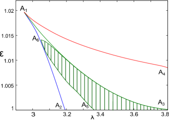
Figure 1: $\mathcal{E}$-$\lambda$ plot for quasi-spherical disc geometry ($\gamma=1.35$ and $a=0.1$)

Figure 1 shows the $\left[\mathcal{E}-\lambda\right]$ parameter space for adiabatic accretion in quasi- spherical geometry for $\left[\gamma=1.35,a=0.1\right]$. Similar diagrams can be produced for the two other geometries as well. A₁A₂A₃A₄ represents the region of $\left[{\cal E},\lambda\right]$ for which the corresponding polynomial equation in $r_{c}$ along with the corresponding critical point conditions provides three real positive roots lying outside $r_{+}$, where $r_{+}=1+\sqrt{1-a^{2}}$, $a$ being the Kerr parameter. For region A₁A₂A₃, one finds ${\dot{\Xi}}_{\rm inner}>{\dot{\Xi}}_{\rm outer}$ and accretion is multi-critical. A₃A₅A₆ (shaded in green), which is a subspace of A₁A₂A₃ allows shock formation. Such a subspace provides true multi-transonic accretion where the stationary transonic solution passing through the outer sonic point joins with the stationary transonic solution constructed through the inner sonic point through a discontinuous energy preserving shock of Rankine-Hugoniot type. Such shocked multi-transonic solution contains two smooth transonic (from sub to super) transitions at two regular sonic points (of saddle type) and a discontinuous transition (from super to sub) at the shock location.

On the other hand, the region A₁A₃A₄ represents the subset of $\left[{\cal E},\lambda,\gamma\right]_{\rm mc}$ (where ‘mc’ stands for ‘multi-critical’) for which ${\dot{\Xi}}_{\rm inner}<{\dot{\Xi}}_{\rm outer}$ and hence incoming flow can have only one critical point of saddle type and the background flow possesses one acoustic horizon at the inner saddle type sonic point. The boundary A₁A₃ between these two regions represents the value of $\left[{\cal E},\lambda,\gamma\right]$ for which multi-critical accretion is characterized by ${\dot{\Xi}}_{\rm inner}={\dot{\Xi}}_{\rm outer}$ and hence the transonic solutions passing through the inner and the outer sonic points are completely degenerate, leading to the formation of a heteroclinic orbit on the phase portrait. Such flow pattern may be subjected to instability and turbulence as well.

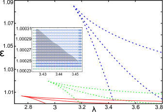
Figure 2: Comparision of $\mathcal{E}$-$\lambda$ plot for three different flow geometries ($\gamma=1.35$ and $a=0.1$). Constant height disc, quasi-spherical flow and flow in vertical hydrostatic equilibrium represented by blue dashed lines, green dotted lines and red solid lines respectively. Shaded region in the inset depicts $\left[\mathcal{E},\lambda\right]$ space overlap with multicritical solutions for all three models.

In figure 2, for the same values of $\left[\gamma,a\right]$, we compare the parameter spaces for three different flow geometries. The common region for which multiple critical points are formed for all three flow geometries are shown in the inset.

4 Classification of critical points for polytropic accretion

In the previous section, we found that the transonic accretion may possess, depending on the initial boundary conditions defined by the values of $\left[\mathcal{E},\lambda,\gamma,a\right]$, one or three critical points. Since we consider inviscid, non-dissipative flow, the critical points are expected to be either of saddle type, or of centre type. No spiral (instead of the centre type) or nodal type points may be observed. The nature of the critical points, whose locations are obtained by substituting the critical point conditions for accretion flow in different geometries and solving for the equation of specific energy, cannot be determined from such solutions. A classification scheme has been developed (Goswami et al. (2007)) to accomplish such a task. Once the location of a critical point is identified, the linearized study of the space gradients of the square of the advective velocity in the close neighbourhood of such a point may be carried out to develop a complete and rigorous mathematical classification scheme to understand whether a critical point is of saddle type, or of centre type. Such methodology is based on a local classification scheme. The global understanding of the flow topology is not possible to accomplish using such scheme. For that purpose, study of the stationary integral flow solution is necessary, which can be accomplished only numerically. Such numerical scheme to obtain the global phase portraits will be discussed in detail in the subsequent sections.

Stationary axisymmetric accretion in the Kerr metric can be described by a first order autonomous differential equation (Goswami et al. (2007)) to apply the formalism borrowed from the dynamical systems theory and to find out the nature of the critical points using such formalism. Below, we generalize such analysis for polytropic accretion in three different models.

4.1 Constant Height Flow

The gradient of square of the sound speed and the dynamical flow velocity (the advective velocity) can be written as,

$$\frac{dc_{s}^{2}}{dr}=(\gamma-1-c_{s}^{2})\left[\frac{-1}{2(1-u^{2})}\frac{du^{2}}{dr}-\frac{f^{\prime}}{2f}\right]$$ (30)

$$\frac{du^{2}}{dr}=\frac{2\left[\frac{r-1}{\Delta}c_{s}^{2}-\frac{f^{\prime}}{2f}\right]}{\frac{1}{u^{2}}\left(\frac{1}{1-u^{2}}\right)(u^{2}-c_{s}^{2})}$$ (31)

One can decompose the expression for $\frac{du^{2}}{dr}$ into two parametrized equations using a dummy mathematical parameter $\tau$ as

$$\frac{du^{2}}{d\tau}=2\left[\frac{r-1}{\Delta}c_{s}^{2}-\frac{f^{\prime}}{2f}\right]$$

$$\frac{dr}{d\tau}=\frac{1}{u^{2}}\left(\frac{1}{1-u^{2}}\right)(u^{2}-c_{s}^{2})$$ (32)

The above equation is an autonomous equation and hence $\tau$ does not explicitly appear in their right hand sides. About the fixed values of the critical points, one uses a perturbation prescription of the following form,

$$u^{2}=u_{c}^{2}+\delta u^{2}$$ (33)

$$c_{s}^{2}={c_{s}}_{c}^{2}+\delta c_{s}^{2}$$ (34)

$$r=r_{c}+\delta r$$ (35)

and derives a set of two autonomous first order linear differential equations in the $\delta r-\delta u^{2}$ plane, by expressing $\delta c_{s}^{2}$ in terms of $\delta r$ and $\delta u^{2}$ as,

$$\frac{\delta c_{s}^{2}}{{c_{s}}_{c}^{2}}=(\gamma-1-{c_{s}}_{c}^{2})\left[\frac{-1}{2u_{c}^{2}(1-u_{c}^{2})}\delta u^{2}-\frac{r_{c}-1}{\Delta_{c}}\delta r\right]$$ (36)

This form of $\delta c_{s}^{2}$ has been derived using the modified form (in terms of $u^{2}$ instead of $u$) of the mass accretion rate (eqn.(7)) and its corresponding expression for the entropy accretion rate (eqn.(8)). Through this procedure, a set of coupled linear equations in $\delta r$ and $\delta u^{2}$ will be obtained as

$$\frac{d}{d\tau}(\delta u^{2})=\mathcal{A}_{CH}\delta u^{2}+\mathcal{B}_{CH}\delta r$$ (37)

$$\frac{d}{d\tau}(\delta r)=\mathcal{C}_{CH}\delta u^{2}+\mathcal{D}_{CH}\delta r$$ (38)

where

$${\cal A}_{CH}=\dfrac{(1-r_{c})(\gamma-1-c_{s_{c}}^{2})}{\Delta_{c}(1-u_{c}^{2})}$$ (39)

$${\cal B}_{CH}=2\left[\dfrac{c_{s_{c}}^{2}}{\Delta_{c}}-\dfrac{(r_{c}-1)^{2}c_{s_{c}}^{2}}{\Delta_{c}^{2}}(\gamma+1-c_{s_{c}}^{2})\right.$$

$$\left.-\dfrac{f^{\prime\prime}}{2f}+\dfrac{1}{2}\left(\dfrac{f^{\prime}}{f}\right)^{2}\right]$$ (40)

$${\cal C}_{CH}=\left[1+\dfrac{(\gamma-1-c_{s_{c}}^{2})}{2(1-u_{c}^{2})}\right]\dfrac{1}{u_{c}^{2}(1-u_{c}^{2})}$$ (41)

$${\cal D}_{CH}=-{\cal A}_{CH}$$ (42)

Using trial solutions of the form $\delta u^{2}\sim\exp(\Omega\tau)$ and $\delta r\sim\exp(\Omega\tau)$ ($\Omega$, in this context, should not be confused with angular velocity of the flow in eqn.(5)), the eigenvalues of the stability matrix can be expressed as,

$$\Omega_{CH}^{2}\equiv\Omega_{{CH}_{1}}\Omega_{{CH}_{2}}=\mathcal{B}_{CH}\mathcal{C}_{CH}-\mathcal{A}_{CH}\mathcal{D}_{CH}$$ (43)

Once the numerical values corresponding to the location of the critical points are obtained, it is straightforward to calculate the numerical value corresponding to the expression for $\Omega^{2}$, since $\Omega^{2}$ is essentially a function of $r_{c}$. The accreting black hole system under consideration is a conservative system, hence either $\Omega^{2}>0$, which implies the critical points are saddle type, or one obtains $\Omega^{2}<0$, which implies the critical points are centre type. One thus understands the nature of the critical points (whether saddle type or centre type) once the values of $r_{c}$ is known. It has been observed that the single critical point solutions are always of saddle type. This is obvious, otherwise monotransonic solutions would not exist. It is also observed that for multi-critical flow, the middle critical point is of centre type and the inner and the outer critical points are of saddle type. This will be explicitly shown diagramatically in the subsequent sections.

4.2 Conical Flow

The gradient of square of the sound speed and the advective velocity are given by,

$$\dfrac{dc_{s}^{2}}{dr}=(\gamma-1-c_{s}^{2})\left[\dfrac{-1}{2(1-u^{2})}\dfrac{du^{2}}{dr}-\dfrac{f^{\prime}}{2f}\right]$$ (44)

$$\dfrac{du^{2}}{dr}=\dfrac{2\left[\dfrac{(2r^{2}-3r+a^{2})}{\Delta r}c_{s}^{2}-\dfrac{f^{\prime}}{2f}\right]}{\dfrac{1}{u^{2}}\left(\dfrac{1}{1-u^{2}}\right)(v^{2}-c_{s}^{2})}$$ (45)

The parametrized form of the expression of $\frac{du^{2}}{dr}$ is given by the equations,

$$\dfrac{du^{2}}{d\tau}=2\left[\dfrac{(2r^{2}-3r+a^{2})}{\Delta r}c_{s}^{2}-\dfrac{f^{\prime}}{2f}\right]$$

$$\dfrac{dr}{d\tau}=(u^{2}-c_{s}^{2})\dfrac{1}{u^{2}(1-u^{2})}$$ (46)

Using the perturbation scheme of eqns.(33), (34) and (35) we obtain,

$$\dfrac{\delta c_{s}^{2}}{c_{s_{c}}^{2}}=(\gamma-1-c_{s_{c}}^{2})\left[-\dfrac{1}{2u_{c}^{2}(1-u_{c}^{2})}\delta u^{2}\right.$$

$$\left.-\dfrac{(2r_{c}^{2}-3r_{c}+a^{2})}{\Delta_{c}r_{c}}\delta r\right]$$ (47)

where $\delta c_{s}^{2}$ has been derived using modified form of eqns.(14) and (15). The coupled linear equations in $\delta r$ and $\delta u^{2}$ are given by,

$$\dfrac{d}{d\tau}(\delta u^{2})={\cal A}_{CF}\delta u^{2}+{\cal B}_{CF}\delta r$$ (48)

$$\dfrac{d}{d\tau}(\delta r)={\cal C}_{CF}\delta u^{2}+{\cal D}_{CF}\delta r$$ (49)

where,

$${\cal A}_{CF}=-\dfrac{(2r_{c}^{2}-3r_{c}+a^{2})(\gamma-1-c_{s_{c}}^{2})}{\Delta_{c}r_{c}(1-u_{c}^{2})}$$ (50)

$${\cal B}_{CF}=\dfrac{2(4r_{c}-3)c_{s_{c}}^{2}}{\Delta_{c}r_{c}}-\dfrac{f^{\prime\prime}}{f}+\left(\dfrac{f^{\prime}}{f}\right)^{2}-\dfrac{2c_{s_{c}}^{2}}{\Delta_{c}^{2}r_{c}^{2}}(2r_{c}^{2}-3r_{c}+a^{2})$$

$$\left[(3r_{c}^{2}-4r_{c}+a^{2})+(\gamma-1-c_{s_{c}}^{2})(2r_{c}^{2}-3r_{c}+a^{2})\right]$$ (51)

$${\cal C}_{CF}=\left[1+\dfrac{(\gamma-1-c_{s_{c}}^{2})}{2(1-u_{c}^{2})}\right]\dfrac{1}{u_{c}^{2}(1-u_{c}^{2})}$$ (52)

$${\cal D}_{CF}=-{\cal A}_{CF}$$ (53)

Using the prescription mentioned in the previous subsection, eigenvalues of the stability matrix are obtained as,

$$\Omega_{CF}^{2}\equiv\Omega_{{CF}_{1}}\Omega_{{CF}_{2}}=\mathcal{B}_{CF}\mathcal{C}_{CF}-\mathcal{A}_{CF}\mathcal{D}_{CF}$$ (54)

4.3 Flow in hydrostatic equilibrium along the vertical direction

The gradient of square of the advective velocity is given by,

$$\dfrac{du^{2}}{dr}=\frac{\beta^{2}c_{s}^{2}\left[\dfrac{F_{1}^{\prime}}{F_{1}}-\dfrac{1}{F}\dfrac{\partial F}{\partial r}\right]-\dfrac{f^{\prime}}{f}}{\left(1-\frac{\beta^{2}c_{s}^{2}}{u^{2}}\right)\dfrac{1}{(1-u^{2})}+\dfrac{\beta^{2}c_{s}^{2}}{F}\left(\dfrac{\partial F}{\partial u^{2}}\right)}$$ (55)

where $F_{1}=\Delta r^{4}$ and $\beta=\sqrt{\frac{2}{\gamma+1}}$.
The parametrized form of the expression of $\frac{du^{2}}{dr}$ is given by the equations,

$$\dfrac{du^{2}}{d\tau}=\beta^{2}c_{s}^{2}\left[\dfrac{F_{1}^{\prime}}{F_{1}}-\dfrac{1}{F}\dfrac{\partial F}{\partial r}\right]-\dfrac{f^{\prime}}{f}$$

$$\dfrac{dr}{d\tau}=\left(1-\frac{\beta^{2}c_{s}^{2}}{u^{2}}\right)\dfrac{1}{(1-u^{2})}+\dfrac{\beta^{2}c_{s}^{2}}{F}\left(\dfrac{\partial F}{\partial u^{2}}\right)$$ (56)

Using the perturbation scheme of eqns.(33), (34) and (35), and modified forms of eqns.(21) and (23) we obtain,

$$\frac{\delta c_{s}^{2}}{c_{s_{c}}^{2}}=\mathcal{A}\delta u^{2}+\mathcal{B}\delta r$$ (57)

where,
$\mathcal{A}=-\frac{\gamma-1-c_{s_{c}}^{2}}{\gamma+1}\left[\frac{1}{u_{c}^{2}\left(1-u_{c}^{2}\right)}-\frac{1}{F_{c}}\left(\frac{\partial F}{\partial u^{2}}\right)\bigg{|}_{c}\right]$,
$\mathcal{B}=-\frac{\gamma-1-c_{s_{c}}^{2}}{\gamma+1}\left[\frac{F_{1}^{\prime}(r_{c})}{F_{1}(r_{c})}-\frac{1}{F_{c}}\left(\frac{\partial F}{\partial r}\right)\bigg{|}_{c}\right]$.
The coupled linear equations in $\delta r$ and $\delta u^{2}$ are given by,

$$\frac{\mathrm{d}}{{\mathrm{d}}\tau}(\delta u^{2}) = \beta^{2}c_{\mathrm{sc}}^{2}\left[\frac{{\mathcal{A}}F_{1}^{\prime}}{F_{1}}-\frac{\mathcal{AC}}{F}+\frac{\mathcal{CD}}{F^{2}}-\frac{\Delta_{3}}{F}\right]\,\delta u^{2}+\left[\frac{\beta^{2}c_{\mathrm{sc}}^{2}F_{1}^{\prime}}{F_{1}}\left\{{\mathcal{B}}+\left(\frac{F_{1}^{\prime\prime}}{F_{1}^{\prime}}-\frac{F_{1}^{\prime}}{F_{1}}\right)\right\}\right.$$ (58)

$$\left.-\frac{f^{\prime}}{f}\left(\frac{f^{\prime\prime}}{f^{\prime}}-\frac{f^{\prime}}{f}\right)-\frac{\beta^{2}c_{\mathrm{sc}}^{2}{\mathcal{C}}}{F}\left({\mathcal{B}}-\frac{\mathcal{C}}{F}+\frac{\Delta_{4}}{\mathcal{C}}\right)\right]\delta r$$

$$\frac{{\mathrm{d}}}{{\mathrm{d}}\tau}(\delta r) = \left[\frac{1}{\left(1-u_{\mathrm{c}}^{2}\right)^{2}}-\frac{\beta^{2}c_{\mathrm{sc}}^{2}}{u_{\mathrm{c}}^{2}\left(1-u_{\mathrm{c}}^{2}\right)}\left\{{\mathcal{A}}+\frac{2u_{\mathrm{c}}^{2}-1}{\left(1-u_{\mathrm{c}}^{2}\right)^{2}}\right\}+\frac{\beta^{2}c_{\mathrm{sc}}^{2}{\mathcal{D}}}{F}\left({\mathcal{A}}-\frac{\mathcal{D}}{F}+\frac{\Delta_{1}}{\mathcal{D}}\right)\right]\delta u^{2}$$ (59)

$$+\left[-\frac{\beta^{2}c_{\mathrm{sc}}^{2}{\mathcal{B}}}{u_{\mathrm{c}}^{2}\left(1-u_{\mathrm{c}}^{2}\right)}+\frac{\beta^{2}c_{\mathrm{sc}}^{2}{\mathcal{D}}}{F}\left({\mathcal{B}}-\frac{\mathcal{C}}{F}+\frac{\Delta_{2}}{\mathcal{D}}\right)\right]\delta r$$

where,
$\mathcal{C}=\left(\frac{\partial F}{\partial r}\right)\bigg{|}_{c}$, $\mathcal{D}=\left(\frac{\partial F}{\partial u^{2}}\right)\bigg{|}_{c}$,
$\Delta_{1}=\frac{\partial}{\partial u^{2}}\left(\frac{\partial F}{\partial u^{2}}\right)\bigg{|}_{c}$, $\Delta_{2}=\frac{\partial}{\partial r}\left(\frac{\partial F}{\partial u^{2}}\right)\bigg{|}_{c}$, $\Delta_{3}=\frac{\partial}{\partial u^{2}}\left(\frac{\partial F}{\partial r}\right)\bigg{|}_{c}$, $\Delta_{4}=\frac{\partial}{\partial r}\left(\frac{\partial F}{\partial r}\right)\bigg{|}_{c}$.
Using the prescription mentioned in the previous subsection, eigenvalues of the stability matrix are obtained as,

$$\Omega_{VE}^{2}=\beta^{4}c_{s_{c}}^{4}\chi^{2}+\xi_{1}\xi_{2}$$ (60)

where, $\chi=\left[\frac{F_{1}^{\prime}{\mathcal{A}}}{F_{1}}-\frac{\mathcal{AC}}{F}+\frac{\mathcal{CD}}{F^{2}}-\frac{\Delta_{3}}{F}\right]=\left[\frac{\mathcal{B}}{u_{\mathrm{c}}^{2}\left(1-u_{\mathrm{c}}^{2}\right)}-\frac{\mathcal{BD}}{F}+\frac{\mathcal{CD}}{F^{2}}-\frac{\Delta_{2}}{F}\right]$,
$\xi_{1}=\frac{\beta^{2}c_{\mathrm{sc}}^{2}F^{\prime}_{1}}{F_{1}}\left[{\mathcal{B}}+\frac{F_{1}^{\prime\prime}}{F_{1}^{\prime}}-\frac{F_{1}^{\prime}}{F_{1}}\right]-\frac{f^{\prime}}{f}\left[\frac{f^{\prime\prime}}{f^{\prime}}-\frac{f^{\prime}}{f}\right]-\frac{\beta^{2}c_{\mathrm{sc}}^{2}\mathcal{C}}{F}\left[{\mathcal{B}}-\frac{\mathcal{C}}{F}+\frac{\Delta_{4}}{\mathcal{C}}\right]$, and
$\xi_{2}=\frac{1}{\left(1-u_{\mathrm{c}}^{2}\right)^{2}}-\frac{\beta^{2}c_{\mathrm{sc}}^{2}}{u_{\mathrm{c}}^{2}\left(1-u_{\mathrm{c}}^{2}\right)}\left[{\mathcal{A}}+\frac{2u_{\mathrm{c}}^{2}-1}{u_{\mathrm{c}}^{2}\left(1-u_{\mathrm{c}}^{2}\right)}\right]+\frac{\beta^{2}c_{\mathrm{sc}}^{2}\mathcal{D}}{F}\left[\mathcal{A}-\frac{\mathcal{D}}{F}+\frac{\Delta_{1}}{\mathcal{D}}\right]$.

5 Dependence of $\Omega^{2}$ on flow and spin parameters for polytropic accretion with various matter geometries

In the previous section, we derived the explicit analytical expressions for calculating the numerical values of $\Omega^{2}$ once the locations of the critical points are known. We also argued that the solutions corresponding to multi-transonic accretion consist of three critical points- one of centre type and the other two of saddle type. In order to represent a real multi-transonic flow, the middle critical point is required to be of centre type such that the actual physical flow occurs through the inner and outer critical points, which are required to be of saddle type in nature. In terms of the present analytical formalism, $\Omega^{2}$ corresponding to the inner and outer critical points must assume a positive numerical value, whereas those corresponding to the middle critical points must be negative. Figs. 3, 4 and 5 establish the validity of this requirement.

Figure 3: Comparison of $\Omega^{2}$ vs. $\left[\mathcal{E},\lambda\right]$ of the inner and outer critical points for constant height flow (CH), quasi-spherical flow (CF) and flow in vertical hydrostatic equilibrium (VE) ($\gamma=1.35$, $a=0.1$).

Figure 4: Comparison of $\Omega^{2}$ vs. $\left[\mathcal{E},\lambda\right]$ of the middle critical point for constant height flow (CH), quasi-spherical flow (CF) and flow in vertical hydrostatic equilibrium (VE) ($\gamma=1.35$, $a=0.1$).

In fig. 3, the variation of $\Omega^{2}$ for inner and outer critical points has been depicted over the entire physically accessible domain of $\left[\mathcal{E},\lambda\right]$ for a given value of $\left[\gamma=1.35,a=0.1\right]$. As predicted, the numerical values are all positive, indicating a saddle nature. A similar observation is made in fig. 4 where the values of $\Omega^{2}$ for the middle critical points over the entire domain of $\left[\mathcal{E},\lambda\right]$ with the same values of the other flow parameters, are negative, indicating a stable point of centre type in nature. An immediate comparision can be made between the absolute magnitudes of $\Omega^{2}$ for the inner and outer critical points. It is interesting to note that $\Omega^{2}_{inner}>>\Omega^{2}_{outer}$ indicating a correlation between numerical value of the quantity and the influence of gravity due to the central accretor, not only propagated through the value of metric components at the point, but also through the dynamical and thermodynamic variables pertaining to the flow. However, it is too far fetched to comment on any physical realization of the quantity at hand as we are dealing with a highly nonlinear system with a large number of parameters and variables with complicated implicit dependence on one another. It is only safe to state that the sign of the quantity is all that we are interested in at present, to understand the nature of the critical points in order to visualize the phase space orbits, without delving into actual numerics. A comparision of the three different flow geometries reveals that $|\Omega^{2}|_{CH}>|\Omega^{2}|_{CF}>|\Omega^{2}|_{VE}$.

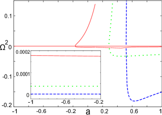
Figure 5: Comparison of $\Omega^{2}$ vs. $a$ for constant height flow (blue dashed lines), quasi-spherical flow (green dotted lines) and flow in vertical hydrostatic equilibrium (red solid lines)($\gamma=1.35$, $\mathcal{E}=1.003$, $\lambda=3.0$). Inset shows a magnified view of the common monotransonic region for the three flow geometries.

Fig. 5 provides an elegant pictorial method of realizing the nature of accretion over the entire range of black hole spin for a given value of specific energy and specific angular momentum of the flow at a particular polytropic index ($\mathcal{E}=1.003,\lambda=0.3,\gamma=1.35$). The region with a single positive value of $\Omega^{2}$ (shown in inset) represents a saddle type critical point indicating at monotransonic flow for all three geometric configurations. The single positive value is then observed to split into one negative value and two positive values indicating the formation of one centre type middle critial point and two saddle type critical points. One of the two saddle points with its numerical value comparable with that of the single saddle type point in the monotransonic region represents the outer critical point, while the other with a higher value represents the inner critical point which is closer to the event horizon. It appears as if a saddle-centre pair is generated from the initial saddle at a particular value of spin and as one moves towards higher values of black hole spin, the new saddle, i.e. the inner critical point moving closer and closer to the horizon begins assuming higher values of $\Omega^{2}$ until it crosses the horizon and ultimately disappears from the physically accessible regime. And finally, one is left with the centre type middle critical point through which no physical flow can occur, and the previous saddle type outer critical point through which accretion continues as a purely monotransonic flow. The same universal trend can be observed in all three disc structures although splitting occurs at different values of $a$ and the relative magnitudes of $\Omega^{2}$ are distinct for each flow geometry. It is to be noted that for the same energy and angular momentum of the accreting fluid, flow in the hydrostatic equilibrium along the vertical direction allows for multitransonic solutions at the lowest values of black hole spin (even for counter-rotating black holes in the given case). It may also be observed that since the values of $\Omega^{2}$ represent critical points of a system, the splitting actually corresponds to a super-critical pitchfork bifurcation in the theory of dynamical systems where a stable critical point bifurcates into two stable critical points (inner and outer in this case through which actual flow occurs) and an unstable critical point (middle centre type point through which physical flow in not allowed).

6 Integral flow solutions with shock for polytropic accretion

In the previous section, one finds that it is possible to understand the nature of the critical points through some local stability analysis, i.e., the methodology is applicable in the close neighbourhood of the critical points. The global nature of the flow topology, however, is possible to know only through the stationary integral solutions of the corresponding flow equations. Such integral solutions are obtained through numerical techniques. For a particular set of values of $\left[\mathcal{E},\lambda,\gamma,a\right]$, one calculates the location of critical point(s). The values of $\left[u,c_{s},\frac{du}{dr},\frac{dc_{s}}{dr}\right]$ on such critical points are then computed. Starting from the critical point, the expressions corresponding to $\frac{du}{dr}$ and $\frac{dc_{s}}{dr}$ are then numerically solved to obtain the radial Mach number vs. radial distance profile. For transonic flow with multiple critical points, a stationary shock may form. For such flow, integral stationary subsonic solutions pass through the outer sonic point (associated with the saddle type outer critical point) and becomes supersonic. The supersonic flow then encounters a discontinuous transition through shock and becomes subsonic once again. The location of the shock has to be determined by solving the corresponding shock conditions. The post-shock subsonic flow then passes through the inner sonic point (corresponding to the saddle type inner critical point) to become supersonic again and ultimately plunge into the event horizon.

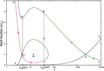
Figure 6: Phase space portrait (Mach number vs. $r$ plot) for quasi-spherical disc ($\mathcal{E}=1.0003$, $\lambda=3.5$, $\gamma=1.35$, $a=0.1$). $r_{\rm sh}^{\rm in}=4.805$, $r_{\rm sh}^{\rm out}=38.15$, $r^{\rm in}=4.5$ (inner sonic point $I$), $r^{\rm mid}=13.712$ (mid sonic point $M$), $r^{\rm out}=2244.313$ (outer sonic point $O$).

Figure 6 shows the Mach number vs radial distance phase portrait of a shocked multi-transonic flow for accretion in quasi-spherical geometry. Branch $AOB$ (green curve) represents accretion through the outer sonic point $O$. The flow encounters a stable, standing, energy preserving shock at $r=r_{\rm sh}^{\rm out}$ whose location is obtained by using the numerical scheme of equating shock-invariant quantities (elaborated in the next subsection). It then jumps along the line of discontinuity $BC$ (blue dashed line). Thus being transformed into a subsonic, compressed and hotter flow, it then approaches the event horizon moving along the line $CC^{\prime}ID$ (red curve) and becoming supersonic once again while passing through the inner sonic point $I$. $B^{\prime}C^{\prime}$ shows an unstable line of discontinuity which is inaccessible to physical flow. $FOE$ represents the corresponding wind solution, while $DIC^{\prime}CF$ is a homoclinic orbit encompassing the middle critical point $M$.

6.1 Shock-invariant quantities ($S_{\rm h}$)

The shock-invariant quantity ($S_{\rm h}$) is defined as a quantity whose numerical value remains the same on the integral solution branch passing through the outer sonic point as well as the branch passing through the inner sonic point, exclusively at the location(s) of physically allowed discontinuities obeying the general relativistic Rankine Hugoniot conditions. Thus, once expression for the shock-invariant quantities are obtained, the corresponding shock locations can be evaluated by numerically checking for the condition $S_{\rm h}^{\rm out}=S_{\rm h}^{\rm in}$, where $S_{\rm h}^{\rm out}$ and $S_{\rm h}^{\rm in}$ are the shock-invariant quantities defined on the integral flow solutions passing through the outer and the inner sonic points respectively. The Rankine Hugoniot conditions applied to a fully general relativistic background flow are given by,

$$\left[\left[\rho u^{\mu}\right]\right]=0\text{, and }\left[\left[T^{\mu\nu}\right]\right]=0$$ (61)

where $\left[\left[V\right]\right]=V_{-}-V_{+}$, $V_{+}$ and $V_{-}$ symbolically denote the values of some flow variable $V$ before and after the shock respectively.
Eqn.(61) can further be decomposed into the following three conditions,

$$\left[\left[\rho u^{r}\right]\right]=0,$$ (62)

$$\left[\left[(p+\epsilon)u_{t}u^{r}\right]\right]=0,$$ (63)

$$\left[\left[(p+\epsilon)u^{r}u^{r}+p\right]\right]=0,$$ (64)

where $u^{r}=\frac{u\Delta^{\frac{1}{2}}}{r\sqrt{1-u^{2}}}$.
Using the definition for specific enthalpy ($h$) of the fluid given by,

$$h=\frac{p+\epsilon}{\rho}$$ (65)

and using eqn.(2) and eqn.(4) together with the polytropic equation of state $p=K\rho^{\gamma}$, one can express $\rho$, $p$ and $\epsilon$ in terms of the adiabatic sound speed $c_{s}^{2}$ as,

$$\rho=\left[\frac{c_{s}^{2}(\gamma-1)}{K\gamma(\gamma-1-c_{s}^{2})}\right]^{\frac{1}{\gamma-1}}$$

$$p=K^{\frac{-1}{\gamma-1}}\left[\frac{c_{s}^{2}(\gamma-1)}{\gamma(\gamma-1-c_{s}^{2})}\right]^{\frac{\gamma}{\gamma-1}}$$

$$\epsilon=\left(\frac{c_{s}^{2}(\gamma-1)}{K\gamma(\gamma-1-c_{s}^{2})}\right)^{\frac{1}{\gamma-1}}\left[1+\frac{1}{\gamma}\left(\frac{c_{s}^{2}}{\gamma-1-c_{s}^{2}}\right)\right]$$ (66)

Now, considering geometry of the flow eq.(62) can be re-written as

$$\left[\left[\rho u^{r}\mathcal{H}(r)\right]\right]=0$$ (67)

where, the accretion geometry dependent terms $\mathcal{H}(r)$ for three different flow structures are given by,

$$\mathcal{H}_{CH}(r)=2\pi rH$$

$$\mathcal{H}_{CF}(r)=\Theta r^{2}$$

$$\mathcal{H}_{VE}(r)=4\pi rH(r)$$ (68)

$H$ being the thickness of the constant height disc, $\Theta$ being the solid angle subtended by the quasi-spherical disc at the horizon and $H(r)$ being the radius dependent thickness for flow in hydrostatic equilibrium along the vertical direction given by eq.(22).
Substituting eqs.(68) and (66) in eqs.(67) and (64), and then solving simultaneously, we derive the shock-invariant quantitites ($S_{h}$) for all three flow geometries as,

$$S_{h}\bigg{|}_{CH}=\frac{u^{2}(\gamma\frac{\Delta}{r^{2}}-c_{s}^{2})+c_{s}^{2}}{u\sqrt{1-u^{2}}(\gamma-1-c_{s}^{2})}$$ (69)

$$S_{h}\bigg{|}_{CF}=\frac{u^{2}(\gamma\frac{\Delta}{r^{2}}-c_{s}^{2})+c_{s}^{2}}{u\sqrt{1-u^{2}}(\gamma-1-c_{s}^{2})}$$ (70)

$$S_{h}\bigg{|}_{VE}=\frac{\sqrt{F}\{u^{2}(\gamma\frac{\Delta}{r^{2}}-c_{s}^{2})+c_{s}^{2}\}}{uc_{s}\sqrt{(1-u^{2})(\gamma-1-c_{s}^{2})}}$$ (71)

7 Shock parameter space for polytropic accretion

We now intend to see which region of the $\left[\mathcal{E}-\lambda\right]$ parameter space allows shock formation. For a fixed set of $\left[\gamma=1.35,a=0.57\right]$, we check the validity of the Rankine Hugoniot condition corresponding to every value of $\left[\mathcal{E},\lambda\right]$ for which the accretion flow possesses three critical points. This means the shock-invariant quantity is calculated for every $\left[\mathcal{E},\lambda\right]$ for which the multitransonic accretion is possible, and it is observed that the quantities calculated along the solution passing through the outer and the inner sonic points become equal at a particular radial distance, i.e. at the shock location, only for a subset of such $\left[\mathcal{E},\lambda\right]$. We then plot the corresponding $\left[\mathcal{E},\lambda\right]_{\rm{shock}}$ for various geometric configurations of matter.

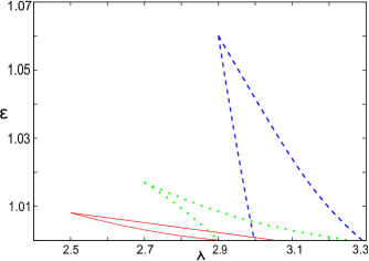
Figure 7: Comparision of $\mathcal{E}$-$\lambda$ plot of allowed shocked multitransonic accretion solutions for three different flow geometries ($\gamma=1.35$ and $a=0.57$). Constant height disc, quasi-spherical flow and flow in vertical hydrostatic equilibrium represented by blue dashed lines, green dotted lines and red solid lines respectively.

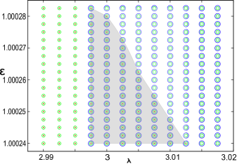
Figure 8: Shaded region depicts the common domain of $\left[\mathcal{E},\lambda\right]$ ($\gamma=1.35,a=0.57$) which allows shock formation in constant height disc (blue circles), quasi-spherical disc (green circles) and flow in hydrostatic equilibrium (red dots).

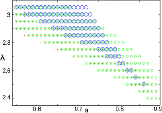
Figure 9: Overlap region of $\left[a,\lambda\right]$ ($\gamma=1.35,\mathcal{E}=1.00024$) which allows shock formation in constant height disc (blue circles), quasi-spherical disc (green circles) and flow in hydrostatic equilibrium (red dots).

In fig. 7 we plot such shock forming parameter space for three different flow geometries. The shock forming region of $\left[\mathcal{E},\lambda\right]$ for a relevant combination of $a$ and $\gamma$, which is common to all three geometries is shown in fig. 8. Similarly, fig. 9 shows the domain of $\left[a,\lambda\right]$ for a given value of $\mathcal{E}$ and $\gamma$ where shock forming regions of the three flow models overlap. This particular plot indicates at the requirement of an anti-correlation between the angular momentum of flow and spin of the central gravitating source for multitransonic accretion to occur. Moreover, it may be observed that a higher difference between these two values allows for a greater multitransonic shock forming region. The only probable reason behind this typical observation seems to be an increase in the effective centrifugal barrier experienced by the flow. These overlapping parameter space domains are of extreme importance for our purpose. All the shock related flow properties for which the flow behaviour is to be compared for three different geometries, are to be characterized by $\left[\mathcal{E},\lambda,\gamma,a\right]$ corresponding to these common regions only. We will show this in greater detail in subsequent sections.

In what follows, we will study the dependence of the shock location ($r_{sh}$), shock strength (the ratio of pre to post shock values of the Mach number, $M_{+}/M_{-}$), shock compression ratio (the ratio of the post to pre shock matter density, $\rho_{-}/\rho_{+}$), the ratio of post to pre shock temperature ($T_{-}/T_{+}$) and pressure ($P_{-}/P_{+}$), on the black hole spin parameter $a$. Subscripts ‘+’ and ‘-’ represent pre and post shock quantities respectively. One can study the dependence of such quantities on other accretion parameters, i.e. $\left[\mathcal{E},\lambda,\gamma\right]$ as well. Such dependence, however, are not much relevant for our study in this work, since for a fixed value of the Kerr parameter, nature of such dependence should actually be equivalent to the corresponding nature of the dependence of $\left[r_{sh},M_{+}/M_{-},\rho_{-}/\rho_{+},P_{-}/P_{+}\right]$ on $\left[\mathcal{E},\lambda,\gamma\right]$ as observed in the Schwarzschild metric which has already been investigated in P1. Hereafter, throughout this work, we will study the dependence of every physical quantity on the Kerr parameter only, for a fixed set of $\left[\mathcal{E},\lambda,\gamma\right]$.

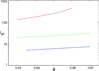
Figure 10: Shock location ($r_{sh}$) vs. $a$ plot ($\gamma=1.35,\mathcal{E}=1.00024,\lambda=2.9$) for constant height disc (dashed blue line), quasi-spherical disc (dotted green line) and flow in hydrostatic equilibrium (solid red line).

Fig. 10 depicts variation of the shock location ($r_{sh}$) with spin parameter $a$. The value of $\lambda$ in this figure and all subsequent figures illustrating other shock related quantities has been chosen from the common region in fig. 9 so as to ensure the maximum possible overlapping range of $a$ permissible for shocked accretion at the given value of $\mathcal{E}$ and $\gamma$ for all three flow models. The shock location is observed to shift further from the horizon as the black hole spin increases. This is what we may expect as increasing Kerr parameter for a fixed angular momentum of the flow implies growth in the difference of the two parameters, thus strengthening the effective centrifugal barrier. Thus transonicity and shock formation are speculated to occur in earlier phases of the flow at greater distances from the massive central source. A comparision of the models reveals the following trend at a given value of $a$, $r_{sh}(VE)>r_{sh}(CF)>r_{sh}(CH)$. This indicates at the fact that flow in hydrostatic equilibrium has to face much more opposition than the other two disc geometries for the same amount of impediment posed by rotation of the flow and that of the black hole.

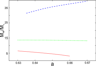
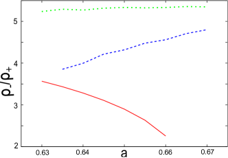
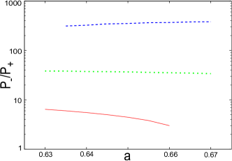
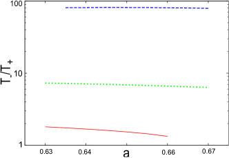
Figure 11: Variation of shock strength ($M_{+}/M_{-}$), compression ratio ($\rho_{-}/\rho_{+}$), pressure ratio ($P_{-}/P_{+}$) and temperature ratio ($T_{-}/T_{+}$) with black hole spin parameter $a$ ($\gamma=1.35,\mathcal{E}=1.00024,\lambda=2.9$) for constant height flow (dashed blue lines), quasi-spherical flow (dotted green lines) and flow in hydrostatic equilibrium (solid red lines). Subscripts ‘+’ and ‘-’ represent pre and post shock quantities respectively.

It is also interesting to note from fig. 11 that not only does the vertical equilibrium model experience maximum hindrance due to rotation, but it also exhibits the formation of shocks with the weakest strength, i.e. pre-shock to post-shock ratio of the Mach number ($M_{+}/M_{-}$), when compared with the other two models. The shocks are strongest in case of discs with a constant height and intermediate in the case of quasi-spherical flows. The strengths are observed to decrease with $a$. This might be explained by the dependence of shock location on the spin parameter. Greater values of $r_{sh}$ point at decreasing curvature of physical space-time leading to diminishing influence of gravity. Thus dropping of shock strength with increasing $a$, or in other words, higher values of $r_{sh}$, establishes that weaker gravity amounts to the formation of weaker discontinuities in the flow and vice versa. Naturally, waning shock strengths in turn lead to lower post to pre-shock compression ($\rho_{-}/\rho_{+}$), pressure ($P_{-}/P_{+}$) and temperature ($T_{-}/T_{+}$) ratios, as observed in the figure. A seemingly anomalous behaviour is observed in this context for the constant height flow geometry, in which case, in spite of an outward shifting of the shock location, shock strength is seen to increase, although behaviour of the other related ratios fall in line with our previous arguments. We shall try to discuss the reason behind such an anomaly, in the next section.

8 Quasi-terminal values

Accreting matter manifests extreme behaviour before plunging through the event horizon because it experiences the strong curvature of space-time close to the black hole. The spectral signature of such matter corresponding to that length scale helps to understand the key features of the strong gravity space-time to the close proximity of the horizon. It may also help to study the spectral signature of black hole spin. The corresponding spectral profiles and the light curves may be used for constructing the relevant black hole shadow images (Falcke et al. (2000),Takahashi (2004),Huang et al. (2007),Hioki and Maeda (2009),Zakharov et al. (2012),Straub et al. (2012)).
For a very small positive value of $\delta$ ($\sim 0.0001$), any accretion variable $V_{\delta}$ measured at a radial distance $r_{\delta}=r_{+}+\delta$ will be termed as ‘quasi-terminal value’ of that corresponding accretion variable. In Das et al. (2015), dependence of $V_{\delta}$ on the Kerr parameter was studied for polytropic accretion flow in hydrostatic equilibrium along the vertical direction. In the present work, we intend to generalize such work by computing the $V_{\delta}$ for all three different matter geometries. This generalization will be of paramount importance in understanding the geometric configuration of matter flow close to the horizon through the imaging of the shadow.
In what follows, we will study the dependence of $\left[M,\rho,T,P\right]_{r_{\delta}}$ on the Kerr parameter for shocked multi-transonic accretion in three different flow geometries to understand how the nature of such dependence gets influenced by the flow structure. We will also study such dependence for monotransonic flows for the entire range of Kerr parameters, starting from $-1$ to $+1$, to study whether any general asymmetry exists between co-rotating and counter-rotating accretion in connection to values of the corresponding $V_{\delta}$.

8.1 Dependence of $\left[M,T,\rho,P\right]_{r_{\delta}}$ on $a$ for shocked polytropic accretion

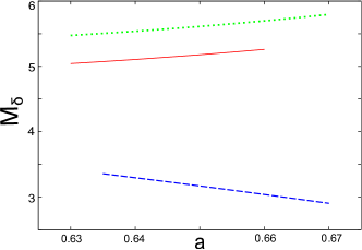
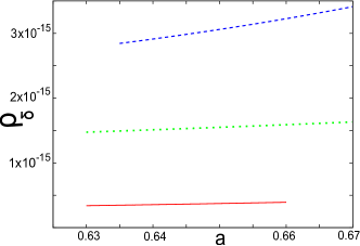
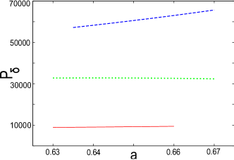
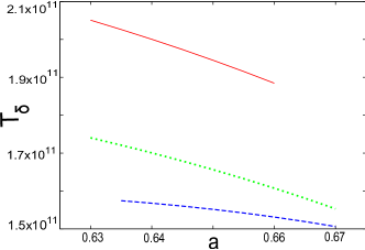
Figure 12: Variation of quasi-terminal values of Mach number ($M_{\delta}$), density ($\rho_{\delta}$), pressure ($P_{\delta}$) and temperature ($T_{\delta}$) with $a$ ($\gamma=1.35,\mathcal{E}=1.00024,\lambda=2.9$) for constant height flow (dashed blue lines), quasi-spherical flow (dotted green lines) and flow in hydrostatic equilibrium (solid red lines). Density and pressure are in CGS units of $g$ $cm^{-3}$ and $dyne$ $cm^{-2}$ respectively and temperature is in absolute units of Kelvin.

Fig. 12 demonstrates how the quasi-terminal values pertaining to Mach number ($M_{\delta}$), density ($\rho_{\delta}$), pressure ($P_{\delta}$) and the bulk ion temperature ($T_{\delta}$) vary with black hole spin $a$, at a given set of $\left[\mathcal{E},\lambda,\gamma\right]$ chosen such that a substantial range of $a$ is available for studying any observable trend of variation in the common shock regime for all three matter configurations. It might be noted that although a general course of dependence of the values may be observed within a local set of flow parameters for each geometry separately, however it is impossible to conclude upon any global trends of such sort. This is primarily due to the reason that each permissible set of $\left[\mathcal{E},\lambda,\gamma\right]$ offers an exclusively different domain of black hole spin for multitransonic accretion to occur and an even narrower common window for the viability of general relativistic Rankine Hugoniot type shocks in different geometric configurations of the flow. Hence, in spite of the fact that physical arguments may be able to specifically establish the observed results in certain cases, as it could be done with results obtained in the previous sections, however similar specific attempts made in all cases globally may not only turn out to be futile, but also dangerously misleading. The anomaly which was pointed out in the preceding section, is a stark example of such an instance. However, there is absolutely no reason for disbelief in the universality or the validity of previous physical arguments. It is only that nature offers a few selected cases to provide us the opportunity of peeking into its global behaviour. We present exactly such a case in the following subsection.

8.2 Dependence of $\left[M,T,\rho,P\right]_{r_{\delta}}$ on $a$ for monotransonic accretion

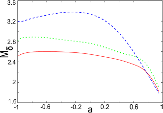
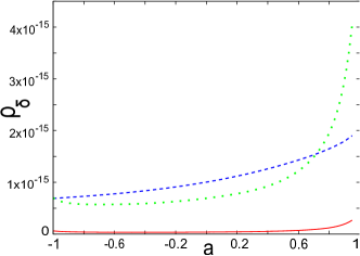
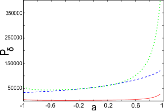
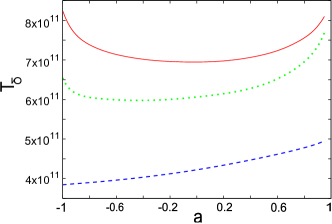
Figure 13: Variation of quasi-terminal values of Mach number ($M_{\delta}$), density ($\rho_{\delta}$), pressure ($P_{\delta}$) and temperature ($T_{\delta}$) with $a$ ($\gamma=1.35,\mathcal{E}=1.2,\lambda=2.0$) for monotransonic accretion in constant height flow (dashed blue lines), quasi-spherical flow (dotted green lines) and flow in hydrostatic equilibrium (solid red lines). Density and pressure are in CGS units of $g$ $cm^{-3}$ and $dyne$ $cm^{-2}$ respectively and temperature is in absolute units of Kelvin.

In fig. 13 we show the dependence of quasi-terminal values on black hole spin for monotransonic accretion. It is observed that weakly rotating and substantially hot flows allow for stationary monotransonic solutions over the entire range of Kerr parameters. From a careful glance at the results it becomes clear that reason behind the previously stated anomaly in general spin dependent behaviour of the corresponding physical quantities for three different flow geometries is essentially due to intrinsic limitations in the possibility of observing their variation over the complete range of spin. Since, for any given set of $\left[\mathcal{E},\lambda,\gamma\right]$, shocked stationary multitransonic accretion solutions for all matter configurations are allowed over a considerably small overlapping domain of $a$, one is able to look only through a narrow slit of the whole window. It is clearly evident from fig. 13 that the quasi-terminal values indeed exhibit common global trends of variation over $a$ for all three geometric configurations. However, while concentrating upon a small portion of spin, asymmetry in the distribution of such trends leads to crossovers and apparently non-correlative or anti- correlative mutual behaviours among the various flow models. Hence it is natural to question the utility of results with such constraints at the intrinsic level. But it is this very asymmetry, that turns out to be of supreme importance in pointing towards a prospective observational signature of the black hole spin.

9 Isothermal flow structures for various matter geometries

The equation of state characterising isothermal fluid flow is given by,

$$p=c_{s}^{2}\rho=\frac{\cal R}{\mu}\rho T=\frac{k_{B}\rho T}{\mu m_{H}}$$ (72)

where $T$ is the bulk ion temperature, $\cal R$ is the universal gas constant, $k_{B}$ is Boltzmann constant, $m_{H}$ is mass of the Hydrogen atom and $\mu$ is the mean molecular mass of fully ionized hydrogen. The temperature $T$ as introduced in the above equation, and which has been used as one of the parameters to describe the isothermal accretion, is the temperature-equivalent of the bulk ion flow velocity. That is the reason why the value appears to be high ($10^{10-11}$ K) in this work. The actual disc temperature is the corresponding electron temperature, which should be of the of the order of $10^{6-7}$ Kelvin. The electron temperature may be computed from the corresponding ion temperature by incorporating various radiative processes, see, e.g. Esin et al. (1997). These calculations for our general relativistic model are, however, beyond the scope of this particular work and will be reported elsewhere. For low angular momentum shocked flow under the influence of the Paczyński and Wiita pseudo-Schwarzschild black hole potential (Paczyński and Wiita (1980)), such computations have been performed, see, e.g. Moscibrodzka et al. (2006), as well as Czerny et al. (2007).
The energy-momentum conservation equation obtained by setting the 4-divergence (covariant derivative w.r.t. $\nu$) of eqn.(1) to be zero is,

$$p_{,\nu}(g^{\mu\nu}+v^{\mu}v^{\nu})+(p+\epsilon)v^{\nu}v^{\mu}_{;\nu}=0$$ (73)

Using eqn.(72), the general relativistic Euler equation for isothermal flow becomes,

$$\frac{c_{s}^{2}}{\rho}\rho_{,\nu}(g^{\mu\nu}+v^{\mu}v^{\nu})+v^{\nu}v^{\mu}_{;\nu}=0$$ (74)

Using the irrotationality condition $\omega_{\mu\nu}=0$, where $\omega_{\mu\nu}=l^{\lambda}_{\mu}l^{\sigma}_{\nu}v_{\left[\lambda;\sigma\right]}$,
$\omega_{\mu\nu}$ being the vorticity of the fluid, $l^{\lambda}_{\mu}$ being the projection operator in the normal direction of $v^{\mu}$
$l^{\lambda}_{\mu}=\delta^{\lambda}_{\mu}+v^{\lambda}v_{\mu}$, and $v_{\left[\lambda;\sigma\right]}=\frac{1}{2}\left(v_{\sigma;\lambda}-v_{\lambda;\sigma}\right)$, we obtain,

$$\partial_{\nu}(v_{\mu}\rho^{c_{s}^{2}})-\partial_{\mu}(v_{\nu}\rho^{c_{s}^{2}})=0$$ (75)

Taking the time component, we thus observe that for an irrotational isothermal flow, $v_{t}\rho^{c_{s}^{2}}$ turns out to be a conserved quantity. The square of this quantity is defined as the quasi-specific energy given by,

$$\xi=v_{t}^{2}\rho^{2c_{s}^{2}}.$$ (76)

$\xi$ is the first integral of motion for isothermal flows. The second integral of motion is $\dot{M}$, which is a function of the disc height $H$. The critical point conditions and expressions for the velocity gradients are computed using the same formalism as illustrated in case of polytropic flow for three different configurations of the disc geometry.

9.1 Constant Height Flow

Radial gradient of advective velocity:

$$\frac{du}{dr}|_{CH}=\frac{\frac{1-c_{s}^{2}}{2c_{s}^{2}}\frac{\Delta^{\prime}}{\Delta}-\frac{1}{2c_{s}^{2}}\frac{B^{\prime}}{B}}{\frac{1}{u}-\frac{u}{1-u^{2}}\frac{1-c_{s}^{2}}{c_{s}^{2}}}$$ (77)

Critical point conditions:

$$u_{c}^{2}|_{CH}={c_{s}}_{c}^{2}|_{CH}=1-\frac{B^{\prime}}{B}\frac{\Delta}{\Delta^{\prime}}$$ (78)

Velocity gradient at critical points:

$$\left(\frac{du}{dr}\right)_{c}|_{CH}=-\sqrt{\frac{\beta_{CH}}{\Gamma_{CH}}}$$ (79)

where,
$\Gamma_{CH}=\frac{2}{{c_{s}}_{c}^{2}(1-{c_{s}}_{c}^{2})}$,
$\beta_{CH}=\beta^{(1)}_{CH}+\beta^{(2)}_{CH}+\beta^{(3)}_{CH}-\beta^{(4)}_{CH}-\beta^{(5)}_{CH}$,
$\beta^{(1)}_{CH}=\frac{2(1-{c_{s}}_{c}^{2})(1-r_{c})^{2}}{{c_{s}}_{c}^{2}({c_{s}}_{c}^{2}+r_{c}(r_{c}-2))^{2}}$,
$\beta^{(2)}_{CH}=\frac{{c_{s}}_{c}^{2}-1}{{c_{s}}_{c}^{2}({c_{s}}_{c}^{2}+r_{c}(r_{c}-2))}$,
$\beta^{(3)}_{CH}=\frac{\beta^{(31)}_{CH}}{r_{c}^{4}{c_{s}}_{c}^{2}({c_{s}}_{c}^{2}+\frac{2{c_{s}}_{c}^{2}}{r_{c}}+r_{c}^{2}-\frac{4{c_{s}}_{c}\lambda}{r_{c}}-\frac{(r_{c}-2)(r_{c}^{3}+{c_{s}}_{c}^{2}(r_{c}+2))\lambda^{4}}{r_{c}^{3}({c_{s}}_{c}^{2}(r_{c}+2)+r_{c}\lambda^{2})})}$,
$\beta^{(31)}_{CH}=-2{c_{s}}_{c}^{2}r_{c}+5r_{c}^{4}+4{c_{s}}_{c}r_{c}\lambda$
$+\frac{2{c_{s}}_{c}^{2}(r_{c}-2)(r_{c}^{3}+{c_{s}}_{c}^{2}(r_{c}+2))\lambda^{4}({c_{s}}_{c}^{2}+\lambda^{2})}{({c_{s}}_{c}^{2}(r_{c}+2)+r_{c}\lambda^{2})^{3}}-\frac{{c_{s}}_{c}^{2}(r_{c}-2)({c_{s}}_{c}^{2}+3r_{c}^{2})\lambda^{4}}{({c_{s}}_{c}^{2}(r_{c}+2)+r_{c}\lambda^{2})^{2}}-\frac{{c_{s}}_{c}^{2}(r_{c}^{3}+{c_{s}}_{c}^{2}(r_{c}+2))\lambda^{4}}{({c_{s}}_{c}^{2}(r_{c}+2)+r_{c}\lambda^{2})^{2}}+\frac{(r_{c}^{3}-{c_{s}}_{c}^{2}(r_{c}^{2}-8))\lambda^{4}({c_{s}}_{c}^{2}+\lambda^{2})}{({c_{s}}_{c}^{2}(r_{c}+2)+r_{c}\lambda^{2})^{2}}+\frac{(2{c_{s}}_{c}^{2}-3r_{c})r_{c}\lambda^{4}}{{c_{s}}_{c}^{2}(r_{c}+2)+r_{c}\lambda^{2}}$,
$\beta^{(4)}_{CH}=\frac{4(-{c_{s}}_{c}^{2}r_{c}^{2}+r_{c}^{5}+2{c_{s}}_{c}r_{c}^{2}\lambda-\frac{{c_{s}}_{c}^{2}(r_{c}-2)(r_{c}^{3}+{c_{s}}_{c}^{2}(r_{c}+2))\lambda^{4}}{({c_{s}}_{c}^{2}(r_{c}+2)+r_{c}\lambda^{2})^{2}}+\frac{(-r_{c}^{3}+{c_{s}}_{c}^{2}(r_{c}^{2}-8))\lambda^{4}}{{c_{s}}_{c}^{2}(r_{c}+2)+r_{c}\lambda^{2}})}{{c_{s}}_{c}^{2}r_{c}^{5}({c_{s}}_{c}^{2}+\frac{2{c_{s}}_{c}^{2}}{r_{c}}+r_{c}^{2}-\frac{4{c_{s}}_{c}\lambda}{r_{c}}-\frac{(r_{c}-2)(r_{c}^{3}+{c_{s}}_{c}^{2}(r_{c}+2))\lambda^{4}}{r_{c}^{3}({c_{s}}_{c}^{2}(r_{c}+2)+r_{c}\lambda^{2})})}$ ,
$\beta^{(5)}_{CH}=\frac{\beta^{(51)}_{CH}}{\beta^{(52)}_{CH}}$,
$\beta^{(51)}_{CH}=2\left[-{c_{s}}_{c}^{6}r_{c}^{2}(r_{c}+2)^{2}+2{c_{s}}_{c}r_{c}^{4}\lambda^{5}+2{c_{s}}_{c}^{5}r_{c}^{2}(r_{c}+2)^{2}\lambda\right.$
$\left.+4{c_{s}}_{c}^{3}r_{c}^{3}(r_{c}+2)\lambda^{3}+r_{c}^{4}\lambda^{4}(r_{c}^{3}-\lambda^{2})\right.$
$\left.+{c_{s}}_{c}^{2}r_{c}\lambda^{2}(4r_{c}^{5}+2r_{c}^{6}-3r_{c}^{3}\lambda^{2}-8\lambda^{4}+r_{c}^{2}\lambda^{4})\right.$
$\left.+{c_{s}}_{c}^{4}(r_{c}+2)(2r_{c}^{5}+r_{c}^{6}-2r_{c}^{3}\lambda^{2}-6\lambda^{4}-r_{c}\lambda^{4}+r_{c}^{2}\lambda^{4})\right]^{2}$,
$\beta^{(52)}_{CH}=\left[{c_{s}}_{c}^{2}r_{c}^{2}({c_{s}}_{c}^{2}(r_{c}+2)+r_{c}\lambda^{2})^{2}\right]$
$\left[{c_{s}}_{c}^{4}r_{c}^{2}(r_{c}+2)^{2}-4{c_{s}}_{c}^{3}r_{c}^{2}(r_{c}+2)\lambda-4{c_{s}}_{c}r_{c}^{3}\lambda^{3}\right.$
$\left.+r_{c}^{3}\lambda^{2}(r_{c}^{3}-(r_{c}-2)\lambda^{2})+{c_{s}}_{c}^{2}(r_{c}+2)(r_{c}^{5}+r_{c}^{3}\lambda^{2}-(r_{c}-2)\lambda^{4})\right]^{2}$

Eqn.(77) can be integrated numerically using eqns.(78) and (79) to obtain exact topology of the flow in the phase space.

9.2 Conical Flow

Radial gradient of advective velocity:

$$\frac{du}{dr}|_{CF}=\frac{\frac{1-c_{s}^{2}}{2c_{s}^{2}}\frac{\Delta^{\prime}}{\Delta}-\frac{1}{2c_{s}^{2}}\frac{B^{\prime}}{B}-\frac{1}{r}}{\frac{1}{u}-\frac{u}{1-u^{2}}\frac{1-c_{s}^{2}}{c_{s}^{2}}}$$ (80)

Critical point conditions:

$$u_{c}^{2}|_{CF}={c_{s}}_{c}^{2}|_{CF}=\frac{\frac{\Delta^{\prime}}{\Delta}-\frac{B^{\prime}}{B}}{\frac{2}{r}+\frac{\Delta^{\prime}}{\Delta}}$$ (81)

Velocity gradient at critical points:

$$\left(\frac{du}{dr}\right)_{c}|_{CF}=-\sqrt{\frac{\beta_{CF}}{\Gamma_{CF}}}$$ (82)

where,
$\Gamma_{CF}=\frac{2}{{c_{s}}_{c}^{2}(1-{c_{s}}_{c}^{2})}$,
$\beta_{CF}=\beta^{(0)}_{CF}+\beta^{(1)}_{CF}+\beta^{(2)}_{CF}+\beta^{(3)}_{CF}-\beta^{(4)}_{CF}-\beta^{(5)}_{CF}$,
$\beta^{(0)}_{CF}=-\frac{1}{r_{c}^{2}}$,
$\beta^{(1)}_{CF}=\frac{2(1-{c_{s}}_{c}^{2})(1-r_{c})^{2}}{{c_{s}}_{c}^{2}({c_{s}}_{c}^{2}+r_{c}(r_{c}-2))^{2}}$,
$\beta^{(2)}_{CF}=\frac{{c_{s}}_{c}^{2}-1}{{c_{s}}_{c}^{2}({c_{s}}_{c}^{2}+r_{c}(r_{c}-2))}$,
$\beta^{(3)}_{CF}=\frac{\beta^{(31)}_{CF}}{r_{c}^{4}{c_{s}}_{c}^{2}({c_{s}}_{c}^{2}+\frac{2{c_{s}}_{c}^{2}}{r_{c}}+r_{c}^{2}-\frac{4{c_{s}}_{c}\lambda}{r_{c}}-\frac{(r_{c}-2)(r_{c}^{3}+{c_{s}}_{c}^{2}(r_{c}+2))\lambda^{4}}{r_{c}^{3}({c_{s}}_{c}^{2}(r_{c}+2)+r_{c}\lambda^{2})})}$,
$\beta^{(31)}_{CF}=-2{c_{s}}_{c}^{2}r_{c}+5r_{c}^{4}+4{c_{s}}_{c}r_{c}\lambda$
$+\frac{2{c_{s}}_{c}^{2}(r_{c}-2)(r_{c}^{3}+{c_{s}}_{c}^{2}(r_{c}+2))\lambda^{4}({c_{s}}_{c}^{2}+\lambda^{2})}{({c_{s}}_{c}^{2}(r_{c}+2)+r_{c}\lambda^{2})^{3}}-\frac{{c_{s}}_{c}^{2}(r_{c}-2)({c_{s}}_{c}^{2}+3r_{c}^{2})\lambda^{4}}{({c_{s}}_{c}^{2}(r_{c}+2)+r_{c}\lambda^{2})^{2}}-\frac{{c_{s}}_{c}^{2}(r_{c}^{3}+{c_{s}}_{c}^{2}(r_{c}+2))\lambda^{4}}{({c_{s}}_{c}^{2}(r_{c}+2)+r_{c}\lambda^{2})^{2}}+\frac{(r_{c}^{3}-{c_{s}}_{c}^{2}(r_{c}^{2}-8))\lambda^{4}({c_{s}}_{c}^{2}+\lambda^{2})}{({c_{s}}_{c}^{2}(r_{c}+2)+r_{c}\lambda^{2})^{2}}+\frac{(2{c_{s}}_{c}^{2}-3r_{c})r_{c}\lambda^{4}}{{c_{s}}_{c}^{2}(r_{c}+2)+r_{c}\lambda^{2}}$,
$\beta^{(4)}_{CF}=\frac{4(-{c_{s}}_{c}^{2}r_{c}^{2}+r_{c}^{5}+2{c_{s}}_{c}r_{c}^{2}\lambda-\frac{{c_{s}}_{c}^{2}(r_{c}-2)(r_{c}^{3}+{c_{s}}_{c}^{2}(r_{c}+2))\lambda^{4}}{({c_{s}}_{c}^{2}(r_{c}+2)+r_{c}\lambda^{2})^{2}}+\frac{(-r_{c}^{3}+{c_{s}}_{c}^{2}(r_{c}^{2}-8))\lambda^{4}}{{c_{s}}_{c}^{2}(r_{c}+2)+r_{c}\lambda^{2}})}{{c_{s}}_{c}^{2}r_{c}^{5}({c_{s}}_{c}^{2}+\frac{2{c_{s}}_{c}^{2}}{r_{c}}+r_{c}^{2}-\frac{4{c_{s}}_{c}\lambda}{r_{c}}-\frac{(r_{c}-2)(r_{c}^{3}+{c_{s}}_{c}^{2}(r_{c}+2))\lambda^{4}}{r_{c}^{3}({c_{s}}_{c}^{2}(r_{c}+2)+r_{c}\lambda^{2})})}$ ,
$\beta^{(5)}_{CF}=\frac{\beta^{(51)}_{CF}}{\beta^{(52)}_{CF}}$,
$\beta^{(51)}_{CF}=2\left[-{c_{s}}_{c}^{6}r_{c}^{2}(r_{c}+2)^{2}+2{c_{s}}_{c}r_{c}^{4}\lambda^{5}+2{c_{s}}_{c}^{5}r_{c}^{2}(r_{c}+2)^{2}\lambda\right.$
$\left.+4{c_{s}}_{c}^{3}r_{c}^{3}(r_{c}+2)\lambda^{3}+r_{c}^{4}\lambda^{4}(r_{c}^{3}-\lambda^{2})\right.$
$\left.+{c_{s}}_{c}^{2}r_{c}\lambda^{2}(4r_{c}^{5}+2r_{c}^{6}-3r_{c}^{3}\lambda^{2}-8\lambda^{4}+r_{c}^{2}\lambda^{4})\right.$
$\left.+{c_{s}}_{c}^{4}(r_{c}+2)(2r_{c}^{5}+r_{c}^{6}-2r_{c}^{3}\lambda^{2}-6\lambda^{4}-r_{c}\lambda^{4}+r_{c}^{2}\lambda^{4})\right]^{2}$,
$\beta^{(52)}_{CF}=\left[{c_{s}}_{c}^{2}r_{c}^{2}({c_{s}}_{c}^{2}(r_{c}+2)+r_{c}\lambda^{2})^{2}\right]$
$\left[{c_{s}}_{c}^{4}r_{c}^{2}(r_{c}+2)^{2}-4{c_{s}}_{c}^{3}r_{c}^{2}(r_{c}+2)\lambda-4{c_{s}}_{c}r_{c}^{3}\lambda^{3}+r_{c}^{3}\lambda^{2}(r_{c}^{3}-(r_{c}-2)\lambda^{2})\right.$
$\left.+{c_{s}}_{c}^{2}(r_{c}+2)(r_{c}^{5}+r_{c}^{3}\lambda^{2}-(r_{c}-2)\lambda^{4})\right]^{2}$

The flow profile is then obtained by integrating the velocity gradient using critical point conditions and values of velocity gradients evaluated at the critical points.

9.3 Flow in vertical hydrostatic equilibrium

The general equation for the height of an accretion disc held by hydrostatic equilibrium in the vertical direction is given by (Abramowicz et al. (1997)),

$$-\frac{2p}{\rho}+\left(\frac{H}{r}\right)^{2}\frac{F}{r^{2}}=0,$$ (83)

where $F=\lambda^{2}u_{t}^{2}-a^{2}(u_{t}-1)$. The equation had been derived for flow in the Kerr metric and holds for any general equation of state of the infalling matter. Hence, for isothermal flows, the disc height can be calculated as,

$$H=\left[\frac{2c_{s}^{2}r^{4}}{F}\right]^{\frac{1}{2}},$$ (84)

leading to the following results.
Radial gradient of advective velocity:

$$\frac{du}{dr}|_{VE}=\frac{{c_{s}}_{c}^{2}(\frac{\Delta^{\prime}}{2\Delta}+\frac{2}{r}-(2\lambda^{2}v_{t}-a^{2})\frac{v_{t}P1}{4F})-\frac{P1}{2}}{\frac{u}{1-u^{2}}-\frac{{c_{s}}_{c}^{2}}{u(1-u^{2})}(1-(2\lambda^{2}v_{t}-a^{2})\frac{u^{2}v_{t}}{2F})}$$ (85)

Critical point conditions:

$$u_{c}^{2}|_{VE}=\frac{P1}{\frac{\Delta^{\prime}}{\Delta}+\frac{4}{r}}$$ (86)

$${c_{s}}_{c}^{2}|_{VE}=\frac{u_{c}^{2}}{1-\frac{u_{c}^{2}v_{t}(2\lambda^{2}v_{t}-a^{2})}{2F}}$$ (87)

Velocity gradient at critical points:

$$\left(\frac{du}{dr}\right)_{c}|_{VE}=-\frac{\beta_{VE}}{2\alpha_{VE}}\pm\frac{1}{2\alpha_{VE}}\sqrt{\beta_{VE}^{2}-4\alpha_{VE}\Gamma_{VE}}$$ (88)

where,
$\alpha_{VE}=\frac{1+u_{c}^{2}}{\left(1-u_{c}^{2}\right)^{2}}-D_{2}D_{6}$, $\beta_{VE}=D_{2}D_{7}+\tau_{4}$, $\Gamma_{VE}=-\tau_{3}$,
$D_{2}=\frac{c_{s}^{2}}{u\left(1-u^{2}\right)}\left(1-D_{3}\right)$, $D_{6}=\frac{3u^{2}-1}{u\left(1-u^{2}\right)}-\frac{D_{5}}{1-D_{3}}$,
$D_{7}=\frac{D_{3}D_{4}v_{t}P1}{2\left(1-D_{3}\right)}$, $\tau_{3}=\left(c_{s}^{2}\tau_{2}-c_{s}^{2}v_{5}v_{t}\frac{P1}{2}\right)-\frac{P1^{\prime}}{2}$,
$\tau_{4}=\frac{c_{s}^{2}v_{5}v_{t}u}{1-u^{2}}$, $v_{1}=\frac{\Delta^{\prime}}{2\Delta}+\frac{2}{r}-\left(2\lambda^{2}v_{t}-a^{2}\right)v_{t}\frac{\text{P1}}{4F}$,
$D_{3}=\frac{u^{2}v_{t}\left(2\lambda^{2}v_{t}-a^{2}\right)}{2F}$, $D_{4}=\frac{1}{v_{t}}+\frac{2\lambda^{2}}{2\lambda^{2}v_{t}-a^{2}}-\frac{2\lambda^{2}v_{t}-a^{2}}{F}$, $D_{5}=D_{3}\left(\frac{2}{u}+\frac{D_{4}v_{t}u}{1-u^{2}}\right)$, $\tau_{2}=\tau_{1}-\frac{v_{t}\left(2\lambda^{2}v_{t}-a^{2}\right)}{4F}P1^{\prime}$, $v_{5}=\left(2\lambda^{2}v_{t}-a^{2}\right)\frac{P1}{4F}v_{4}$,
$\tau_{1}=\frac{1}{2}\left(\frac{\Delta^{\prime\prime}}{\Delta}-\frac{(\Delta^{\prime})^{2}}{\Delta^{2}}\right)-\frac{2}{r^{2}}$, $v_{4}=\frac{v_{3}}{\left(2\lambda^{2}v_{t}-a^{2}\right)F}$, $v_{3}=\left(4\lambda^{2}v_{t}-a^{2}\right)F-\left(2\lambda^{2}v_{t}-a^{2}\right)^{2}v_{t}$.

Eqn.(85) is integrated numerically using eqns.(87) and (88) to obtain the flow profile and also to locate the sonic points corresponding to the respective critical points.

10 Parameter Space for Isothermal Accretion

Since, the parameter space is three dimensional in case of isothermal accretion in the Kerr metric, for convenience, we deal with a two dimensional parameter space among ${}^{3}C_{2}$ such possible combinations. The limits for two of the parameters governing the flow are $\left[0<\lambda<4,-1<a<1\right]$. For the time being, we concentrate on $\left[T-\lambda\right]$ parameter space for a fixed value of $a$. A general $\left[T-\lambda\right]$ diagram for a given accretion disc geometry would look similar to the generic diagram for polytopic accretion shown in fig.1.

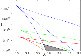
Figure 14: Comparision of $T$-$\lambda$ plot for three different flow geometries ($a=0.1$, $T$ in Kelvin). Constant height disc, quasi-spherical flow and flow in vertical hydrostatic equilibrium represented by blue dashed lines, green dotted lines and red solid lines respectively. The shaded region allows for multicritical solution in all flow configurations.

In figure 14, for $a=0.1$, we compare the parameter spaces for three different flow geometries. The common domain for which multiple critical points are formed for all three flow geometries is shown as a shaded region.

11 Classification of critical points for isothermal accretion

Using the same technique elaborated in section $4$, eigenvalues of the stability matrices for isothermal accretion can be computed for the three disc geometries.

11.1 Constant Height Flow

$${\Omega^{iso}_{CH}}^{2}={\mathcal{B}_{CH}^{iso}}{\mathcal{C}_{CH}^{iso}}$$ (89)

where,

$${{\cal B}_{CH}^{iso}} = \frac{{f_{c}^{{}^{\prime}}}}{f_{c}}\frac{a^{2}-1-(r_{c}-1)^{2}}{\Delta(r_{c}-1)}-\frac{{f_{c}^{{}^{\prime\prime}}}}{f_{c}}+\left(\frac{{f_{c}^{{}^{\prime}}}}{f_{c}}\right)^{2}$$ (90)

$${{\cal C}_{CH}^{iso}} = \frac{1}{u_{c}^{2}(1-u_{c}^{2})}$$ (91)

11.2 Conical Flow

$${\Omega^{iso}_{CF}}^{2}={\mathcal{B}_{CF}^{iso}}{\mathcal{C}_{CF}^{iso}}$$ (92)

where,

$${{\cal B}_{CF}^{iso}} = \frac{{f_{c}^{{}^{\prime}}}}{f_{c}(2r_{c}^{2}-3r_{c}+a^{2})}(-\frac{\Delta_{c}}{r_{c}}+\frac{r_{c}}{\Delta_{c}}(a^{2}-1-(r_{c}-1)^{2}))$$ (93)

$$-\frac{{f_{c}^{{}^{\prime\prime}}}}{f_{c}}+\left(\frac{{f_{c}^{{}^{\prime}}}}{f_{c}}\right)^{2}$$

$${{\cal C}_{CF}^{iso}} = \frac{1}{u_{c}^{2}(1-u_{c}^{2})}$$ (94)

11.3 Flow in hydrostatic equilibrium along the vertical direction

$${\Omega^{iso}_{VE}}^{2}={\mathcal{B}_{VE}^{iso}}{\mathcal{C}_{VE}^{iso}}-{\mathcal{A}_{VE}^{iso}}{\mathcal{D}_{VE}^{iso}}$$ (95)

$${{\cal A}_{VE}^{iso}} = \frac{{{c_{s}}_{c}}^{2}}{g_{2}}\left(\frac{(2\lambda^{2}v_{t}-a^{2}){f_{c}}^{{}^{\prime}}{g_{2}}^{{}^{\prime}}}{2g_{2}\sqrt{(1-u_{c}^{2})f_{c}}}-\delta_{3}\right)$$ (96)

$${{\cal B}_{VE}^{iso}} = {c_{s}}_{c}^{2}\left(\frac{2}{\Delta_{c}}-\frac{4}{r_{c}^{2}}-\frac{4(r_{c}-1)^{2}}{\Delta_{c}^{2}}-\frac{\delta_{4}}{g_{2}}\right.$$ (97)

$$\left.+\left(\frac{(2\lambda^{2}v_{t}-a^{2}){f_{c}}^{{}^{\prime}}}{2g_{2}\sqrt{(1-u_{c}^{2})f_{c}}}\right)^{2}\right)$$

$$-\frac{f_{c}^{{}^{\prime\prime}}}{f_{c}}+\left(\frac{f_{c}^{{}^{\prime}}}{f_{c}}\right)^{2}$$

$${{\cal C}_{VE}^{iso}} = \frac{u_{c}^{4}-2{c_{s}}_{c}^{2}u_{c}^{2}+{c_{s}}_{c}^{2}}{u_{c}^{4}(1-u_{c}^{2})^{2}}+\frac{{c_{s}}_{c}^{2}\delta_{1}}{g_{2}}-\frac{{c_{s}}_{c}^{2}{g_{2}^{{}^{\prime}}}^{2}}{g_{2}^{2}}$$ (98)

$${{\cal D}_{VE}^{iso}} = -{{\cal A}_{VE}^{iso}}$$ (99)

where,
$g_{2}=(\lambda v_{t})^{2}-v_{t}a^{2}+a^{2}$,
$\delta_{1}=\frac{2\lambda^{2}f}{(1-u_{c}^{2})^{3}}-\frac{3a^{2}}{4}\sqrt{\frac{f}{(1-u_{c}^{2})^{5}}}$,
$\delta_{3}=\frac{\lambda^{2}f^{\prime}}{(1-u_{c}^{2})^{2}}-\frac{a^{2}f^{\prime}}{4\sqrt{f(1-u_{c}^{2})^{3}}}$,
$\delta_{4}=\frac{\lambda^{2}f^{{}^{\prime\prime}}}{1-u_{c}^{2}}-\frac{a^{2}}{4\sqrt{1-u_{c}^{2}}}\frac{2ff^{{}^{\prime\prime}}-f^{\prime 2}}{f^{\frac{3}{2}}}$

12 Dependence of $\Omega^{2}$ on flow and spin parameters for isothermal accretion in various matter geometries

Figs. 15, 16 and 17 obtained by evaluating the analytical expressions for isothermal flow derived in the previous section at $r_{c}$ establish the same argument about multi-transonicity and nature of the critical points as presented in the corresponding section for polytropic flows. The numerical value of $\Omega^{2}$ assumes positive sign for the inner and outer saddle-type critical points and negative sign for the middle centre-type critical points.

Figure 15: Comparison of $\Omega^{2}$ vs. $\left[T,\lambda\right]$ of the inner and outer critical points for constant height flow (CH), quasi-spherical flow (CF) and flow in vertical hydrostatic equilibrium (VE) ($a=0.1$). Left and right panels depict $\Omega^{2}$ for inner and outer critical points respectively for CH, CF and VE from top to bottom in the respective order.

Figure 16: Comparison of $\Omega^{2}$ vs. $\left[T,\lambda\right]$ of the middle critical point for constant height flow (CH) (top left), quasi-spherical flow (CF) (top right) and flow in vertical hydrostatic equilibrium (VE) (bottom left)($a=0.1$).

In fig. 15, the variation of $\Omega^{2}$ for inner and outer critical points has been depicted over the entire physical domain of $\left[T,\lambda\right]$ for a given value of $a=0.1$. Positive values indicate critical points of saddle nature. Fig. 16 depicts the values of $\Omega^{2}$ for the middle critical points over the full accessible domain of $\left[T,\lambda\right]$ for the same value of $a$. Negative values indicate critical points which are centre-type. The same trend of comparision is observed between the absolute magnitudes of $\Omega^{2}$ for the saddle type critical points in the case of isothermal flow as well. $\Omega^{2}_{inner}>>\Omega^{2}_{outer}$ once again points towards a correlation between the absolute value of $\Omega^{2}$ and space-time curvature at the critical points. A comparision of the three different flow geometries reveals that for inner and middle critical points, $|\Omega^{2}|_{CH}>|\Omega^{2}|_{CF}>|\Omega^{2}|_{VE}$, whereas for the outer critical point $|\Omega^{2}|_{VE}>|\Omega^{2}|_{CF}>|\Omega^{2}|_{CH}$.

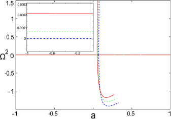
Figure 17: Comparison of $\Omega^{2}$ vs. $a$ for constant height flow (blue dashed lines), quasi-spherical flow (green dotted lines) and flow in vertical hydrostatic equilibrium (red solid lines)($T=10^{10}$ K, $\lambda=3.6$). Inset shows a magnified view of the common monotransonic region for the three flow geometries.

Fig. 17 is a similar plot as was obtained for polytropic flow depicting the bifurcation of $\Omega^{2}$ along black hole spin parameter $a$ for a given value of temperature and specific angular momentum ($T=10^{10}K,\lambda=3.6$). Monotransonic flow through a saddle type critical point is shown in the inset where $\Omega^{2}$ assumes a single positive value for all three flow geometries. The monotransonic flow then bifurcates into multi-transonic flow with a centre-type middle critical point (with negative value), a saddle-type inner critical point (with a larger positive value) and a saddle-type outer critical point (with a smaller positive value). Thus, a saddle-centre pair is generated at a definite value of $a$. The inner saddle gradually shifts closer to the event horizon acquiring higher values of $\Omega^{2}$ and finally one is left with a single saddle point through which physical monotransonic flow can occur. As in the case of polytropic flow, the value of parameter $a$ at which the bifurcation occurs is different for different flow geometries and that value is found to be minimum for discs in vertical hydrostatic equilibirum.

13 Shock-invariant quantities ($S_{h}$)

Applying the technique described in section 6.1, shock-invariant quantities ($S_{h}$) for all three isothermal flow geometries are obtained as under-

13.1 Constant height flow

$$S_{h}{|_{CH}^{iso}}=\left(\frac{u}{\sqrt{1-u^{2}}}\right)^{2{c_{s}^{2}}-1}(u^{2}\Delta+r^{2}{c_{s}^{2}}(1-u^{2}))$$ (100)

13.2 Conical flow

$$S_{h}{|_{CF}^{iso}}=\left(\frac{u}{\sqrt{1-u^{2}}}\right)^{2{c_{s}^{2}}-1}(u^{2}\Delta+r^{2}{c_{s}^{2}}(1-u^{2}))$$ (101)

13.3 Flow in hydrostatic equilibrium in the vertical direction

$$S_{h}{|_{VE}^{iso}}=u^{2{c_{s}^{2}}-1}(u^{2}\Delta+r^{2}{c_{s}^{2}}(1-u^{2}))$$ (102)

14 Shock parameter space for isothermal accretion

We now intend to see which region of the $T-\lambda$ parameter space allows shock formation. For a fixed of $a=0.1$, we check validity of the Rankine Hugoniot condition for every value of $\left[T,\lambda\right]$ for which the accretion flow possesses three critical points. This means the shock-invariant quantity is calculated for every $\left[T,\lambda\right]$ for which the multitransonic accretion is possible, and it is observed that only for some subset of such $\left[T,\lambda\right]$, the shock-invariant quantities calculated along the solution passing through the outer and the inner sonic points become equal at a particular radial distance, i.e., at the shock location. We then plot the corresponding $\left[T,\lambda\right]_{\rm{shock}}$ for various geometric configurations of matter.

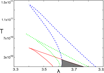
Figure 18: Comparision of $T$-$\lambda$ plot of allowed shocked multitransonic accretion solutions for three different flow geometries ($a=0.1$, $T$ in Kelvin). Constant height disc, quasi-spherical flow and flow in vertical hydrostatic equilibrium represented by blue dashed lines, green dotted lines and red solid lines respectively. Shaded region depicts the overlapping domain of shock formation in all the three geometries.

In fig. 18 we plot the subsets of the $T$-$\lambda$ spaces for three different flow geometries at a fixed $a$ ($=0.1$), for which, value of the shock-invariant quantities $S_{h}$, when evaluated along the flow branches through inner and outer critical points, become equal at particular value(s) of $r$. This value of radial distance $r_{sh}$ is the location of shock. The shaded region depicts overlap of shock-forming $\left[T,\lambda\right]$ parameter set of the three disc configurations for a given $a$.

Once the common region for shock formation is obtained, we investigate the variation of shock location ($r_{sh}$), shock strength ($M_{+}/M_{-}$), compression ratio ($\rho_{-}/\rho_{+}$), pressure ratio ($P_{-}/P_{+}$) and quasi-specific energy dissipation ratio ($\xi_{+}/\xi_{-}$) ($+$ and $-$ have the same meanings as defined for polytropic accretion) on the black hole spin parameter $a$, also comparing the trends of variation for various disc geometries.

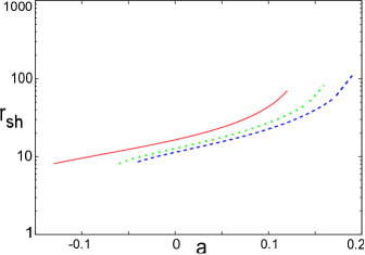
Figure 19: Shock location ($r_{sh}$) vs. $a$ plot ($T=10^{10}K,\lambda=3.75$) for constant height disc (dashed blue line), quasi-spherical disc (dotted green line) and flow in hydrostatic equilibrium (solid red line).

Fig. 19 shows how the shock location ($r_{sh}$) varies with spin parameter $a$. The bulk ion temperature has been fixed at $10^{10}$ K and the value of $\lambda$ has been selected accordingly ($=3.75$) from the region of shock overlap observed in fig. 18 so that the available range of $a$ is maximum. The same set of $\left[T,\lambda\right]$ has been used in all subsequent shock related plots. As already argued in the corresponding section for polytropic flow, growth in strength of the effective centrifugal barrier due to increase in the difference between $\lambda$ and $a$ explains the formation of shock farther away from the gravitating source as the value of black hole spin is increased while keeping the value of specific angular momentum fixed. Again, for a particular value of $a$, it is observed that $r_{sh}(VE)>r_{sh}(CF)>r_{sh}(CH)$, which indicates that even in the case of isothermal flow, an accretion disc in vertical hydrostatic equilibrium is exposed to maximum resistance for a given centrifugal barrier.

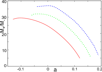
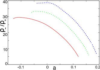
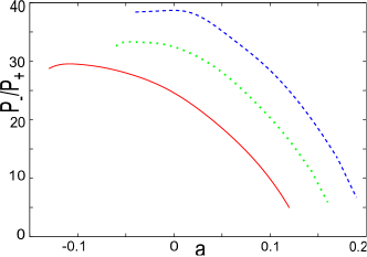
Figure 20: Variation of shock strength ($M_{+}/M_{-}$), compression ratio ($\rho_{-}/\rho_{+}$) and pressure ratio ($P_{-}/P_{+}$) with black hole spin parameter $a$ ($E=10^{10}K,\lambda=3.75$) for constant height flow (dashed blue lines), quasi-spherical flow (dotted green lines) and flow in hydrostatic equilibrium (solid red lines). Subscripts ‘+’ and ‘-’ represent pre and post shock quantities respectively.

Figure (20) on comparing with fig.(11) establishes the fact that irrespective of whether the flow is polytropic or isothermal, a gradual increase in black hole spin for a specific flow angular momentum shifts the shock location outwards by boosting the effective centrifugal barrier. A shock formed far away from the event horizon is weaker in strength owing to the eventual flattening of space-time. Moreover in both polytropic and isothermal cases, for a given $\left[a,\lambda\right]$, the strongest shocks are formed in constant height discs whereas discs in hydrostatic vertical equilibrium exhibit the weakest shocks. The same trend is consistently observed for all the relevant ratios across the discontinuity.

15 Powering the flares through the energy dissipated at the shock

For the isothermal accretion onto a rotating black hole considered in the present work, we concentrate on dissipative shocks. Unlike the standing Ranking-Hugoniot type energy-preserving shocks studied for the polytropic flow, a substantial amount of energy is dissipated at the shock location to maintain the temperature invariance of the isothermal flow. As a consequence, the flow thickness does not change abruptly at the shock location, and handling the pressure balance equation across the shock becomes more convenient as compared to that for the polytropic accretion. The amount of energy dissipated at the shock might make an isothermal shock to appear ‘bright’, since for inviscid, dissipationless flow as considered in our work, accretion remains grossly radiatively inefficient throughout.
The type of low angular momentum inviscid flow we consider in the present work, is believed to be ideal to mimic the accretion environment of our galactic centre black hole (Moscibrodzka et al. (2006)). Sudden substantial energy dissipation from the shock surface may thus be conjectured to feed the X-ray and IR flares emanating from our galactic centre black hole (Baganoff et al. (2001), Genzel et al. (2003), Marrone et al. (2008), Czerny et al. (2010), Wang et al. (2013), Ponti et al. (2015), Karssen et al. (2017), Mossoux and Grosso (2017), Yuan et al. (2018)).
In our formalism, the ratios of the quasi-specific energies corresponding to the pre-shock and post-shock flows is assumed to be a measure of the amount of the dissipated energy at the shock surface. In fig. 21, we plot such ratios for various ranges of the black hole spins (the Kerr parameter ‘$a$’) for three different types of the geometrical thicknesses of the flow as considered in our present work. There are four panels in the figure, each plane corresponding to a certain range of values of the black hole spin angular momentum. As already discussed, for a fixed value of $\left[\mathcal{E},\lambda,\gamma\right]$ or $\left[T,\lambda\right]$, shock formation over a continuous range of ‘$a$’ spanning the entire domain of the Kerr parameter $-1>a>1$, is allowed neither for polytropic nor isothermal accretion. Four different panels in the figure are thus characterised by four different sets of $\left[T,\lambda\right]$ as mentioned in the figure caption. The following interesting features are observed:

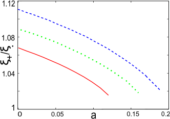
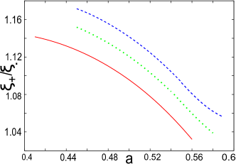
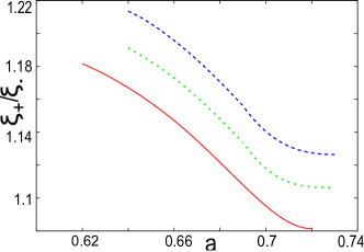
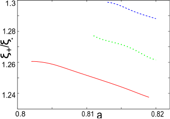
Figure 21: Variation of quasi-specific energy ratio ($\xi_{+}/\xi_{-}$) with black hole spin parameter $a$ ($T=10^{10}$ K). In order to obtain multicritical domains with shock over four different ranges of $a$, four different values of $\lambda$ have been set at the given $T$, i.e. $\lambda=3.75$ (upper left), $\lambda=3.25$ (upper right), $\lambda=3.0$ (lower left), $\lambda=2.7$ (lower right). Constant height flow, quasi-spherical flow and flow in hydrostatic equilibrium have been represented by dashed blue lines, dotted green lines and solid red lines. Subscripts ‘+’ and ‘-’ represent pre and post shock quantities respectively.

Depending on the initial conditions, substantial amount of energy gets liberated from the shock surface. Sometimes even as high as $30\%$ of the rest mass may be converted into radiated energy, which is a huge amount. Hence the shock-generated dissipated energy can, in principle, be considered as a good candidate to explain the source of energy dumped into the flare.
The length scale on the disc from which the flare may be generated actually matches with the shock location. Such ‘flare generating’ length scales obtained in our theoretical calculations are thus, in good agreement with the observational works (Karssen et al. (2017)).
What we actually observe is that the amount of dissipated energy anti-correlates with the shock location, which is perhaps intuitively obvious because closer the shock forms to the horizon, greater is the available gravitational energy to be converted into dissipated radiation.
Following the same line of argument, the amount of dissipated energy anti-correlates with the flow angular momentum. Lower is the angular momentum of the flow, the centrifugal pressure supported region forms closer to the boundary. Such regions slow down the flow and break the flow behind it, and hence the shock forms. The locations of such region are thus markers anticipating from which region of the disc, the flare may be generated.
It is imperative to study the influence of the black hole spin in determining the amount of energy liberated at the shock. What we find here is that for the prograde flow, such amount anti- correlates with the black hole spin. Thus, for a given flow angular momentum, slowly rotating black holes produce the strongest flares. Hence, for a given value of $\left[T,\lambda\right]$, if shocked multitransonic accretion solutions exist over a positive span of $a$ including $a=0$, then flares originating from the vicinity of the Schwarzschild hole would consequently contain the maximum amount of energy. Hence, unlike the Blandford-Znajek mechanism (Blandford and Znajek (1977), Das and Czerny (2012), O’ Riordan et al. (2016), Czerny and You (2016), Bambi (2017)), the amount of energy transferred to a flare is not extracted at the expense of black hole spin.
Certain works based on the observational results argue that there is no obvious correlation between the black hole spin and the jet power (Fender et al. (2010), Broderick and Fender (2011) and references therein). Our present finding is in accordance with such arguments.
In this connection, however, it is to be noted that BZ mechanism is usually associated with the electromagnetic energy extractions, whereas energy liberation at the shock is associated with the hydrodynamic flow. Hence no direct comparision can perhaps be made between the Blandford Znajek process and the process considered in our work.

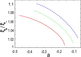
Figure 22: Variation of quasi-specific energy ratio ($\xi_{+}/\xi_{-}$) with black hole spin parameter $a$ ($T=10^{10}$ K, $\lambda=4.0$) for retrograde flow. Constant height flow, quasi-spherical flow and flow in hydrostatic equilibrium have been represented by dashed blue lines, dotted green lines and solid red lines. Subscripts ‘+’ and ‘-’ represent pre and post shock quantities respectively.

In recent years, the study of retrograde flow close to the Kerr holes are also of profound interest (Garofalo (2013), Mikhailov et al. (2018) and references therein). We thus study the spin dependence of the amount of energy dissipation at the shock. The result is shown in fig. 22. Here we observe that the amount of dissipated energy is more for faster counter-rotating holes. For retrograde flow, the negative Kerr parameter essentially reduces the overall measure of the angular momentum of the flow and the effective angular momentum may probably be thought of as $\lambda_{eff}=\lambda-a$, which explains such finding.
It is also observed that the amount of shock dissipated energy is also influenced by the geometric configuration of the flow. We find that axially symmetric flow with constant thickness produces largest amount of liberated energy at the shock, whereas the flow in hydrostatic equilibrium along the vertical direction produces the smallest amount. The conical wedge shaped flow contributes at a rate which is intermediate to the rates for the constant height disc and the disc in vertical equilibrium. This feature remains unaltered for the prograde as well as the retrograde flows.

16 Quasi-terminal values

16.1 Dependence of $\left[M,\rho,P\right]_{r_{\delta}}$ on $a$ for shocked isothermal accretion

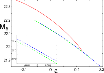
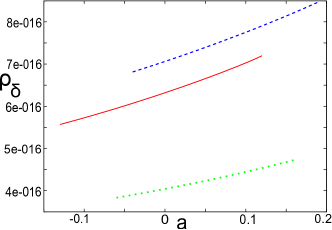
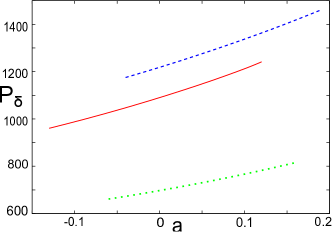
Figure 23: Variation of quasi-terminal values of Mach number ($M_{\delta}$), density ($\rho_{\delta}$) and pressure ($P_{\delta}$) with $a$ ($T=10^{10}K,\lambda=3.75$) for constant height flow (dashed blue lines), quasi-spherical flow (dotted green lines) and flow in hydrostatic equilibrium (solid red lines). Density and pressure are in CGS units of $g$ $cm^{-3}$ and $dyne$ $cm^{-2}$ respectively and temperature is in absolute units of Kelvin.

Variation of the quasi-terminal values of Mach number ($M_{\delta}$), density ($\rho_{\delta}$) and pressure ($P_{\delta}$) with spin parameter $a$ has been shown in fig.(23) for a given $T$ ($=10^{10}$) and $\lambda$ ($=3.75$). It is observed that although the variations are similar in nature to those for polytropic flow, but even in this case, limitations in the availibility and overlap of a broad range of spin for shocked multitransonic accretion for all geometric models, make it impossible to comment on the global trend with which such quantities vary in accordance to black hole spin or the disc configuration. Hence, we try to resolve this issue in the next subsection by looking at the case of monotransonic isothermal accretion.

16.2 Dependence of $\left[M,\rho,P\right]_{r_{\delta}}$ on $a$ for monotransonic isothermal accretion

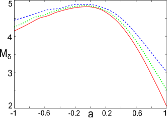
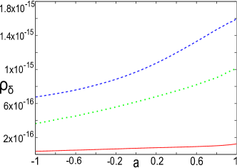
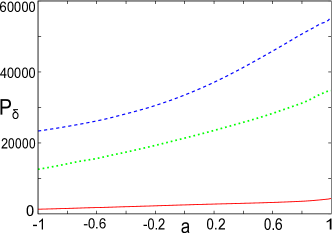
Figure 24: Variation of quasi-terminal values of Mach number ($M_{\delta}$), density ($\rho_{\delta}$) and pressure ($P_{\delta}$) with $a$ ($T=2\times 10^{11}K,\lambda=2.0$) for monotransonic accretion in constant height flow (dashed blue lines), quasi-spherical flow (dotted green lines) and flow in hydrostatic equilibrium (solid red lines). Density and pressure are in CGS units of $g$ $cm^{-3}$ and $dyne$ $cm^{-2}$ respectively and temperature is in absolute units of Kelvin.

Fig.(24) depicts how quasi-terminal values of Mach number, density and pressure of monotransonic isothermal flow depend on the Kerr parameter. Hot flows with low angular momentum exhibit stationary accretion solutions spanning the full domain of black hole spin. It is observed that the general spin dependent behaviour of the corresponding physical quantities for three different flow geometries is quite well behaved in case of isothermal accretion, as opposed to the polytropic case. However, the previously stated intrinsic limitations in the possibility of observing variations over complete range of spin still exist for multitransonic flows. It is clear from fig.(24) that quasi-terminal values possess common global trends of variation over $a$ for all three geometric configurations. The important observation in this context is the existence of asymmetry in variation of the related quantities between prograde and retrograde spin of the black hole. As mentioned in the case of polytropic accretion, such asymmetry is an extremely significant finding for the observation of black hole spin related effects.

17 Concluding Remarks

Computation of the quasi-terminal values helps us to understand the nature of spectra for which photons have emanated from a close proximity of the horizon. Hence, variation of the quasi-terminal values may be useful to understand how the black hole spin influences the configuration of the image of the black hole shadow. The present work puts forth two important findings which are worth mentioning in this context. Firstly, the spin dependence of quasi-terminal values has been studied for different geometrical configurations of matter. Secondly, we have found that (see, e.g. figs.(13) and (24)) the prograde and the retrograde flows are distinctly marked by asymmetric distributions of relevant quasi-terminal values over the entire theoretical range of Kerr parameter. This indicates that the constructed image of shadow will be different for the co- and counter rotating flows. We also observe that the physical quantities responsible to construct the black hole spectra (velocity, density, pressure, temperature (for polytropic accretion) and quasi-specific energy (for isothermal accretion) of the flow) change abruptly at the shock location. This indicates that the discontinuous changes in the physical quantities should be manifested as a break in the corresponding spectral index, and will also show up during the procedure of black hole shadow imaging. Our work is thus expected to predict how the shape of the image of the shadow might be governed by the dynamical and thermodynamic properties of the accretion flow along with the spin of black hole. Through the construction of such image (work in progress), we will not only be able to provide a possible methodology (atleast at a qualitative level) for the observational signature of the black hole spin, but such images will also possibly shed light on the difference between the prograde and retrograde flows from an observational point of view. We have analysed general relativistic accretion of both polytropic and isothermal fluids in the Kerr metric to study the effects of matter geometry and black hole spin parameter on multitransonic shocked accretion flow.

References

- Abramowicz and Zurek [1981] M. A. Abramowicz and W. H. Zurek. ApJ, 246:314, 1981.
- Abramowicz et al. [1997] M. A. Abramowicz, A. Lanza, and M. J. Percival. ApJ, 479:179, 1997.
- Baganoff et al. [2001] F. K. Baganoff, M. W. Bautz, W. N. Brandt, G. Chartas, E. D. Feigelson, G. P. Garmire, Y. Maeda, M. Morris, G. R. Ricker, L. K. Townsley, and F. Walter. Rapid X-ray flaring from the direction of the supermassive black hole at the Galactic Centre. Nature, 413:45–48, September 2001. doi: 10.1038/35092510.
- Bambi [2017] Cosimo Bambi. Testing black hole candidates with electromagnetic radiation. Reviews of Modern Physics, 89:025001, April 2017. doi: 10.1103/RevModPhys.89.025001.
- Bilić et al. [2014] N. Bilić, A. Choudhary, T. K. Das, and S. Nag. Classical & Quantum Gravity, 31:35002, 2014.
- Blaes [1987] O. Blaes. MNRAS, 227:975, 1987.
- Blandford and Znajek [1977] R. D. Blandford and R. L. Znajek. Electromagnetic extraction of energy from Kerr black holes. MNRAS, 179:433–456, May 1977. doi: 10.1093/mnras/179.3.433.
- Bollimpalli et al. [2017] D. A. Bollimpalli, S. Bhattacharya, and T. K. Das. New Astronomy, 51:153, 2017.
- Brenneman [2013] L. Brenneman. Springer Briefs in Astronomy, pages 978–1, 2013.
- Broderick and Fender [2011] J. W. Broderick and R. P. Fender. Is there really a dichotomy in active galactic nucleus jet power? MNRAS, 417:184–197, October 2011. doi: 10.1111/j.1365-2966.2011.19060.x.
- Buliga et al. [2011] S. D. Buliga, V. I. Globina, Y. N. Gnedin, T. M. Natsvlishvili, M. Y. Pitrovich, and N. A. Shakht. Astrophysics, 54(4):548, 2011.
- Czerny and You [2016] B. Czerny and B. You. Accretion in active galactic nuclei and disk-jet coupling. Astronomische Nachrichten, 337:73, February 2016. doi: 10.1002/asna.201512268.
- Czerny et al. [2007] B. Czerny, M. Mościbrodzka, D. Proga, T. K. Das, and A. Siemiginowska. Low angular momentum accretion flow model of Sgr A* activity. In S. Hledík and Z. Stuchlík, editors, Proceedings of RAGtime 8/9: Workshops on Black Holes and Neutron Stars, pages 35–44, December 2007.
- Czerny et al. [2010] B. Czerny, P. Lachowicz, M. Dovčiak, V. Karas, T. Pecháček, and T. K. Das. The model constraints from the observed trends for the quasi-periodic oscillation in RE J1034+396. Astronomy & Astrophysics, 524:A26, December 2010. doi: 10.1051/0004-6361/200913724.
- Daly [2011] Ruth. A. Daly. Estimates of black hole spin properties of 55 sources. MNRAS, 414:1253–1262, June 2011. doi: 10.1111/j.1365-2966.2011.18452.x.
- Das et al. [2015] T. K. Das, S. Nag, S. Hegde, S. Bhattacharya, I. Maity, B. Czerny, P. Barai, P. J. Wiita, V. Karas, and T. Naskar. New Astronomy, 37:81, 2015.
- Das and Czerny [2012] Tapas K. Das and B. Czerny. On the efficiency of the Blandford-Znajek mechanism for low angular momentum relativistic accretion. MNRAS, 421:L24–L28, March 2012. doi: 10.1111/j.1745-3933.2011.01199.x.
- Dauser et al. [2010] T. Dauser, J. Wilms, C. S. Reynolds, and L. W. Brenneman. MNRAS, 409:1534, 2010.
- Dotti et al. [2013] M. Dotti, M. Colpi, S. Pallini, A. Perego, and M. Volonteri. ApJ, 762(2):10, 2013.
- Esin et al. [1997] A. A. Esin, J. E. McClintock, and R. Narayan. The Astrophysical Journal, 489:865–889, 1997.
- Fabian et al. [2014] A. C. Fabian, M. L. Parker, D. R. Wilkins, J. M. Miller, E. Kara, C. S. Reynolds, and T. Dauser. MNRAS, 439:2307, 2014.
- Falcke et al. [2000] H. Falcke, F. Melia, and E. Agol. American Institute of Physics Conference Series, 522:317–320, 2000.
- Fender et al. [2010] R. P. Fender, E. Gallo, and D. Russell. No evidence for black hole spin powering of jets in X-ray binaries. MNRAS, 406:1425–1434, August 2010. doi: 10.1111/j.1365-2966.2010.16754.x.
- Garofalo [2013] David Garofalo. Retrograde versus Prograde Models of Accreting Black Holes. Advances in Astronomy, 2013:213105, January 2013. doi: 10.1155/2013/213105.
- Genzel et al. [2003] R. Genzel, R. Schödel, T. Ott, A. Eckart, T. Alexander, F. Lacombe, D. Rouan, and B. Aschenbach. Near-infrared flares from accreting gas around the supermassive black hole at the Galactic Centre. Nature, 425:934–937, October 2003. doi: 10.1038/nature02065.
- Goswami et al. [2007] S. Goswami, S. N. Khan, A. K. Ray, and T. K. Das. MNRAS, 378:1407, 2007.
- Healy et al. [2014] J. Healy, C. Lousto, and Y. Zlochower. arXiv:1406.7295 [gr-qc], 2014.
- Hioki and Maeda [2009] Kenta Hioki and Kei-Ichi Maeda. Measurement of the Kerr spin parameter by observation of a compact object’s shadow. Physical Review D, 80:024042, July 2009. doi: 10.1103/PhysRevD.80.024042.
- Huang et al. [2007] L. Huang, M. Cai, Z. Q. Shen, and F. Yuan. MNRAS, 379:833–840, 2007.
- Jiang et al. [2014] J. Jiang, C. Bambi, and J.F. Steiner. arXiv:1406.5677 [gr-qc], 2014.
- Jordan and Smith [1999] D. W. Jordan and P. Smith. Nonlinear Ordinary Differential Equations. Oxford University Press, Oxford, 1999.
- Karssen et al. [2017] G. D. Karssen, M. Bursa, A. Eckart, M. Valencia-S, M. Dovčiak, V. Karas, and J. Horák. Bright X-ray flares from Sgr A*. MNRAS, 472:4422–4433, December 2017. doi: 10.1093/mnras/stx2312.
- Kato et al. [2010] Y. Kato, M. Miyoshi, R. Takahashi, H. Negoro, and R. Matsumoto. MNRAS, 403:L74, 2010.
- Marrone et al. [2008] D. P. Marrone, F. K. Baganoff, M. R. Morris, J. M. Moran, A. M. Ghez, S. D. Hornstein, C. D. Dowell, D. J. Muñoz, M. W. Bautz, G. R. Ricker, W. N. Brandt, G. P. Garmire, J. R. Lu, K. Matthews, J. H. Zhao, R. Rao, and G. C. Bower. An X-Ray, Infrared, and Submillimeter Flare of Sagittarius A*. Astrophysical Journal, 682:373–383, July 2008. doi: 10.1086/588806.
- Martínez-Sansigre and Rawlings [2011] Alejo Martínez-Sansigre and Steve Rawlings. Observational constraints on the spin of the most massive black holes from radio observations. MNRAS, 414:1937–1964, July 2011. doi: 10.1111/j.1365-2966.2011.18512.x.
- McClintock et al. [2011] J. E. McClintock, R. Narayan, S. W. Davis, L. Gou, A. Kulkarni, J. A. Orosz, R. F. Penna, R. A. Remillard, and J. F. Steiner. Classical and Quantum Gravity, 28(11):114009, 2011.
- McKinney et al. [2013] J. C. McKinney, A. Tchekhovskoy, and R. D. Blandford. Science, 339:49, 2013.
- Mikhailov et al. [2018] A. G. Mikhailov, M. Yu Piotrovich, Yu N. Gnedin, T. M. Natsvlishvili, and S. D. Buliga. Criteria for retrograde rotation of accreting black holes. MNRAS, 476:4872–4876, June 2018. doi: 10.1093/mnras/sty643.
- Miller et al. [2009] J. M. Miller, C. S. Reynolds, A. C. Fabian, G. Miniutti, and L. C. Gallo. ApJ, 697:900–912, 2009.
- Moscibrodzka et al. [2006] M. Moscibrodzka, T. K. Das, and B. Czerny. MNRAS, 370:219, 2006.
- Mossoux and Grosso [2017] Enmanuelle Mossoux and Nicolas Grosso. Sixteen years of X-ray monitoring of Sagittarius A*: Evidence for a decay of the faint flaring rate from 2013 August, 13 months before a rise in the bright flaring rate. Astronomy & Astrophysics, 604:A85, August 2017. doi: 10.1051/0004-6361/201629778.
- Nemmen and Tchekhovskoy [2014] R. Nemmen and A. Tchekhovskoy. arXiv:1406.7420 [astro-ph.HE], 2014.
- Nixon et al. [2011] C. J. Nixon, P. J. Cossins, A. R. King, and J. E. Pringle. MNRAS, 412:1591, 2011.
- O’ Riordan et al. [2016] Michael O’ Riordan, Asaf Pe’er, and Jonathan C. McKinney. Effects of Spin on High-energy Radiation from Accreting Black Holes. Astrophysical Journal, 831:62, November 2016. doi: 10.3847/0004-637X/831/1/62.
- Paczyński and Wiita [1980] B. Paczyński and P. J. Wiita. A & A, 88:23, 1980.
- Ponti et al. [2015] G. Ponti, B. De Marco, M. R. Morris, A. Merloni, T. Muñoz-Darias, M. Clavel, D. Haggard, S. Zhang, K. Nandra, S. Gillessen, K. Mori, J. Neilsen, N. Rea, N. Degenaar, R. Terrier, and A. Goldwurm. Fifteen years of XMM-Newton and Chandra monitoring of Sgr A¡SUP¿?¡/SUP¿: evidence for a recent increase in the bright flaring rate. MNRAS, 454:1525–1544, December 2015. doi: 10.1093/mnras/stv1537.
- Reynolds et al. [2012] C. S. Reynolds, L. W. Brenneman, A. M. Lohfink, M. L. Trippe, J. M. Miller, R. C. Reis, M. A. Nowak, and A. C. Fabian. AIP Conference Proceedings, 1427:157–164, 2012.
- Sesana et al. [2014] A. Sesana, E. Barausse, M. Dotti, and E. M. Rossi. arXiv:1402.7088 [astro-ph.CO], 2014.
- Straub et al. [2012] O. Straub, F. H. Vincent, M. A. Abramowicz, E. Gourgoulhon, and T. Paumard. Astronomy & Astrophysics, 543:A83, 2012.
- Strogatz [2001] S. H. Strogatz. Nonlinear Dynamics And Chaos: With Applications To Physics, Biology, Chemistry, And Engineering. Westview Press, 2001.
- Takahashi [2004] R. Takahashi. IAU Symposium Proccedings, 222:115–116, 2004.
- Tarafdar and Das [2018] Pratik Tarafdar and Tapas K. Das. Influence of matter geometry on shocked flows-I: Accretion in the Schwarzschild metric. New Astronomy, 62:1–14, July 2018. doi: 10.1016/j.newast.2017.12.007.
- Tchekhovskoy and McKinney [2012] A. Tchekhovskoy and J. C. McKinney. MNRAS, 423(1):L55, 2012.
- Tchekhovskoy et al. [2010] A. Tchekhovskoy, R. Narayan, and J. C. McKinney. ApJ, 711:50, 2010.
- Wang et al. [2013] Q. D. Wang, M. A. Nowak, S. B. Markoff, F. K. Baganoff, S. Nayakshin, F. Yuan, J. Cuadra, J. Davis, J. Dexter, A. C. Fabian, N. Grosso, D. Haggard, J. Houck, L. Ji, Z. Li, J. Neilsen, D. Porquet, F. Ripple, and R. V. Shcherbakov. Dissecting X-ray-Emitting Gas Around the Center of Our Galaxy. Science, 341:981–983, August 2013. doi: 10.1126/science.1240755.
- Yuan et al. [2018] Qiang Yuan, Q. Daniel Wang, Siming Liu, and Kinwah Wu. A systematic Chandra study of Sgr A*: II. X-ray flare statistics. MNRAS, 473:306–316, January 2018. doi: 10.1093/mnras/stx2408.
- Zakharov et al. [2012] A. F. Zakharov, F. D. Paolis, G. Ingrosso, and A. A. Nucita. New Astronomy Reviews, 56:64–73, 2012.
- Ziolkowski [2010] J. Ziolkowski. Memorie della Societ’A Astronomica Italiana, 81:294, 2010.