Independent Noise Synchronizing Networks of Oscillator Networks

Abstract

Oscillators coupled in a network can synchronize with each other to yield a coherent population rhythm. If multiple such networks are coupled together, the question arises whether these rhythms will synchronize. We investigate the impact of noise on this synchronization for strong inhibitory pulse-coupling and find that increasing the noise can synchronize the population rhythms, even if the noisy inputs to different oscillators are completely uncorrelated. Reducing the system to a phenomenological iterated map we show that this synchronization of the rhythms arises from the noise-induced phase heterogeneity of the oscillators. The synchronization of population rhythms is expected to be particularly relevant for brain rhythms.

The synchronization of coupled oscillators has been studied extensively DoeBul14 ; RodKur16 . Classical examples of technologically important synchronization include arrays of microwave oscillators YoCo91 or lasers BrJo05 , networks of Josephson junctions WiCo96 and optomechanical oscillators ZhaLip12 . Biological systems in which synchronization plays a central functional role include pacemaker cells in the heart MiMa87 and in the suprachiasmatic nucleus of the brain, which controls the circadian rhythm LiWe97 . Various types of rhythmic, coherent activity of large ensembles of neurons have been observed in many brain regions Wa10 . What functional role they may play in the information processing performed by the brain is still under debate BuzSch15 ; Fri15 .

Noise typically counteracts the synchronization of oscillators. Only if the noise driving different oscillators is sufficiently correlated does an increase in the noise level lead to synchronization Pi84 ; ZhKu02 ; TeTa04 . This noise-induced synchronization does not require any coupling between the oscillators; it essentially reflects the transfer of noise correlations from the input to the output ShJo08 ; AboErm11 .

If the oscillators in a network are sufficiently strongly synchronized due to their coupling, the whole network of oscillators can be thought of as a single composite network oscillator undergoing rhythmic population activity. If multiple such networks, each supporting its own rhythm, are coupled together, the question arises under what conditions such population rhythms phase-lock or synchronize and how that synchronization is affected by noise. Does the composite nature of the network oscillators introduce aspects that are not found in coupled individual oscillators?

Brain rhythms constitute an important class of population dynamics of oscillator networks. Among these the widely observed $\gamma$-rhythm (30-100 Hz) has been studied particularly extensively BuzWan12 . It typically arises either from the inhibitory interaction among interneurons (‘ING-rhythm’) or the reciprocal interaction between excitatory and inhibitory neurons (‘PING-rhythm’) WhTr00 ; BrWa03 ; BoKo03 ; TiSe09 . Importantly, $\gamma$-rhythms can arise simultaneously in different brain areas and rhythms in different areas may or may not be coherent with each other BosFri12 . Even within a single brain area they can differ in frequency and phase NeHa03 ; KaLa10 . Experiments show that the degree of coherence of $\gamma$-rhythms in different brain areas can depend on the attentional state of the animal GrGo09 ; BosFri12 ; RobDeW13 and it has been suggested that this coherence may play an important role in the communication between these areas Fri15 .

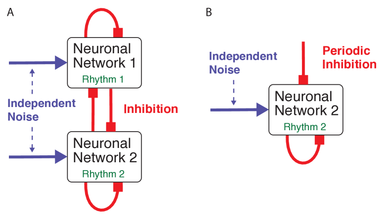
Figure 1: A) Two coupled inhibitory networks exhibiting separate $\gamma$-rhythms driven by independent noise. B) Simplified system with network 1 replaced by time-periodic inhibition.

This paper is motivated by i) the wide-spread occurence of modular networks RaSo02 ; BuSp09 , which can be considered as coupled networks, ii) the observation of coherence of $\gamma$-rhythms across different brain areas BosFri12 , and iii) the appearance of multiple, different $\gamma$-rhythms in a single brain area NeHa03 ; KaLa10 that is likely to exhibit modular structure as a result of learning via structural plasticity ChoRie12 ; SaiLle16 . To investigate the role noise can play in the interaction of such rhythms we consider coupled neuronal networks that each support their own $\gamma$-rhythm and that interact via inhibitory pulses (Fig.1A). The synchronization of modular networks has been studied using the master stability function approach PaLa06 ; SoOt07 and for diffusively coupled phase oscillators within the framework of the Kuramoto model OhRh05 ; ArDi08 ; GuWa08 , which arises in the weak-coupling limit. By contrast, we investigate a strong-coupling regime in which the inhibitory pulses can prevent individual neurons from firing.

As a main result we find that different $\gamma$-rhythms can become synchronized by noise even if that noise consists of independent Poisson spike trains and is therefore completely uncorrelated between different neurons and networks. This is in contrast to the well-studied case of noise-induced synchronization for which noise correlations are essential Pi84 ; TeTa04 . By reducing the coherent dynamics of the two networks to a minimal iterated map we show that the noise-induced phase heterogeneity allows the faster network to suppress the spiking of a fraction of the neurons in the slower network. This increases the frequency of the slower network and allows it to synchronize with the faster network. The synchronization leads to a more consistent phase relationship in the output of the two networks. We illustrate that this can increase the learning speed of downstream neurons that read the network output via synapses exhibiting spike-timing-dependent plasticity.

We consider two coupled networks of $N/2$ integrate-fire neurons each that receive $C_{1}=\epsilon_{1}N$ random inhibitory connections from their own network and $C_{2}=\epsilon_{2}N$ random inhibitory connections from the other network. Thus, all neurons have the same in-degree. In addition, each neuron receives noisy external excitatory inputs $I_{i}^{(ext)}(t)$ . The depolarization $V_{i}(t)$ of neuron $i$, $i=1,\dots,N$, is given by

$$\tau\dot{V}_{i}=V_{rest}-V_{i}+RI_{i}^{(syn)}(t)+RI_{i}^{(ext)}(t),$$ (1)

where $I_{i}^{(syn)}(t)$ denotes the total synaptic current from within the networks, $\tau$ the membrane time constant, and $R$ the membrane resistance. When $V_{i}(t)$ reaches the firing threshold $V_{\theta}$, a spike is triggered and the voltage is reset to the reset voltage $V_{r}$.

The synaptic currents are modeled as the difference of two exponentials, triggered by spikes of the presynaptic neuron $j$ at times $t_{j}^{(k)}$,

$$I_{i}^{(syn)}=\frac{g_{syn}}{R}\left(A_{i}^{(2)}-A_{i}^{(1)}\right)\left(V^{(rev)}-V\right),$$

with

$$\dot{A}_{i}^{(1,2)}=-\frac{A_{i}^{(1,2)}}{\tau_{1,2}}+\sum_{j=1}^{N}\sum_{k}W_{ij}\,\delta\left(t-t_{j}^{(k)}-\tau_{d}\right).$$ (2)

Here $V_{i}^{(rev)}$ denotes the reversal potential, $g_{syn}$ the dimensionless synaptic strength, and $\tau_{d}$ the synaptic delay. The connectivity matrix is denoted by $\mathbf{W}$ with its non-zero elements given by $W_{ij}=1$ if neuron$i$ and $j$ belong to the same network while $W_{ij}=\gamma_{0}$ if they belong to different networks.

The external input of each neuron $i$ is modeled as an independent Poisson-train of $\delta$-spikes at times $t_{ik}^{(ext)}$,

$$I_{i}^{(ext)}(t)=\frac{1}{R}\Delta V_{i}\sum_{k}\delta(t-t_{ik}^{(ext)}).$$ (3)

Thus, the noisy external inputs to different neurons are uncorrelated. The dimensionless input strengths $\Delta v_{i}\equiv\Delta V_{i}/(V_{\theta}-V_{r})$ are equal for all neurons within a network, but may differ between the two networks: $\Delta v_{i}=\Delta v^{(l)}$ for neurons in network $l$ with $\Delta v^{(2)}=\rho\Delta v^{(1)}$. Instead of the spike rates $\lambda$ and the strengths $\Delta v^{(1)}$ we use the mean input $\mu=\lambda\Delta v^{(1)}$and its variance $\sigma^{2}=\lambda(\Delta v^{(1)})^{2}$ as independent parameters.

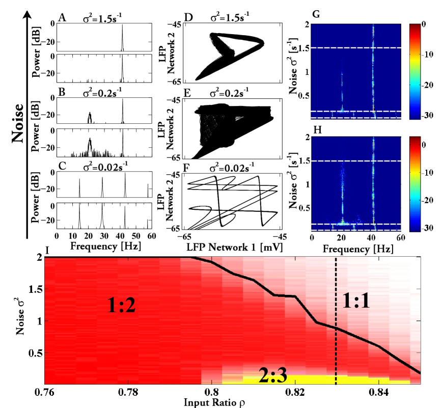
Figure 2: Independent noise synchronizes population activity of two coupled networks (cf. Fig.1A). Fourier spectra of the two networks (A,C,E correspond to the dashed lines in G,H) and the corresponding attractors (B,D,F) for $\rho=0.83$. Phase diagram showing transitions between different phase-locked and synchronized states as a function of noise. Color hue indicates frequency ratio, intensity the logarithmic power of the dominant Fourier mode (I). Parameters: $N=1,000$, $\epsilon_{1}=0.28$, $\epsilon_{2}=0.12$, $\tau=20\mbox{ms}$, $\tau_{1}=4.82\mbox{ms}$, $\tau_{2}=5.37\mbox{ms}$, $\tau_{d}=2\mbox{ms}$, $V_{rest}=-55\mbox{mV}$, $V_{\theta}=-45\mbox{mV}$, $V_{r}=-65\mbox{mV}$, $V^{(rev)}=-85\mbox{mV}$, $g_{syn}=0.015$, $\gamma_{0}=1.5$, $\mu=200s^{-1}$.

Due to their inhibitory coupling the neurons within each network synchronize, resulting in a population rhythm, which corresponds to an interneuronal network $\gamma$-rhythm (ING) TiSe09 . We characterize it here via the population mean $V_{mean}^{(l)}$ of the voltage as a proxy for the local field potential (LFP).

Synchronization is usually achieved by increasing the coupling strength, while noise tends to decrease the degree of synchronization. However, for the two coupled ING-rhythms our numerical simulations show that increasing the strength $\sigma^{2}$ of the independent noise - at fixed coupling strength - can enhance the synchrony of the networks (Fig.2). While adding small amounts of noise smears out the attractor, here represented in terms of the LFPs of the two networks (Fig.2D,F), stronger noise ‘cleans up’ the attractor (Fig.2B), which is reflected in a reduction of the low-frequency components of the Fourier spectra (Fig.2A,C,E). Figures 2G,H show the spectral power of the two networks as a function of noise in terms of a logarithmic colorscale. The dashed lines indicate the values of the noise used in Fig.2A-F.

As the ratio $\rho$ of the mean inputs is changed, the frequency ratio of the rhythms changes. This leads to domains akin to Arnold tongues. For intermediate values of $\rho$ and low noise the two LFPs show phase-locked behavior with a frequency ratio of $2:3$ (Fig.2I). As the noise is increased a transition to a ratio of $1:2$ is found, with the subharmonic response fading away in an inverse period-doubling bifurcation as the noise is increased further. For lower $\rho$ the $1:2$-tongue arises without noise. It also undergoes an inverse period-doubling bifurcation with increasing noise.

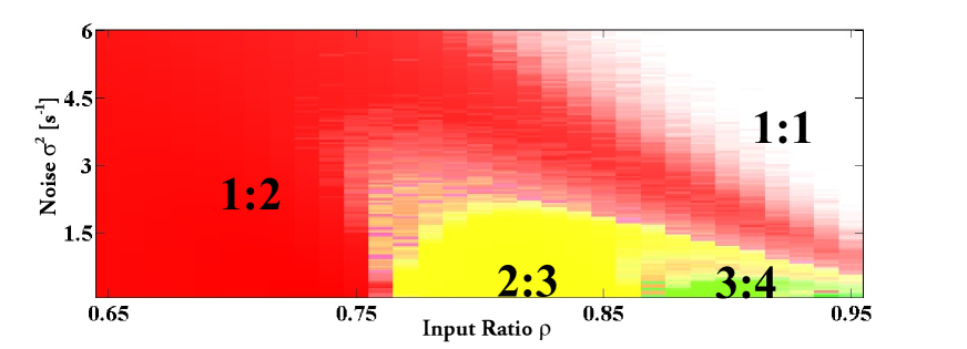
Figure 3: Phase diagram for a single network with periodic inhibition. Each neuron in the network receives independent noise. Parameters and colors as in Fig.2I.

To further our understanding we consider the impact of strictly periodic inhibition on the slower network 2 (Fig.1B). We generate that inhibition using network 1, omitting its inhibition by network 2 and using noiseless input, which is 20% reduced to compensate for the reduced inhibition. The behavior of this simplified system is qualitatively very similar to that of the bidirectionally coupled networks (Fig.3). Again, as the noise is increased the system undergoes transitions between different phase-locked states and eventually reaches the synchronized $1:1$-state via an inverse period-doubling bifurcation.

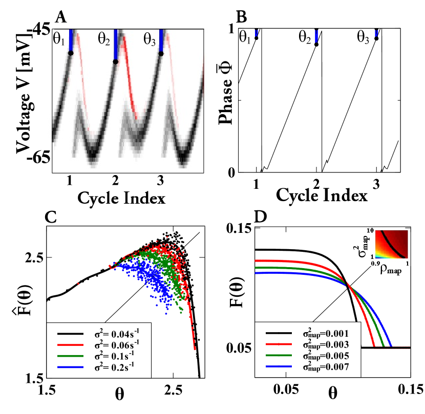
Figure 4: Network simulations (A,C) compared with results of the minimal map (B,D). Time-dependence of the voltage distribution (A) and of the mean phase $\bar{\phi}$ (B) and the lag $\theta$ of the activity of network 2. C) Iterated map extracted from direct simulations.. D) Iterated map from (6) and its slope at the fixed point (inset). Period-doubling bifurcation marked by line in inset. Parameters: (A,C) as in Fig.3 except $\rho=0.92$, $\sigma^{2}=1.8$ in (A) and $\rho=1.05$,$\gamma_{0}=1.9$ in (C); (B,D) $e^{-g_{1}}=0,$$e^{-g_{2}}=0.1,$$\tau_{d}=0.1$, $\rho_{map}=0.95$.

The temporal evolution of the voltage distribution of the neurons in network 2 provides insight into the synchronization mechanism (Figure 4A, darker color denotes larger number of neurons with that voltage). Not all neurons spike in each cycle: some do not reach the threshold before the periodic external inhibition sets in and keeps them from spiking (marked red in Fig.4A). Their voltage decreases smoothly instead of the instantaneous reset to $V_{r}$ after a spike. The fraction of neurons that spike varies from cycle to cycle. In the regime of interest the two peaks of the voltage distribution that correspond to spiking and non-spiking neurons are pushed together by the strong inhibition (Figure 4A) and before the neurons in network 2 spike again and before the next cycle of the periodic inhibition sets in the voltage distribution becomes unimodal. This allows us to develop a phenomenological Poincaré map for the mean phase $\bar{\phi}$ of the neurons. Assuming that the inhibition resets the phase of an oscillator by an amount proportional to the phase, we write the evolution of the mean phase as

$$\dot{\bar{\phi}}=-g_{1}P_{1}(t)\,\bar{\phi}(t)-g_{2}P_{2}(\bar{\phi}(t-\tau_{d}))\bar{\phi}(t)+\rho_{map},$$ (4)

with $\bar{\phi}$ being reset to $\bar{\phi}=0$ instantaneously when it reaches $\bar{\phi}=1$. The first term in (4) represents the periodic external forcing with strength $g_{1}$ and frequency 1. The second term models the self-inhibition of the network, which arises from those oscillators that are at the spike threshold when the average phase has the value $\bar{\phi}$. Their number is denoted by $P_{2}(\bar{\phi}(t))$. It reflects the phase distribution of the oscillators and the resulting heterogeneity in the spiking times. The simulations indicate that this heterogeneity plays a central role (Fig.4A). Instead of considering an evolution equation for this distribution, for our minimal model we consider it time-independent and of the form

$$P_{2}(\bar{\phi})=\left\{\begin{array}[]{cc}\frac{1}{\sigma_{map}}&\qquad\bar{\phi}\in[0,\frac{1}{2}\sigma_{map}]\cup[1-\frac{1}{2}\sigma_{map},1)\\ 0&\mbox{otherwise.}\end{array}\right.$$ (5)

Thus, for $\bar{\phi}\in[0,\sigma_{map}/2]$ neurons in the trailing half of the distribution are firing, while for $\bar{\phi}\in[1-\sigma_{map}/2,1)$ neurons in the leading half are firing.

Letting $t_{k}^{(2)}$ be the time at which the mean phase $\bar{\phi}$ reaches threshold, we focus on the situation in which the external inhibition arrives before any of the self-inhibition triggered by the oscillators in network 2 sets in, $t_{k}^{(1)}+\tau_{d}<t_{k}^{(2)}-\sigma_{map}/\left(2\rho_{map}\right)+\tau_{d}$. The external inhibition induces a phase reset $\bar{\phi}(t_{k}^{(1)}+\tau_{d})\rightarrow e^{-g_{1}}\bar{\phi}(t_{k}^{(1)}+\tau_{d})$. For sufficiently strong coupling $g_{1}$ it keeps the trailing oscillators from spiking and from contributing to the self-inhibition. Thus, self-inhibition lasts from $t_{k}^{<}=t_{k}^{(2)}-\sigma_{map}/2$ to $t_{k}^{>}=\min(t_{k}^{(1)}+\tau_{d},t_{k}^{(2)}+\sigma_{map}/\left(2\rho_{map}\right)+\tau_{d})$. During that time $\Delta t$ it induces a phase change that leads to

$$\bar{\phi}(t_{k}^{>})=e^{-g_{2}\frac{\rho_{map}\,\Delta t}{\sigma_{map}}}\phi(t_{k}^{<})+\frac{\sigma_{map}}{g_{2}}(1-e{}^{-g_{2}\frac{\rho_{map}\,\Delta t}{\sigma_{map}}}).$$ (6)

Combining (6) with the phase evolution during the remaining time yields a Poincaré map for the phase lag $\theta_{k}\equiv 1-\bar{\phi}\left(t_{k}^{(1)}\right)$ of network 2 relative to the periodic inhibitory input, $\theta_{k+1}=F(\theta_{k})$ (Fig.4B,D). The fixed point $\theta_{FP}=F(\theta_{FP})$ corresponds to a 1:1 synchronized state. It is only stable for large widths $\sigma_{map}$ of the distribution $P_{2}$, i.e. for sufficiently strong noise, and becomes unstable via a period-doubling bifurcation as the noise is reduced, capturing a striking, common feature of the full network simulations (Figs. 2D,3D).

The phase lag of network 2 relative to the periodic forcing extracted from the full simulations yields a noisy map that also undergoes a period-doubling bifurcation as the noise is increased (Fig.4C). Also captured by the phenomenological map is the simulation result that the noise level needed to stabilize the synchronized state increases with decreasing $\rho$, i.e. with increasing difference in the frequencies of the uncoupled networks (inset Fig.4D).

The minimal model (4,5) identifies as a key element of the synchronization the phase-dependent spiking fraction of network 2. Even though all neurons in this network receive the same mean external input, the noise in that input induces a spread in the phase. This allows the strong inhibition from network 1 or from the periodic forcing to suppress the spiking of the neurons that happen to be in the tail of the phase distribution, while the neurons in the front escape that inhibition. With fewer neurons spiking, the total self-inhibition within network 2 is reduced, speeding up the rhythm of network 2 in the following cycle. If the rhythm of network 2 is faster, more of its neurons spike, increasing self-inhibition and slowing down the rhythm. If this stabilizing feedback is removed by adjusting in each cycle the strength of the self-inhibition to compensate for the variable fraction $f_{s}$ of spiking neurons, $G_{syn}\rightarrow G_{syn}/f_{s}$, synchronization is lost (data not shown).

What functional consequences may the synchronization of rhythms by independent noise entail? Since it renders the spike timing of the neurons in network 2 more consistent relative to the spikes in network 1, it may, for instance, impact learning processes that are based on spike-timing dependent plasticity (STDP), an essential component of learning in the nervous system. We therefore consider a read-out neuron that is driven by both networks via synapses exhibiting STDP. To obtain the required excitatory outputs in a biologically convincing fashion our minimal inhibitory network would have to be extended to include also excitatory neurons BoKo03 . For simplicity we assume here that the spiking of the excitatory neurons in such an E-I network is sufficiently tightly correlated with the spiking of the inhibitory neurons that we can take the output of the inhibitory neurons as a proxy for the excitatory output.

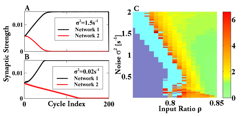
Figure 5: Learning is accelerated by independent noise. (A,B) Temporal evolution of the mean synaptic weight of the output synapses of network 1 and 2 with and without noise. (C) Learning duration $T_{l}$ as a function of noise and input ratio $\rho$. Light Blue: $T_{l}>6.7s$. Purple : synaptic weights increase rather than decrease. Parameters: $A_{p}=A_{m}=3\cdot 10^{-5}$, $\tau_{p}=\tau_{m}=5\mbox{ms}$ and as in Fig.2.

For the plastic synapses we take the STDP rule BiPo98

$$\Delta G=\left\{\begin{aligned} A_{p}e^{-(t_{post}-t_{pre})/\tau_{p}}&\mbox{ for }&t_{post}-t_{pre}>0\\ -A_{m}e^{(t_{post}-t_{pre})/\tau_{m}}&\mbox{ for }&t_{post}-t_{pre}<0\end{aligned}\right.$$ (7)

where $\Delta G$ is the change in the synaptic weight $G_{syn}$ when the read-out neuron spikes at $t_{post}$. The spike time of the respective pre-synaptic neuron is denoted by $t_{pre}$. For each presynaptic neuron each postsynaptic spike is paired with only adjacent presynaptic spikes. The weights $G_{syn}$ are restricted to $0\leq G_{syn}\leq 0.015$.

When two networks with slightly different intrinsic frequencies are coupled, the spikes of the faster network consistently precede the spikes of the read-out neuron, independent of the degree of synchronization of the two rhythms. This induces a monotonic increase in the weights of the output synapses of the faster network (Fig.5). This is, however, not the case for the slower network. Without synchronization and after a transient some of its spikes arrive after and some before the spikes of the read-out neuron. The resulting non-monotonic change in the synaptic weights slows down their overall decay (Fig.5A). However, when the rhythms of the two networks are synchronized by independent noise the neurons in the slower network always spike after the read-out neuron, resulting in a much faster decay of their synaptic weights. Thus, the synchronization by independent noise can enhance the speed with which read-out neurons select between different input networks.

The learning duration, defined as the time it takes for the mean of the output weights of the slower network to decay to $3\cdot 10^{-4}$, reflects in detail the tongue structure of the phase diagram (compare Fig.5B with Fig.2I). A more detailed inspection shows that near the period-doubling bifurcation from the $1:1$-state to the $1:2$-state the learning duration exhibits a minimum (line in Fig.2I): while in the $1:1$-state a decrease in noise reduces the variability in the spike timing, a similar decrease in noise in the $1:2$-state increases the variability because it predominantly increases the period-doubling amplitude.

In conclusion, we have shown that independent noise can synchronize population rhythms of coupled inhibitory networks of spiking neurons. As the underlying mechanism we have identified the phase heterogeneity of the neurons that results from the noise, which allows the faster network to suppress the spiking of a fraction of the neurons in the slower network. Since this mechanism requires variability in the spiking fraction it can only operate in networks; individual neurons are not synchronized by the uncorrelated noise. In fact, when the network size is reduced below $\mathcal{O}(100)$ neurons, the synchronization deteriorates significantly, because silencing an individual neuron impacts the self-inhibition too much.

The nature of the synchronization mechanism suggests that heterogeneity of neuronal properties instead of noisy inputs should similarly enhance the synchronizability of population rhythms in coupled networks. Preliminary simulations indicate this to be the case.

We gratefully acknowledge support by grant NSF-CMMI1435358. This research was supported in part through the computational resources and staff contributions provided for the Quest high performance computing facility at Northwestern University.

References

- [1] F. Dörfler and F. Bullo. Synchronization in complex networks of phase oscillators: A survey. Automatica, 50(6):1539–1564, June 2014.
- [2] F. A. Rodrigues, T. K. D. M. Peron, P. Ji, and J. Kurths. The Kuramoto model in complex networks. Physics Reports-Review Section of Physics Letters, 610:1–98, January 2016.
- [3] R. A. York and R. C. Compton. Quasi-optical power combining using mutually synchronized oscillator arrays. IEEE Transactions on Microwave Theory and Techniques, 39(6):1000–1009, June 1991.
- [4] S.L. Brown, J. Joseph, and M. Stopfer. Encoding a temporally structured stimulus with a temporally structured neural representation. Nat Neurosci, 8(11):1568–1576, Nov 2005.
- [5] K. Wiesenfeld, P. Colet, and S. H. Strogatz. Synchronization transitions in a disordered Josephson series array. Phys. Rev. Lett., 76(3):404–407, January 1996.
- [6] M. A. Zhang, G. S. Wiederhecker, S. Manipatruni, A. Barnard, P. McEuen, and M. Lipson. Synchronization of micromechanical oscillators using light. Physical Review Letters, 109(23):233906, December 2012.
- [7] D. C. Michaels, E. P. Matyas, and J. Jalife. Mechanisms of sinoatrial pacemaker synchronization - a new hypothesis. Circulation Research, 61(5):704–714, November 1987.
- [8] C. Liu, D. R. Weaver, S. H. Strogatz, and S. M. Reppert. Cellular construction of a circadian clock: Period determination in the suprachiasmatic nuclei. Cell, 91(6):855–860, December 1997.
- [9] X.-J. Wang. Neurophysiological and computational principles of cortical rhythms in cognition. Physiol. Rev., 90(3):1195–1268, July 2010.
- [10] G. Buzsaki and E. W. Schomburg. What does gamma coherence tell us about inter-regional neural communication? Nature Neuroscience, 18(4):484–489, April 2015.
- [11] Pascal Fries. Rhythms for cognition: Communication through coherence. Neuron, 88:220–235, Oct 2015.
- [12] A.S. Pikovsky. In R.Z. Sagdeev, editor, Nonlinear and Turbulent Processes in Physics, page 1601. Harwood Academic, Singapore, 1984.
- [13] C. S. Zhou and J. Kurths. Noise-induced phase synchronization and synchronization transitions in chaotic oscillators. Physical Review Letters, 88(23):230602, June 2002.
- [14] J. Teramae and D. Tanaka. Robustness of the noise-induced phase synchronization in a general class of limit cycle oscillators. Physical Review Letters, 93(20):204103, November 2004.
- [15] E. Shea-Brown, K. Josic, De La Rocha J., and B. Doiron. Correlation and synchrony transfer in integrate-and-fire neurons: Basic properties and consequences for coding. Phys. Rev. Lett., 100(10):108102, March 2008.
- [16] Aushra Abouzeid and Bard Ermentrout. Correlation transfer in stochastically driven neural oscillators over long and short time scales. Phys Rev E Stat Nonlin Soft Matter Phys, 84(6 Pt 1):061914, Dec 2011.
- [17] György Buzsaki and Xiao-Jing Wang. Mechanisms of gamma oscillations. Annual Review of Neuroscience, Vol 35, 35:203–225, 2012.
- [18] M. A. Whittington, R. D. Traub, N. Kopell, N. Kopell, B. Ermentrout, and E. H. Buhl. Inhibition-based rhythms: experimental and mathematical observations on network dynamics. Int. J. Psychophysiol., 38:315, 2000.
- [19] N. Brunel and X. J. Wang. What determines the frequency of fast network oscillations with irregular neural discharges? I. Synaptic dynamics and excitation-inhibition balance. J. Neurophysiol., 90(1):415–430, July 2003.
- [20] C. Börgers and N. Kopell. Synchronization in networks of excitatory and inhibitory neurons with sparse, random connectivity. Neural Comput., 15(3):509–538, March 2003.
- [21] Paul Tiesinga and Terrence J. Sejnowski. Cortical enlightenment: Are attentional gamma oscillations driven by ING or PING? Neuron, 63(6):727–732, September 2009.
- [22] Conrado A Bosman, Jan-Mathijs Schoffelen, Nicolas Brunet, Robert Oostenveld, Andre M Bastos, Thilo Womelsdorf, Birthe Rubehn, Thomas Stieglitz, Peter De Weerd, and Pascal Fries. Attentional stimulus selection through selective synchronization between monkey visual areas. Neuron, 75:875–888, Sep 2012.
- [23] K. R. Neville and L. B. Haberly. Beta and gamma oscillations in the olfactory system of the urethane-anesthetized rat. J. Neurophysiol., 90(6):3921–3930, December 2003.
- [24] Leslie M. Kay and Philip Lazzara. How global are olfactory bulb oscillations? Journal of Neurophysiology, 104(3):1768–1773, Sep 2010.
- [25] G. G. Gregoriou, S. J. Gotts, H. H. Zhou, and R. Desimone. High-frequency, long-range coupling between prefrontal and visual cortex during attention. Science, 324(5931):1207–1210, May 2009.
- [26] M. J. Roberts, E. Lowet, N. M. Brunet, M. Ter Wal, P. Tiesinga, P. Fries, and P. De Weerd. Robust gamma coherence between macaque V1 and V2 by dynamic frequency matching. Neuron, 78(3):523–536, May 2013.
- [27] E. Ravasz, A. L. Somera, D. A. Mongru, Z. N. Oltvai, and A. L. Barabasi. Hierarchical organization of modularity in metabolic networks. Science, 297(5586):1551–1555, August 2002.
- [28] E. T. Bullmore and O. Sporns. Complex brain networks: graph theoretical analysis of structural and functional systems. Nature Reviews Neuroscience, 10(3):186–198, March 2009.
- [29] S.-F. Chow, S. D. Wick, and H. Riecke. Neurogenesis drives stimulus decorrelation in a model of the olfactory bulb. PLoS Comp. Biol., 8:e1002398, 2012.
- [30] Kurt A. Sailor, Matthew T. Valley, Martin T. Wiechert, Hermann Riecke, Gerald J. Sun, Wayne Adams, James C. Dennis, Shirin Sharafi, Guo-Li Ming, Hongjun Song, and Pierre-Marie Lledo. Persistent structural plasticity optimizes sensory information processing in the olfactory bulb. Neuron, 91(2):384–396, Jul 2016.
- [31] K. Park, Y.C. Lai, S. Gupte, and J.W. Kim. Synchronization in complex networks with a modular structure. Chaos, 16(1):015105, Mar 2006.
- [32] F. Sorrentino and E. Ott. Network synchronization of groups. Physical Review E, 76(5):056114, November 2007.
- [33] E. Oh, K. Rho, H. Hong, and B. Kahng. Modular synchronization in complex networks. Physical Review E, 72(4):047101, October 2005.
- [34] A. Arenas, A. Diaz-Guilera, J. Kurths, Y. Moreno, and C. S. Zhou. Synchronization in complex networks. Physics Reports-review Section of Physics Letters, 469(3):93–153, December 2008.
- [35] S. G. Guan, X. G. Wang, Y. C. Lai, and C. H. Lai. Transition to global synchronization in clustered networks. Physical Review E, 77(4):046211, April 2008.
- [36] G.Q. Bi and M.M. Poo. Synaptic modifications in cultured hippocampal neurons: dependence on spike timing, synaptic strength, and postsynaptic cell type. J Neurosci, 18(24):10464–10472, Dec 1998.