Many-body effects of Coulomb interaction on Landau levels in graphene

Abstract

In strong magnetic fields, massless electrons in graphene populate relativistic Landau levels with the square-root dependence of each level energy on its number and magnetic field. Interaction-induced deviations from this single-particle picture were observed in recent experiments on cyclotron resonance and magneto-Raman scattering. Previous attempts to calculate such deviations theoretically using the unscreened Coulomb interaction resulted in overestimated many-body effects. This work presents many-body calculations of cyclotron and magneto-Raman transitions in single-layer graphene in the presence of Coulomb interaction, which is statically screened in the random-phase approximation. We take into account self-energy and excitonic effects as well as Landau level mixing, and achieve good agreement of our results with the experimental data for graphene on different substrates. Important role of a self-consistent treatment of the screening is found.

I Introduction

Graphene, the monolayer two-dimensional carbon crystal, grants a possibility to study how a many-body system of massless Dirac electrons behave in electric and magnetic fields CastroNeto ; Goerbig ; Novoselov ; Orlita ; Basov ; Miransky . One of the most striking manifestations of the “relativistic” nature of graphene is the unconventional half-integer quantum Hall effect in strong magnetic field Novoselov . The role of Coulomb interaction in graphene in the quantum Hall regime is still a debatable and controversial topic Goerbig ; Iyengar ; Bychkov ; Barlas ; Roldan1 ; Shizuya1 ; Shizuya2 ; Gorbar ; Menezes ; Miller ; Luican ; Chae ; Yu ; Jiang1 ; Henriksen ; Jiang2 ; Chen ; Takehana ; Faugeras ; Berciaud ; Orlita ; Basov ; Miransky ; Shovkovy .

Landau levels of electrons in graphene have the non-equidistant energies Goerbig

$$E_{n}^{(0)}=\mathrm{sgn}(n)\frac{v_{\mathrm{F}}}{l_{H}}\sqrt{2|n|},\quad n=0,\pm 1,\pm 2,\ldots,$$ (1)

where $v_{\mathrm{F}}\approx 10^{6}\,\mbox{m/s}$ is the Fermi velocity, $l_{H}=\sqrt{c/|e|B}$ is the magnetic length (hereafter we set $\hbar\equiv 1$). Contrary to the case of a non-relativistic electron gas, the energies of cyclotron transitions between Landau levels in graphene are not protected by Kohn’s theorem Kohn against interaction induced corrections, as both predicted theoretically Iyengar ; Bychkov ; Barlas ; Roldan1 ; Shizuya1 ; Shizuya2 ; Gorbar ; Menezes ; Shovkovy and reported in experimental works Jiang1 ; Henriksen ; Jiang2 ; Chen ; Takehana ; Luican ; Chae ; Yu ; Berciaud ; Faugeras .

The following major signatures of Coulomb many-body effects are observed: a) the energy of $0\rightarrow 1$ or $-1\rightarrow 0$ (referred to as $\mathrm{T}_{1}$) cyclotron inter-Landau level transitions and that of $-1\rightarrow 2$ or $-2\rightarrow 1$ transitions ($\mathrm{T}_{2}$) have the ratio deviating from the single-particle prediction $1/(1+\sqrt{2})$ Jiang1 ; Henriksen ; Jiang2 ; b) the renormalized Fermi velocities $v_{\mathrm{F}}^{*}$ which characterize the energies of symmetric interband $-n\rightarrow n$ transitions (referred to as $\mathrm{L}_{n}$) measured in magneto-Raman scattering Berciaud ; Faugeras demonstrate significant dependence on magnetic field and on a substrate dielectric constant.

The existing theoretical calculations Iyengar ; Bychkov ; Barlas ; Roldan1 ; Shizuya1 ; Shizuya2 ; Menezes ; Faugeras of inter-Landau level transitions in graphene were carried out in the first order in Coulomb interaction, which implies using of the unscreened Coulomb interaction in all matrix elements Note1 . This results in the overestimation of many-body effects in comparison with the experimental data, as noted in Refs. Shizuya1 ; Shizuya2 ; Jiang1 ; Jiang2 ; Faugeras ; Chae .

In this article, we calculate the energies of the cyclotron and magneto-Raman transitions between Landau levels in graphene using the Coulomb interaction which is screened in the random-phase approximation in the static limit. We include exchange self-energy and excitonic contributions to the transition energies, as well as the Landau level mixing in the excitonic channel, and fit the experimental data Jiang1 ; Jiang2 ; Faugeras ; Berciaud with our calculations. Using the bare Fermi velocity $v_{\mathrm{F}}=0.85\times 10^{6}\,\mbox{m/s}$ and realistic dielectric constants, we have achieved much better agreement with both the magneto-Raman Berciaud ; Faugeras and cyclotron resonance Jiang1 ; Jiang2 experiments than in previous attempts of other authors, which had dealt with the unscreened interaction Shizuya1 ; Shizuya2 ; Jiang1 ; Faugeras . Moreover, we find the important role of a self-consistent suppression of the screening due to an upward renormalization of transition energies.

The article is organized as follows. Our theoretical model is introduced in Sec. II. The results of calculations are presented and the experimental data are fitted in Sec. III. Finally, the conclusions are made in Sec. IV.

II Theoretical model

II.1 Exchange self-energies

Most theoretical models of Coulomb many-body effects in graphene Iyengar ; Bychkov ; Barlas ; Roldan1 ; Shizuya1 ; Shizuya2 ; Gorbar ; Menezes ; Faugeras ; Shovkovy take into account three major contributions to the inter-Landau level transition energies: single-particle exchange self-energies of electron and hole, an excitonic shift due to electron-hole Coulomb attraction (also referred to as a vertex correction) and an electron-hole exchange energy. The latter contribution is principal in calculating dispersions of collective magnetoplasmon excitations Iyengar ; Bychkov ; Roldan1 ; Shizuya3 ; Berman ; Tahir ; Roldan2 ; Lozovik ; Roldan3 ; Goerbig , but vanishes for optically excited nearly zero-momentum electron-hole pairs, therefore we will not include it in our calculations.

Renormalization of single-particle energy levels is conventionally treated using the Hartree-Fock approximation and the unscreened Coulomb interaction. Omitting the Hartree term, which affects only electrostatics of a graphene layer, we get the single-particle energy levels

$$E_{n}^{\mathrm{(HF)}}=E_{n}^{(0)}+\Sigma_{n}^{\mathrm{(exch)}}$$ (2)

shifted due to the Fock exchange self-energies (see Refs. Iyengar ; Bychkov ; Roldan1 ; Faugeras for the details of calculations)

$$\Sigma_{n}^{\mathrm{(exch)}}=-\sum_{n^{\prime}k^{\prime}}f_{n^{\prime}}\langle\psi_{nk},\psi_{n^{\prime}k^{\prime}}|v|\psi_{nk},\psi_{n^{\prime}k^{\prime}}\rangle.$$ (3)

Here $f_{n^{\prime}}$ is the occupation number of the $n^{\prime}$-th Landau level ($0\leqslant f_{n^{\prime}}\leqslant 1$), $\langle\psi_{nk},\psi_{n^{\prime}k^{\prime}}|v|\psi_{nk},\psi_{n^{\prime}k^{\prime}}\rangle$ is the exchange matrix element of the Coulomb interaction $v$; the latter has the form $v(\mathbf{r})=e^{2}/\varepsilon|\mathbf{r}|$ in a surrounding medium with the dielectric constant $\varepsilon$. Each single-particle state $\psi_{nk}$ is specified by a Landau level number $n$ and a guiding center index $k=0,1,2,\ldots$, when we work in the symmetric gauge.

As known Iyengar ; Bychkov ; Barlas ; Roldan1 ; Shizuya1 ; Shizuya2 ; Gorbar , the self-energies (3) diverge logarithmically when calculating the sum over the filled Landau levels of negative energies, so the cutoff $n^{\prime}\geqslant-n_{\mathrm{c}}$ is required in order to obtain finite results. The value of $n_{\mathrm{c}}$ can be estimated by equating the concentration $gn_{\mathrm{c}}/2\pi l_{H}^{2}$ of electrons on $n_{\mathrm{c}}$ Landau levels (with taking into account the fourfold spin and valley degeneracy $g=4$) to that in the filled valence band of intrinsic graphene, $2/S_{0}$:

$$n_{\mathrm{c}}=\frac{\pi l_{H}^{2}}{S_{0}}\approx\frac{39600}{B\,\mbox{[T]}}.$$ (4)

Here $S_{0}=a^{2}\sqrt{3}/2$ is the area of graphene elementary cell, $a\approx 2.46\,\mbox{\AA}$. Separating the part of (3) which diverges in the $n_{\mathrm{c}}\rightarrow\infty$ limit, we get

$$\Sigma_{n}^{\mathrm{(exch)}}=\frac{e^{2}}{\varepsilon l_{H}}\left\{-\sqrt{\frac{n_{\mathrm{c}}}{2}}+\mathrm{sgn}(n)\frac{\sqrt{|n|}}{4\sqrt{2}}\ln\frac{n_{\mathrm{c}}}{|n|}\right\}+\mathcal{O}(1).$$ (5)

In the weak magnetic field limit $B\rightarrow 0$, (5) can be tracked to the well-known form of electron self-energy in graphene in the absence of magnetic field. The first term of (5) equals to the large negative constant part of the Hartree-Fock self-energy $-e^{2}p_{\mathrm{c}}/2\varepsilon$ Roldan1 ; Sokolik ; Hwang , where $p_{\mathrm{c}}=\sqrt{2\pi/S_{0}}$ is the cutoff momentum. The second term describes the logarithmic renormalization of the Fermi velocity Gonzalez ; CastroNeto

$$v_{\mathrm{F}}^{*}=v_{\mathrm{F}}+\frac{e^{2}}{4\varepsilon}\ln\frac{p_{c}}{p_{\mathrm{F}}},$$ (6)

where $p_{\mathrm{F}}$ is the Fermi momentum. Thus the exchange self-energies with and without magnetic field have the same cutoff dependencies up to the linear and logarithmic levels. The same result was obtained in Ref. Menezes by a different method.

II.2 Excitonic effects

An excitonic energy shift due to Coulomb attraction between electron on the $n_{1}$-th Landau level and hole on the $n_{2}$-th level is often calculated in the first order in Coulomb interaction Iyengar ; Shizuya1 ; Shizuya2 ; Faugeras ; Roldan1 :

$$\Delta E_{n_{1}n_{2}}^{\mathrm{(exc)}}=-\langle\Phi_{n_{1}n_{2}}|v|\Phi_{n_{1}n_{2}}\rangle,$$ (7)

where $|\Phi_{n_{1}n_{2}}\rangle$ is the noninteracting electron-hole (or magnetoexcitonic) state at zero momentum.

Eq. (7) is the simplification of the more general picture, where the mixing of different $n_{2}\rightarrow n_{1}$ transitions should occur in the excitonic ladder Iyengar ; Bychkov ; Lozovik . To take it into account, one must consider the Hamiltonian in the basis of noninteracting electron-hole states with the matrix elements given by

$$\langle\Phi_{n_{1}^{\prime}n_{2}^{\prime}}|H|\Phi_{n_{1}n_{2}}\rangle=\delta_{n_{1}n_{1}^{\prime}}\delta_{n_{2}n_{2}^{\prime}}(E_{n_{1}}-E_{n_{2}})$$

$$-\langle\Phi_{n_{1}^{\prime}n_{2}^{\prime}}|v|\Phi_{n_{1}n_{2}}\rangle,$$ (8)

and find its eigenvalues. Here $E_{n}$ are the single-particle energies which are already renormalized by Coulomb interaction.

Our estimates show that it is sufficient to consider only the mixing of $\mathrm{L}_{1}$ and $\mathrm{L}_{2}$ magneto-Raman transitions or $\mathrm{T}_{1}$ and $\mathrm{T}_{2}$ cyclotron transitions, and its major effect is a slight increase of the energy distance between these transition lines due to an interlevel repulsion. The mixing with higher lying transitions has an overall weak effect in the presence of the screening (although it was estimated to be significant in the absence of the screening at $\varepsilon\sim 1$ Lozovik ).

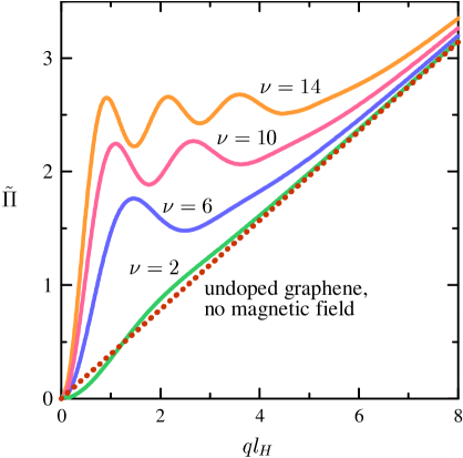
Figure 1: Dimensionless static polarizability of graphene in magnetic field $\tilde{\Pi}$ calculated in the random-phase approximation at zero temperature as functions of the dimensionless momentum $ql_{H}$. The filling factors $\nu=2,6,10,14$ correspond to complete fillings of, respectively, $n=0,1,2,3$ Landau levels. For comparison, polarizability of undoped graphene without magnetic field $\tilde{\Pi}=\pi ql_{H}/8$ is shown by the dotted line.

II.3 Screening of Coulomb interaction

Polarization of the electron gas in graphene, which can be described in terms of virtual electron-hole pairs, leads to the screening of Coulomb interaction. The screened interaction in the static limit $\omega\rightarrow 0$ is

$$V(q)=\frac{v(q)}{1-v(q)\Pi(q,0)},$$ (9)

where $v(q)=2\pi e^{2}/\varepsilon q$ is the two-dimensional Fourier transform of the unscreened interaction, and $\Pi(q,\omega)$ is the irreducible polarizability. In the random-phase approximation,

$$\Pi(q,0)=g\sum_{nn^{\prime}}F_{nn^{\prime}}(q)\frac{f_{n}-f_{n^{\prime}}}{E_{n}^{(0)}-E_{n^{\prime}}^{(0)}},$$ (10)

where $F_{nn^{\prime}}(q)$ are the Landau level form factors (see the details of polarizability calculations in Refs. Goerbig ; Gumbs ; Lozovik ; Pyatkovskiy ; Roldan2 ; Roldan3 ).

Introducing the positively valued dimensionless polarizability $\tilde{\Pi}(ql_{H})=-(2\pi v_{\mathrm{F}}l_{H}/g)\Pi(q,0)$, we get Eq. (9) in the form

$$V(q)=\frac{v(q)}{1+gr_{\mathrm{s}}\tilde{\Pi}(ql_{H})/ql_{H}},$$ (11)

where

$$r_{\mathrm{s}}=\frac{e^{2}}{\varepsilon v_{\mathrm{F}}}.$$ (12)

The dimensionless parameter $r_{\mathrm{s}}$ is conventionally used to characterize a relative strength of Coulomb interaction, but in our approach it appears only as a multiplier of $\tilde{\Pi}$ in the denominator of (11) and thus characterizes the relative strength of the screening. The case of unscreened Coulomb interaction corresponds to the zeroth order in this parameter, $r_{\mathrm{s}}=0$.

The numerically calculated polarizabilities are shown in Fig. 1 at different integer fillings $\nu$ of Landau levels ($\nu=0$ in undoped graphene and $\nu=4n+2$ when the $n$-th highest occupied level is completely filled). The functions $\tilde{\Pi}(ql_{H})$ oscillate at $ql_{H}\sim 1$ reflecting the nodal structure of Landau level wave functions and tend to the polarizability CastroNeto of undoped graphene without magnetic field $\tilde{\Pi}=\pi ql_{H}/8$ at $ql_{H}\gg 1$ (see also analysis in Gumbs ; Roldan3 ). Due to the electron-hole symmetry of the Dirac model, $\tilde{\Pi}$ does not depend on the sign of $\nu$. Remarkably, the same symmetry makes the polarizability independent on the filling of the 0-th Landau level, thus $\tilde{\Pi}$ is the same for $\nu=0$ and $\nu=\pm 2$, if we neglect intralevel electron transitions.

To improve calculations of the transition energies with taking into account the screening, we replace $v$ with (11) in the matrix elements of Coulomb interaction when calculate the electron self-energies (3) and treat excitonic effects (8):

$$\langle\Phi_{n_{1}^{\prime}n_{2}^{\prime}}|H|\Phi_{n_{1}n_{2}}\rangle=\delta_{n_{1}n_{1}^{\prime}}\delta_{n_{2}n_{2}^{\prime}}(E_{n_{1}}-E_{n_{2}})$$

$$-\langle\Phi_{n_{1}^{\prime}n_{2}^{\prime}}|V|\Phi_{n_{1}n_{2}}\rangle,$$ (13)

$$E_{n}=E_{n}^{(0)}-\sum_{\begin{subarray}{c}n^{\prime}k^{\prime}\\ n^{\prime}\geqslant-n_{\mathrm{c}}\end{subarray}}f_{n^{\prime}}\langle\psi_{nk},\psi_{n^{\prime}k^{\prime}}|V|\psi_{nk},\psi_{n^{\prime}k^{\prime}}\rangle.$$ (14)

Eqs. (10)–(14) compose the starting point of our numerical calculations.

III Calculation results and comparison with experiments

III.1 Magneto-Raman transitions

The recent experiments Berciaud ; Faugeras on magneto-Raman scattering showing clear signs of Coulomb many-body effects were carried out with undoped ($\nu=0$) graphene on three types of substrate: 1) suspended graphene, 2) graphene encapsulated in hexagonal boron nitride (hBN), 3) graphene on graphite. In each sample, the energies $E_{-1\rightarrow 1}$ and $E_{-2\rightarrow 2}$ of two transitions $\mathrm{L}_{1}$ and $\mathrm{L}_{2}$ were measured as functions of magnetic field in the range $2\div 25\,\mbox{T}$ and then converted to the renormalized Fermi velocities $v_{\mathrm{F}}^{*}$. The latter describe fictitious single-particle Landau levels (1) having the same energy difference: $2\sqrt{2n}v_{\mathrm{F}}^{*}/l_{H}=E_{-n\rightarrow n}$. The experimental points $v_{\mathrm{F}}^{*}(B)$ are reproduced in Fig. 2.

Our many-body calculations of $v_{\mathrm{F}}^{*}$ require the bare Fermi velocity $v_{\mathrm{F}}$ and the dielectric constant $\varepsilon$ as input parameters. Otherwise, these quantities can be obtained by least square fitting of experimental points. Generally, the best approximations to the experimental data can be achieved by independent adjustment of $v_{\mathrm{F}}$ and $\varepsilon$ for each of six transition lines in Fig. 2. We use more realistic fitting procedure, adjusting separate values of $\varepsilon$ for the pair of transitions $\mathrm{L}_{1,2}$ in each graphene sample as well as a common $v_{\mathrm{F}}$ for all samples.

Our attempts to fit the experimental data in different approximations (see below) show that the optimal value of common $v_{\mathrm{F}}$ is about $0.85\times 10^{6}\,\mbox{m/s}$. Smaller or larger values of $v_{\mathrm{F}}$ do not allow us to reproduce the slopes of experimental dependencies of $v_{\mathrm{F}}^{*}$ on $\ln\sqrt{B/B_{0}}$ accurately enough for all samples simultaneously. Assuming this $v_{\mathrm{F}}$, then we adjust the effective dielectric constant $\varepsilon$ for each graphene sample in order to achieve the best least square fit for its pair $\mathrm{L}_{1,2}$ of transitions. In agreement with the experiment, our calculations show that $v_{\mathrm{F}}^{*}$ for $\mathrm{L}_{2}$ is always higher than for $\mathrm{L}_{1}$ in the same sample, and dependencies of $v_{\mathrm{F}}^{*}$ on $\ln\sqrt{B/B_{0}}$ are approximately linear.

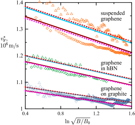
Figure 2: Renormalized Fermi velocities $v_{\mathrm{F}}^{*}$ as functions of magnetic field $B$ (the reference field strength is $B_{0}=1\,\mbox{T}$). Diamonds and triangles: experimental points from Ref. Faugeras for $\mathrm{L}_{1}$ and $\mathrm{L}_{2}$ transitions in three graphene samples. Solid and dotted lines: calculations with, respectively, unscreened and screened Coulomb interactions (see their parameters in Table 1) for the same pair of transitions in each sample.

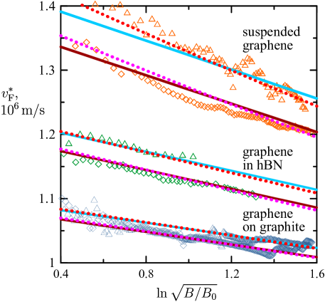
Figure 3: The same as Fig. 2, but solid and dotted lines present calculations with a “self-consistent” screening using, respectively, constant and varying $r_{\mathrm{s},n}$ (see the calculation parameters in Table 1).

First, we make the adjustment of $\varepsilon$ using the unscreened interaction, with the results shown in Fig. 2 (solid lines) and Table 1 (first column). The obtained $\varepsilon$ turned out to be too large in comparison with the actual dielectric constants of suspended graphene ($\varepsilon\approx 1$) and graphene in hBN ($\varepsilon\approx 4.5$) because they need to mimic the screening caused by both surrounding medium and graphene electrons. Besides, the distance between the $\mathrm{L}_{1}$ and $\mathrm{L}_{2}$ lines is clearly insufficient in this approximation. The same conclusions was made in Ref. Faugeras , where $\varepsilon$ was adjusted to approximate the slopes of experimental dependencies of $v_{\mathrm{F}}^{*}$ on $\ln\sqrt{B/B_{0}}$ and additional fictitious $\varepsilon_{\delta v}$ was needed to reproduce the interline distance in each sample.

Then we use the statically screened interaction and obtain the fitting results shown in Fig. 2 (dotted lines) and Table 1 (second column). Although we still have insufficient interline distances, the resulting $\varepsilon$ are no longer overestimated with respect to the actual ones, but are even underestimated (for example, $\varepsilon$ is even unphysically smaller than 1 in the case of suspended graphene). A possible reason is overestimation of the screening in the static limit in comparison with a full dynamical screening.

In order to improve agreement between theory and experiment, we can make the screening approximately “self-consistent”. Indeed, if the renormalized Fermi velocity $v_{\mathrm{F}}^{*}\approx(1.05\div 1.4)\times 10^{6}\,\mbox{m/s}$, which describes observable energies of inter-Landau level transitions, is 25%–65% higher than the bare velocity $v_{\mathrm{F}}=0.85\times 10^{6}\,\mbox{m/s}$, then the polarizability $\Pi(q,0)$ should correspondingly be renormalized to lower values due to increased energy denominators in (10). Since a full self-consistent treatment of renormalized transition energies in the polarizability would be computationally demanding and beyond the accuracy level of the static random-phase approximation, we resort to a simplified semi-phenomenological approach. We still use the same dimensionless $\tilde{\Pi}(ql_{H})$ (see Fig. 1), which describes qualitative features of the screening, but change the value of the parameter $r_{\mathrm{s}}$, which determines quantitatively the overall screening strength. For each transition $\mathrm{L}_{n}$ in each sample, we substitute an averaged (over the magnetic field range) value of experimental $v_{\mathrm{F}}^{*}$ instead of the bare $v_{\mathrm{F}}$ into the formula (12): $r_{\mathrm{s},n}=e^{2}/\varepsilon\langle v_{\mathrm{F},n}^{*}\rangle$. This replacement reduces the resulting $r_{\mathrm{s},n}$ and effectively weakens the screening.

The results of this approach are shown in Fig. 3 (solid lines) and Table 1 (third column). Increased interline distances provide much better agreement with the experimental data, that indicates importance of a self-consistent treatment of the screening.

We can improve agreement with the experiment even further, if take into account significant change of $v_{\mathrm{F},n}^{*}$ in the experimental range of magnetic field, which is most noticeable in the case of suspended graphene. In this fourth approximation, we assume $r_{\mathrm{s},n}=e^{2}/\varepsilon v_{\mathrm{F},n}^{*}(B)$, where $v_{\mathrm{F},n}^{*}(B)$ is the linear fit to experimental data for the $\mathrm{L}_{n}$ transition. The results, shown in Fig. 3 (dotted lines) and Table 1 (fourth column), demonstrate the best agreement with the experiment both in line slopes and interline distances.

	Unscreened	Screened	Self-consistent	Self-consistent
Sample	interaction	interaction	screening	screening
	$r_{\mathrm{s},n}=0$	$r_{\mathrm{s},n}=e^{2}/\varepsilon v_{\mathrm{F}}$	$r_{\mathrm{s},n}=e^{2}/\varepsilon\langle v_{\mathrm{F},n}^{*}\rangle$	$r_{\mathrm{s},n}=e^{2}/\varepsilon v_{\mathrm{F},n}^{*}(B)$
Suspended graphene	14.88	0.90	2.20	2.22
Graphene in hBN	17.41	3.41	4.47	4.48
Graphene on graphite	11.16	7.14	7.87	7.88

Table 1: Dielectric constants of surrounding media, obtained by least square fittings of magneto-Raman experimental data from Ref. Faugeras for each graphene sample at $v_{\mathrm{F}}=0.85\times 10^{6}\,\mbox{m/s}$. The fittings are carried out in four different theoretical approximations (see the text), and the corresponding screening parameters $r_{\mathrm{s},n}$ for each transition $\mathrm{L}_{n}$, which are used in these approximations, are shown.

III.2 Cyclotron transitions

Experimental data Jiang1 ; Jiang2 on the energies of cyclotron $\mathrm{T}_{1}$ and $\mathrm{T}_{2}$ transitions in graphene are depicted in Fig. 4 together with their linear fits $E\propto\sqrt{B}$. In these experiments, graphene is placed onto a $\mathrm{SiO}_{2}$ substrate and is electrostatically doped up to a complete filling of the $n=0$ ($\nu=2$) or $n=-1$ ($\nu=-2$) Landau level. The many-body effects are seen in deviation of the $\mathrm{T}_{2}$ energies from the $\mathrm{T}_{1}$ ones multiplied by $1+\sqrt{2}$ (dashed line in Fig. 4).

Our fits of the whole set of experimental points obtained by adjustment of $\varepsilon$ at fixed $v_{\mathrm{F}}=0.85\times 10^{6}\,\mbox{m/s}$ in different approximations are described in Table 2. In the case of unscreened interaction, we get, as before, overestimated $\varepsilon$ and insufficient interline distance (i.e. the difference between $v_{\mathrm{F}}^{*}$ for $\mathrm{T}_{1}$ and $\mathrm{T}_{2}$ is smaller than in the experiment). Taking into account the screening, we obtain much lower $\varepsilon$ and still insufficient interline distance. Finally, self-consistent treatment of the screening improves agreement with the experiments, as shown by dotted lines in Fig. 4.

	Experiment	Unscreened	Screened	Self-consistent
	Jiang1 ; Jiang2	interaction	interaction	screening
		$r_{\mathrm{s},n}=0$	$r_{\mathrm{s},n}=e^{2}/\varepsilon v_{\mathrm{F}}$	$r_{\mathrm{s},n}=e^{2}/\varepsilon\langle v_{\mathrm{F}}^{*}(\mathrm{T}_{n})\rangle$
$\varepsilon$	—	6.84	2.81	3.86
$v_{\mathrm{F}}^{*}(\mathrm{T}_{1}),\>10^{6}\,\mbox{m/s}$	1.119	1.136	1.134	1.131
$v_{\mathrm{F}}^{*}(\mathrm{T}_{2}),\>10^{6}\,\mbox{m/s}$	1.186	1.165	1.168	1.171

Table 2: First line: optimal dielectric constants $\varepsilon$ of surrounding media, obtained by least square fittings of the cyclotron resonance experimental data from Refs. Jiang1 ; Jiang2 at $v_{\mathrm{F}}=0.85\times 10^{6}\,\mbox{m/s}$ in different approximations. Second and third lines: the renormalized Fermi velocities $v_{\mathrm{F}}^{*}$, which are extracted from the experimental data and calculated at optimal $\varepsilon$ on average over the experimental magnetic field range.

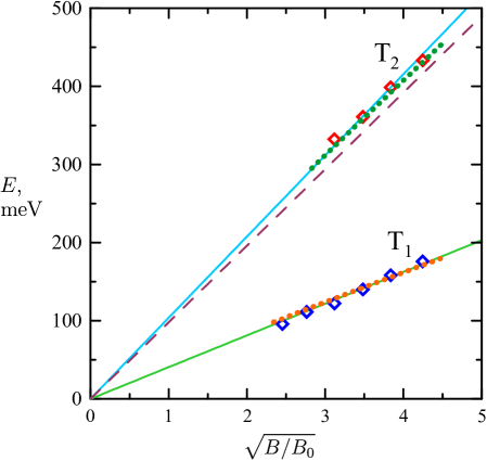
Figure 4: Energies of $\mathrm{T}_{1}$ and $\mathrm{T}_{2}$ cyclotron transitions as functions of square root of magnetic field (in the units of $B_{0}=1\,\mbox{T}$). Diamonds: the experimental data Jiang1 ; Jiang2 , solid lines: the linear fits to the experimental points (see Table 2, first column), dotted lines: the best theoretical fit with the self-consistent screening (see Table 2, last column). Dashed line: the $\mathrm{T}_{1}$ linear fit, multiplied by $1+\sqrt{2}$, which must pass through the $\mathrm{T}_{2}$ points in the absence of many-body effects.

IV Conclusions

We present a theoretical study of many-body effects of Coulomb interaction in graphene in strong magnetic field. Calculating the energies of the experimentally observable inter-Landau level transitions, we consider the single-particle self-energies, the excitonic effects, and the Landau level mixing. Moreover, this work presents the first systematic calculation which takes into account the screening of the Coulomb interaction and is aimed on detailed comparison with experiments.

The analysis of the experimental data Berciaud ; Faugeras on magneto-Raman $\mathrm{L}_{1}$ and $\mathrm{L}_{2}$ transitions in graphene on three different substrates has resulted in the following conclusions:

a) The optimal value of the bare Fermi velocity is about $v_{\mathrm{F}}=0.85\times 10^{6}\,\mbox{m/s}$, in agreement with the estimates $(0.8\div 0.9)\times 10^{6}\,\mbox{m/s}$ of this quantity based on analysis of recent experimental data Yu ; Hwang2 ; Faugeras ; Lozovik2 .

b) Calculations with the unscreened Coulomb interaction require too large dielectric constants $\varepsilon$ to obtain the best least square fits of experimental points and cannot accurately reproduce the distances between $\mathrm{L}_{1}$ and $\mathrm{L}_{2}$ spectral lines.

c) Static screening of the interaction yields too low values of $\varepsilon$ and also underestimates the interline distances.

d) Self-consistent treatment of the screening, which approximately models renormalization of transition energies in electron polarizability Note2 , greatly improves agreement of calculations with the experiment. The best fits are achieved when $\varepsilon\approx 2.2$ for suspended graphene, $\varepsilon\approx 4.5$ for graphene in hBN, and $\varepsilon\approx 8$ for graphene on graphite.

The similar conclusions are made from analysis of the experiments Jiang1 ; Jiang2 on cyclotron $\mathrm{T}_{1}$ and $\mathrm{T}_{2}$ transitions in graphene on a $\mathrm{SiO}_{2}$ substrate. Our best theoretical fit is achieved with the self-consistent screening at $v_{\mathrm{F}}=0.85\times 10^{6}\,\mbox{m/s}$ and $\varepsilon\approx 3.9$.

To conclude, we analyze the experimental data on many-body signatures in inter-Landau level transitions in graphene in strong magnetic fields. We show that taking into account the self-consistent screening of Coulomb interaction plays the key role in achieving agreement between the theory and experiments.

Our approach will be further developed by considering dynamical effects in the interaction screening in a subsequent work. It is also interesting to analyze possible signatures of Coulomb many-body effects observed in graphene on SiC Miller , hBN Chen , GaAs, and glass Takehana substrates in strong magnetic fields.

References

- (1) A. H. Castro Neto, F. Guinea, N. M. R. Peres, K. S. Novoselov, and A. K. Geim, The electronic properties of graphene, Rev. Mod. Phys. 81, 109 (2009).
- (2) K. S. Novoselov, A. K. Geim, S. V. Morozov, D. Jiang, M. I. Katsnelson, I. V. Grigorieva, S. V. Dubonos, and A. A. Firsov, Two-dimensional gas of massless Dirac fermions in graphene, Nature 438, 197 (2005).
- (3) M. O. Goerbig, Electronic properties of graphene in a strong magnetic field, Rev. Mod. Phys. 83, 1193 (2011).
- (4) M. Orlita and M. Potemski, Dirac electronic states in graphene systems: optical spectroscopy studies, Semicond. Sci. Technol. 25, 063001 (2010).
- (5) D. N. Basov, M. M. Fogler, A. Lanzara, F. Wang, and Y. Zhang, Colloquium: Graphene spectroscopy, Rev. Mod. Phys. 86, 959 (2014).
- (6) V. A. Miransky and I. A. Shovkovy, Quantum field theory in a magnetic field: From quantum chromodynamics to graphene and Dirac semimetals, Phys. Rep. 576, 1 (2015).
- (7) A. Iyengar, J. Wang, H. A. Fertig, and L. Brey, Excitations from filled Landau levels in graphene, Phys. Rev. B 75, 125430 (2007).
- (8) Yu. A. Bychkov and G. Martinez, Magnetoplasmon excitations in graphene for filling factors , Phys. Rev. B 77, 125417 (2008).
- (9) R. Roldán, J.-N. Fuchs, and M. O. Goerbig, Spin-flip excitations, spin waves, and magnetoexcitons in graphene Landau levels at integer filling factors, Phys. Rev. B 82, 205418 (2010).
- (10) Y. Barlas, W.-C. Lee, K. Nomura, and A. H. MacDonald, Renormalized Landau levels and particle-hole symmetry in graphene, Int. J. Mod. Phys. B 23, 2634 (2009).
- (11) K. Shizuya, Many-body corrections to cyclotron resonance in monolayer and bilayer graphene, Phys. Rev. B 81, 075407 (2010).
- (12) K. Shizuya, Many-body corrections to cyclotron resonance in graphene, J. Phys.: Conf. Ser. 334, 012046 (2011).
- (13) N. Menezes, V. S. Alves, and C. M. Smith, The influence of a weak magnetic field in the Renormalization-Group functions of (2+1)-dimensional Dirac systems, Eur. Phys. J. B 89, 271 (2016).
- (14) E. V. Gorbar, V. P. Gusynin, V. A. Miransky, and I. A. Shovkovy, Coulomb interaction and magnetic catalysis in the quantum Hall effect in graphene, Phys. Scr. T146, 014018 (2012).
- (15) I. A. Shovkovy and L. Xia, Generalized Landau level representation: Effect of static screening in the quantum Hall effect in graphene, Phys. Rev. B 93, 035454 (2016).
- (16) D. L. Miller, K. D. Kubista, G. M. Rutter, M. Ruan, W. A. de Heer, P. N. First, and J. A. Stroscio, Observing the Quantization of Zero Mass Carriers in Graphene, Science 324, 924 (2009).
- (17) A. Luican, G. Li, and E. Y. Andrei, Quantized Landau level spectrum and its density dependence in graphene, Phys. Rev. B 83, 041405(R) (2011).
- (18) J. Chae, S. Jung, A. F. Young, C. R. Dean, L. Wang, Y. Gao, K. Watanabe, T. Taniguchi, J. Hone, K. L. Shepard, P. Kim, N. B. Zhitenev, and J. A. Stroscio, Renormalization of the graphene dispersion velocity determined from scanning tunneling spectroscopy, Phys. Rev. Lett. 109, 116802 (2012).
- (19) G. L. Yu, R. Jalil, B. Belle, A. S. Mayorov, P. Blake, F. Schedin, S. V. Morozov, L. A. Ponomarenko, F. Chiappini, S. Wiedmann, U. Zeitler, M. I. Katsnelson, A. K. Geim, K. S. Novoselov, and D. C. Elias, Interaction phenomena in graphene seen through quantum capacitance, Proc. Natl. Acad. Sci. USA 110, 3282 (2013).
- (20) Z. Jiang, E. A. Henriksen, L. C. Tung, Y.-J. Wang, M. E. Schwartz, M. Y. Han, P. Kim, and H. L. Stormer, Infrared spectroscopy of Landau levels of graphene, Phys. Rev. Lett. 98, 197403 (2007).
- (21) Z. Jiang, E. A. Henriksen, P. Cadden-Zimansky, L.-C. Tung, Y.-J. Wang, P. Kim, and H. L. Stormer, Cyclotron resonance near the charge neutrality point of graphene, AIP Conf. Proc. 1399, 773 (2011).
- (22) E. A. Henriksen, P. Cadden-Zimansky, Z. Jiang, Z. Q. Li, L.-C. Tung, M. E. Schwartz, M. Takita, Y.-J. Wang, P. Kim, and H. L. Stormer, Interaction-induced shift of the cyclotron resonance of graphene using infrared spectroscopy, Phys. Rev. Lett. 104, 067404 (2010).
- (23) Z.-G. Chen, Z. Shi, W. Yang, X. Lu, Y. Lai, H. Yan, F. Wang, G. Zhang, and Z. Li, Observation of an intrinsic bandgap and Landau level renormalization in graphene/boron-nitride heterostructures, Nature Commun. 5, 4461 (2014).
- (24) K. Takehana, Y. Imanaka, T. Takamasu, Y. Kim, and K.-S. An, Substrate dependence of cyclotron resonance on large-area CVD graphene, Current Appl. Phys. 14, S119 (2014).
- (25) S. Berciaud, M. Potemski, and C. Faugeras, Probing electronic excitations in mono- to pentalayer graphene by micro magneto-Raman spectroscopy, Nano Lett. 14, 4548 (2014).
- (26) C. Faugeras, S. Berciaud, P. Leszczynski, Y. Henni, K. Nogajewski, M. Orlita, T. Taniguchi, K. Watanabe, C. Forsythe, P. Kim, R. Jalil, A. K. Geim, D. M. Basko, and M. Potemski, Landau level spectroscopy of electron-electron interactions in graphene, Phys. Rev. Lett. 114, 126804 (2015).
- (27) W. Kohn, Cycloron resonance and de Haas-van Alphen oscillations of an interacting electron gas, Phys. Rev. 123, 1242 (1961).
- (28) The exceptions are Refs. Gorbar ; Shovkovy , where various symmetry breaking scenarios in graphene in strong magnetic field were considered with taking into account the static screening of Coulomb interaction, but quantitative comparison with experimental data was not made.
- (29) K. Shizuya, Electromagnetic response and effective gauge theory of graphene in a magnetic field, Phys. Rev. B 75, 245417 (2007).
- (30) O. L. Berman, G. Gumbs, and Yu. E. Lozovik, Magnetoplasmons in layered graphene structures, Phys. Rev. B 78, 085401 (2008).
- (31) M. Tahir and K. Sabeeh, Inter-band magnetoplasmons in mono- and bilayer graphene, J. Phys.: Condens. Matter 20, 425202 (2008).
- (32) R. Roldán, J.-N. Fuchs, and M. O. Goerbig, Collective modes of doped graphene and a standard two-dimensional electron gas in a strong magnetic field: Linear magnetoplasmons versus magnetoexcitons, Phys. Rev. B 80, 085408 (2009).
- (33) Yu. E. Lozovik and A. A. Sokolik, Influence of Landau level mixing on the properties of elementary excitations in graphene in strong magnetic field, Nanoscale Res. Lett. 7, 134 (2012).
- (34) R. Roldán, M. O. Goerbig, and J.-N. Fuchs, The magnetic field particle-hole excitation spectrum in doped graphene and in a standard two-dimensional electron gas, Semicond. Sci. Technol. 25, 034005 (2010).
- (35) A. A. Sokolik, A. D. Zabolotskiy, and Yu. E. Lozovik, Generalized virial theorem for massless electrons in graphene and other Dirac materials, Phys. Rev. B 93, 195406 (2016).
- (36) E. H. Hwang, B. Y.-K. Hu, and S. Das Sarma, Density dependent exchange contribution to and compressibility in graphene, Phys. Rev. Lett. 99, 226801 (2007).
- (37) J. González, F. Guinea, and M. A. H. Vozmediano, Non-Fermi liquid behavior of electrons in the half-filled honeycomb lattice (A renormalization group approach), Nucl. Phys. B 424, 595 (1994).
- (38) P. K. Pyatkovskiy and V. P. Gusynin, Dynamical polarization of graphene in a magnetic field, Phys. Rev. B 83, 075422 (2011).
- (39) G. Gumbs, A. Balassis, D. Dahal, and M. L. Glasser, Thermal smearing and screening in a strong magnetic field for Dirac materials in comparison with the two dimensional electron liquid, Eur. Phys. J. B 89, 234 (2016).
- (40) C. Hwang, D. A. Siegel, S.-K. Mo, W. Regan, A. Ismach, Y. Zhang, A. Zettl, and A. Lanzara, Fermi velocity engineering in graphene by substrate modification, Sci. Rep. 2, 590 (2012).
- (41) Yu. E. Lozovik, A. A. Sokolik, and A. D. Zabolotskiy, Quantum capacitance and compressibility of graphene: The role of Coulomb interactions, Phys. Rev. B 91, 075416 (2015).
- (42) In other terms, the self-consistency of the screening in the random-phase approximation is the difference between the and approximations.