On Two-Component Dark-Bright Solitons in Three-dimensional Atomic Bose-Einstein Condensates

Abstract

In the present work, we revisit two-component Bose-Einstein condensates in their fully three-dimensional (3d) form. Motivated by earlier studies of dark-bright solitons in the 1d case, we explore the stability of these structures in their fully 3d form in two variants. In one the dark soliton is planar and trapping a planar bright (disk) soliton. In the other case, a dark spherical shell soliton creates an effective potential in which a bright spherical shell of atoms is trapped in the second component. We identify these solutions as numerically exact states (up to a prescribed accuracy) and perform a Bogolyubov-de Gennes linearization analysis that illustrates that both structures can be dynamically stable in suitable intervals of sufficiently low chemical potentials. We corroborate this finding theoretically by analyzing the stability via degenerate perturbation theory near the linear limit of the system. When the solitary waves are found to be unstable, we explore their dynamical evolution via direct numerical simulations which, in turn, reveal novel waveforms that are more robust. Finally, using the SO$(2)$ symmetry of the model, we produce multi-dark-bright planar or shell solitons involved in pairwise oscillatory motion.

I Introduction

Multi-component nonlinear waves have been explored in a variety of physical contexts kivshar ; stringari ; rip . Some of most prototypical ones among them, however, have been nonlinear optics kivshar , as well as atomic Bose-Einstein condensates (BECs) stringari ; rip . A relevant model in both cases is the one proposed by Manakov manakov ; intman1 , which has also been a theme of intense focus within mathematical physics due to its integrability ablowitz . This has generated the possibility of producing bright vector solitons in the case of self-focusing nonlinearities (in optics; self-attractive interactions in the atomic realm), and dark vector solitons for self-defocusing ones (self-repulsive interactions in the atomic case). In the latter case, also more exotic states such as the so-called dark-bright solitary waves siambook can be generated. Higher-dimensional variants of the latter will be a focal point of the present study.

Dark-bright solitary waves emerge in self-defocusing systems, although bright solitons generally are not possible in them, for a simple reason: dark solitons form a waveguiding potential that traps the light or matter (in optics or BECs, respectively) in the second component rip . The robustness of the resulting excitations enabled the pioneering observation of such states in photorefractive media in the works of seg1 ; seg2 . More recently, motivated by their theoretical prediction in an atomic (trapped) setting by buschanglin , a substantial number of experimental explorations emerged in the atomic realm hamburg ; pe1 ; pe2 ; pe3 ; pe4 ; pe5 ; azu . These addressed a diverse array of questions, including their ways of generation, e.g., via phase imprinting and counterflow among others hamburg ; pe1 ; pe4 , effects of dimensionality pe2 , their bound-state pairs pe3 ; lia , or interactions with external potentials azu . In parallel, to these, variants of the states such as the so-called dark-dark solitons arising due to the invariance of the Manakov model to SO$(2)$ rotation pe4 ; pe5 have also been extensively examined.

Most of the above mentioned studies on dark-bright solitary waves have been experimentally performed in setups that were higher than one-dimensional (1d) –although often the trapping was such that the system could be deemed to be, to a reasonable approximation, in a 1d regime. On the other hand, much of the theoretical analysis and especially the analytically available exact solutions christo ; vdbysk1 ; vddyuri ; ralak ; dbysk2 ; shepkiv ; parkshin are found in 1d settings. This naturally prompts the question: are there analogues of dark-bright solitons in genuinely higher dimensional settings and, if so, can they be stable –possibly in some appropriate parametric regimes? Our aim in the present work is to indicate that the answer to both questions can be positive, in fact, for multiple different installments of dark-bright solitary waves.

In particular, we examine one variant of a dark-bright soliton where the dark soliton is genuinely one-dimensional i.e., it represents a hyperbolic tangent solution along one of the systems axis, being homogeneous in the other two directions. This creates a dark soliton “plane”. The resulting planar effective potential, in the spirit of the standard dark-bright soliton, can trap a bright mass of light/atoms i.e., a planar bright soliton. We also explore a more three-dimensional installment of the relevant waveform motivated by the recent illustration of dark spherical shell (DSS) solitons dss , in which a DSS traps through its density dip a bright shell of atoms in the second component. In both cases, we examine these states in the presence of parabolic trapping as is customary in the realm of atomic BECs stringari ; rip ; siambook . Remarkably, we find that both of these patterns, both the planar dark bright (PDB) and the spherical dark bright (SDB) can be dynamically stable for suitable choices of chemical potentials. Nevertheless, as may be expected from their one-component analogues, both states have destabilization mechanisms that arise via a set of pitchfork (symmetry breaking) bifurcations that we analyze. These bifurcations are found to be interesting in their own right as they lead to the emergence of novel states (ones with multiple vortex-line-bright or vortex-ring-bright solitons stathis ) that are worthwhile to explore further. Hence, the usefulness of the present study extends to the identification of the latter states as well. Lastly, we utilize the SO$(2)$ symmetry of the Manakov model to produce variants of the PDB and SDB (in the same vein as the symmetry is used to produce dark-dark solitons from dark-bright ones pe4 ; pe5 ).

Our presentation of the above features will be structured as follows. In Sec. II we present the theoretical and numerical setup of the system and the associated methods of analysis. In Sec. III, we present our systematic numerical results and comparison with theoretical predictions. Finally, our conclusions and a number of open problems for future consideration are given in Sec. IV.

II Model and Computational Setup

II.1 The Gross-Pitaevskii equation

In the framework of mean-field theory, and for sufficiently low-temperatures, the dynamics of a two-component 3d repulsive BECs, confined by a time-independent trap $V$, is described by the following dimensionless Gross-Pitaevskii equation (GPE) [see siambook ; emergent for relevant reductions to dimensionless units]

$$i\frac{\partial\psi_{1}}{\partial t} = -\frac{1}{2}\nabla^{2}\psi_{1}+V\psi_{1}+(|\psi_{1}|^{2}+|\psi_{2}|^{2})\psi_{1}$$

$$i\frac{\partial\psi_{2}}{\partial t} = -\frac{1}{2}\nabla^{2}\psi_{2}+V\psi_{2}+(|\psi_{1}|^{2}+|\psi_{2}|^{2})\psi_{2},$$ (1)

where $\psi_{1}(x,y,z,t)$ and $\psi_{2}(x,y,z,t)$ are the macroscopic wavefunctions. We have in mind in the present setting a scenario of equal masses associated with the hyperfine states of the same gas (e.g., ⁸⁷Rb) rip . It is in that vein that we consider it to be a good approximation to assume that the scattering length ratios (for intercomponent and intracomponent interactions) are near unity opanchuk . Furthermore, we examine the typical (experimentally) case ofa harmonic trap of the form:

$$V=\frac{1}{2}\omega_{\rho}^{2}\rho^{2}+\frac{1}{2}\omega_{z}^{2}z^{2},$$ (2)

where $\rho=\sqrt{x^{2}+y^{2}}$, $\omega_{\rho}$ and $\omega_{z}$ are the trapping frequencies along the $x\textrm{-}y$ plane and the vertical direction $z$, respectively. Note that the potential has rotational symmetry with respect to the $z$-axis. In our numerical simulations, we focus on the isotropic (spherical) case with $\omega=\omega_{\rho}=\omega_{z}=1$.

In this system, we seek stationary states of the form

$$\psi_{1}(\vec{r},t) = \psi^{0}_{1}(\vec{r})e^{-i\mu_{1}t}$$

$$\psi_{2}(\vec{r},t) = \psi^{0}_{2}(\vec{r})e^{-i\mu_{2}t}$$ (3)

which, in turn, lead to the stationary equations:

$$-\frac{1}{2}\nabla^{2}\psi^{0}_{1}+V\psi^{0}_{1}+(|\psi^{0}_{1}|^{2}+|\psi^{0}_{2}|^{2})\psi^{0}_{1} = \mu_{1}\psi^{0}_{1}$$

$$-\frac{1}{2}\nabla^{2}\psi^{0}_{2}+V\psi^{0}_{2}+(|\psi^{0}_{1}|^{2}+|\psi^{0}_{2}|^{2})\psi^{0}_{2} = \mu_{2}\psi^{0}_{2},$$ (4)

where $\mu_{1}$ and $\mu_{2}$ are the chemical potentials of the first and second components, respectively. A theoretical analysis of the existence of solutions to Eqs. (II.1) can be presented in the vicinity of the vanishing amplitude limit where the problem becomes linear (and hence analytically tractable). We explore a perturbative analysis near this limit next.

II.2 The degenerate perturbation theory

The eigenstates and eigenvalues of Eqs. (II.1) in the linear limit are the eigenstates of the 3d quantum harmonic oscillator. We now seek to identify how these eigenstates and eigenvalues are modified by the presence of the nonlinearity as we depart from this limit. Near the limit, we apply the expansion for the eigenstates and eigenvalues as follows:

$$\psi_{1}^{0} = \sqrt{\epsilon}\psi_{10}+\epsilon^{3/2}\psi_{11}+\dots,$$

$$\psi_{2}^{0} = (\sqrt{\epsilon\eta}\psi_{20}+(\epsilon\eta)^{3/2}\psi_{22})\dots,$$

$$\mu_{1} = \mu_{10}+\epsilon\mu_{11}+\dots,$$

$$\mu_{2} = \mu_{20}+\epsilon\eta\mu_{22}+\dots,$$ (5)

where $\psi_{10},\psi_{20},\mu_{10}$ and $\mu_{20}$ are normalized simple harmonic oscillator eigenstates and eigenenergies of the first and second components, respectively; $\mu_{11}$ and $\mu_{22}$ are two parameters that need to be determined self-consistently using Eqs. (II.1). The parameter $\eta$ represents the ratio of the perturbations from the linear limit of the two components in the units of $\mu_{11}$ and $\mu_{22}$, respectively. $\eta$ depends on the selected path in the $(\mu_{1},\mu_{2})$ plane. We use a linear path and $\eta$ is $O(1)$ in our simulations.

To $O(\epsilon^{3/2})$, we get as a self-consistency condition from Eqs. II.1:

$$\mu_{11} = \int(|\psi_{10}|^{2}+\eta|\psi_{20}|^{2})|\psi_{10}|^{2}d^{3}x,$$

$$\mu_{22} = \frac{1}{\eta}\int(|\psi_{10}|^{2}+\eta|\psi_{20}|^{2})|\psi_{20}|^{2}d^{3}x.$$ (6)

We then define the slope of a linear path $s=\frac{\mu_{1}-\mu_{10}}{\mu_{2}-\mu_{20}}$ in the $(\mu_{1},\mu_{2})$ plane, and $I_{ij}=\int|\psi_{i0}|^{2}|\psi_{j0}|^{2}d^{3}x$, and note that $I_{12}=I_{21}$, then

$$\eta=\frac{I_{11}-sI_{12}}{sI_{22}-I_{12}}.$$ (7)

Next, we use this decomposition in order to identify the linear stability eigenvalues of perturbations around the equilibria of Eqs. (II.1). In this, so-called, Bogolyubov-de Gennes (BdG) analysis, we utilize the perturbation ansatz

$$\psi_{1} = e^{-i\mu_{1}t}\left[\psi_{1}^{0}+\delta\left(a(\vec{r})e^{\lambda t}+b^{\star}(\vec{r})e^{\lambda^{\star}t}\right)\right]$$ (8)

$$\psi_{2} = e^{-i\mu_{2}t}\left[\psi_{2}^{0}+\delta\left(c(\vec{r})e^{\lambda t}+d^{\star}(\vec{r})e^{\lambda^{\star}t}\right)\right]$$ (9)

and derive, to O$(\delta)$ the linearized equations $\lambda(a,b,c,d)^{T}=M(a,b,c,d)^{T}$ where the eigenvalues are denoted by $\lambda$, the eigenvectors by $(a,b,c,d)^{T}$ (^T stands for transpose) and the linearization matrix $M$ is given in Appendix A.

In the matrix $M$, if we separate the diagonal terms $-\frac{1}{2}\nabla^{2}+V-\mu_{1}$ into $-\frac{1}{2}\nabla^{2}+V-\mu_{10}-(\mu_{1}-\mu_{10})$ and $-\frac{1}{2}\nabla^{2}+V-\mu_{2}$ into $-\frac{1}{2}\nabla^{2}+V-\mu_{20}-(\mu_{2}-\mu_{20})$, the eigenvalues and eigenstates of the diagonal parts with $-\frac{1}{2}\nabla^{2}+V-\mu_{10}$ and $-\frac{1}{2}\nabla^{2}+V-\mu_{20}$ are known, and the rest of the terms are all $O(\epsilon)$ (upon the expansion of Eqs. (5)) hence they can be treated as perturbations. Therefore, one can apply the degenerate perturbation analysis order-by-order so as to identify the eigenvalues and eigenstates of the $M$ matrix. The basis we use consists of the simple harmonic oscillator states in the first, second, third and fourth elements of the $4\times 1$ vector space that we can call up-up states, up-down states, down-up states and down-down states. For example, for a simple harmonic oscillator state $|mnp\rangle$ with eigenvalue $E_{mnp}$, the four states are as ($|mnp\rangle,0,0,0)^{T}$, (0,$|mnp\rangle,0,0)^{T}$, ($0,0,|mnp\rangle,0)^{T}$ and ($0,0,0,|mnp\rangle)^{T}$, with eigenvalues $E_{mnp}-\mu_{10}$, $\mu_{10}-E_{mnp}$, $E_{mnp}-\mu_{20}$, $\mu_{20}-E_{mnp}$, with a factor of $-i$.

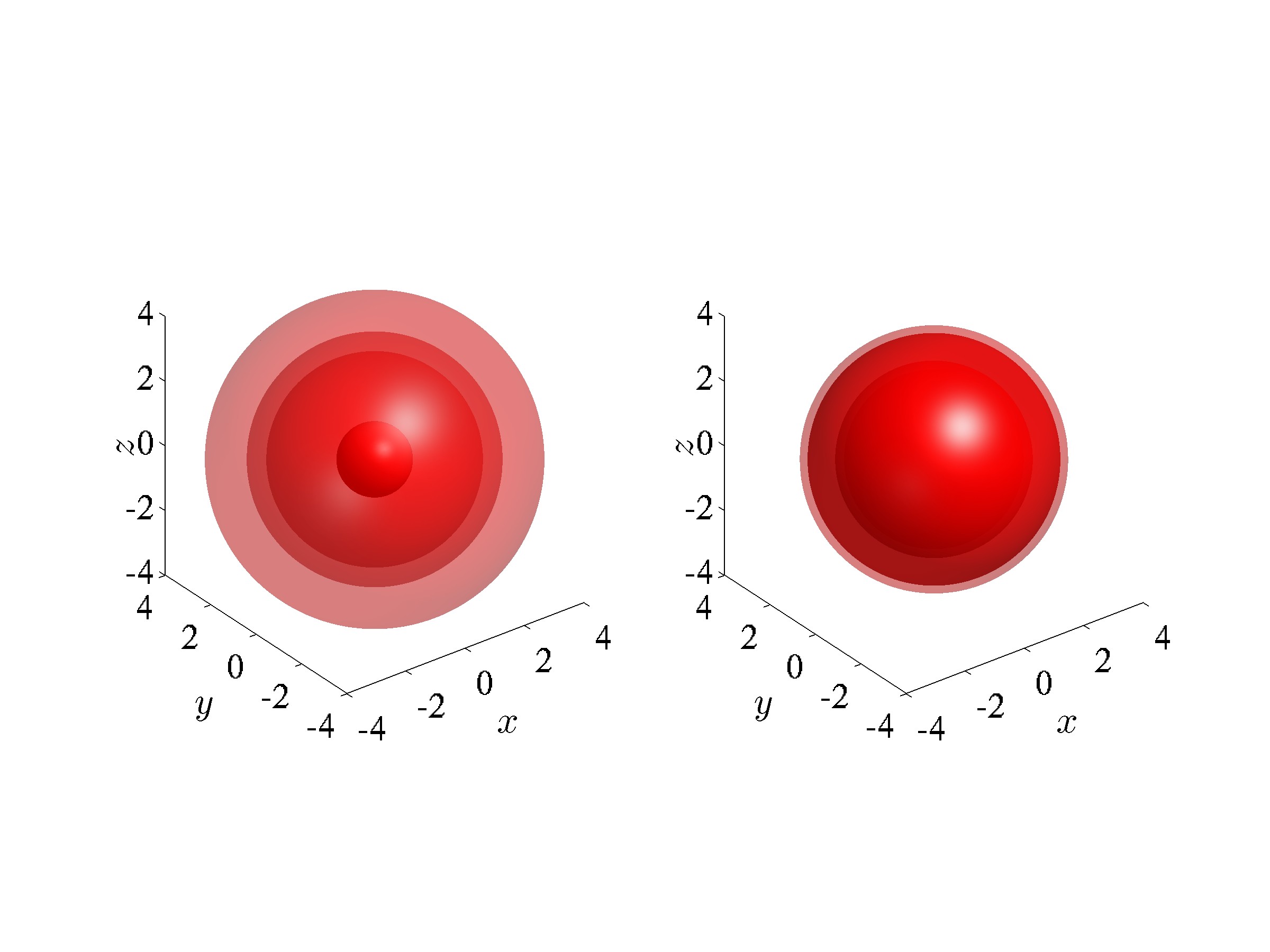
The principal nonlinear states that we consider in what follows are the PDB and SDB solitary waves. The former one (PDB) at the linear limit corresponds to a $\psi_{10}=|001\rangle$ state in the first component. This state, as nonlinearity increases, has been shown to morph into a planar dark soliton, as was discussed in russell . This is coupled for the PDB with the ground state $\psi_{20}=|000\rangle$ in the second component. On the other hand, for the SDB, as discussed in dss , the linear analogue of dark spherical shell is given by:

$$|\psi_{\rm{DSS}}\rangle_{\rm{linear}} = \frac{1}{\sqrt{3}}\left(|200\rangle+|020\rangle+|002\rangle\right)$$ (10)

$$\propto \left(\omega r^{2}-\frac{3}{2}\right)e^{-\omega r^{2}/2}.$$

Hence, we pick for the first component $\psi_{10}=\psi_{\rm{DSS}}$, while for the second component once again we select the ground state $\psi_{20}=|000\rangle$.

Then, within the realm of the degenerate perturbation theory (DPT), the relevant states for eigenvalues of the PDB and the SDB solitary waves near the spectrum of Im($\lambda$)=0, 1 and 2 (in units of the trapping frequency) are listed in Table 1. For the corresponding states, the O$(1)$ prediction of the DPT is Im($\lambda$)=0, 1 and 2, respectively, while the O$(\epsilon)$ prediction yields how these modes depart from the linear limit (in a way proportional to the perturbation size $\epsilon$). This prediction will be compared with the full numerical results from the linearization of the matrix $M$ in Sec. III.

Table 1: Relevant states for eigenvalues of the planar dark bright (PDB) and spherical dark bright (SDB) solitons near the spectrum of Im($\lambda$)=0, 1 and 2 for the degenerate perturbation theory. Here $|mnp\rangle$ stands for eigenstates with all possible distinct permutations with the quantum numbers $m,n$ and $p$.

Im($\lambda$)	States	“up-up” states	“up-down” states	“down-up” states	“down-down” states
$0$	PDB	$|001\rangle$	$|001\rangle$	$|000\rangle$	$|000\rangle$
$1$	PDB	$|002\rangle$ $|011\rangle$	$|000\rangle$	$|001\rangle$
$2$	PDB	$|003\rangle$ $|012\rangle$ $|111\rangle$		$|002\rangle$ $|011\rangle$
$0$	SDB	$|002\rangle$ $|011\rangle$	$|002\rangle$ $|011\rangle$	$|000\rangle$	$|000\rangle$
$1$	SDB	$|003\rangle$ $|012\rangle$ $|111\rangle$	$|001\rangle$	$|001\rangle$
$2$	SDB	$|004\rangle$ $|013\rangle$ $|022\rangle$ $|112\rangle$	$|000\rangle$	$|002\rangle$ $|011\rangle$

A detailed analysis of the numerical method (and its use of the symmetry of the solutions) is explained in Appendix B. For our current purposes, suffice it to say that we obtain the full solution of Eqs. (II.1) up to a prescribed tolerance via a 2d Newton iteration (our solutions will not have a topological charge –and hence a dependence on the azimuthal variables– in the cylindrical coordinates used for the PDB and SDB). Subsequently the BdG analysis is used, once again taking advantage of the symmetry of the solution as is detailed in Appendix B, and the numerical linearization spectrum of eigenvalues $\lambda$ is identified. The process is repeated for our prescribed parametric variation over $\mu$ and the resulting bifurcation as well as stability diagram will be presented in comparison with the corresponding near-linear theoretical prediction of the DPT.

III Numerical and analytical results

We now turn to the numerical investigation of our higher-dimensional dark-bright soliton states of interest.

III.1 The PDB and SDB spectrum

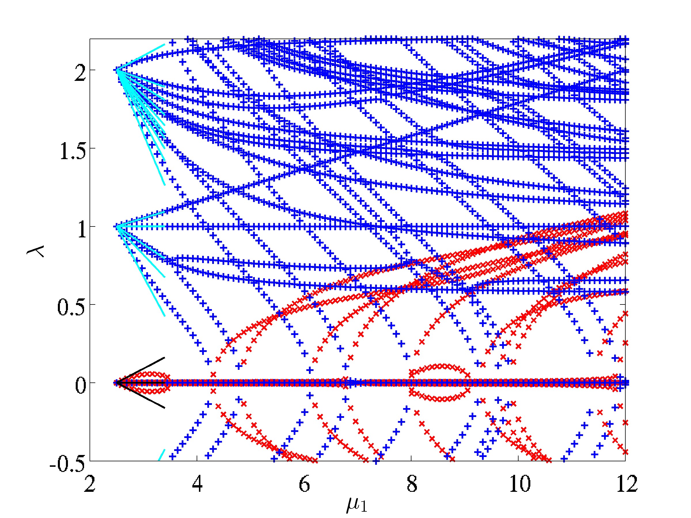
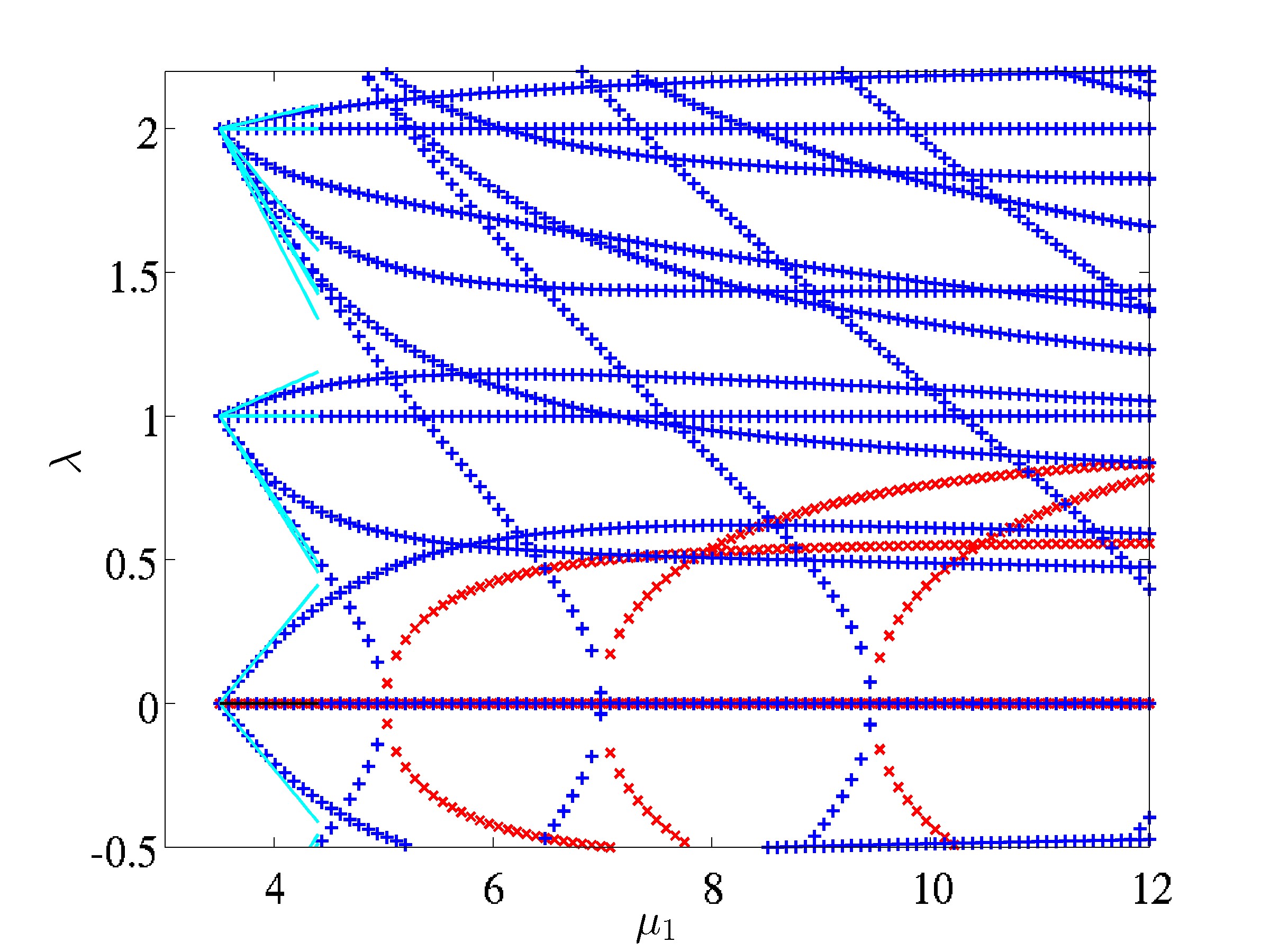
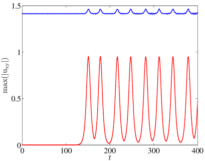
A typical stationary state and the spectrum of the PDB are shown in Fig. 1, and similarly for the SDB in Fig. 2. The figures also illustrate a continuation over a parametric line in the $(\mu_{1},\mu_{2})$ plane, in terms of the stability eigenvalues $\lambda$. It is interesting that in the case $\mu_{1}\approx\mu_{2}$, the qualitative features of the spectrum are similar to the dark soliton and the dark soliton shell in one component BECs, respectively. In particular, the planar DB similarly to the planar dark soliton is unstable very near the linear limit (an instability captured quite accurately –as are all eigenmodes near that limit– by the degenerate perturbation theory). On the other hand, the spherical DB similarly to the dark soliton shell state of dss is stable in the immediate vicinity of the linear limit, where once again the DPT fares very well in capturing the leading order behavior of the associated eigenmodes. Nevertheless, as mentioned earlier, both states present chemical potential intervals where the solitons are completely stable. In our simulations, we find they are stable in the intervals of $3.6<\mu_{1}<4.2$ and $3.5<\mu_{1}<4.9$ for PDB and SDB, respectively. These spectral stability conclusions of the BdG analysis have been confirmed through direct numerical computations using a 4th order Runge-Kutta scheme.

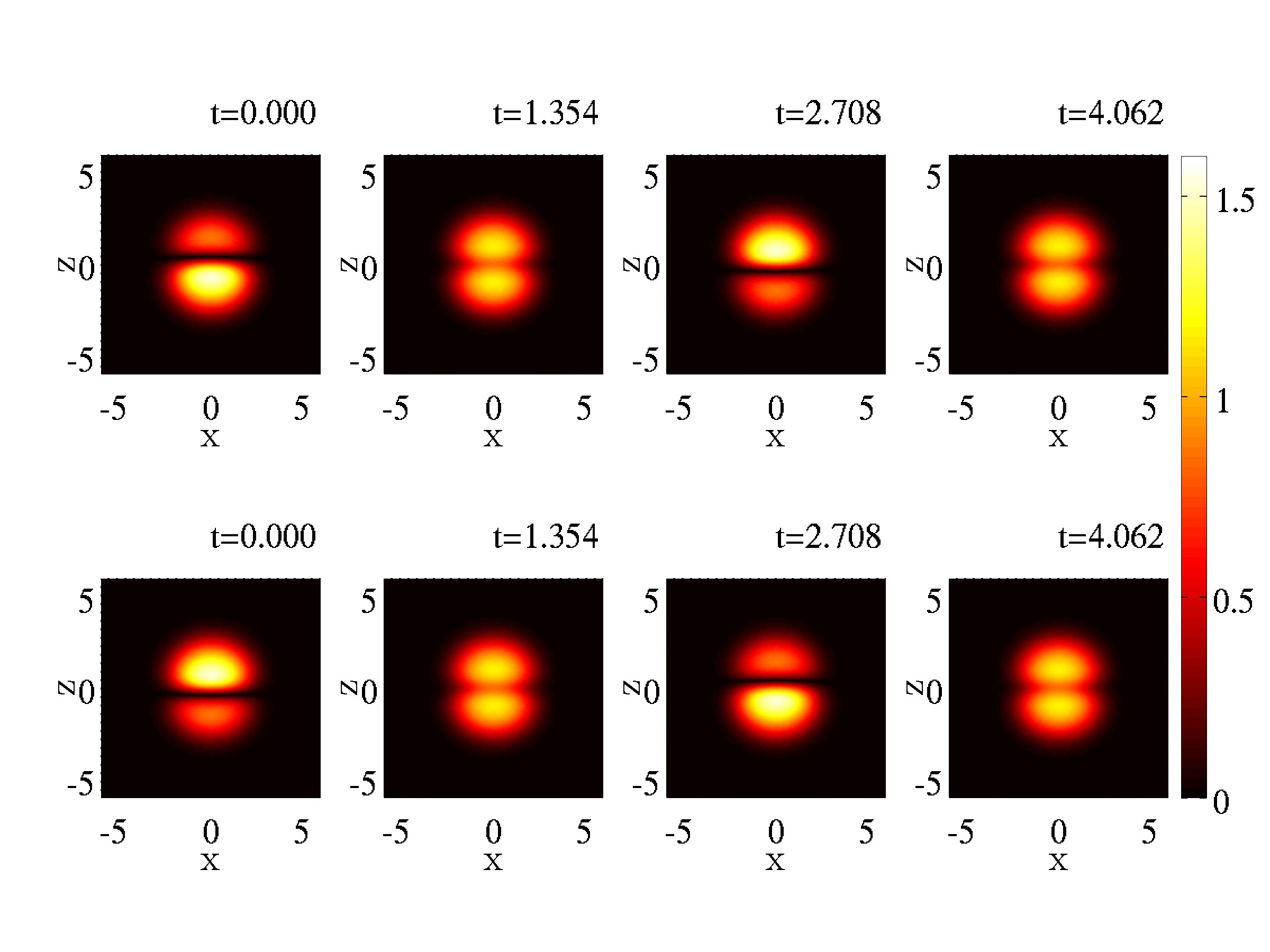
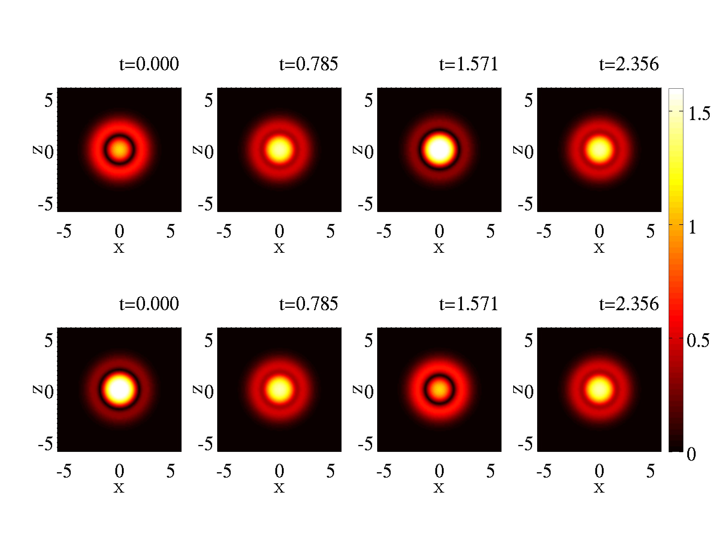
A complementary way to test this stability, but which also illustrates a different type of pattern that can emerge in two-component atomic BECs stems from the SO$(2)$ rotation-invariance of the Manakov model. In particular any pseudo-spinor state $(\psi_{1},\psi_{2})$ can be rotated by a unitary $2\times 2$ matrix (here we use simply an orthogonal rotation with an angle $\theta$), resulting still in an exact solution of the model. It is in this way that dark-dark solitons were obtained from dark-bright ones in 1d and this justified their relevance and spontaneous emergence in experiments pe4 ; pe5 . In the case of Fig. 3, we observe the stable oscillation patterns up to $t=100$ that result from the PDB (top) and SDB (bottom) cases. We have studied both symmetric and asymmetric mixing of the two components, and both are robust. Here we only show results of the symmetric case, i.e., $\theta=\pi/4$. Representative states at $t=0,\ T/4,\ T/2,\ 3T/4$, are shown where $T=2\pi/|\mu_{1}-\mu_{2}|$ is the oscillation period. It can be seen that the SO$(2)$ rotation of the PDB yields a novel state where there is a planar dark soliton in each component (one of which is at $z>0$ and one at $z<0$, with a complementary bright atomic mass in the other component). This can be dubbed a PDB-PDB state. Similarly the SDB-SDB state of the bottom two panels, resulting from the SO$(2)$ rotation of the SDB features an inner and an outer SDB state with the inner and outer dark shells residing in different components. See Ref. youtube for dynamical movies illustrating the details of the resulting oscillations.

Figure 1: (Color online) Top panels: Density profile of a representative three-dimensional dark-bright soliton at $\mu_{1}=12$ and $\mu_{2}=10$. Bottom panel: Spectrum of the dark-bright soliton along the line from the linear limit to $\mu_{1}=12$ and $\mu_{2}=10$. The red crosses and blue pluses are unstable and stable eigenvalues, respectively. The black and cyan lines are unstable and stable eigenvalues calculated using the degenerate perturbation theory. Note that they agree well near the linear limit, and the dark-bright soliton has a small interval where it is completely stable near but not including the linear limit.

Figure 2: (Color online) Top panels: Density profile of a representative three-dimensional dark-shell-bright soliton at $\mu_{1}=12$ and $\mu_{2}=10$. Bottom panel: Spectrum of the dark-shell-bright soliton along the line from the linear limit to $\mu_{1}=12$ and $\mu_{2}=10$. The red crosses and blue pluses are unstable and stable eigenvalues, respectively. The black and cyan lines are unstable and stable eigenvalues calculated using the degenerate perturbation theory. Note that they agree well near the linear limit, and the dark-shell-bright soliton is remarkably stable near the linear limit.

Figure 3: (Color online) Top two panels: Representative states of SO$(2)$ induced oscillation patterns at $t=0,\ T/4,\ T/2,\ 3T/4$ for $\mu_{1}=4.02$ and $\mu_{2}=2.86$ emerging from the rotation of the PDB. An oscillating pair of PDBs results. The oscillation period is $T=2\pi/(\mu_{1}-\mu_{2})\approx 5.4165$. The dynamics is in good agreement with the theoretical prediction, and is checked to be robust up to $t=100$, showing indirectly the stability of the dark-bright soliton at the chemical potentials studied. Bottom two panels: Same thing for the SO$(2)$ rotation of the SDB, resulting in a pair of SDBs oscillating one around the other. Here $\mu_{1}=4.86,\ \mu_{2}=2.86$, hence $T=\pi$.

III.2 Instability Dynamics for the PDB

We now turn to an examination of the unstable dynamics of the two states of interest in the regions of chemical potential where they become unstable. We can see that similarly to the one-component structures of russell (and dss for the SDBs), these states suffer a cascade of pitchfork bifurcations leading to the emergence of a sequence of unstable modes.

The first unstable mode of a planar dark soliton has been shown to lead to a 2 vortex line state; similarly, the unstable mode of a PDB in a two-component setting yields a 2 vortex line state trapping respective bright solitons i.e., a 2 vortex-line-bright (VLB) state. We have confirmed this by exploring the dynamics at $\mu_{1}=4.685,\ \mu_{2}=3.455$ up to $t=400$. The top panel of Fig. 4 shows the evolution of this instability and how the waveform departs from the PDB leading (upon its maximal deviation from it) to a 2 VLB state shown, a typical example of which is shown in the middle panel of the figure for $t=217$. However, then due to the recurrent dynamics of the Hamiltonian system, it returns to the PDB, oscillating back and forth between these two states over the time scale monitored. Nevertheless, it is interesting that each time the 2VLB soliton forms, it appears to forget its history and it possesses a different orientation in the $x\textrm{-}y$ plane.

Figure 4: (Color online) Top panel: The maximum densities of the two components in the $x\textrm{-}y$ plane in the dynamics of the PDB at $\mu_{1}=4.685,\ \mu_{2}=3.455$ up to $t=400$. The condensates oscillate between the PDB and the 2VLB soliton. Second row: Density profile of a 2VLB state at $t=217$ in the above PDB dynamics. Bottom two rows: Dynamics of PDB with the instability mode leading to a VRB at $\mu_{1}=6.015$, $\mu_{2}=4.645$.

In the case of a planar dark soliton, a second mode of instability (occurring very close to the emergence of the 2 VL state) leads to the bifurcation of a vortex ring (VR). Thus, we similarly expect that the second instability (after then one near $\mu_{1}\approx 4.3$ leading to 2 VLB) arising near $\mu_{1}\approx 4.8$ in Fig. 1 will lead to a vortex-ring-bright (VRB) solitonic state. To examine the outcome of this instability, we have monitored the dynamics at $\mu_{1}=6.015,\ \mu_{2}=4.645$ upto $t=200$. The VRB soliton was observed as shown in Fig. 4. We see that a VR is first formed, but the VR is unstable. It breaks through a quadrupolar ($n=2$) Kelvin mode to a 2VL. Subsequently, the 2VL come closer, exchange their segments and hence change to a new orientation. The 2VL then reconnects to form a highly excited VR. The VR is seen to break anew to 2VL, reconnect and break again. The subsequent dynamics of the 2VL are quite complex, and can oscillate within the trap. Note that the bright component changes its shape in tune with the vortex lines and rings of the first component.

III.3 Instability Dynamics for the SDB

Finally, we study the instability modes of the spherical dark bright solitary wave. Similarly to the case of the PDB, we turn to the analysis of the one-component state, in this case the dark soliton shell of dss for insights on the dynamical consequences of the modes of instability. We find there that the first mode of instability of the one-component state leads to a 6 vortex line “cage”, while the second one to a 6 vortex ring cage. We have thus followed the dynamics of our two-component SDB state at $\mu_{1}=6.9,\ \mu_{2}=4.9$ as shown in the top panel of Fig. 5 (for $t=79$). There, we observe indeed that the two-component analog of the 6 VL state, the 6 VLB is emerging through the unstable dynamics of the SDB. However, in turn, this state undergoes vortex line reconnections. For example, a pair of vertical vortex lines can exchange line segments and become horizontal. The 6VL cage is also observed to reappear, yet its dynamics leads to complex vortex line/ring dynamics and reconnections which we do not pursue further here.

Figure 5: (Color online) Top panel: Density profile of a 6VLB state at $t=79$, resulting from the unstable dynamics of a SDB soliton at $\mu_{1}=6.9,\ \mu_{2}=4.9$. Bottom two rows: Dynamics of SDB at $\mu_{1}=9.28,\ \mu_{2}=7.28$ leading through its instability mode to a 6VRB (the evolution is shown at different times).

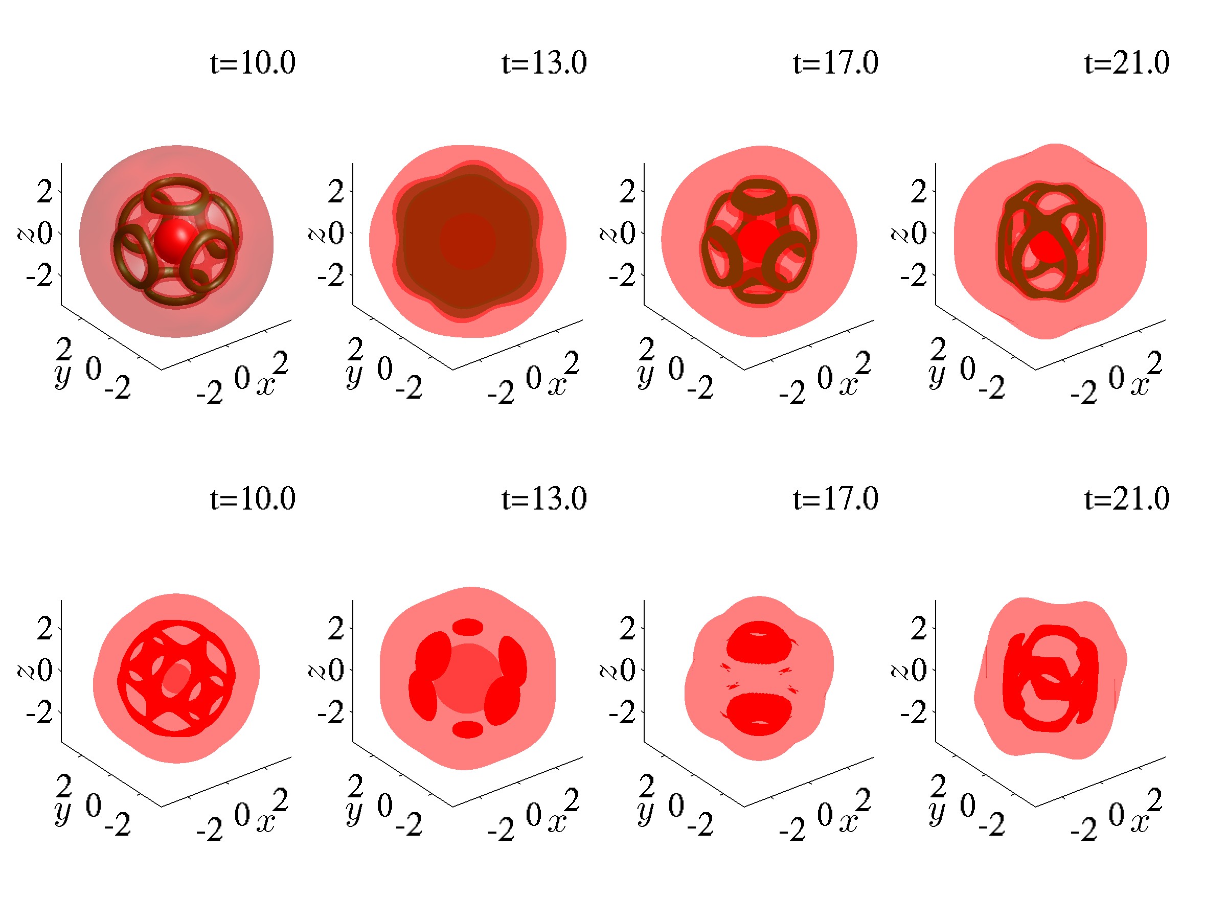
In line with the above discussion, the second unstable mode is expected to lead to a cage of vortex-ring-bright solitary waves (a 6 VRB state). We have performed dynamical simulations at $\mu_{1}=9.28,\ \mu_{2}=7.28$, and the 6 VRB cage is indeed observed around $t=10$ as shown in the bottom panels of Fig. 5. This state is more robust than the 6VLB cage, yet it is subsequently deformed for the chemical potentials studied. Nevertheless, we observe its recurrence, as well as the formation of more complex states involving VRBs in the relevant panels.

IV Conclusions and Future Challenges

In this work, we considered generalizations of the notion of the dark bright soliton in three-dimensional settings, including the planar dark bright solitary wave and the (spherical) shell dark-bright solitary wave. We constructed these structures systematically from the low density, linear limit of the mean-field model and continued them from there towards the high density, highly nonlinear limit of the system. Although we are well aware of the fact that for low densities, features such as quantum fluctuations carr will be important, nevertheless this limit is useful towards understanding how to systematically construct such states and how to assess their stability characteristics. In fact, in the vicinity of the linear limit, the developed (for the multi-component case) degenerate perturbation theory enables a systematic characterization of the different eigenmodes of the system. On the numerical side, we utilized the symmetry of the solutions to simplify the computation of the relevant eigenmodes which were found to be in good agreement with the theory. In the case of both the principal families considered, intervals of stability of the solutions were identified, although the states were found to be subject to symmetry breaking pitchfork bifurcations. The latter were numerically identified to lead to the emergence of vortex-line-bright and vortex-ring-bright solitary waves (and also multi-structure generalizations thereof). As an aside, we also explored SO$(2)$ rotations of the families considered, leading to pairs of planar and spherical dark bright states.

Our results lead to a number of interesting questions for future study. We can see from this work that vortex-line-bright solitons and vortex-ring-bright solitons and multi-solitons may spontaneously arise as a result of dynamical instabilities of other states. In that light, these entities merit independent study in their own right. The same is true for skyrmion states (consisting of a vortex ring coupled to a vortex line). The latter have been studied dynamically in earlier dynamical studies ruosteko , yet we propose a systematic analysis of their spectrum. It would be especially interesting to explore both for states such as the ones herein and for some of the above proposed extensions whether in the highly nonlinear limit a particle picture can be formulated describing the in-trap dynamics and multi-state interactions, as has been done earlier for vortices or vortex rings siambook . Such studies are presently in progress and will be reported in future publications.

APPENDIX A: LINEAR STABILITY CONSIDERATIONS

Linear stability analysis (Bogolyubov-de Gennes Analysis) shows that the stability is governed by the eigenvalues $\lambda$ of the following 4$\times$4 matrix $M$:

$$M_{11} = -i\left(-\frac{1}{2}\nabla^{2}+V-\mu_{1}+2|\psi^{0}_{1}|^{2}+|\psi^{0}_{2}|^{2}\right),$$

$$M_{12} = -i(\psi_{1}^{0})^{2},$$

$$M_{13} = -i\psi^{0}_{1}\psi_{2}^{0*},$$

$$M_{14} = -i\psi^{0}_{1}\psi^{0}_{2},$$

$$M_{21} = i(\psi_{1}^{0*})^{2},$$

$$M_{22} = i\left(-\frac{1}{2}\nabla^{2}+V-\mu_{1}+2|\psi^{0}_{1}|^{2}+|\psi^{0}_{2}|^{2}\right),$$

$$M_{23} = i\psi_{1}^{0*}\psi_{2}^{0*},$$

$$M_{24} = i\psi_{1}^{0*}\psi^{0}_{2},$$

$$M_{31} = -i\psi_{1}^{0*}\psi^{0}_{2},$$

$$M_{32} = -i\psi^{0}_{1}\psi^{0}_{2},$$

$$M_{33} = -i\left(-\frac{1}{2}\nabla^{2}+V-\mu_{2}+|\psi^{0}_{1}|^{2}+2|\psi^{0}_{2}|^{2}\right),$$

$$M_{34} = -i(\psi_{2}^{0})^{2},$$

$$M_{41} = i\psi_{1}^{0*}\psi_{2}^{0*},$$

$$M_{42} = i\psi^{0}_{1}\psi_{2}^{0*},$$

$$M_{43} = i(\psi_{2}^{0*})^{2},$$

$$M_{44} = i\left(-\frac{1}{2}\nabla^{2}+V-\mu_{2}+|\psi^{0}_{1}|^{2}+2|\psi^{0}_{2}|^{2}\right).$$ (11)

All the elements of the matrix aside from the diagonal ones are multiplicative, while $\psi_{1,2}^{0}$ denotes the (two components of the) stationary state around which the linearization is performed.

APPENDIX B: THE PARTIAL-WAVE METHOD

To compute the stability of stationary states away from the linear limit, we employ numerical computations. This is however very demanding in the full 3d setting. For stationary states with rotational symmetry up to a topological charge, the work can be significantly reduced by working in the $\rho\textrm{-}z$ plane. It is straightforward to compute the stationary states, taking advantage of the relevant symmetry. Here we present how to compute the stability for two-component solitons, generalizing the relevant discussion of Ref. dss for one-component solitons. Although we will utilize the method for the real PDB and SDB profiles in $\psi_{1}^{0}$ and $\psi_{2}^{0}$, we present the (partial-wave) method for the stability in a more general form.

The Laplacian in the cylindrical coordinates $(\rho,\phi,z)$ is decomposed as follows:

$$\nabla^{2}f=\Delta_{H}f+\frac{\Delta_{G}f}{\rho^{2}},$$ (12)

where its components read:

$$\Delta_{H}f = \frac{1}{\rho}\frac{\partial}{\partial\rho}\left(\rho\frac{\partial f}{\partial\rho}\right)+\frac{\partial^{2}f}{\partial z^{2}},$$ (13)

$$\Delta_{G}f = \frac{\partial^{2}f}{\partial\phi^{2}}.$$ (14)

For states with rotational symmetry with topological charges $S_{1}$ and $S_{2}$, we have

$$\psi^{0}_{1}(\vec{r}) = \psi^{0}_{1}(\rho,z)e^{iS_{1}\phi}$$

$$\psi^{0}_{2}(\vec{r}) = \psi^{0}_{2}(\rho,z)e^{iS_{2}\phi},$$ (15)

and Eqs. (II.1) become:

$$-\frac{1}{2}\Delta_{H}\psi^{0}_{1}+\frac{S_{1}^{2}}{2\rho^{2}}\psi^{0}_{1}+V\psi^{0}_{1}+(|\psi^{0}_{1}|^{2}+|\psi^{0}_{2}|^{2})\psi^{0}_{1} = \mu_{1}\psi^{0}_{1}$$

$$-\frac{1}{2}\Delta_{H}\psi^{0}_{2}+\frac{S_{2}^{2}}{2\rho^{2}}\psi^{0}_{2}+V\psi^{0}_{2}+(|\psi^{0}_{1}|^{2}+|\psi^{0}_{2}|^{2})\psi^{0}_{2} = \mu_{2}\psi^{0}_{2}.$$

For a generic perturbation, using Fourier analysis,

$$\psi_{1} = e^{iS_{1}\phi}\left[\psi^{0}_{1}+\delta\sum\limits_{m}\left[a_{m}(\rho,z,t)e^{im\phi}+c_{m}^{*}(\rho,z,t)e^{-im\phi}\right]\right]$$

$$\psi_{2} = e^{iS_{2}\phi}\left[\psi^{0}_{2}+\delta\sum\limits_{m}\left[b_{m}(\rho,z,t)e^{im\phi}+d_{m}^{*}(\rho,z,t)e^{-im\phi}\right]\right],$$

Substituting this expansion into the GPE, keeping the terms to O$(\delta)$ of the perturbations and using the uniqueness of the Fourier series of both sides, one can get for each mode $m$:

$$i\dot{a}_{m} = -\frac{1}{2}\Delta_{H}a_{m}+\frac{(m+S_{1})^{2}}{2\rho^{2}}a_{m}+Va_{m}-\mu_{1}a_{m}$$

$$+ (2|\psi^{0}_{1}|^{2}+|\psi^{0}_{2}|^{2})a_{m}+\psi^{0}_{1}\psi_{2}^{0*}b_{m}+\psi_{1}^{02}c_{m}+\psi^{0}_{1}\psi^{0}_{2}d_{m}$$

$$i\dot{c}_{m}^{*} = -\frac{1}{2}\Delta_{H}c_{m}^{*}+\frac{(m-S_{1})^{2}}{2\rho^{2}}c_{m}^{*}+Vc_{m}^{*}-\mu_{1}c_{m}^{*}$$

$$+ (2|\psi^{0}_{1}|^{2}+|\psi^{0}_{2}|^{2})c_{m}^{*}+\psi_{1}^{02}a_{m}^{*}+\psi^{0}_{1}\psi^{0}_{2}b_{m}^{*}+\psi^{0}_{1}\psi_{2}^{0*}d_{m}^{*}$$

$$i\dot{b}_{m} = -\frac{1}{2}\Delta_{H}b_{m}+\frac{(m+S_{2})^{2}}{2\rho^{2}}b_{m}+Vb_{m}-\mu_{2}b_{m}$$

$$+ (|\psi^{0}_{1}|^{2}+2|\psi^{0}_{2}|^{2})b_{m}+\psi_{1}^{0*}\psi^{0}_{2}a_{m}+\psi^{0}_{1}\psi^{0}_{2}c_{m}+\psi_{2}^{02}d_{m}$$

$$i\dot{d}_{m}^{*} = -\frac{1}{2}\Delta_{H}d_{m}^{*}+\frac{(m-S_{2})^{2}}{2\rho^{2}}d_{m}^{*}+Vd_{m}^{*}-\mu_{2}d_{m}^{*}$$

$$+ (|\psi^{0}_{1}|^{2}+2|\psi^{0}_{2}|^{2})d_{m}^{*}+\psi^{0}_{1}\psi^{0}_{2}a_{m}^{*}+\psi_{2}^{02}b_{m}^{*}+\psi_{1}^{0*}\psi_{2}^{0}c_{m}^{*}.$$

Normal modes of the form $(a_{m}(t),c_{m}(t),b_{m}(t),d_{m}(t))^{T}=(a_{m}(0),c_{m}(0),b_{m}(0),d_{m}(0))^{T}\exp(\lambda t)$ lead to the following eigenvalue problems of the 4$\times$4 matrix $M$, with eigenvalues $\lambda$:

$$M_{11} = i\left(\frac{1}{2}\Delta_{H}-\frac{(m+S_{1})^{2}}{2\rho^{2}}-V+\mu_{1}-2|\psi^{0}_{1}|^{2}-|\psi^{0}_{2}|^{2}\right),$$

$$M_{12} = -i(\psi_{1}^{0})^{2},$$

$$M_{13} = -i\psi^{0}_{1}\psi_{2}^{0*},$$

$$M_{14} = -i\psi^{0}_{1}\psi^{0}_{2},$$

$$M_{21} = i(\psi_{1}^{0*})^{2},$$

$$M_{22} = i\left(-\frac{1}{2}\Delta_{H}+\frac{(m-S_{1})^{2}}{2\rho^{2}}+V-\mu_{1}+2|\psi^{0}_{1}|^{2}+|\psi^{0}_{2}|^{2}\right),$$

$$M_{23} = i\psi_{1}^{0*}\psi_{2}^{0*},$$

$$M_{24} = i\psi_{1}^{0*}\psi^{0}_{2},$$

$$M_{31} = -i\psi_{1}^{0*}\psi^{0}_{2},$$

$$M_{32} = -i\psi^{0}_{1}\psi^{0}_{2},$$

$$M_{33} = -i\left(-\frac{1}{2}\Delta_{H}+\frac{(m+S_{2})^{2}}{2\rho^{2}}+V-\mu_{2}+|\psi^{0}_{1}|^{2}+2|\psi^{0}_{2}|^{2}\right),$$

$$M_{34} = -i(\psi_{2}^{0})^{2},$$

$$M_{41} = i\psi_{1}^{0*}\psi_{2}^{0*},$$

$$M_{42} = i\psi^{0}_{1}\psi_{2}^{0*},$$

$$M_{43} = i(\psi_{2}^{0*})^{2},$$

$$M_{44} = i\left(-\frac{1}{2}\Delta_{H}+\frac{(m-S_{2})^{2}}{2\rho^{2}}+V-\mu_{2}+|\psi^{0}_{1}|^{2}+2|\psi^{0}_{2}|^{2}\right).$$

One can prove using an orthogonal transformation and the symmetry of the $M$ matrix that the eigenvalues of the mode $-m$ are complex conjugates of the mode $m$, therefore, one only needs to compute eigenvalues of the non-negative $m$ modes. In the following calculations, we use $m=0,1,2,...,5$ as in Ref. dss . We apply the methods to the planar dark bright (PDB) and the spherical dark bright (SDB) solitary waves in this work. Note that the method works for a large class of solitons that are of interest including but not limited to the vortex-line-bright, vortex-ring-bright stathis and the skyrmion states ruosteko .

References

- (1) Yu.S. Kivshar and G.P. Agrawal, Optical solitons: from fibers to photonic crystals, Academic Press (San Diego, 2003).
- (2) L.P. Pitaevskii and S. Stringari, Bose-Einstein Condensation, Oxford University Press (Oxford, 2003).
- (3) P. G. Kevrekidis and D. J. Frantzeskakis, Rev. Phys. 1, 140 (2016).
- (4) S. V. Manakov, Sov. Phys. JETP, 38, 248–253 (1973).
- (5) V. E. Zakharov and S. V. Manakov, Sov. Phys. JETP, 42, 842–850 (1976).
- (6) M. J. Ablowitz, B. Prinari, and A. D. Trubatch, Discrete and Continuous Nonlinear Schrödinger Systems, Cambridge University Press (Cambridge, 2004).
- (7) P. G. Kevrekidis, D. J. Frantzeskakis, and R. Carretero-González, The Defocusing Nonlinear Schrödinger Equation, SIAM (Philadelphia, 2015).
- (8) Z. Chen, M. Segev, T. H. Coskun, D. N. Christodoulides, and Yu. S. Kivshar, J. Opt. Soc. Am. B, 14, 3066–3077 (1997).
- (9) E. A. Ostrovskaya, Yu. S. Kivshar, Z. Chen, and M. Segev, Opt. Lett., 24, 327–329 (1999).
- (10) Th. Busch and J. R. Anglin, Phys. Rev. Lett., 87, 010401 (2001).
- (11) C. Becker, S. Stellmer, P. Soltan-Panahi, S. Dörscher, M. Baumert, E.-M. Richter, J. Kronjäger, K. Bongs, and K. Sengstock, Nature Phys., 4, 496–501 (2008).
- (12) C. Hamner, J. J. Chang, P. Engels, and M. A. Hoefer, Phys. Rev. Lett., 106, 065302 (2011).
- (13) S. Middelkamp, J. J. Chang, C. Hamner, R. Carretero-González, P. G. Kevrekidis, V. Achilleos, D. J. Frantzeskakis, P. Schmelcher,and P. Engels, Phys. Lett. A, 375, 642–646 (2011).
- (14) D. Yan, J. J. Chang, C. Hamner, P. G. Kevrekidis, P. Engels, V. Achilleos, D. J. Frantzeskakis, R. Carretero-González, and P. Schmelcher, Phys. Rev. A, 84, 053630 (2011).
- (15) M. A. Hoefer, J. J. Chang, C. Hamner, and P. Engels, Phys. Rev. A, 84, 041605(R) (2011).
- (16) D. Yan, J. J. Chang, C. Hamner, M. Hoefer, P. G. Kevrekidis, P. Engels, V. Achilleos, D. J. Frantzeskakis, and J. Cuevas, J. Phys. B: At. Mol. Opt. Phys., 45, 115301 (2012).
- (17) A. Álvarez, J. Cuevas, F. R. Romero, C. Hamner, J. J. Chang, P. Engels, P. G. Kevrekidis, and D. J. Frantzeskakis, J. Phys. B, 46, 065302 (2013).
- (18) G. C. Katsimiga, J. Stockhofe, P. G. Kevrekidis, P. Schmelcher, arXiv:1611.04915.
- (19) D. N. Christodoulides, Phys. Lett. A, 132, 451–452 (1988).
- (20) V. V. Afanasyev, Yu. S. Kivshar, V. V. Konotop, and V. N. Serkin, Opt. Lett., 14, 805–807 (1989).
- (21) Yu. S. Kivshar and S. K. Turitsyn, Opt. Lett., 18, 337–339 (1993).
- (22) R. Radhakrishnan and M. Lakshmanan, J. Phys. A: Math. Gen., 28, 2683–2692 (1995).
- (23) A. V. Buryak, Yu. S. Kivshar, and D. F. Parker, Phys. Lett. A, 215, 57–62 (1996).
- (24) A. P. Sheppard and Yu. S. Kivshar, Phys. Rev. E, 55, 4773–4782 (1997).
- (25) Q.-H. Park and H. J. Shin, Phys. Rev. E, 61, 3093–3106 (2000).
- (26) W. Wang, P. G. Kevrekidis, R. Carretero-González, and D. J. Frantzeskakis Phys. Rev. A 93, 023630 (2016).
- (27) E. G. Charalampidis, W. Wang, P. G. Kevrekidis, D. J. Frantzeskakis, and J. Cuevas-Maraver Phys. Rev. A 93, 063623 (2016).
- (28) P. G. Kevrekidis, D. J. Frantzeskakis, and R. Carretero-González (eds.), Emergent Nonlinear Phenomena in Bose-Einstein Condensates. Theory and Experiment (Springer-Verlag, Berlin, 2008);
- (29) It is worthwhile to mention that the precise value of the coefficients is still under active investigation, with the most accurate values known presently being those of M. Egorov, B. Opanchuk, P. Drummond, B. V. Hall, P. Hannaford, and A. I. Sidorov, Phys. Rev. A 87, 053614 (2013).
- (30) R. N. Bisset, Wenlong Wang, C. Ticknor, R. Carretero-González, D. J. Frantzeskakis, L. A. Collins, and P. G. Kevrekidis Phys. Rev. A 92, 043601 (2015).
- (31) See for relevant movies: https://www.youtube.com/watch?v=dKyuGrw4stw and https://www.youtube.com/watch?v=EOWnYHDPiPQ
- (32) J. Ruostekoski and J. R. Anglin Phys. Rev. Lett. 86, 3934 (2001); C. M. Savage and J. Ruostekoski Phys. Rev. Lett. 91, 010403 (2003).
- (33) L. D. Carr (Ed.), Understanding Quantum Phase Transitions, Taylor and Francis (Boca Raton, 2010)