Synthetic gauge potential and effective magnetic field in a Raman medium undergoing molecular modulation

Abstract

We theoretically demonstrate non-trivial topological effects for a probe field in a Raman medium undergoing molecular modulation processes. The medium is driven by two non-collinear pump beams. We show that the angle between the pumps is related to an effective gauge potential and an effective magnetic field for the probe field in the synthetic space consisting of a synthetic frequency dimension and a spatial dimension. As a result of such effective magnetic field, the probe field can exhibit topologically-protected one-way edge state in the synthetic space, as well as Landau levels which manifests as suppression of both diffraction and sideband generation. Our work identifies a previously unexplored route towards creating topological photonics effects, and highlights an important connection between topological photonics and nonlinear optics.

The process of molecular modulation (Fig. 1(a)) has attracted significant interests in the last two decades boyd ; harris98 ; sokolov00 ; sokolov ; yzvuz03 ; huang06 ; yzvuz07 ; suzuki08 ; wang10 . In this process, molecules are driven by two pump fields, which generate coherence between a few low-lying vibrational/rotational levels through a Raman transition. A probe field couples with the molecular coherence, which results in the generation of Raman sidebands. This process is highly efficient and has found applications in attosecond pulse generation baker11 , coherent broadband light generation zhi07 ; wang14 , and optical orbital angular momentum transfer strohaber12 ; strohaber15 .

Most previous experiments on molecular modulation assumes a collinear propagation between the pump and the probe (Fig. 1(b)). In this Letter, we consider a pump configuration as shown in Fig. 1(c), where two pump beams are assumed to be non-collinear, with both their directions near the $z$-axis, subtending an angle $\alpha\ll 1$ rad. We show that when a probe beam propagating along the $z$-axis is introduced into this medium, such a molecular coherence results in a synthetic gauge field that couples to the probe field. As a result the probe field exhibits non-trivial topological photonic effect including a topologically protected one-way edge state along the frequency axis, as well as Landau levels which manifests as suppression of both diffraction and sideband generation.

The explorations of synthetic gauge potential hafezi11 ; umucalilar11 ; fang12prln ; fang12np ; rechstman12 ; tzuang14n ; li14n ; fu15 and topological effects raghu08 ; haldane08 ; wang08 ; khanikaev13 ; rechstman13 ; hafezi13 ; mittal14 ; lu14 ; celi14 ; luo14 ; wang15 for light have generated significant recent interests since these effects open a new dimension in the control of the flow of light. Most previous works on synthetic gauge field and topological photonics rely upon complex material geometries. In contrast, in this work we show that topological photonic effects naturally arise in a standard nonlinear optics geometry. Our work therefore points to a potentially fruitful direction at the interface between nonlinear optics and topological photonics. The predicted effects also represent a new mechanism for controlling Raman sidebands in system exhibiting molecular coherence.

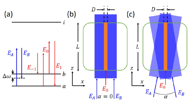
Figure 1: (a) Energy levels of a molecule used in the molecular modulation process. Levels $a$ and $b$ are ground states and $i$ are the excited states. Pump fields $E_{A}$ and $E_{B}$ are far from resonance between the ground states and the excited states, but are near resonance with the two-photon transition $a$-$b$. Sidebands $E_{n}$ are generated via the interaction of molecular coherence $\rho_{ab}$ as generated from the pump, with the probe field $E_{0}$. (b) and (c) Pump fields and the probe field are injected into the Raman-active medium (inside a cell in the green square with a length $L$) along near the $z$-direction. Two pump fields (blue regions) propagate collinearly at an angle $\alpha=0$ in (b) or non-collinearly at $\alpha=0.5^{\circ}$ in (c). The probe field (red arrow) has a focal area at $z=0$ which is much smaller than the beam waist of the pump fields. The simulation region has a width $D$ and is labelled in orange.

We start our analysis by considering a molecular Raman-active medium. The molecules have a ground state (labelled as “$a$” in Fig. 1(a)), a low-lying excited (labelled as “$b$”), and intermediate states (labelled as “$i$”) at higher energies. The medium is driven by two pump laser pulses, centered at frequencies $\omega_{A}$ and $\omega_{B}$, respectively. The pumps are non-resonant with respect to any molecular transitions but are two-photon near-resonant with the $a$-$b$ transition with a small detuning $\Delta\omega\equiv(\omega_{b}-\omega_{a})-(\omega_{A}-\omega_{B})$. The pumps create a coherence $\rho_{ab}$ between levels $a$ and $b$, which can generate sidebands for the pump fields themselves sokolov . However, we emphasize here that we are not interested in this sideband generation. Instead we send a weak probe field $E_{0}$ into the medium. To distinguish the different sidebands from the probe and from the pumps, one can send the probe either as a short pulse that arrives at a time delay after the short pump pulses have passed through the medium, or at a very different frequency from the pump fields while the pumps stay in the medium. In both cases, the key physics for our purpose here is the interaction of the pump fields with the coherence generated by the pumps. Therefore, we adopt the analytic model as was used in harris98 ; sokolov ; sokolov02 , where both the pumps and the probe are treated as continuous-wave at a single frequency, and we provide an estimate on the effects of the pulses towards the end of the paper.

The propagation equation of a laser beam at a frequency $\omega$ is derived from the Maxwell’s equations as sokolov ; sokolov02 :

$$\frac{\partial}{\partial z}E_{\omega}-i\frac{c}{2\omega}\frac{\partial^{2}}{\partial x^{2}}E_{\omega}=ic\mu_{0}\hbar\omega P_{\omega}.$$ (1)

Here, we assume the beam has a propagation direction near the $z$-axis and use the paraxial wave approximation. $\mu_{0}$ is the vacuum permeability, and $E_{\omega}$ and $P_{\omega}$ are the slowly varying envelopes for the spectral components of the electric field and the polarization, respectively, at the frequency $\omega$.

For the pumps $E_{A(B)}$, we use the solution of $P_{\omega}$ in Refs. harris98 ; sokolov ; sokolov02 and write Eq. (1) as

$$\frac{\partial}{\partial z}E_{A(B)}-i\frac{c}{2\omega_{A(B)}}\frac{\partial^{2}}{\partial x^{2}}E_{A(B)}=ic\mu_{0}\hbar\omega_{A(B)}N\left[a_{\omega_{A(B)}}\rho_{aa}+d_{\omega_{A(B)}}\rho_{bb}\right]E_{A(B)},$$ (2)

where $N$ is the number density of the molecule. In Eq. (2),

$$a_{\omega}=\frac{1}{2\hbar^{2}}\sum_{i}\left[\frac{|\mu_{ai}|^{2}}{(\omega_{i}-\omega_{a})-\omega}+\frac{|\mu_{ai}|^{2}}{(\omega_{i}-\omega_{a})+\omega}\right],$$ (3)

$$d_{\omega}=\frac{1}{2\hbar^{2}}\sum_{i}\left[\frac{|\mu_{bi}|^{2}}{(\omega_{i}-\omega_{b})-\omega}+\frac{|\mu_{bi}|^{2}}{(\omega_{i}-\omega_{b})+\omega}\right],$$ (4)

where $\mu_{a(b)i}$ is the dipole moment between levels $a(b)$ and intermediate state $i$. In Eq. (2) we only keep the first-order perturbation to the pumps because we are interested in the sideband generation from the probe. Because the pumps are non-resonant with respect to any molecular transition, we have $a_{\omega_{A(B)}}\cong d_{\omega_{A(B)}}\cong a_{0}$. By using $\rho_{aa}+\rho_{bb}=1$, Eqs. (2) becomes

$$i\frac{\partial}{\partial z}E_{A(B)}=-\kappa_{A(B)}\frac{\partial^{2}}{\partial x^{2}}E_{A(B)}-\beta_{A(B)}E_{A(B)},$$ (5)

where $\kappa_{A(B)}=c/2\omega_{A(B)}$, and

$$\beta_{A(B)}=c\mu_{0}\hbar\omega_{A(B)}Na_{0}.$$ (6)

Therefore, the pump fields in general can be described as a Gaussian or Hermite-Gaussian beam with the wave vector $k_{A(B)}+\beta_{A(B)}$.

The pumps create coherence $\rho_{ab}$ between levels $a$ and $b$, which oscillates at the frequency $\omega_{m}=\omega_{A}-\omega_{B}$ (see Fig. 1(a)) with an amplitude of harris98 ; sokolov ; sokolov02 :

$$\rho_{ab}=\frac{1}{2}\frac{b_{\omega_{A}}E_{A}E_{B}^{*}}{\sqrt{|b_{\omega_{A}}E_{A}E_{B}^{*}|^{2}+\Delta\omega^{2}}},$$ (7)

where

$$b_{\omega}=\frac{1}{2\hbar^{2}}\sum_{i}\left[\frac{\mu_{ai}\mu_{bi}^{*}}{(\omega_{i}-\omega_{a})-\omega}+\frac{\mu_{ai}\mu_{bi}^{*}}{(\omega_{i}-\omega_{b})+\omega}\right].$$ (8)

To study the propagation of the probe, based on the experimental scenarios as described above, we assume that the coherence does not decay as the weak probe field propagates through the medium. The probe has the carrier frequency $\omega_{0}$. When the probe interacts with the coherence in the medium, sidebands at frequencies $\omega_{n}=\omega_{0}+n\omega_{m}$ are generated, where $n$ is an integer. From Eq. (1). the propagation equation for the electric field in the $n$-th sideband $E_{n}$ is harris98 ; sokolov ; sokolov02

$$\frac{\partial}{\partial z}E_{n}-i\frac{c}{2\omega_{n}}\frac{\partial^{2}}{\partial x^{2}}E_{n}=ic\mu_{0}\hbar\omega_{n}N\left\{\left[a_{\omega_{n}}\rho_{aa}+d_{\omega_{n}}\rho_{bb}\right]E_{n}+b^{*}_{\omega_{n}}\rho_{ab}E_{n-1}+b_{\omega_{n+1}}\rho_{ab}^{*}E_{n+1}\right\},$$ (9)

where $a_{\omega}$ and $d_{\omega}$ are defined in Eqs. (3) and (4), and $b_{\omega}$ is defined in Eq. (8). Since all the sidebands are sufficiently far from any resonance, again we have

$${\begin{array}[]{*{20}c}a_{\omega_{n}}\cong d_{\omega_{n}}\cong a_{0};&b_{\omega_{n}}\cong b_{0}\\ \end{array}}.$$ (10)

Therefore, Eq. (9) simplifies to

$$i\frac{\partial}{\partial z}E_{n}=\beta_{n}E_{n}-\kappa_{n}\frac{\partial^{2}}{\partial x^{2}}E_{n}-g_{n}\left(2\rho_{ab}E_{n-1}+2\rho_{ab}^{*}E_{n+1}\right),$$ (11)

where $\kappa_{n}=c/2\omega_{n}$, $\beta_{n}=c\mu_{0}\hbar\omega_{n}Na_{0}$, and $g_{n}=c\mu_{0}\hbar\omega_{n}Nb_{0}/2$.

From Eq. (7), with the pump configuration as described in Fig. 1(c), we have

$$\rho_{ab}(x,z)=\frac{1}{2}\frac{|b_{\omega_{A}}E_{A}(x)E_{B}^{*}(x)|}{\sqrt{|b_{\omega_{A}}E_{A}(x)E_{B}^{*}(x)|^{2}+\Delta\omega^{2}}}e^{i\theta(x)}e^{-i(\beta_{A}-\beta_{B})z},$$ (12)

where

$$\theta(x)=qx,$$ (13)

with $q\approx\alpha(k_{A}+k_{B})/2$. On the other hand, from Eq. (6), one can show that $\beta_{n}-\beta_{n-1}=\beta_{m}=\beta_{A}-\beta_{B}$. Therefore, we perform the transformation $E_{n}=\tilde{E}_{n}\exp(i\beta_{n}z)$ and $\rho_{ab}=\tilde{\rho}_{ab}\exp(i\beta_{m}z)$ to obtain

$$i\frac{\partial}{\partial z}\tilde{E}_{n}=-\kappa\frac{\partial^{2}}{\partial x^{2}}\tilde{E}_{n}-g(x)\left(e^{iqx}\tilde{E}_{n-1}+e^{-iqx}\tilde{E}_{n+1}\right).$$ (14)

In arriving at Eq. (14), we note that in the limit of $\omega_{0}\gg\omega_{m}$, $\kappa_{n}\cong\kappa$ and $2g_{n}|\rho_{ab}|\cong g$ supple .

To understand the physics in Eq. (14), we apply a gauge transformation $\tilde{E}_{n}=\varepsilon_{n}e^{inqx}$, define a continuous function $\varepsilon(\omega,x)$ such that $\varepsilon(\omega_{n},x)=\varepsilon_{n}$, and approximate the term in the parentheses by a continuous derivative. Eq. (14) becomes

$$i\frac{\partial}{\partial z}\varepsilon(\omega,x)\approx\kappa\left(-i\frac{\partial}{\partial x}+\frac{\omega-\omega_{0}}{\omega_{m}}q\right)^{2}\varepsilon(\omega,x)+g\omega_{m}^{2}\left(-i\frac{\partial}{\partial\omega}\right)^{2}\varepsilon(\omega,x)-2g\varepsilon(\omega,x).$$ (15)

Eq. (15) has the form of a Schrödinger equation in $2+1$ dimensions, except with the usual time axis replaced by the $z$-axis, and with the remaining two dimensions describing a synthetic space with one spatial dimension along the $x$ direction and one synthetic frequency dimension yuanOL ; ozawa16 . In this synthetic space, Eq. (15) describes an effective gauge potential $A_{\omega}=(\omega-\omega_{0})q/\omega_{m}$ along the $x$-axis, which gives a uniform effective magnetic field orthogonal to the 2D space:

$$B=\frac{\partial A}{\partial\omega}=\frac{q}{\omega_{m}}=\alpha\frac{(k_{A}+k_{B})}{2\omega_{m}}.$$ (16)

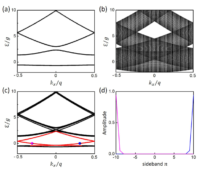
Figure 2: (a) The projected bandstructure within the first Brillouin zone $k_{x}\in[-q/2,q/2]$ in a infinite system described by Eq. (14). We choose $\kappa=g(\pi/2q)^{2}$. (b) The projected bandstructure with $q=0$ but with $\kappa$ unchanged plotted in the same first Brillouin zone. (c) The projected bandstructure in a 2D strip that is infinite along the $x$-axis but with a finite number of sidebands (sideband number $n=-10,\ldots,10$) along the frequency dimension. In the lowest bandgap, there exists two one-way edge modes (labelled in red). (d) Field amplitudes of the two edge modes labelled by purple and blue dots in (c).

To examine the topological effect created by such an effective magnetic field, we calculate the bandstructure of an infinite 2D system described by Eq. (14) with a uniform $g(x)=g$ along the $x$-direction. Eq. (14) has a spatial periodicity of $2\pi/q$ along the $x$-axis as well as a symmetry with respect to the translational operation $n$ to $n+1$ along the frequency axis. Therefore, it can be described in terms of a bandstructure $\mathcal{E}(k_{x},k_{\omega})$, which relates the wavevector shift for the probe $\mathcal{E}$ along the $z$-direction, to the quantum numbers $k_{x}$ and $k_{\omega}$ corresponding to the translational symmetries as described above. We take $\kappa=g(\pi/2q)^{2}$ and plot the projected bandstructure within the first Brillouin zone $k_{x}\in[-q/2,q/2]$ in Fig. 2(a). Due to the effective magnetic field, for each $k_{x}$ the bands are almost completely flat along the $k_{\omega}$ axis. Therefore, the projected bands appear as lines in the $\mathcal{E}-k_{x}$ plane. The bulk bands here correspond to the Landau level of a particle under a constant magnetic field. In the continuum limit (such as described by Eq. (15)) the bands would be completely flat along both the $k_{x}$ and the $k_{\omega}$ axis. Here the non-zero slope along the $k_{x}$ axis arises from the discrete translational symmetry. There are gaps between the bands. In contrast, with $q=0$, which corresponds to the use of two collinear pump beams, we observe neither the Landau level formation nor the opening of the band gaps in the projected bandstructure (Fig. 2(b)).

The bands in Fig. 2(a) are topologically non-trivial as characterized by non-zero Chern numbers tkkn . Therefore, in a strip geometry there should be topologically protected one-way edge states within the gap. As a demonstration, we consider a strip that is infinite along the $x$-axis but with finite numbers of $n$ ($n=-10,\ldots,10$) along the frequency axis. We plot its bandstructure $\mathcal{E}(k_{x})$ in Fig. 2(c). In the lowest bandgap, there exists two one-way edge modes. The field amplitudes corresponding to the two modes at $\mathcal{E}=0$ (labelled by purple and blue dots in Fig. 2(c)) are shown in Fig. 2(d). One can see that the fields are located on the two edges and decay exponentially into the bulk. The bandstructure analysis here indeed shows the non-trivial topology when the pumps are non-collinear.

While topological effects have been observed in a wide variety of photonic systems, the process of molecular modulation provides unique aspect of probing topological effects. To illustrate these effects, in what follows we will solve Eq. (14) numerically for several different pump and probe configurations. The parameters used in our simulations are based on the recent experiments in either the gas medium sokolov00 ; sokolov ; huang06 or the Raman-active crystal zhi07 ; wang14 . The molecular density is chosen to be $N\sim 10^{18}$-$10^{19}$ cm^-3. The frequencies of the pump and probe lasers are at the order of 1 $\mathrm{\mu m}$. Given these conditions, we have $g\sim 10^{2}$-$10^{3}$ m^-1, $\kappa\sim 10^{-7}$ m. At $z=0$, the probe field has a spatial profile of

$$f(x)=e^{-(x/\Delta x)^{2}},$$ (17)

with a focal width $\Delta x=38.8$ $\mathrm{\mu}$m. We will study the propagation of this probe field along the $z$-axis.

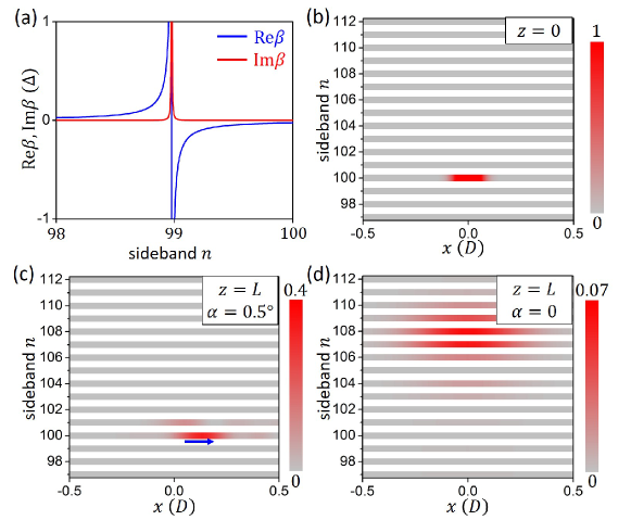
Figure 3: (a) The wave vector mismatching for the probe along $z$-direction, $\beta(\omega_{n})$, with an additional two-level atom added into the medium at a resonant frequency $\omega_{99}-0.025\omega_{m}$. $\Delta=10^{3}$ m^-1. (b) The normalized intensity as a function of position and sidebands for the input probe field. The input field has a frequency of $100.8\omega_{m}$. (c) and (d) The output field intensity at $z=L$, corresponding to the non-collinear pump geometry in Fig. 1(c) and the collinear pump geometry in Fig. 1(b). Blue arrow in (c) indicates the propagation direction of the edge state.

In Fig. 3 we present the simulation results for the system with a non-collinear pump geometry with $\alpha=0.5^{\circ}$, which gives $q=5\times 10^{4}$ m^-1. We choose $\kappa\sim 10^{-7}$ m, and $g=10^{2}$ m^-1. These parameters are the same as used for generating the bandstructure in Fig. 2(c). The beam waists of the pump fields are chosen to be $w_{0}=1$ mm which corresponds to the Rayleigh length $z_{R}\sim 3$ m. The length of the medium is $L=5$ cm. We perform the simulation in a $D\times L$ region as represented by the orange rectangle in Fig. 1(c), with $D=0.433$ mm, because the probe field doesn’t diffract out of this region in the entire simulation. Since $D<w_{0}$ and $L\ll z_{R}$, we assume that the amplitudes of the pump fields is uniform in the simulation region so the coherence is also uniform along $x$-direction in Eq. (14). In order to create an edge along the frequency axis, we add two-level atoms into the system that provides additional frequency dispersion. We choose two-level atoms to have a resonant frequency $\omega_{99}-0.025\omega_{m}$, a density of $2.5\times 10^{15}$ cm^-3, and a dephasing rate $1/T_{2}=10^{10}/2\pi$ s^-1. Here $\omega_{99}$ is the frequency of the $99^{\mathrm{th}}$ sideband, and the $n$-th sideband frequency satisfies $\omega_{n}=(n+0.8)\omega_{m}$. The wavevector $\beta$ as a function of frequency near the resonant frequency of the two-level atoms is shown in Fig. 3(a). Such two-level atoms strongly influence the wavevectors at the $99^{\mathrm{th}}$ sideband without influencing the wavevector of $100^{\mathrm{th}}$ sideband. With such a choice we expect that the $100^{\mathrm{th}}$ sideband cannot downconvert, which creates a boundary along the frequency axis. In the simulation, we input at $z=0$ a beam at $\omega_{100}$, and we consider 16 sidebands from $\omega_{97}$ to $\omega_{112}$ (Fig. 3(b)). After propagation, the beam shifted towards the $+x$-direction, and shows very little frequency conversion, in consistency with the existence of an one-way edge state localized at the lowest frequency boundary (Fig. 3(c)). As a comparison, we study the evolution of the probe with a collinear pump geometry, i.e. $\alpha=0$, while keeping all the other parameters to be the same as in Fig. 3(c) (see Fig. 1(b)). In the case where the input probe frequency is $100.8\omega_{m}$ (Fig. 3(b)), we observe significant diffraction and frequency conversion (Fig. 3(d)). This is consistent with the theoretical description as presented earlier: in the collinear pump geometry there is no effective magnetic field and hence there is no one-way edge state.

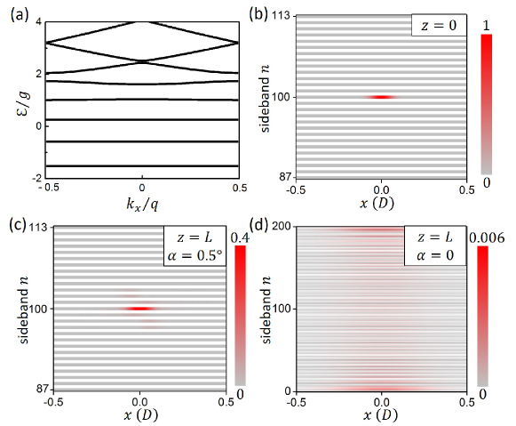
Figure 4: (a) The projected bandstructure showing the formation of Landau levels. $\kappa=0.1g(\pi/2q)^{2}$. (b) The normalized intensity as a function of position and sidebands for the input probe field. The input field has a frequency of $100.8\omega_{m}$. (c) and (d) The output field intensity at $z=L$, corresponding to the non-collinear pump geometry in Fig. 1(c) and the collinear pump geometry in Fig. 1(b).

For electrons in two dimensions, an important consequence of a perpendicular magnetic field is the existence of Landau level — a bulk band with its energy completely independent of the in-plane wavevectors. For photons, Landau level has been observed in rechstman12 , which relies upon a sophisticated dielectric geometry. In contrast, here we show that one can directly generate the Landau level for photons by choosing the right parameters in systems undergoing molecular modulation (Fig. 4). As an illustration, here we choose a larger $g=10^{3}$ m^-1, and keep all other system parameters as in Fig. 3, except without the additional of the two-level atoms. In general, the underlying bandstructure of the system, in the absence of the effective magnetic field, is a tight-binding band along the frequency axis. The use of a larger $g$ ensures that such tight-binding band can be approximated by a parabolic band over a large range of $\mathcal{E}$, which facilitates the creation of the Landau level in the presence of the effective magnetic field. Fig. 4(a) shows the projected bulk band structure calculation for the system shown in Fig. 1(c), where the non-collinear pump creates an effective magnetic field. We indeed observe that the lowest five bands are almost completely flat in the $k_{x}$ and $k_{\omega}$ plane, signifying the creation of the Landau level. As a demonstration of the effect of the Landau level, we input the same probe beam as in Fig. 3, but with a frequency centered at $100.8\omega_{m}$, as shown in Fig. 4(b). We see that the probe field does not diffract in the spatial dimension and also shows no frequency conversion (Fig. 4(c)). This is a direct evidence of Landau levels – the flattened bands prevent diffraction as well as frequency conversion. Our system here therefore provides a novel mechanism to guide light with light. Unlike conventional waveguides, in which light is guided in a well-defined core region, here guiding occurs for every spatial and spectral position inside the “bulk”. We compare our results with the evolution of the probe with a collinear pump geometry, i.e. $\alpha=0$ (Fig. 1(b)). In this case, we choose the same input probe beam as shown in Fig. 4(b). Again, significant diffraction and frequency conversion occurs, as seen in Fig. 4(d).

From a theoretical point of view, to observe the effect of the gauge potential, it is important to keep the diffraction term (i.e. the term containing $\partial^{2}/\partial x^{2}$) in Eq. (1) when describing the probe. Our theoretical treatment therefore is in contrast with the standard treatment of molecular modulation process where the diffraction term is typically ignored.

In the simulations above, we treat the probe field in Eq. (14) as a monochromatic field. Our results are also valid if the pumps and the probe are pulses, as long as the temporal duration of the pulses are long such that the slowly-varying-envelope approximation is valid. Using a long pump pulse, the coherence can be prepared via the “adiabatic following” scheme eberlybook , in which a large coherence can be achieved by setting a negative $\Delta\omega$ and by adiabatically increasing the strength of the pump fields until $|\rho_{ab}|=1/2$ is reached. We give an example of the typical time scale of pulses in a possible experiment. For the pump one can use a $\sim 500$ fs pulse, which has a the spectral width of $\delta\omega_{\mathrm{FWHM}}/\omega_{\mathrm{pump}}\sim 10^{-3}$. For such a pump one can assume that $q$ is a constant in Eq. (13). A typical molecular modulation process requires a dephasing time of the coherence long enough so it works in the transient regime before the coherence has time to decay sokolovbook . Therefore, to study the interaction of a probe pulse with the coherence, one can send in the probe pulse at a time delay. For example, one can use a $\sim 500$ fs probe pulse at a time delay $\sim 1$ ps with respect to the pump. Alternatively, one can also use the long pump pulses $\sim 1$ ns and send the probe into the medium while the pumps are on. In this case, one can choose the frequencies of the pump and the probe to be sufficiently different and observe the predicted topological effects in the sidebands associated with the probe.

In our simulation, we consider the diffraction effects along only one spatial dimension (the $x$-dimension). One can choose the spatial profile of the beam such that the diffraction effect along the $y$-direction to be sufficiently weak. On the other hand, by including diffraction effects along both the $x$ and $y$-dimensions, one may also explore three-dimensional gauge field physics lu16 ; slobozhanyuk16 .

In summary, we study the process of the coherent Raman sideband generation by the molecular modulation with a non-collinear pump geometry. We show that such a geometry provides a synthetic gauge potential for a probe beam sent into the same system. The gauge potential can introduce non-trivial topological effects for the probe beam. Our work identifies a previously unexplored route towards creating topological photonics effects, and highlights an important connection between topological photonics and nonlinear optics.

- (1) R. W. Boyd, Nonlinear Optics 3rd. ed. (Academic Press, Burlington, MA 2008).
- (2) S. E. Harris and A. V. Sokolov, Phys. Rev. Lett. 81, 2894 (1998).
- (3) A. V. Sokolov, D. R. Walker, D. D. Yavuz, G. Y. Yin, and S. E. Harris, Phys. Rev. Lett. 85, 562 (2000).
- (4) A. V. Sokolov and S. E. Harris, J. Opt. B: Quantum Semiclass. Opt. 5, R1 (2003).
- (5) D. D. Yavuz, D. R. Walker, and M. Y. Shverdin, Phys. Rev. A 67, 041803(R) (2003).
- (6) S. W. Huang, W. -J. Chen, and A. H. Kung, Phys. Rev. A 74, 063825 (2006).
- (7) D. D. Yavuz, Phys. Rev. A 75, 041802(R) (2007).
- (8) T. Suzuki, M. Hirai, and M. Katsuragawa, Phys. Rev. Lett. 101, 243602 (2008).
- (9) Y. Y. Wang, C. Wu, F. Couny, M. G. Raymer, and F. Benabid, Phys. Rev. Lett. 105, 123603 (2010).
- (10) S. Baker, I. A. Walmsley, J. W. G. Tisch, and J. P. Marangos, Nat. Photonics 5, 664 (2011).
- (11) M. Zhi and A. V. Sokolov, Opt. Lett. 32, 2251 (2007).
- (12) K. Wang, M. Zhi, X. Hua, J. Strohaber, and A. V. Sokolov, Appl. Opt. 53, 2866 (2014).
- (13) J. Strohaber, M. Zhi, A. V. Sokolov, A. A. Kolomenskii, G. G. Paulus, and H. A. Schuessler, Opt. Lett. 37, 3411 (2012).
- (14) J. Strohaber, J. Abul, M. Richardson, F. Zhu, A. A. Kolomenskii, and H. A. Schuessler, Opt. Express 23, 22463 (2015).
- (15) M. Hafezi, E. A. Demler, M. D. Lukin, and J. M. Taylor, Nature Phys. 7, 907 (2011).
- (16) R. O. Umucalilar and I. Carusotto, Phys. Rev. A 84, 043804 (2011).
- (17) K. Fang, Z. Yu, and S. Fan, Phys. Rev. Lett. 108, 153901 (2012).
- (18) K. Fang, Z. Yu, and S. Fan, Nat. Photonics 6, 782 (2012).
- (19) M. C. Rechstman, J. M. Zeuner, A. Tünnermann, S. Nolte, M. Segev, and A. Szameit, Nat. Photonics 7, 153 (2012).
- (20) L. D. Tzuang, K. Fang, P. Nussenzveig, S. Fan, and M. Lipson, Nat. Photonics 8, 701 (2014).
- (21) E. Li, B. J. Eggleton, K. Fang, and S. Fan, Nat. Commun. 5, 3225 (2014).
- (22) F. Liu and J. Li, Phys. Rev. Lett. 114, 103902 (2015).
- (23) S. Raghu and F. D. M. Haldane, Phys. Rev. A 78, 033834 (2008).
- (24) F. D. M. Haldane and S. Raghu, Phys. Rev. Lett. 100, 013904 (2008).
- (25) Z. Wang, Y. D. Chong, J. D. Joannopoulos, and M. Soljačić, Phys. Rev. Lett. 100, 013905 (2008).
- (26) A. B. Khanikaev, S. H. Mousavi, W. -K. Tse, M. Kargarian, A. H. MacDonald, and G. Shvets, Nature Mater. 12, 233 (2013).
- (27) M. C. Rechstman, J. M. Zeuner, Y. Plotnik, Y. Lumer, D. Podolsky, F. Dreisow, S. Nolte, M. Segev, and A. Szameit, Nature 496, 196 (2013).
- (28) M. Hafezi, S. Mittal, J. Fan, A. Migdall, and J. M. Taylor, Nat. Photonics 7, 1001 (2013).
- (29) S. Mittal, J. Fan, S. Faez, A. Migdall, J. M. Taylor, and M. Hafezi, Phys. Rev. Lett. 113, 087403 (2014).
- (30) L. Lu, J. D. Joannopoulos, and M. Soljačić, Nat. Photonics 8, 821 (2014).
- (31) A. Celi, P. Massignan, J. Ruseckas, N. Goldman, I. B. Spielman, G. Juzeliūnas, and M. Lewenstein, Phys. Rev. Lett. 112, 043001 (2014).
- (32) X.-W. Luo, X. Zhou, C.-F. Li, J.-S. Xu, G.-C. Guo, and Z.-W. Zhou, Nat. Commun. 6, 7704 (2014).
- (33) D.-w. Wang, H. Cai, L. Yuan, S.-y Zhu, and R.-b Liu, Optica 2, 712 (2015).
- (34) F. Le Kien, K. Hakuta, and A. V. Sokolov, Phys. Rev. A 66, 023813 (2002).
- (35) From Eq. (13), Eq. (14) is valid when . This condition is satisfied in this letter.
- (36) L. Yuan, Y. Shi, and S. Fan, Opt. Lett. 41, 741 (2016).
- (37) T. Ozawa, H. M. Price, N. Goldman, O. Zilberberg, and I. Carusotto, Phys. Rev. A 93, 043827 (2016).
- (38) D. J. Thouless, M. Kohmoto, M. P. Nightingale, and M. den Nijs, Phys. Rev. Lett. 49, 405 (1982).
- (39) L. Allen and J. H. Eberly, Optical Resonance and Two-level Atoms (Dover, New York, 1987).
- (40) T. J. Hall and S. V. Gaponenko eds., Extreme Photonics & Applications (Springer Netherlands, 2010).
- (41) L. Lu, C. Fang, L. Fu, S. G. Johnson, J. D. Joannopoulos, and M. Soljačić, Nat. Phys. 12, 337 (2016).
- (42) A. Slobozhanyuk, S. H. Mousavi, X. Ni, D. Smirnova, Y. S. Kivshar, and A. B. Khanikaev, arXiv:1602.00049 (2016).