IFT-UAM/CSIC-16-140

FTUAM-16-48

January 2018

On the perturbative renormalisation of

four-quark operators for new physics

M. Papinutto,^a C. Pena,^b,c D. Preti^c

^a Dipartimento di Fisica, “Sapienza” Università di Roma, and INFN, Sezione di Roma

Piazzale A. Moro 2, I-00185 Roma, Italy

^b Departamento de Física Teórica, Universidad Autónoma de Madrid

Cantoblanco E-28049 Madrid, Spain

^c Instituto de Física Teórica UAM-CSIC

c/Nicolás Cabrera 13-15, Universidad Autónoma de Madrid

Cantoblanco E-28049 Madrid, Spain

Abstract: We discuss the renormalisation properties of the full set of $\Delta F=2$ operators involved in BSM processes, including the definition of RGI versions of operators that exhibit mixing under RG transformations. As a first step for a fully non-perturbative determination of the scale-dependent renormalization factors and their runnings, we introduce a family of appropriate Schrödinger Functional schemes, and study them in perturbation theory. This allows, in particular, to determine the NLO anomalous dimensions of all $\Delta F=1,2$ operators in these schemes. Finally, we discuss the systematic uncertainties related to the use of NLO perturbation theory for the RG running of four-quark operators to scales in the GeV range, in both our SF schemes and standard ${\overline{\rm MS}}$ and RI-MOM schemes. Large truncation effects are found for some of the operators considered.

1 Introduction

Hadronic matrix elements of four-quark operators play an important rôle in the study of flavour physics within the Standard Model (SM), as well as in searches for new physics. In particular, they are essential to the study of CP-violation in the hadron sector in both the SM and beyond-the-SM (BSM) models, where they parametrise the effect of new interactions. A key ingredient of these studies is the renormalisation of the operators, including their renormalisation group (RG) running from low-energy hadronic scales $\mathcal{O}(\Lambda_{\rm\scriptscriptstyle QCD})$ to the high-energy electroweak or new physics scales, where contact with the fundamental underlying theory is made.

In this paper we prepare the ground for a full non-perturbative computation of the low-energy renormalisation and RG running of all possible four-quark operators with net flavour change, by introducing appropriate Schrödinger Functional (SF) renormalisation schemes. In order to connect them with standard ${\overline{\rm MS}}$ schemes at high energies, as well as with renormalisation group invariant (RGI) operators, it is however still necessary to compute the relevant scheme matching factors perturbatively. We compute the latter at one loop, which, in particular, allows us to determine the complete set of next-to-leading (NLO) anomalous dimensions in our SF schemes.

An interesting byproduct of our computation is the possibility to study the systematic uncertainties related to the use of NLO perturbation theory in the computation of the RG running of four-quark operators to hadronic scales. This is a common feature of the phenomenological literature, and the question can be posed whether perturbative truncation effects can have an impact in physics analyses. The latter are studied in detail in our SF schemes, as well as in the ${\overline{\rm MS}}$ and RI-MOM schemes that have been studied in the literature. One of our main conclusions is that perturbative truncation effects in RG running can be argued to be significantly large. This makes a very strong case for a fully non-perturbative RG running programme for these operators.

The structure of the paper is as follows. In Section 2 we provide a short review of the renormalisation properties of the full basis of $\Delta F=2$ four-quark operators, stressing how considering it also allows to obtain the anomalous dimensions of $\Delta F=1$ operators. We focus on the operators that appear in BSM physics, which exhibit scale-dependent mixing under renormalisation, and discuss the definition of RGI operators in that case. In Section 3 we introduce our SF schemes, and explain the strategy to obtain NLO anomalous dimensions in the latter through a one-loop computation of the relevant four- and two-point correlation functions. Finally, in Section 4 we carry out a systematic study of the perturbative RG running in several schemes, and provide estimates of the resulting truncation uncertainty at scales in the few GeV range. In order to improve readability, several tables and figures are collected after the main text, and a many technical details are discussed in appendices.

2 Renormalisation of four-quark operators

2.1 Mixing of four-quark operators under renormalisation

The mixing under renormalisation of four-quark operators that do not require subtraction of lower-dimensional operators has been determined in full generality in [1]. The absence of subtractions is elegantly implemented by using a formalism in which the operators are made of four different quark flavours; a complete set of Lorentz-invariant operators is

$$\begin{array}[]{l@{}l@{}l@{\hspace{20mm}}l@{}l@{}l}Q_{1}^{\pm}&\,\,=&{\cal O}^{\pm}_{\rm VV+AA}\,,\hfil\hskip 56.9055pt&{\cal Q}_{1}^{\pm}&\,\,=&{\cal O}^{\pm}_{\rm VA+AV}\,,\\[4.30554pt] Q_{2}^{\pm}&\,\,=&{\cal O}^{\pm}_{\rm VV-AA}\,,\hfil\hskip 56.9055pt&{\cal Q}_{2}^{\pm}&\,\,=&{\cal O}^{\pm}_{\rm VA-AV}\,,\\[4.30554pt] Q_{3}^{\pm}&\,\,=&{\cal O}^{\pm}_{\rm SS-PP}\,,\hfil\hskip 56.9055pt&{\cal Q}_{3}^{\pm}&\,\,=&{\cal O}^{\pm}_{\rm PS-SP}\,,\\[4.30554pt] Q_{4}^{\pm}&\,\,=&{\cal O}^{\pm}_{\rm SS+PP}\,,\hfil\hskip 56.9055pt&{\cal Q}_{4}^{\pm}&\,\,=&{\cal O}^{\pm}_{\rm PS+SP}\,,\\[4.30554pt] Q_{5}^{\pm}&\,\,=&-2{\cal O}^{\pm}_{\rm TT}\,,\hfil\hskip 56.9055pt&{\cal Q}_{5}^{\pm}&\,\,=&-2{\cal O}^{\pm}_{\rm T\tilde{T}}\,,\end{array}$$ (2.6)

where

$${\cal O}^{\pm}_{\Gamma_{1}\Gamma_{2}}=\frac{1}{2}\left[(\bar{\psi}_{1}\Gamma_{1}\psi_{2})(\bar{\psi}_{3}\Gamma_{2}\psi_{4})\,\pm\,(\bar{\psi}_{1}\Gamma_{1}\psi_{4})(\bar{\psi}_{3}\Gamma_{2}\psi_{2})\right]\,,$$ (2.7)

${\cal O}^{\pm}_{\Gamma_{1}\Gamma_{2}\pm\Gamma_{2}\Gamma_{1}}\equiv{\cal O}^{\pm}_{\Gamma_{1}\Gamma_{2}}\pm{\cal O}^{\pm}_{\Gamma_{2}\Gamma_{1}}$, and the labeling is adopted ${\rm V}\to\gamma_{\mu}$, ${\rm A}\to\gamma_{\mu}\gamma_{5}$, ${\rm S}\to\mathbf{1}$, ${\rm P}\to\gamma_{5}$, ${\rm T}\to\sigma_{\mu\nu}$, ${\rm\tilde{T}}\to{\scriptstyle{{1\over 2}}}\varepsilon_{\mu\nu\rho\tau}\sigma_{\rho\tau}$, with $\sigma_{\mu\nu}={\scriptstyle{{i\over 2}}}[\gamma_{\mu},\gamma_{\nu}]$. In the above expression round parentheses indicate spin and colour scalars, and subscripts are flavour labels. Note that operators $Q_{k}^{\pm}$ are parity-even, and ${\cal Q}_{k}^{\pm}$ are parity-odd.

It is important to stress that this framework is fairly general. For instance, with the assignments

$$\psi_{1}=\psi_{3}=s\,,~{}~{}~{}~{}~{}\psi_{2}=\psi_{4}=d$$ (2.8)

the operators $Q_{k}^{-}$ vanish, while $Q_{1}^{+}$ enters the SM amplitude for $K^{0}$–$\bar{K}^{0}$ mixing, and $Q_{2,\ldots,5}^{+}$ the contributions to the same amplitude from arbitrary extensions of the SM. Idem for $B_{(s)}^{0}$–$\bar{B}_{(s)}^{0}$ mixing with

$$\psi_{1}=\psi_{3}=b\,,~{}~{}~{}~{}~{}\psi_{2}=\psi_{4}=d/s\,.$$ (2.9)

If one instead chooses the assignments

$$\begin{split}&\psi_{1}=s\,,~{}~{}~{}\psi_{2}=d\,,~{}~{}~{}\psi_{3}=\psi_{4}=u,c\,,\\ &\psi_{1}=s\,,~{}~{}~{}\psi_{4}=d\,,~{}~{}~{}\psi_{2}=\psi_{3}=u,c\,,\end{split}$$ (2.10)

the resulting $Q_{1}^{\pm}$ will be the operators in the SM $\Delta S=1$ effective weak Hamiltonian with an active charm quark, which, in the chiral limit, do not mix with lower-dimensional operators. By proceeding in this way, essentially all possible four-quark effective interactions with net flavour change can be easily seen to be comprised within our scope.

In the following we will assume a mass-independent renormalisation scheme. Renormalised operators can be written as

$$\begin{split}\bar{Q}_{k}^{\pm}&=Z_{kl}^{\pm}(\delta_{lm}+\Delta_{lm}^{\pm})Q_{m}^{\pm}\,,\\ \bar{\cal Q}_{k}^{\pm}&={\cal Z}_{kl}^{\pm}(\delta_{lm}+\mbox{\textcyr{D}}_{lm}^{\pm}){\cal Q}_{m}^{\pm}\end{split}$$ (2.11)

(summations over $l,m$ are implied), where the matrices $Z,{\cal Z}$ are scale-dependent and reabsorb logarithmic divergences, while $\Delta,\mbox{\textcyr{D}}$ are (possible) finite subtraction coefficients that only depend on the bare coupling. They have the generic structure

$$Z=\left(\begin{array}[]{ccccc}Z_{11}&0&0&0&0\\ 0&Z_{22}&Z_{23}&0&0\\ 0&Z_{32}&Z_{33}&0&0\\ 0&0&0&Z_{44}&Z_{45}\\ 0&0&0&Z_{54}&Z_{55}\end{array}\right)\,,\qquad\Delta=\left(\begin{array}[]{ccccc}0&\Delta_{12}&\Delta_{13}&\Delta_{14}&\Delta_{15}\\ \Delta_{21}&0&0&\Delta_{24}&\Delta_{25}\\ \Delta_{31}&0&0&\Delta_{34}&\Delta_{35}\\ \Delta_{41}&\Delta_{42}&\Delta_{43}&0&0\\ \Delta_{51}&\Delta_{52}&\Delta_{53}&0&0\end{array}\right)\,,$$ (2.22)

and similarly in the parity-odd sector. If chiral symmetry is preserved by the regularization, both $\Delta$ and D vanish. The main result of [1] is that $\mbox{\textcyr{D}}=0$ even when a lattice regularisation that breaks chiral symmetry explicitly through the Wilson term is employed, due to the presence of residual discrete flavour symmetries. In particular, the left-left operators ${\cal O}_{\rm VA+AV}^{\pm}$ that mediate Standard Model-allowed transitions renormalise multiplicatively, while operators that appear as effective interactions in extensions of the Standard Model do always mix.

Interestingly, in [1] some identities are derived that relate the renormalisation matrices for $({\cal Q}_{2}^{+},{\cal Q}_{3}^{+})$ and $({\cal Q}_{2}^{-},{\cal Q}_{3}^{-})$ in RI-MOM schemes. In Appendix A we discuss the underlying symmetry structure in some more detail, and show how it can be used to derive constraints between matrices of anomalous dimensions in generic schemes.

2.2 Callan-Symanzik equations

Theory parameters and operators are renormalised at the renormalisation scale $\mu$. The scale dependence of renormalised quantities is then governed by renormalisation group evolution. We will consider QCD with $N_{\mathrm{\scriptstyle f}}$ quark flavours and $N$ colours. The Callan-Symanzik equations satisfied by the gauge coupling and quark masses are of the form

$$q\frac{\rm d}{{\rm d}q}\kern 1.0pt\overline{\kern-1.0ptg\kern 0.0pt}\kern 1.0pt(q) =\beta(\kern 1.0pt\overline{\kern-1.0ptg\kern 0.0pt}\kern 1.0pt(q))\,,$$ (2.23)

$$q\frac{\rm d}{{\rm d}q}\kern 2.0pt\overline{\kern-1.0ptm\kern-1.0pt}\kern 1.0pt_{\rm f}(q) =\tau(\kern 1.0pt\overline{\kern-1.0ptg\kern 0.0pt}\kern 1.0pt(q))\kern 2.0pt\overline{\kern-1.0ptm\kern-1.0pt}\kern 1.0pt_{\rm f}(q)\,,$$ (2.24)

respectively, and satisfy the initial conditions

$$\kern 1.0pt\overline{\kern-1.0ptg\kern 0.0pt}\kern 1.0pt(\mu) =g_{\rm R}\,,$$ (2.25)

$$\kern 2.0pt\overline{\kern-1.0ptm\kern-1.0pt}\kern 1.0pt_{\rm f}(\mu) =m_{{\rm R},\rm f}\,,$$ (2.26)

where ${\rm f}$ is a flavour label. Mass-independence of the scheme is reflected in the fact that the beta function and mass anomalous dimension $\tau$ depend on the coupling and the number of flavours, but not on quark masses. Asymptotic perturbative expansions read

$$\beta(g) \underset{g\sim 0}{\approx}-g^{3}(b_{0}+b_{1}g^{2}+\ldots)\,,$$ (2.27)

$$\tau(g) \underset{g\sim 0}{\approx}-g^{2}(d_{0}+d_{1}g^{2}+\ldots)\,.$$ (2.28)

The universal coefficients of the perturbative beta function and mass anomalous dimension are

$$\begin{split}b_{0}&=\frac{1}{(4\pi)^{2}}\left[\frac{11}{3}N-\frac{2}{3}N_{\mathrm{\scriptstyle f}}\right]\,,\\ b_{1}&=\frac{1}{(4\pi)^{4}}\left[\frac{34}{3}N^{2}-\left(\frac{13}{3}N-\frac{1}{N}\right)N_{\mathrm{\scriptstyle f}}\right]\,,\\ d_{0}&=\frac{1}{(4\pi)^{2}}\,\frac{3(N^{2}-1)}{N}\,.\end{split}$$ (2.29)

We will deal with Euclidean correlation functions of gauge-invariant composite operators. Without loss of generality, let us consider correlation functions of the form

$$G_{k}(x;y_{1},\ldots,y_{n})=\langle O_{k}(x){\cal O}_{1}(y_{1})\cdots{\cal O}_{n}(y_{n}))\rangle\,,$$ (2.30)

with $x\neq y_{j}~{}\forall j,~{}y_{j}\neq y_{k}~{}\forall j\neq k$, where $\{O_{k}\}$ is a set of operators that mix under renormalisation, and where ${\cal O}_{k}$ are multiplicatively renormalisable operators. Renormalised correlation functions satisfy a system of Callan-Symanzik equations obtained by imposing that $G_{k}$ is independent of the renormalisation scale $\mu$, viz.

$$\mu\frac{{\rm d}}{{\rm d}\mu}\bar{G}_{j}=\sum_{k}\left[\gamma_{jk}(g_{\rm R})+\sum_{l=1}^{n}\tilde{\gamma}_{l}(g_{\rm R})\delta_{jk}\right]\bar{G}_{k}\,,$$ (2.31)

which, expanding the total derivative, leads to

$$\left\{\mu\frac{\partial}{\partial\mu}+\beta(g_{\rm R})\frac{\partial}{\partial g_{\rm R}}+\beta_{\lambda}(g_{\rm R})\lambda\,\frac{\partial}{\partial\lambda}+\sum_{{\rm f}=1}^{N_{\mathrm{\scriptstyle f}}}\tau(g_{\rm R})m_{{\rm R},\rm f}\frac{\partial}{\partial m_{{\rm R},\rm f}}-\sum_{l=1}^{n}\tilde{\gamma}_{l}(g_{\rm R})\right\}\bar{G}_{j}=\sum_{k}\gamma_{jk}(g_{\rm R})\,\bar{G}_{k}\,,$$ (2.32)

where $\gamma$ is a matrix of anomalous dimensions describing the mixing of $\{O_{k}\}$, and $\tilde{\gamma}_{l}$ is the anomalous dimension of ${\cal O}_{l}$. For completeness, we have included a term which takes into account the dependence on the gauge parameter $\lambda$ in covariant gauges; this term is absent in schemes like ${\overline{\rm MS}}$ (irrespective of the regularisation prescription) or the SF schemes we will introduce, but is present in the RI schemes we will also be concerned with later. The RG function $\beta_{\lambda}$ is given by

$$q\frac{\rm{d}}{{\rm d}q}\lambda(q)=\beta_{\lambda}(\kern 1.0pt\overline{\kern-1.0ptg\kern 0.0pt}\kern 1.0pt(q))\lambda(q)\,,$$ (2.33)

and its perturbative expansion has the form

$$\beta_{\lambda}(g)=-g^{2}(b_{0}^{\lambda}+b_{1}^{\lambda}g^{2}+\ldots)\,,$$ (2.34)

where the universal coefficient is given by

$$b_{0}^{\lambda}=\frac{1}{(4\pi)^{2}}\left[\left(\lambda-\frac{13}{3}\right)N+\frac{4}{3}N_{\mathrm{\scriptstyle f}}\right]\,.$$ (2.35)

In the Landau gauge ($\lambda=0$) the term with $\beta_{\lambda}$ always vanishes. From now on, in order to avoid unnecessary complications, we will assume that whenever RI anomalous dimensions are employed they will be in Landau gauge, and consequently drop terms with $\beta_{\lambda}$ in all equations.

From now on, in order to simplify the notation we will use the shorthand notation

$$q\frac{\rm{d}}{{\rm d}q}\kern 3.0pt\overline{\kern-2.0ptO\kern 0.0pt}\kern 1.0pt_{j}(q)=\sum_{k}\gamma_{jk}(\kern 1.0pt\overline{\kern-1.0ptg\kern 0.0pt}\kern 1.0pt(q))\kern 3.0pt\overline{\kern-2.0ptO\kern 0.0pt}\kern 1.0pt_{k}(q)$$ (2.36)

for the Callan-Symanzik equation satisfied by the insertion of a composite operator in a renormalised, on-shell correlation function (i.e. Eq. (2.36) is to be interpreted in the sense provided by Eq. (2.32)). The corresponding initial condition can be written as

$$\kern 3.0pt\overline{\kern-2.0ptO\kern 0.0pt}\kern 1.0pt_{k}(\mu)={O_{\rm R}}_{,k}\,,$$ (2.37)

and the perturbative expansion of the anomalous dimension matrix $\gamma$ as

$$\gamma(g)\underset{g\sim 0}{\approx}-g^{2}(\gamma_{0}+\gamma_{1}g^{2}+\ldots)\,.$$ (2.38)

The universal, one-loop coefficients of the anomalous dimension matrix for four-fermion operators were first computed in [5, 6] and [7]. With our notational conventions the non-zero entries read

$$\begin{split}\gamma^{+,(0)}_{11}&=\left(6-\frac{6}{N}\right)(4\pi)^{-2}\,,\\ \gamma^{+,(0)}_{22}&=\left(\frac{6}{N}\right)(4\pi)^{-2}\,,\\ \gamma^{+,(0)}_{23}&=12(4\pi)^{-2}\,,\\ \gamma^{+,(0)}_{33}&=\left(-6N+\frac{6}{N}\right)(4\pi)^{-2}\,,\\ \gamma^{+,(0)}_{44}&=\left(6-6N+\frac{6}{N}\right)(4\pi)^{-2}\,,\\ \gamma^{+,(0)}_{45}&=\left(\frac{1}{2}-\frac{1}{N}\right)(4\pi)^{-2}\,,\\ \gamma^{+,(0)}_{54}&=\left(-24-\frac{48}{N}\right)(4\pi)^{-2}\,,\\ \gamma^{+,(0)}_{55}&=\left(6+2N-\frac{2}{N}\right)(4\pi)^{-2}\,,\end{split}\quad\quad\quad\quad\begin{split}\gamma^{-,(0)}_{11}&=\left(-6-\frac{6}{N}\right)(4\pi)^{-2}\,,\\ \gamma^{-,(0)}_{22}&=\left(\frac{6}{N}\right)(4\pi)^{-2}\,,\\ \gamma^{-,(0)}_{23}&=-12(4\pi)^{-2}\,,\\ \gamma^{-,(0)}_{33}&=\left(-6N+\frac{6}{N}\right)(4\pi)^{-2}\,,\\ \gamma^{-,(0)}_{44}&=\left(-6-6N+\frac{6}{N}\right)(4\pi)^{-2}\,,\\ \gamma^{-,(0)}_{45}&=\left(-\frac{1}{2}-\frac{1}{N}\right)(4\pi)^{-2}\,,\\ \gamma^{-,(0)}_{54}&=\left(24-\frac{48}{N}\right)(4\pi)^{-2}\,,\\ \gamma^{-,(0)}_{55}&=\left(-6+2N-\frac{2}{N}\right)(4\pi)^{-2}\,.\end{split}$$ (2.39)

2.3 Formal solution of the RG equation

Let us now consider the solution to Eq. (2.36). To that purpose we start by introducing the (matricial) renormalisation group evolution operator $U(\mu_{2},\mu_{1})$ that evolves renormalised operators between the scales $\mu_{1}$ and $\mu_{2}<\mu_{1}$,

$$\kern 3.0pt\overline{\kern-2.0ptO\kern 0.0pt}\kern 1.0pt_{i}(\mu_{2})=U_{ij}(\mu_{2},\mu_{1})\kern 3.0pt\overline{\kern-2.0ptO\kern 0.0pt}\kern 1.0pt_{j}(\mu_{1})\,.$$ (2.40)

By substituting into Eq. (2.36) one has the equation for $U(\mu_{2},\mu_{1})$

$$\mu_{2}\,\frac{\rm{d}}{{\rm d}\mu_{2}}\,U(\mu_{2},\mu_{1})=\gamma[\kern 1.0pt\overline{\kern-1.0ptg\kern 0.0pt}\kern 1.0pt(\mu_{2})]U(\mu_{2},\mu_{1})\,,$$ (2.41)

(n.b. the matrix product on the r.h.s.) with initial condition $U(\mu_{1},\mu_{1})=\mathbf{1}$. Following a standard procedure, this differential equation for $U$ can be converted into a Volterra-type integral equation and solved iteratively, viz.

$$U(\mu_{2},\mu_{1})={\rm T}\kern-2.0pt\exp\left\{\int_{\kern 1.0pt\overline{\kern-1.0ptg\kern 0.0pt}\kern 1.0pt(\mu_{1})}^{\kern 1.0pt\overline{\kern-1.0ptg\kern 0.0pt}\kern 1.0pt(\mu_{2})}\kern-8.0pt{\rm d}g\,\frac{1}{\beta(g)}\,\gamma(g)\right\}\,,$$ (2.42)

where as usual the notation ${\rm T}\kern-2.0pt\exp$ refers to a definition in terms of the Taylor expansion of the exponential function with “powers” of the integral involving argument-ordered integrands — explicitly, for a generic matrix function $M$, one has

$$\begin{split}{\rm T}\kern-2.0pt\exp\left\{\int_{x_{-}}^{x_{+}}\kern-8.0pt{\rm d}x\,M(x)\right\}\equiv\mathbf{1}&+\int_{x_{-}}^{x_{+}}\kern-8.0pt{\rm d}x\,M(x)\\ &+\int_{x_{-}}^{x_{+}}\kern-8.0pt{\rm d}x_{1}\,M(x_{1})\int_{x_{-}}^{x_{1}}\kern-8.0pt{\rm d}x_{2}\,M(x_{2})\\ &+\int_{x_{-}}^{x_{+}}\kern-8.0pt{\rm d}x_{1}\,M(x_{1})\int_{x_{-}}^{x_{1}}\kern-8.0pt{\rm d}x_{2}\,M(x_{2})\int_{x_{-}}^{x_{2}}\kern-8.0pt{\rm d}x_{3}\,M(x_{3})\\ &+\ldots\\ =\mathbf{1}&+\int_{x_{-}}^{x_{+}}\kern-8.0pt{\rm d}x\,M(x)\\ &+\frac{1}{2!}\int_{x_{-}}^{x_{+}}\kern-8.0pt{\rm d}x_{1}\int_{x_{-}}^{x_{+}}\kern-8.0pt{\rm d}x_{2}\,\Big{\{}\theta(x_{1}-x_{2})M(x_{1})M(x_{2})+\\ &~{}~{}~{}~{}~{}~{}~{}~{}~{}~{}~{}~{}~{}~{}~{}~{}~{}~{}~{}~{}~{}~{}~{}~{}~{}~{}~{}~{}~{}\theta(x_{2}-x_{1})M(x_{2})M(x_{1})\Big{\}}\\ &+\ldots\end{split}$$ (2.43)

2.4 RGI in the absence of mixing

Let us now consider an operator $O$ that renormalises multiplicatively. In that case, both $\gamma$ and $U$ are scalar objects, and Eq. (2.40) can be manipulated as

$$\begin{split}\kern 3.0pt\overline{\kern-2.0ptO\kern 0.0pt}\kern 1.0pt(\mu_{2})&=\exp\left\{\int_{\kern 1.0pt\overline{\kern-1.0ptg\kern 0.0pt}\kern 1.0pt(\mu_{1})}^{\kern 1.0pt\overline{\kern-1.0ptg\kern 0.0pt}\kern 1.0pt(\mu_{2})}\kern-8.0pt{\rm d}g\,\frac{\gamma(g)}{\beta(g)}\right\}\kern 3.0pt\overline{\kern-2.0ptO\kern 0.0pt}\kern 1.0pt(\mu_{1})\\ &=\exp\left\{\int_{\kern 1.0pt\overline{\kern-1.0ptg\kern 0.0pt}\kern 1.0pt(\mu_{1})}^{\kern 1.0pt\overline{\kern-1.0ptg\kern 0.0pt}\kern 1.0pt(\mu_{2})}\kern-8.0pt{\rm d}g\,\frac{\gamma_{0}}{b_{0}g}\right\}\exp\left\{\int_{\kern 1.0pt\overline{\kern-1.0ptg\kern 0.0pt}\kern 1.0pt(\mu_{1})}^{\kern 1.0pt\overline{\kern-1.0ptg\kern 0.0pt}\kern 1.0pt(\mu_{2})}\kern-8.0pt{\rm d}g\,\left[\frac{\gamma(g)}{\beta(g)}-\frac{\gamma_{0}}{b_{0}g}\right]\right\}\kern 3.0pt\overline{\kern-2.0ptO\kern 0.0pt}\kern 1.0pt(\mu_{1})\\ &=\left[\frac{\kern 1.0pt\overline{\kern-1.0ptg\kern 0.0pt}\kern 1.0pt^{2}(\mu_{2})}{\kern 1.0pt\overline{\kern-1.0ptg\kern 0.0pt}\kern 1.0pt^{2}(\mu_{1})}\right]^{\frac{\gamma_{0}}{2b_{0}}}\exp\left\{\int_{\kern 1.0pt\overline{\kern-1.0ptg\kern 0.0pt}\kern 1.0pt(\mu_{1})}^{\kern 1.0pt\overline{\kern-1.0ptg\kern 0.0pt}\kern 1.0pt(\mu_{2})}\kern-8.0pt{\rm d}g\,\left[\frac{\gamma(g)}{\beta(g)}-\frac{\gamma_{0}}{b_{0}g}\right]\right\}\kern 3.0pt\overline{\kern-2.0ptO\kern 0.0pt}\kern 1.0pt(\mu_{1})\,,\end{split}$$ (2.44)

yielding the identity

$$\left[\frac{\kern 1.0pt\overline{\kern-1.0ptg\kern 0.0pt}\kern 1.0pt^{2}(\mu_{2})}{4\pi}\right]^{-\frac{\gamma_{0}}{2b_{0}}}\kern 3.0pt\overline{\kern-2.0ptO\kern 0.0pt}\kern 1.0pt(\mu_{2})=\left[\frac{\kern 1.0pt\overline{\kern-1.0ptg\kern 0.0pt}\kern 1.0pt^{2}(\mu_{1})}{4\pi}\right]^{-\frac{\gamma_{0}}{2b_{0}}}\exp\left\{\int_{\kern 1.0pt\overline{\kern-1.0ptg\kern 0.0pt}\kern 1.0pt(\mu_{1})}^{\kern 1.0pt\overline{\kern-1.0ptg\kern 0.0pt}\kern 1.0pt(\mu_{2})}\kern-8.0pt{\rm d}g\,\left[\frac{\gamma(g)}{\beta(g)}-\frac{\gamma_{0}}{b_{0}g}\right]\right\}\kern 3.0pt\overline{\kern-2.0ptO\kern 0.0pt}\kern 1.0pt(\mu_{1})\,.$$ (2.45)

The advantage of having rewritten Eq. (2.40) in this way is that now the integral in the exponential is finite as either integration limit is taken to zero; in particular, the r.h.s. is well-defined when $\mu_{2}\to\infty~{}\Leftrightarrow~{}\kern 1.0pt\overline{\kern-1.0ptg\kern 0.0pt}\kern 1.0pt(\mu_{2})\to 0$, and therefore so is the l.h.s. Thus, we define the RGI operator insertion as

$$\hat{O}\equiv\lim_{\mu\to\infty}\left[\frac{\kern 1.0pt\overline{\kern-1.0ptg\kern 0.0pt}\kern 1.0pt^{2}(\mu)}{4\pi}\right]^{-\frac{\gamma_{0}}{2b_{0}}}\kern 3.0pt\overline{\kern-2.0ptO\kern 0.0pt}\kern 1.0pt(\mu)\,,$$ (2.46)

upon which we have an explicit expression to retrieve the RGI operator from the renormalised one at any value of the renormalisation scale $\mu$, provided the anomalous dimension and the beta function are known for scales $\geq\mu$,

$$\hat{O}=\left[\frac{\kern 1.0pt\overline{\kern-1.0ptg\kern 0.0pt}\kern 1.0pt^{2}(\mu)}{4\pi}\right]^{-\frac{\gamma_{0}}{2b_{0}}}\exp\left\{-\int_{0}^{\kern 1.0pt\overline{\kern-1.0ptg\kern 0.0pt}\kern 1.0pt(\mu)}\kern-8.0pt{\rm d}g\,\left[\frac{\gamma(g)}{\beta(g)}-\frac{\gamma_{0}}{b_{0}g}\right]\right\}\kern 3.0pt\overline{\kern-2.0ptO\kern 0.0pt}\kern 1.0pt(\mu)\,.$$ (2.47)

Starting from the latter equation, it is easy to check explicitly that $\hat{O}$ is invariant under a change of renormalisation scheme.

Note that the crucial step in the manipulation has been to add and subtract the term $\frac{\gamma_{0}}{b_{0}g}$ in the integral that defines the RG evolution operator, which allows to obtain a quantity that is UV-finite by removing the logarithmic divergence induced at small $g$ by the perturbative behaviour $\gamma(g)/\beta(g)\sim 1/g$. When $\gamma$ is a matrix of anomalous dimensions this step becomes non-trivial, since in general $[\gamma(g),\gamma_{0}]\neq 0$; the derivation has thus to be performed somewhat more carefully.

2.5 RGI in the presence of mixing

Let us start by studying the UV behaviour of the matricial RG evolution operator in Eq. (2.40), using its actual definition in Eq. (2.43). To that purpose, we first observe that by taking the leading-order approximation for $\gamma(g)/\beta(g)$ the T-exponential becomes a standard exponential, since $[\gamma_{0}g_{1}^{2},\gamma_{0}g_{2}^{2}]=0~{}\forall g_{1},g_{2}$. One can then perform the integral trivially and write

$$U(\mu_{2},\mu_{1})\underset{\rm LO}{=}\left[\frac{\kern 1.0pt\overline{\kern-1.0ptg\kern 0.0pt}\kern 1.0pt^{2}(\mu_{2})}{\kern 1.0pt\overline{\kern-1.0ptg\kern 0.0pt}\kern 1.0pt^{2}(\mu_{1})}\right]^{\frac{\gamma_{0}}{2b_{0}}}\equiv U_{\rm\scriptscriptstyle LO}(\mu_{2},\mu_{1})\,.$$ (2.48)

When next-to-leading order corrections are included the T-exponential becomes non-trivial. In order to make contact with the literature (see e.g. [8, 5]), we write

$$U(\mu_{2},\mu_{1})\equiv\left[W(\mu_{2})\right]^{-1}\,U_{\rm\scriptscriptstyle LO}(\mu_{2},\mu_{1})W(\mu_{1})\,.$$ (2.50)

Upon inserting Eq. (2.50) in Eq. (2.41) we obtain for $W$ the RG equation

$$\begin{split}\mu\frac{\rm{d}}{{\rm d}\mu}W(\mu)&=-W(\mu)\gamma(\kern 1.0pt\overline{\kern-1.0ptg\kern 0.0pt}\kern 1.0pt(\mu))+\beta(\kern 1.0pt\overline{\kern-1.0ptg\kern 0.0pt}\kern 1.0pt(\mu))\frac{\gamma_{0}}{b_{0}\kern 1.0pt\overline{\kern-1.0ptg\kern 0.0pt}\kern 1.0pt(\mu)}W(\mu)\\ &=[\gamma(\kern 1.0pt\overline{\kern-1.0ptg\kern 0.0pt}\kern 1.0pt(\mu)),W(\mu)]-\beta(\kern 1.0pt\overline{\kern-1.0ptg\kern 0.0pt}\kern 1.0pt(\mu))\left(\frac{\gamma(\kern 1.0pt\overline{\kern-1.0ptg\kern 0.0pt}\kern 1.0pt(\mu))}{\beta(\kern 1.0pt\overline{\kern-1.0ptg\kern 0.0pt}\kern 1.0pt(\mu))}-\frac{\gamma_{0}}{b_{0}\kern 1.0pt\overline{\kern-1.0ptg\kern 0.0pt}\kern 1.0pt(\mu)}\right)W(\mu)\,.\end{split}$$ (2.51)

The matrix $W$ can be interpreted as the piece of the evolution operator containing contributions beyond the leading perturbative order. It is easy to check by expanding perturbatively (see below) that $W$ is regular in the UV, and that all the logarithmic divergences in the evolution operator are contained in $U_{\rm\scriptscriptstyle LO}$; in particular,

$$W(\mu)\underset{\mu\to\infty}{=}\mathbf{1}\,.$$ (2.52)

Note also that in the absence of mixing Eq. (2.51) can be solved explicitly to get (using $W(\infty)=1$)

$$W(\mu)\underset{\rm no~{}mixing}{=}\exp\left\{-\int_{0}^{\kern 1.0pt\overline{\kern-1.0ptg\kern 0.0pt}\kern 1.0pt(\mu)}\kern-8.0pt{\rm d}g\,\left[\frac{\gamma(g)}{\beta(g)}-\frac{\gamma_{0}}{b_{0}g}\right]\right\}\,.$$ (2.53)

Now it is easy, by analogy with the non-mixing case, to define RGI operators. We rewrite Eq. (2.40) as

$$\left[\frac{\kern 1.0pt\overline{\kern-1.0ptg\kern 0.0pt}\kern 1.0pt^{2}(\mu_{2})}{4\pi}\right]^{-\frac{\gamma_{0}}{2b_{0}}}W(\mu_{2})\kern 3.0pt\overline{\kern-2.0ptO\kern 0.0pt}\kern 1.0pt(\mu_{2})=\left[\frac{\kern 1.0pt\overline{\kern-1.0ptg\kern 0.0pt}\kern 1.0pt^{2}(\mu_{1})}{4\pi}\right]^{-\frac{\gamma_{0}}{2b_{0}}}W(\mu_{1})\kern 3.0pt\overline{\kern-2.0ptO\kern 0.0pt}\kern 1.0pt(\mu_{1})\,,$$ (2.54)

where $\kern 3.0pt\overline{\kern-2.0ptO\kern 0.0pt}\kern 1.0pt$ is a vector of renormalised operators on which the RG evolution matrix acts, cf. Eq. (2.40). The l.h.s. (resp. r.h.s.) is obviously finite for $\mu_{1}\to\infty$ (resp. $\mu_{2}\to\infty$), which implies that the vector of RGI operators can be obtained as

$$\hat{O}=\left[\frac{\kern 1.0pt\overline{\kern-1.0ptg\kern 0.0pt}\kern 1.0pt^{2}(\mu)}{4\pi}\right]^{-\frac{\gamma_{0}}{2b_{0}}}W(\mu)\kern 3.0pt\overline{\kern-2.0ptO\kern 0.0pt}\kern 1.0pt(\mu)\equiv\tilde{U}(\mu)\kern 3.0pt\overline{\kern-2.0ptO\kern 0.0pt}\kern 1.0pt(\mu)\,.$$ (2.55)

When there is no mixing, the use of Eq. (2.53) immediately brings back Eq. (2.47).

2.6 Perturbative expansion of RG evolution functions

By expanding Eq. (2.51) perturbatively, with

$$W(\mu)\approx\mathbf{1}+\kern 1.0pt\overline{\kern-1.0ptg\kern 0.0pt}\kern 1.0pt^{2}(\mu)J_{1}+\kern 1.0pt\overline{\kern-1.0ptg\kern 0.0pt}\kern 1.0pt^{4}(\mu)J_{2}+\kern 1.0pt\overline{\kern-1.0ptg\kern 0.0pt}\kern 1.0pt^{6}(\mu)J_{3}+\kern 1.0pt\overline{\kern-1.0ptg\kern 0.0pt}\kern 1.0pt^{8}(\mu)J_{4}+\ldots$$ (2.56)

we find for the first four orders in the expansion the conditions

$$2b_{0}J_{1}-\left[\gamma_{0},J_{1}\right] =\frac{b_{1}}{b_{0}}\gamma_{0}-\gamma_{1}\,,$$ (2.57)

$$4b_{0}J_{2}-\left[\gamma_{0},J_{2}\right] =J_{1}\left(\frac{b_{1}}{b_{0}}\gamma_{0}-\gamma_{1}\right)+\left(\frac{b_{2}}{b_{0}}-\frac{b_{1}^{2}}{b_{0}^{2}}\right)\gamma_{0}+\frac{b_{1}}{b_{0}}\gamma_{1}-\gamma_{2}\,,$$ (2.58)

$$6b_{0}J_{3}-\left[\gamma_{0},J_{3}\right] =J_{2}\left(\frac{b_{1}}{b_{0}}\gamma_{0}-\gamma_{1}\right)+J_{1}\left\{\left(\frac{b_{2}}{b_{0}}-\frac{b_{1}^{2}}{b_{0}^{2}}\right)\gamma_{0}+\frac{b_{1}}{b_{0}}\gamma_{1}-\gamma_{2}\right\}+$$

$$\ \ +\left(\frac{b_{3}}{b_{0}}-\frac{2b_{2}b_{1}}{b_{0}^{2}}+\frac{b_{1}^{3}}{b_{0}^{3}}\right)\gamma_{0}+\left(\frac{b_{2}}{b_{0}}-\frac{b_{1}^{2}}{b_{0}^{2}}\right)\gamma_{1}+\frac{b_{1}}{b_{0}}\gamma_{2}-\gamma_{3}\,,$$ (2.59)

$$8b_{0}J_{4}-\left[\gamma_{0},J_{4}\right] =J_{3}\left(\frac{b_{1}}{b_{0}}\gamma_{0}-\gamma_{1}\right)+J_{2}\left\{\left(\frac{b_{2}}{b_{0}}-\frac{b_{1}^{2}}{b_{0}^{2}}\right)\gamma_{0}+\frac{b_{1}}{b_{0}}\gamma_{1}-\gamma_{2}\right\}+$$

$$\ \ +J_{1}\left\{\left(\frac{b_{3}}{b_{0}}-\frac{2b_{2}b_{1}}{b_{0}^{2}}+\frac{b_{1}^{3}}{b_{0}^{3}}\right)\gamma_{0}+\left(\frac{b_{2}}{b_{0}}-\frac{b_{1}^{2}}{b_{0}^{2}}\right)\gamma_{1}+\frac{b_{1}}{b_{0}}\gamma_{2}-\gamma_{3}\right\}+$$

$$\ \ +\left(-\frac{b_{1}^{4}}{b_{0}^{4}}+3\frac{b_{1}^{2}b_{2}}{b_{0}^{3}}-\frac{b_{2}^{2}}{b_{0}^{2}}-2\frac{b_{1}b_{3}}{b_{0}^{2}}+\frac{b_{4}}{b_{0}}\right)\gamma_{0}+\left(\frac{b_{3}}{b_{0}}-\frac{2b_{2}b_{1}}{b_{0}^{2}}+\frac{b_{1}^{3}}{b_{0}^{3}}\right)\gamma_{1}+$$

$$\ \ +\left(\frac{b_{2}}{b_{0}}-\frac{b_{1}^{2}}{b_{0}^{2}}\right)\gamma_{2}+\frac{b_{1}}{b_{0}}\gamma_{3}-\gamma_{4}\,.$$ (2.60)

Modulo sign and normalisation conventions (involving powers of $4\pi$ related to expanding in $\kern 1.0pt\overline{\kern-1.0ptg\kern 0.0pt}\kern 1.0pt^{2}$ rather than $\alpha/(4\pi)$), and the dependence on gauge fixing (which does not apply to our context), Eq. (2.57) coincides with Eq. (24) of [5]. All four equations, as well as those for higher orders, can be easily solved to obtain $J_{n}$ for given values the coefficients in the perturbative expansion of $\gamma$. The LO, NLO, and NNLO and NNNLO matching for the RGI operators is thus obtained from Eq. (2.55) by using the expansion in powers of $\kern 1.0pt\overline{\kern-1.0ptg\kern 0.0pt}\kern 1.0pt^{2}$ in Eq. (2.56) up to zeroth, first, second, and third order, respectively.

3 Anomalous dimensions in SF schemes

3.1 Changes of renormalisation scheme

Let us now consider a change to a different mass-independent renormalisation scheme, indicated by primes. The relation between renormalised quantities in either scheme amounts to finite renormalisations of the form

$$g_{\rm R}^{\prime} =\sqrt{{\cal X}_{\rm g}(g_{\rm R})}\,g_{\rm R}\,,$$ (3.61)

$$m_{{\rm R},\rm f}^{\prime} ={\cal X}_{\rm m}(g_{\rm R})\,m_{{\rm R},\rm f}\,,$$ (3.62)

$${O_{\rm R}}_{,j}^{\prime} =({\cal X}_{O})_{jk}\,{O_{\rm R}}_{,k}\,.$$ (3.63)

The scheme-change factors ${\cal X}$ can be expanded perturbatively as

$${\cal X}(g)\underset{g\sim 0}{\approx}1+{\cal X}^{(1)}g^{2}+\ldots\,.$$ (3.64)

By substituting Eqs. (3.61-3.63) into the corresponding Callan-Symanzik equations, the relation between the RG evolution functions in different schemes is found

$$\beta^{\prime}(g^{\prime}) =\left[\beta(g)\frac{\partial g^{\prime}}{\partial g}\right]_{g=g(g^{\prime})}\,,$$ (3.65)

$$\tau^{\prime}(g^{\prime}) =\left[\tau(g)+\beta(g)\frac{\partial}{\partial g}\ln{\cal X}_{\rm m}(g)\right]_{g=g(g^{\prime})}\,,$$ (3.66)

$$\gamma^{\prime}(g^{\prime}) =\left[\gamma(g)+\beta(g)\frac{\partial}{\partial g}\ln{\cal X}_{O}(g)\right]_{g=g(g^{\prime})}\,.$$ (3.67)

One can then plug in perturbative expansions and obtain explicit formulae relating coefficients in different schemes. In particular, it is found that $b_{0},b_{1}$ are scheme-independent, and the same applies to $d_{0}$ and $\gamma^{(0)}$. The relation between next-to-leading order coefficients for quark masses and operator anomalous dimensions are given by

$$d_{1}^{\prime} =d_{1}+2b_{0}{\cal X}_{\rm m}^{(1)}-d_{0}{\cal X}_{\rm g}^{(1)}\,,$$ (3.68)

$${\gamma^{\prime}}^{(1)} =\gamma^{(1)}+[{\cal X}_{O}^{(1)},\gamma^{(0)}]+2b_{0}{\cal X}_{O}^{(1)}+b_{0}^{\lambda}\frac{\partial}{\partial\lambda}{\cal X}_{O}^{(1)}-\gamma^{(0)}{\cal X}_{\rm g}^{(1)}\,.$$ (3.69)

Therefore, if the anomalous dimension is known at two loops in some scheme, in order to obtain the same result in a different scheme it is sufficient to compute the one-loop relation between them.

3.2 Strategy for the computation of NLO anomalous dimensions in SF schemes

Eq. (3.69) will be the key ingredient for our computation of anomalous dimensions to two loops in SF schemes, using as starting point known two-loop results in ${\overline{\rm MS}}$ or RI schemes. Indeed, our strategy will be to compute the one-loop matching coefficient between the SF schemes that we will introduce presently, and the continuum schemes where $\gamma^{(1)}$ is known. $\gamma^{(1);{\overline{\rm MS}}}$ can be found in [9, 10, 8], while $\gamma^{(1);\rm RI}$ can be computed from both [5] and [8]; we gather them in Appendix B.

One practical problem arises due to the dependence of the scheme definition in the continuum on the regulator employed (usually some form of dimensional regularisation). This implies that one-loop computation in SF schemes needed to obtain the matching coefficient should be carried out using the same regulator as in the continuum scheme. However, the lattice is the only regularisation currently available for the SF. As a consequence, it is necessary to employ a third, intermediate reference scheme, which we will dub “lat”, where the ${\overline{\rm MS}}$ or RI prescription is applied to the lattice-regulated theory. One can then proceed in two steps:

1. Compute the matching coefficient $[{\cal X}_{O}^{(1)}]_{\rm SF;lat}$ between SF and lat schemes. As we will see later, the latter is retrieved by computing SF renormalisation constants at one loop.

2. Retrieve the one-loop matching coefficients between the lattice- and dimensionally-regulated versions of the continuum scheme “cont” (i.e. ${\overline{\rm MS}}$ or RI), $[{\cal X}_{O}^{(1)}]_{\rm cont;lat}$, and obtain the matching coefficient that enters Eq. (3.69) as

   $$[{\cal X}_{O}^{(1)}]_{\rm SF;cont}=[{\cal X}_{O}^{(1)}]_{\rm SF;lat}-[{\cal X}_{O}^{(1)}]_{\rm cont;lat}\,.$$ (3.70)

The one-loop matching coefficients $[{\cal X}_{O}^{(1)}]_{\rm cont;lat}$ that we will need can be extracted from the literature. For the RI-MOM scheme they can be found in [11], while for the ${\overline{\rm MS}}$ scheme they can be extracted from [12, 13, 14] ). We gather the RI-MOM results in Landau gauge in Appendix D. $\chi^{(1)}_{\rm g}$ can be found in [15].

3.3 SF renormalisation conditions

We now consider the problem of specifying suitable renormalisation conditions on four-quark operators, using the Schrödinger Functional formalism. The latter [16], initially developed to produce a precise determination of the running coupling [17, 18, 19, 20, 21, 22], has been extended along the years to various other phenomenological contexts, like e.g. quark masses [23, 24, 25] or heavy-light currents relevant for B-physics, among others [26, 27] . In the context of four-quark operators, the first applications involved the multiplicatively renormalisable operators ${\cal Q}_{1}^{\pm}$ of Eq. (2.6) (which, as explained above, enter Standard Model effective Hamiltonians for $\Delta F=1$ and $\Delta F=2$ processes) [28, 29, 30, 31], as well as generic $\Delta B=2$ operators in the static limit [32, 31]. The latter studies are extended in this paper to cover the full set of relativistic operators. It is important to stress that, while these schemes will be ultimately employed in the context of a non-perturbative lattice computation of renormalisation constants and anomalous dimensions, the definition of the schemes is fully independent of any choice of regulator.

We use the standard SF setup as described in [33], where the reader is referred for full details including unexplained notation. We will work on boxes with spacial extent $L$ and time extent $T$; in practice, $T=L$ will always be set. Source fields are made up of boundary quarks and antiquarks,

$${\cal O}_{\alpha\beta}[\Gamma] =a^{6}\sum_{\mathbf{y},\mathbf{z}}\bar{\zeta}_{\alpha}(\mathbf{y})\Gamma\zeta_{\beta}(\mathbf{z})\,,$$ (3.71)

$${\cal O}^{\prime}_{\alpha\beta}[\Gamma] =a^{6}\sum_{\mathbf{y},\mathbf{z}}\bar{\zeta}^{\prime}_{\alpha}(\mathbf{y})\Gamma\zeta^{\prime}_{\beta}(\mathbf{z})\,,$$ (3.72)

where $\alpha,\beta$ are flavour indices, unprimed (primed) fields live at the $x_{0}=0$ ($x_{0}=T$) boundary, and $\Gamma$ is a spin matrix that must anticommute with $\gamma_{0}$, so that the boundary fermion field does not vanish. This is a consequence of the structure of the conditions imposed on boundary fields,

$$\zeta(\mathbf{x})={\scriptstyle{{1\over 2}}}(\mathbf{1}-\gamma_{0})\zeta(\mathbf{x})\,,~{}~{}~{}~{}~{}~{}~{}~{}~{}~{}\bar{\zeta}(\mathbf{x})=\bar{\zeta}(\mathbf{x}){\scriptstyle{{1\over 2}}}(\mathbf{1}+\gamma_{0})\,,$$ (3.73)

and similarly for primed fields. The resulting limitations on the possible Dirac structures for these operators imply e.g. that it is not possible to use scalar bilinear operators, unless non-vanishing angular momenta are introduced. This can however be expected to lead to poor numerical behaviour; thus, following our earlier studies [28, 29, 32, 31], we will work with zero-momentum bilinears and combine them suitable to produce the desired quantum numbers.

Renormalisation conditions will be imposed in the massless theory, in order to obtain a mass-independent scheme by construction. They will furthermore be imposed on parity-odd four-quark operators, since working in the parity-even sector would entail dealing with the extra mixing due to explicit chiral symmetry breaking with Wilson fermions, cf. Eq. (2.22). In order to obtain non-vanishing SF correlation functions, we will then need a product of source operators with overall negative parity; taking into account the above observation about boundary fields, and the need to saturate flavour indices, the minimal structure involves three boundary bilinear operators and the introduction of an extra, “spectator” flavour (labeled as number 5, keeping with the notation in Eq. (2.7)). We thus end up with correlation functions of the generic form

$$F_{k;s}^{\pm}(x_{0}) =\langle{\cal Q}_{k}^{\pm}(x){\cal S}_{s}\rangle\,,$$ (3.74)

$$G_{k;s}^{\pm}(T-x_{0}) =\eta_{k}\langle{\cal Q}_{k}^{\pm}(x){\cal S}^{\prime}_{s}\rangle\,,$$ (3.75)

where ${\cal S}_{s}$ is one of the five source operators

$${\cal S}_{1} ={\cal W}[\gamma_{5},\gamma_{5},\gamma_{5}]\,,$$ (3.76)

$${\cal S}_{2} =\frac{1}{6}\sum_{k,l,m=1}^{3}\epsilon_{klm}{\cal W}[\gamma_{k},\gamma_{l},\gamma_{m}]\,,$$ (3.77)

$${\cal S}_{3} =\frac{1}{3}\sum_{k=1}^{3}{\cal W}[\gamma_{5},\gamma_{k},\gamma_{k}]\,,$$ (3.78)

$${\cal S}_{4} =\frac{1}{3}\sum_{k=1}^{3}{\cal W}[\gamma_{k},\gamma_{5},\gamma_{k}]\,,$$ (3.79)

$${\cal S}_{5} =\frac{1}{3}\sum_{k=1}^{3}{\cal W}[\gamma_{k},\gamma_{k},\gamma_{5}]$$ (3.80)

with

$${\cal W}[\Gamma_{1},\Gamma_{2},\Gamma_{3}]=L^{-3}{\cal O}^{\prime}_{21}[\Gamma_{1}]{\cal O}^{\prime}_{45}[\Gamma_{2}]{\cal O}_{53}[\Gamma_{3}]\,,$$ (3.81)

and similarly for ${\cal S}^{\prime}_{s}$. The constant $\eta_{k}$ is a sign that ensures $F_{k;s}^{\pm}(x_{0})=G_{k;s}^{\pm}(x_{0})$ for all possible indices; it is easy to check that $\eta_{2}=-1,~{}\eta_{s\neq 2}=+1$. We will also use the two-point functions of boundary sources

$$f_{1} =-\,\frac{1}{2L^{6}}\langle{\cal O}^{\prime}_{21}[\gamma_{5}]{\cal O}_{12}[\gamma_{5}]\rangle\,,$$ (3.82)

$$k_{1} =-\,\frac{1}{6L^{6}}\sum_{k=1}^{3}\langle{\cal O}^{\prime}_{21}[\gamma_{k}]{\cal O}_{12}[\gamma_{k}]\rangle\,.$$ (3.83)

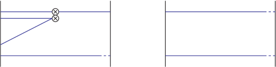
Finally, we define the ratios

$${\cal A}_{k;s,\alpha}=\frac{F_{k;s}(T/2)}{f_{1}^{\scriptscriptstyle{\frac{3}{2}}-\alpha}k_{1}^{\alpha}}\,,$$ (3.84)

where $\alpha$ is an arbitrary real parameter. The structure of $F_{k;s}$ and $f_{1},k_{1}$ is illustrated in Fig. 1.

Figure 1: Feynman diagrams for the four-quark correlation functions $F_{k;s}$ and the boundary-to-boundary correlators $f_{1},k_{1}$ at tree level. Euclidean time goes from left to right. The double blob indicates the four-quark operator insertion, and dashed lines indicate the explicit time-like link variable involved in boundary-to-boundary quark propagators.

We then proceed to impose renormalisation conditions at bare coupling $g_{0}$ and scale $\mu=1/L$ by generalising the condition introduced in [28, 29] for the renormalisable multiplicative operators ${\cal Q}_{1}^{\pm}$: the latter reads

$$\mathcal{Z}_{11;s,\alpha}\,{\cal A}_{1;s,\alpha}=\left.{\cal A}_{1;s,\alpha}\right|_{g_{0}^{2}=0}\,,$$ (3.85)

while for operators that mix in doublets, we impose

$$\left(\begin{array}[]{cc}\mathcal{Z}_{22;s_{1},s_{2},\alpha}&\mathcal{Z}_{23;s_{1},s_{2},\alpha}\\ \mathcal{Z}_{32;s_{1},s_{2},\alpha}&\mathcal{Z}_{33;s_{1},s_{2},\alpha}\\ \end{array}\right)\left(\begin{array}[]{cc}{\cal A}_{2;s_{1},\alpha}&{\cal A}_{2;s_{2},\alpha}\\ {\cal A}_{3;s_{1},\alpha}&{\cal A}_{3;s_{2},\alpha}\\ \end{array}\right)=\left(\begin{array}[]{cc}{\cal A}_{2;s_{1},\alpha}&{\cal A}_{2;s_{2},\alpha}\\ {\cal A}_{3;s_{1},\alpha}&{\cal A}_{3;s_{2},\alpha}\\ \end{array}\right)_{g_{0}^{2}=0}\,,$$ (3.92)

and similarly for ${\cal Q}_{4,5}$. The products of boundary-to-boundary correlators in the denominator of Eq. (3.84) cancels the renormalisation of the boundary operators in $F_{k;s}$, and therefore $\mathcal{Z}_{k;s,\alpha}$ only contains anomalous dimensions of four-fermion operators. Following [23, 28, 31], conditions are imposed on renormalisation functions evaluated at $x_{0}=T/2$, and the phase that parameterises spatial boundary conditions on fermion fields is fixed to $\theta=0.5$. Together with the $L=T$ geometry of our finite box, this fixes the renormalisation scheme completely, up to the choice of boundary source, indicated by the index $s$, and the parameter $\alpha$. The latter can in principle take any value, but we will restrict to the choices $\alpha=0,1,3/2$.

One still has to check that renormalisation conditions are well-defined at tree-level. While this is straightforward for Eq. (3.85), it is not so for Eq. (3.92): it is still possible that the matrix of ratios ${\cal A}$ has zero determinant at tree-level, rendering the system of equations for the matrix of renormalisation constants ill-conditioned. This is indeed the obvious case for $s_{1}=s_{2}$, but the determinant turns out to be zero also for other non-trivial choices $s_{1}\neq s_{2}$. In practice, out of the ten possible schemes one is only left with six, viz.

$$(s_{1},s_{2})\in\{(1,2),(1,4),(1,5),(2,3),(3,4),(3,5)\}\,.$$ (3.93)

It has to be stressed that this property is independent of the choice of $\theta$ and $\alpha$. Thus, we are left with a total of 15 schemes for ${\cal Q}_{1}^{\pm}$, and 18 for each of the pairs $({\cal Q}_{2}^{\pm},{\cal Q}_{3}^{\pm})$ and $({\cal Q}_{4}^{\pm},{\cal Q}_{5}^{\pm})$.

3.4 One-loop results in the SF

Let us now carry out a perturbative computation of the SF renormalisation matrices introduced above, using a lattice regulator. For any of the correlation functions discussed in Section 3, the perturbative expansion reads

$$X=X^{(0)}+g_{0}^{2}\left[X^{(1)}+m_{\rm cr}^{(1)}\frac{\partial X^{(0)}}{\partial m_{0}}\right]+{\cal O}(g_{0}^{4})\,,$$ (3.94)

where $X$ is one of $F_{k;s}^{\pm}(x_{0}),~{}f_{1},~{}k_{1}$, or some combination thereof; where $m_{0}$ is the bare quark mass; and $m_{\rm cr}^{(1)}$ the one-loop coefficient in the perturbative expansion of the critical mass. The derivative term in the square bracket is needed to set the correlation function $X$ to zero renormalised quark mass, when every term in the r.h.s. of the equation is computed at vanishing bare mass. We use the values for the critical mass provided in [35],

$$\begin{split}m_{\rm cr}^{(1)}&=-0.20255651209\,C_{\rm F}~{}~{}~{}(c_{\rm sw}=1)\,,\\ m_{\rm cr}^{(1)}&=-0.32571411742\,C_{\rm F}~{}~{}~{}(c_{\rm sw}=0)\,,\end{split}$$ (3.95)

with $C_{\rm F}=(N^{2}-1)/(2N)$, and the (tree-level) value of the Sheikholeslami-Wohlert (SW) coefficient $c_{\rm sw}$ indicating whether the computation is performed with or without an $\mbox{O}(a)$-improved action.

The entries of the renormalisation matrix admit a similar expansion,

$$\mathcal{Z}(g_{0},L/a)=1+g_{0}^{2}\mathcal{Z}^{(1)}(L/a)+{\cal O}(g_{0}^{4})\,,$$ (3.96)

where we have indicated explicitly the dependence of the quantities on the bare coupling and the lattice spacing-rescaled renormalisation scale $a\mu=a/L$. The explicit expression of the one-loop order coefficient $\mathcal{Z}^{(1)}$ for the multiplicatively renormalisable operators ${\cal Q}_{1}^{\pm}$ is

$$\begin{split}\mathcal{Z}^{(1)}&=-\left\{\frac{F^{(1)}}{F^{(0)}}+\frac{F^{(1)}_{b}}{F^{(0)}}+m_{\rm cr}^{(1)}\frac{\partial}{\partial m_{0}}\log F^{(0)}\right\}\\ &+\left(\frac{3}{2}-\alpha\right)\left[\frac{f_{1}^{(1)}}{f_{1}^{(0)}}+\frac{f_{1;b}^{(1)}}{f_{1}^{(0)}}+m_{\rm cr}^{(1)}\frac{\partial}{\partial m_{0}}\log f_{1}^{(0)}\right]\\ &+\alpha\left[\frac{k_{1}^{(1)}}{k_{1}^{(0)}}+\frac{k_{1;b}^{(1)}}{k_{1}^{(0)}}+m_{\rm cr}^{(1)}\frac{\partial}{\partial m_{0}}\log k_{1}^{(0)}\right]\,,\end{split}$$ (3.97)

while for the entries of each $2\times 2$ submatrix that renormalises operator pairs one has

$$\mathcal{Z}_{ij}^{(1)}=-{\cal A}_{ik}^{(1)}\left[\left({\cal A}^{(0)}\right)^{-1}\right]_{kj}\,,$$ (3.98)

with

$$\begin{split}{\cal A}_{ij}^{(0)}=&\frac{F_{ij}^{(0)}}{\left[f_{1}^{(0)}\right]^{3/2-\alpha}\left[k_{1}^{(0)}\right]^{\alpha}}\,,\\ {\cal A}_{ij}^{(1)}=&\left\{\left[F_{ij}^{(1)}+F_{ij;b}^{(1)}+m_{\rm cr}^{(1)}\frac{\partial}{\partial m_{0}}F_{ij}^{(0)}\right]\right.\\ &-\left(\frac{3}{2}-\alpha\right)\left[\frac{f_{1}^{(1)}}{f_{1}^{(0)}}+\frac{f_{1;b}^{(1)}}{f_{1}^{(0)}}+m_{\rm cr}^{(1)}\frac{\partial}{\partial m_{0}}\log f_{1}^{(0)}\right]F_{ij}^{(0)}\\ &-\alpha\left.\left[\frac{k_{1}^{(1)}}{k_{1}^{(0)}}+\frac{k_{1;b}^{(1)}}{k_{1}^{(0)}}+m_{\rm cr}^{(1)}\frac{\partial}{\partial m_{0}}\log k_{1}^{(0)}\right]F_{ij}^{(0)}\right\}\left[f_{1}^{(0)}\right]^{\alpha-3/2}\left[k_{1}^{(0)}\right]^{-\alpha}\,.\end{split}$$ (3.99)

Contributions with the label “b” arise from the boundary terms that are needed in addition to the SW term in order to achieve full $\mbox{O}(a)$ improvement of the action in the SF [33]. They obviously vanish in the unimproved case. We will set them to zero in the improved case as well, since they vanish in the continuum limit and thus will not contribute to our results for NLO anomalous dimensions.

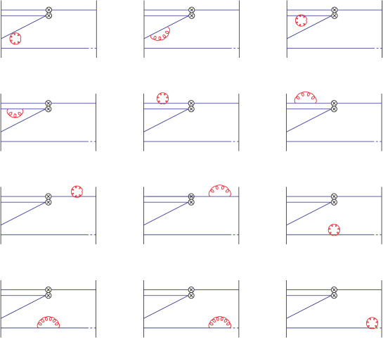
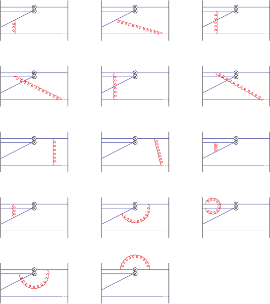
The computation of the r.h.s. of the four-quark operator correlators $F_{k;s}^{\pm}$ requires the evaluation of the Feynman diagrams in Figure 1 at tree level, and of those in Figures 2 and 3 at one loop. The one-loop expansion of the boundary-to-boundary correlators $f_{1}$ and $k_{1}$ is meanwhile known from [36]. Each diagram can be written as a loop sum of a Dirac trace in time-momentum representation, where the Fourier transform is taken over space only. The sums have been performed numerically in double precision arithmetics using a Fortran 90 code, for all even lattice sizes ranging from $L/a=4$ to $L/a=48$. The results have been cross-checked against those of an independent C++ code, also employing double precision arithmetics.

The expected asymptotic expansion for the one-loop coefficient of renormalisation constants is (operator and scheme indices not explicit)

$$\mathcal{Z}^{(1)}(L/a)=\sum_{n=0}^{\infty}\left(\frac{a}{L}\right)^{n}\left\{r_{n}+s_{n}\,\ln(L/a)\right\}\,.$$ (3.100)

In particular, the coefficient $s_{0}$ of the log that survives the continuum limit will be the corresponding entry of the anomalous dimension matrix, while the finite part $r_{0}$ will contribute to the one-loop matching coefficients we are interested in. In particular, one has

$$[{\cal X}_{O}^{(1)}]_{\rm SF;lat}=r_{0}\,,$$ (3.101)

which is the required input for the matching condition in Eq. (3.70). We thus proceed as follows:

1. Compute tree-level and one-loop diagrams for all correlation functions.

2. Construct one-loop renormalisation constants using Eq. (3.97) and Eq. (3.98).

3. Fit the results to the ansatz in Eq. (3.100) as a function of $(a/L)$, using the known value of the entries of the leading-order anomalous dimension matrix $\gamma^{(0)}$ as fixed parameters, and extract $r_{0}$.

The description of the procedure employed to extract the finite parts as well as our results are provided in Appendix E.

Figure 2: Feynman diagrams of the self-energy type entering the one-loop computation of $F_{k;s}^{\pm}$.

Figure 3: Feynman diagrams with gluon exchanges between quark lines entering the one-loop computation of $F_{k;s}^{\pm}$.

3.5 NLO SF anomalous dimensions

Having collected $[{\cal X}_{O}^{(1)}]_{\rm SF;lat}$, $[{\cal X}_{O}^{(1)}]_{\rm cont;lat}$, $\gamma^{(1);\rm cont}$ and ${\cal X}^{(1)}_{\rm g}$ we have finally been able to compute the matrix $\gamma^{(1);\rm SF}$ for both the “+” and the “-” operator basis and for all the 18 schemes presented in Section 3.3. The results are collected in Appendix F.

We have performed two strong consistency checks of our calculation:

• In our one-loop perturbative computation, we have obtained $[{\cal X}_{O}^{(1)}]_{\rm SF;lat}$ for both $c_{\rm sw}=0$ and $c_{\rm sw}=1$ values. The results for $[{\cal X}_{O}^{(1)}]_{\rm cont;lat}$ are known for generic values of $c_{\rm sw}$. We have thus been able to compute $[{\cal X}_{O}^{(1)}]_{\rm SF;cont}$ for both $c_{\rm sw}=0$ and $c_{\rm sw}=1$ in such a way to check its independence from $c_{\rm sw}$.

• For the “+” operators, we have checked the independence of $\gamma^{(1);\rm SF}$ from the reference scheme used (either the RI-MOM or the ${\overline{\rm MS}}$). This is a strong check of the calculations from the literature of the NLO anomalous dimensions $\gamma^{(1);\rm cont}$ and one-loop matching coefficients $[{\cal X}_{O}^{(1)}]_{\rm cont;lat}$ in both the RI-MOM and ${\overline{\rm MS}}$ scheme.

The resulting values of $\gamma^{(1)}$ exhibit a strong scheme dependence. In order to define a reference scheme for each operator, we have devised a criterion that singles out those schemes with the smallest NLO corrections: given the matrix

$$16\pi^{2}\,\gamma^{(1);\rm SF}\,(\gamma^{(0)})^{-1}\,,$$ (3.102)

we compute the the trace and the determinant of each non-trivial submatrix, and look for the smallest absolute value of both quantities. Remarkably, in all cases (2-3 and 4-5 operator doublets, both in the Fierz $+$ and $-$ sectors) this is satisfied by the scheme given by $s=6,~{}\alpha=3/2$.

4 Renormalisation group running in perturbation theory

In this section we will discuss the perturbative computation of the RG running factor $\tilde{U}(\mu)$ in Eq. (2.55). The main purpose of this exercise is to understand the systematic of perturbative truncation, both in view of our own non-perturbative computation of the RG running factor [37] (which involves a matching to NLO perturbation theory around the electroweak scale), and in order to assess the extensive use of NLO RG running down to hadronic scales in the phenomenological literature. In view of our upcoming publication of a non-perturbative determination of the anomalous dimensions for QCD with $N_{\mathrm{\scriptstyle f}}=2$, the analysis below will be performed for that case; the qualitative conclusions are independent of the precise value of $N_{\mathrm{\scriptstyle f}}$. The scale will be fixed using the value $\Lambda_{\rm\scriptscriptstyle QCD}^{{\overline{\rm MS}};N_{\mathrm{\scriptstyle f}}=2}=310(20)~{}{\rm MeV}$ quoted in [38].

At leading order in perturbation theory the running factor is given by $U_{\rm\scriptscriptstyle LO}$ in Eq. (2.48). Beyond LO, the running factor is given by Eq. (2.49), where $W(\mu)$ satisfies Eq. (2.51). In the computation of $W$, the $\beta$ and the $\gamma$ functions are known only up to 3 loops and 2 loops, respectively. In order to asses the systematic, we will compute the running factor for several approximations that will be labeled through a pair of numbers “$n_{\gamma}/n_{\beta}$” where $n_{\gamma}$ is the order used for the $\gamma$ function while $n_{\beta}$ is the order used for the $\beta$ function. We will consider the following cases:

1. “1/1”, i.e. the LO approximation in which $W\equiv 1$;

2. “2/2”, in which both $\gamma$ and $\beta$ are taken at NLO;

3. “2/3”, in which $\beta$ is taken at NNLO and $\gamma$ at NLO;

4. “+3/3”, in which $\beta$ is taken at NNLO and for the NNLO coefficient $\gamma_{2}$ we use a guesstimate given by $\gamma_{2}\gamma_{1}^{-1}=\gamma_{1}\gamma_{0}^{-1}$;

5. “-3/3”, in which $\beta$ is taken at the NNLO and for the NNLO coefficient $\gamma_{2}$ we use a guesstimate given by $\gamma_{2}\gamma_{1}^{-1}=-\gamma_{1}\gamma_{0}^{-1}$;

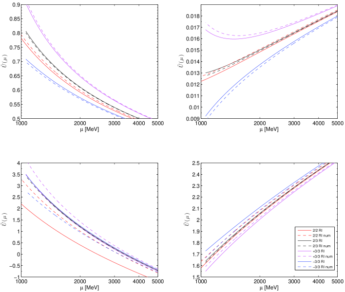
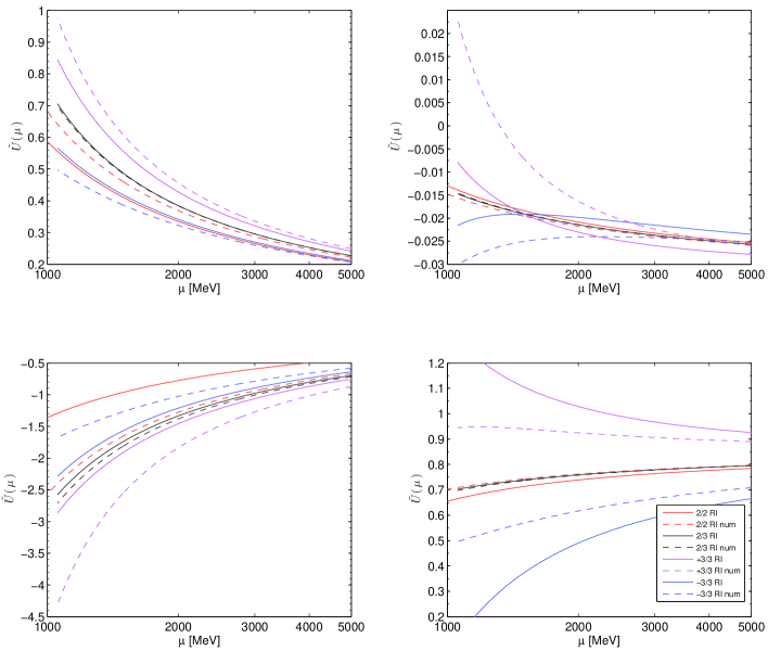
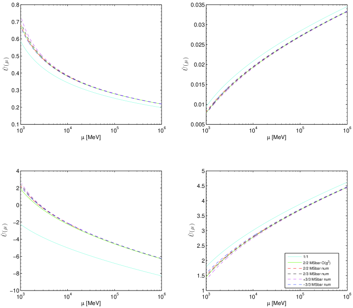
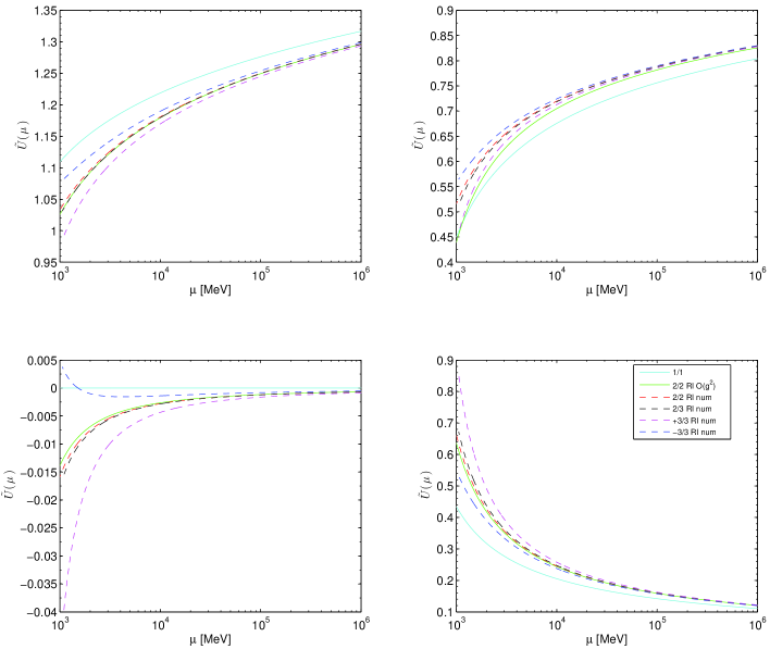
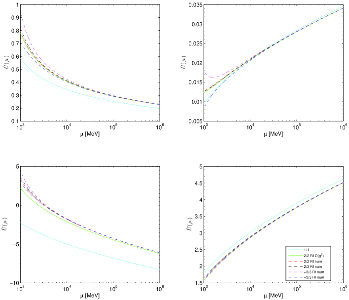
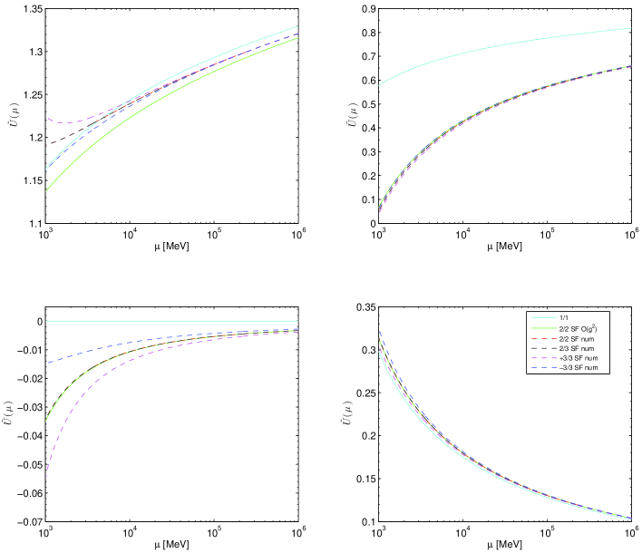
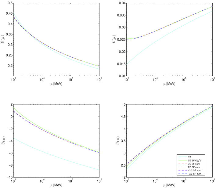
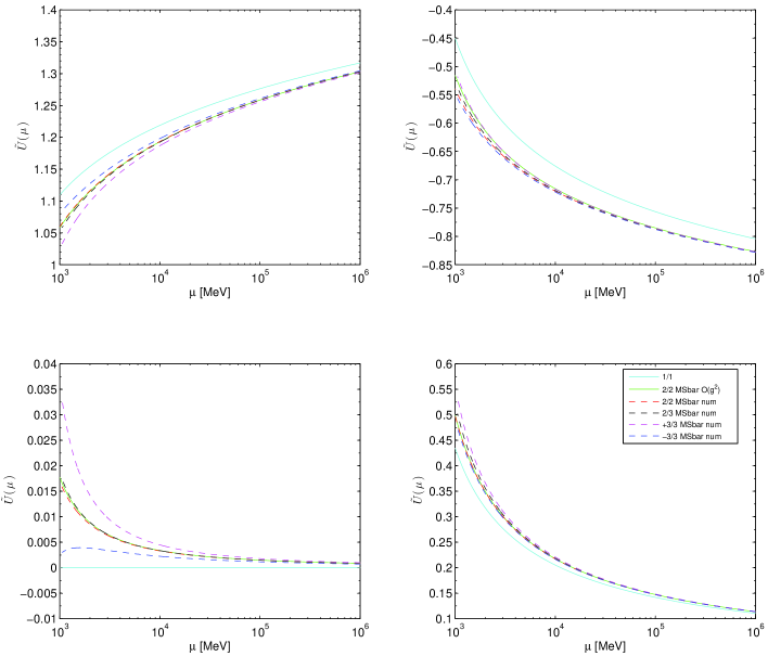
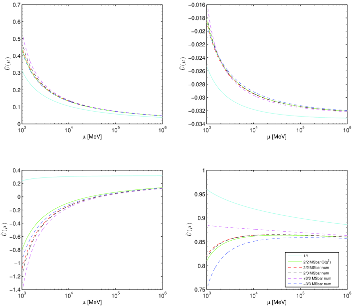
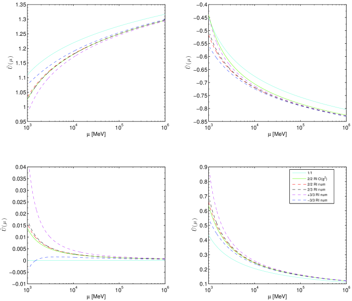
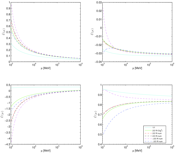
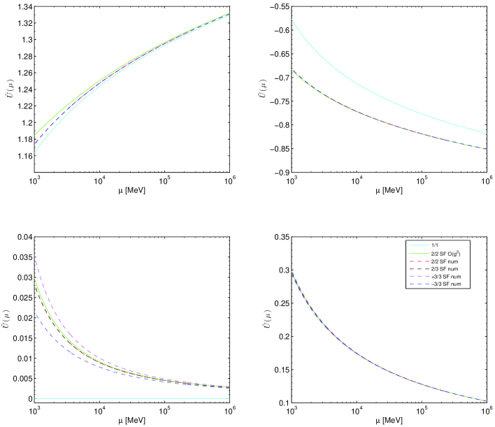
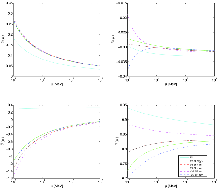
Beyond LO we have first computed the perturbative expansion of the running factor, Eq. (2.49) and Eq. (2.56), by including all the $J_{n}$’s corresponding to the highest order used in the combinations of $\beta$/$\gamma$ functions chosen above. The $J_{n}$ have been computed from Eq. (2.57) and Eq. (2.58) setting the unknown coefficients to zero. Namely: $J_{1}$ in the 2/2 case, $J_{1}$ and $J_{2}$ (with $\gamma_{2}=0$) in the 2/3 case, $J_{1}$ and $J_{2}$ with $\gamma_{2}$ set to the guesstimates above in the +3/3 and -3/3 cases. We have compared these results with the numerical solution of Eq. (2.51) in which the perturbative expansions for $\gamma$ and $\beta$ at the chosen orders are plugged in. We have chosen two cases in which perturbation theory seems particularly ill-behaved, namely the matrix for operators 4 and 5 with both Fierz + and - in the RI-MOM scheme, and we show the comparison in Fig. 4. As one can see, the two methods are not in very good agreement in the region of few GeV scales. This is obvious, because by expanding $W$ in powers of $g^{2}$ and including only the first/second coefficients $J_{1}$, $J_{2}$, substantial information is lost.

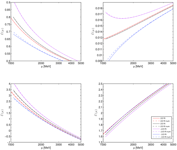
We have then included in the perturbative expansion the next order, computed from Eq. (2.58) and Eq. (2.6), setting again the unknown coefficients to zero. Namely: $J_{2}$ (with $b_{2}=\gamma_{2}=0$) in the 2/2 case, $J_{3}$ (with $b_{3}=\gamma_{3}=\gamma_{2}=0$) in the 2/3 case, $J_{3}$ (with $b_{3}=\gamma_{3}=0$ and $\gamma_{2}$ set to the guesstimates above) in the +3/3 and -3/3 cases. The comparison, again with the corresponding numerical solution of Eq. (2.51) (which remains unchanged), is shown in Fig. 5 and shows a reasonable agreement for the Fierz + matrix while still noticeable desagreement for some of the Fierz - matrix elements.

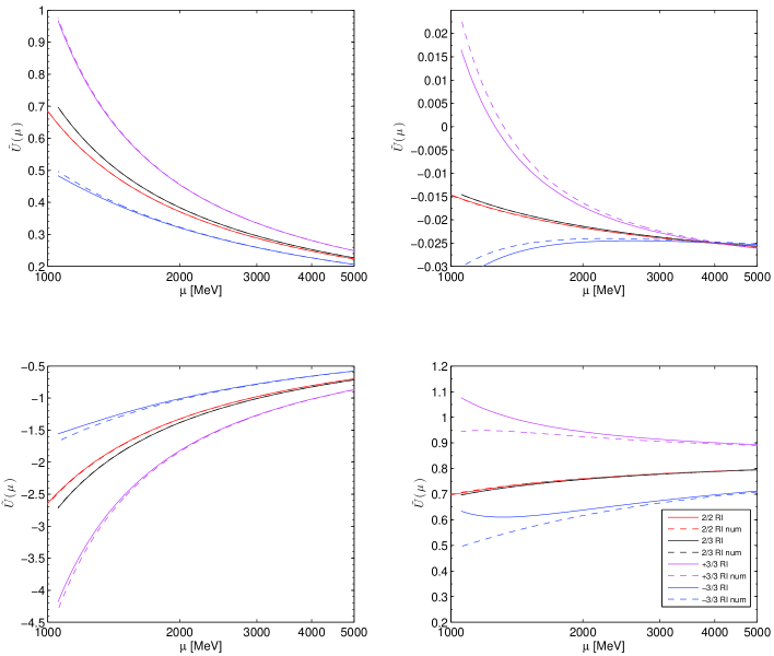
In the the Fierz - case we have thus proceeded by introducing the next order, namely: $J_{3}$ (with $b_{2}=\gamma_{2}=b_{3}=\gamma_{3}=0$) in the 2/2 case, $J_{4}$ (with $b_{4}=b_{3}=\gamma_{4}=\gamma_{3}=\gamma_{2}=0$) in the 2/3 case, $J_{4}$ (with $b_{4}=b_{3}=\gamma_{4}=\gamma_{3}=0$ and $\gamma_{2}$ set to the guesstimates above) in the +3/3 and -3/3 cases. The comparison, again with the corresponding numerical solution of Eq. (2.51), is shown in Fig. 6a. The agreement between the numerical solution and the perturbative expansion further improves in all cases except for the 55 matrix element in the $\pm 3/3$ cases where the perturbative expansion further moves away from the numerical solution. From both examples of Fierz $\pm$ 4-5 matrix, we understand that by including more and more orders in the perturbative expansion of $W(\mu)$ Eq. (2.56), we approximate better and better the numerical solution of Eq. (2.51) , which can thus be considered the best approximation of the running factor given a fixed order computation of the $\beta$ and $\gamma$ functions.

There is still a subtle technical issue concerning the numerical integration of Eq. (2.51) which needs to be discussed, because it becomes relevant in practice. Since $\gamma$ and $\beta$ have simple expressions in terms of $\kern 1.0pt\overline{\kern-1.0ptg\kern 0.0pt}\kern 1.0pt(\mu)$ rather than in terms of $\mu$, Eq. (2.51) is most easily solved by rewriting it in terms of the derivative with respect to the coupling, viz.

$$\widetilde{W}^{\prime}(g)=-\widetilde{W}(g)\,\frac{\gamma(g)}{\beta(g)}+\frac{\gamma_{0}}{b_{0}g}\,\widetilde{W}(g)\,,$$ (4.103)

where $\widetilde{W}(\kern 1.0pt\overline{\kern-1.0ptg\kern 0.0pt}\kern 1.0pt(\mu))\equiv W(\mu)$. While both terms on the right hand side diverge as $g\to 0$, the divergence cancels in the sum due to Eq. (2.52). However, it is not straightforward to implement this latter initial condition at the level of the numerical solution to Eq. (4.103): a stable numerical solution requires fixing the initial condition Eq. (2.52) at an extremely small value of the coupling, and consequently the use of a sophisticated and computationally expensive integrator. A simpler solution is to substitute Eq. (2.52) by an initial condition of the form

$$\widetilde{W}(g_{\rm i})=\mathbf{1}+g_{\rm i}^{2}J_{1}+g_{\rm i}^{4}J_{2}+g_{\rm i}^{6}J_{3}+g_{\rm i}^{8}J_{4}+\ldots\,,$$ (4.104)

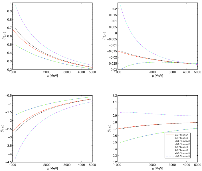
at some very perturbative coupling $g_{\rm i}$ (but still a significantly larger value than required by Eq. (2.52)), where we include exactly the same coefficients $J_{n}$, $n=1,\ldots$ that we use in the perturbative expansion of the running factor, and which are computed by using the same amount of perturbative information employed in the ratio $\gamma/\beta$ used for the numerical integration. Note that indeed the numerical value of $g_{\rm i}$ needs not be extremely small for this to make physical sense, e.g. for $N_{\mathrm{\scriptstyle f}}=2$ (which will be of particular interest to us) and at the Planck scale one has $\kern 1.0pt\overline{\kern-1.0ptg\kern 0.0pt}\kern 1.0pt^{2}_{{\overline{\rm MS}}}(M_{P})\approx 0.221\leftrightarrow\alpha_{\rm s}^{{\overline{\rm MS}}}(M_{P})\approx 0.0176$ and $\kern 1.0pt\overline{\kern-1.0ptg\kern 0.0pt}\kern 1.0pt^{2}_{\rm SF}(M_{P})$ differs with respect to $\kern 1.0pt\overline{\kern-1.0ptg\kern 0.0pt}\kern 1.0pt^{2}_{{\overline{\rm MS}}}(M_{P})$ only on the third decimal digit.

In Fig. 6b we compare the results for the numerical integration of $W(\mu)$ when matched at $g_{\rm i}$ with the perturbative expansion at the order used in Fig. 4 and Fig. 5 respectively and the results turn out to be indistiguishable. We have also changed the value of the coupling chosen for the matching in a broad range of $\kern 1.0pt\overline{\kern-1.0ptg\kern 0.0pt}\kern 1.0pt^{2}$ without observing any noticeable difference in the solution. These checks prove the stability of the numerical procedure and give us confidence in the corresponding results, which will be used below to assess the systematic uncertainties. In the following we won’t consider anymore the perturbative expansion of the running factor except for the 2/2 case where only $J_{1}$ is included (we will call this $2/2$ at $\mbox{O}(g^{2})$), which is the case usually considered in literature, both for phenomenological application and in lattice computations.

Figure 4: RG running matrix for the Op $4,5$ in the RI scheme. Top half (a): Fierz $+$. Bottom half (b): Fierz $-$. The four cases $n_{\gamma}/n_{\beta}=\{2/2,2/3,+3/3,-3/3\}$ are plotted respectively in red, black, magenta and blue. Dashed lines correspond to the numerical integration of $W(\mu)$. Solid lines correspond to the perturbative expansion up to ${\mbox{O}}(g^{2})$ (i.e. $J_{1}$) for the 2/2 case and up to ${\mbox{O}}(g^{4})$ (i.e. $J_{2}$) for the 2/3, $+3/3$ and $-3/3$ cases.

Figure 5: RG running matrix for the Op $4,5$ in the RI scheme. Top half (a): Fierz $+$. Bottom half (b): Fierz $-$. The four cases $n_{\gamma}/n_{\beta}=\{2/2,2/3,+3/3,-3/3\}$ are plotted respectively in red, black, magenta and blue. Dashed lines correspond to the numerical integration of $W(\mu)$. Solid lines correspond to the perturbative expansion up to ${\mbox{O}}(g^{4})$ (i.e. $J_{2}$) for the 2/2 case and up to ${\mbox{O}}(g^{6})$ (i.e. $J_{3}$) for the 2/3, $+3/3$ and $-3/3$ cases.

Figure 6: RG running matrix for the Op $4,5$ Fierz $-$ in the RI scheme. Top half (a): the four cases $n_{\gamma}/n_{\beta}=\{2/2,2/3,+3/3,-3/3\}$ are plotted respectively in red, black, magenta and blue. Dashed lines correspond to the numerical integration of $W(\mu)$. Solid lines correspond to the perturbative expansion up to ${\mbox{O}}(g^{6})$ (i.e. $J_{3}$) for the 2/2 case and up to ${\mbox{O}}(g^{8})$ (i.e. $J_{4}$) for the 2/3, $+3/3$ and $-3/3$ cases. Bottom half (b): comparison of the results for the numerical integration of $W(\mu)$ when matched at $\kern 1.0pt\overline{\kern-1.0ptg\kern 0.0pt}\kern 1.0pt^{2}_{{\overline{\rm MS}}}(M_{P})$ with the perturbative expansion at the order used in Fig. 4 (solid lines) and Fig. 5 (dashed lines).

According to the previous discussion, we have chosen to quote as our best estimate of the running factors the 2/3 results (which encode the maximum of information at our disposal for the $\beta$ and $\gamma$ functions) obtained through numerical integration. They are presented in Tab. 1 at the scale $\mu=3\,{\rm GeV}$. In alternative we quote also the results for the 2/2 case perturbatively expanded at $\mbox{O}(g^{2})$ (i.e. including $J_{1}$ only), which are the results usually considered in literature. We present them in Tab. 2 again at the scale $\mu=3\,{\rm GeV}$.

The systematic uncertainties in Tab. 1 (respectively Tab. 2) are estimated by considering the maximal deviation of the 2/3 case (respectively the 2/2, $\mbox{O}(g^{2})$ case) from the other 3 (respectively 4) numerical cases.

The results for the LO running factor $U_{\rm\scriptscriptstyle LO}(\mu)$ Eq. (2.48) and the numerically integrated $\tilde{U}(\mu)$ running factors beyond LO (ii)-(v) described above are illustrated in Figs. (7), (8), (9), (10), (11), (12) together with the 2/2 $\mbox{O}(g^{2})$ perturbative expansion, for the four doublets of operators and three different schemes (${\overline{\rm MS}}$, RI and a chosen SF scheme).

Some important observations are:

• The convergence of LO respect to NLO and NNLO seems to be slow in all the schemes under investigation for almost all the operators. In particular, for the matrix elements involving tensor current (4-5 sub-matrices) the convergence is very poor. Note that the LO anomalous dimensions for these submatrices are already very large compared with the others.

• the 2/3 numerical running factors have always symmetric systematic errors, because most of the systematics is due to the inclusion of the guesstimate for $\gamma_{2}$ with + and - sign, and these effects turn out to be always symmetric with respect to the 2/3 (and also 2/2) cases.

• the 2/2 $\mbox{O}(g^{2})$ running factors are, for several matrix elements, quite far from the 2/3 (and also the 2/2) numerical ones. Possibly even further away than the $\pm 3/3$ and have thus very large, asymmetric errors.

• For both 4-5 sub-matrices (Fierz + and -) the ratio $\gamma_{1}\gamma_{0}^{-1}$ turns out to have large matrix elements. As a consequence, our plausibility argument for the guesstimates $\gamma_{2}\gamma_{1}^{-1}=\pm\gamma_{1}\gamma_{0}^{-1}$ leads to large systematic uncertainties. In particular, for the 54 matrix element the error is huge in the RI scheme and large also in the ${\overline{\rm MS}}$ and SF schemes, already for the 2/3 numerical solution (for the 2/2 $\mbox{O}(g^{2})$ perturbative expansion the situation is much worse). This obviously poses serious doubts on all the computations of $\Delta F=2$ matrix elements beyond the Standard Model which uses perturbative running (in all cases through the 2/2 $\mbox{O}(g^{2})$ expansion) down to scales of 3 ${\rm GeV}$ or less.

5 Conclusions

In this paper we have reviewed the renormalisation and RG running properties of the four-quark operators relevant for BSM analyses, and introduced a family of SF schemes that allow to compute them in a fully non-perturbative way. Our non-perturbative results for $N_{\mathrm{\scriptstyle f}}=2$ QCD will be presented in a separate publication [39]. Here we have focused on the perturbative matching of our schemes to commonly used perturbative schemes and to RGI operators. One of our main results in this context is the full set of NLO operator anomalous dimensions in our SF schemes.

We have also conducted a detailed analysis of perturbative truncation effects in operator RG running in both the SF schemes introduced here, and in commonly used ${\overline{\rm MS}}$ and RI-MOM schemes. We conclude that when NLO perturbation theory is used to run the operators from high-energy scales down to the few GeV range, large truncation effects appear. One striking example is the mixing of tensor-tensor and scalar-scalar operators, where all the available indications point to extremely large anomalous dimensions and very poor perturbative convergence. One important point worth stressing is that, in the computation of the running factor $W(\mu)$, the use of the truncated perturbative expansion in Eq. (2.56) leads to a significantly worse behaviour than the numerical integration of Eq. (2.51) with the highest available orders for $\gamma$ and $\beta$.

A context where these findings might have an important impact is e.g. the computation of BSM contributions to neutral kaon mixing. At present, few computations of the relevant $\Delta S=2$ operators exist with dynamical fermions [41, 42, 43, 44, 45], all of which use perturbative RG running (and, in the case of [44], perturbative operator renormalisation as well). There are substantial discrepancies between the various results in [41, 42, 43, 44, 45], which may be speculated to stem, at least in part, from perturbative truncation effects. Another possible contribution to the discrepancy is the delicate pole subtraction required in the RI-MOM scheme — indeed, results involving perturbative renormalisation and non-perturbative renormalisation constants in RI-SMOM schemes are consistent. At any rate, future efforts to settle this issue, as well as similar studies for $\Delta B=2$ amplitudes, should put a strong focus on non-perturbative renormalisation.

A Constraints on anomalous dimensions from chiral symmetry

In section 5.3 of [1] the authors derive an identity between the the renormalisation matrices for $({\cal Q}_{2}^{+},{\cal Q}_{3}^{+})$ and $({\cal Q}_{2}^{-},{\cal Q}_{3}^{-})$, valid in the RI-MOM scheme considered in that paper. Here we discuss how such an identity can be derived from generic considerations based on chiral symmetry, and how (or, rather, under which conditions) it can be generalised to other renormalisation schemes.

Let us consider a renormalised matrix element of the form $\langle f|\bar{Q}_{k}^{\pm}|i\rangle$, where $Q_{k}^{\pm}$ is a parity-even operator and $|i,f\rangle$ are stable hadron states with the same, well-defined parity. Simple examples would be the matrix elements of $\Delta F=2$ operators providing the hadronic contribution to $K^{0}$–$\bar{K}^{0}$ or $B^{0}$–$\bar{B}^{0}$ oscillation amplitudes (cf. Section 2). Bare matrix elements can be extracted from suitable three-point Euclidean correlation functions

$$\langle{\cal O}_{f}(x)\,Q_{k}^{\pm}(0)\,{\cal O}_{i}(y)\rangle=\frac{1}{{\cal Z}}\int D[\psi]D[\bar{\psi}]D[A]\,e^{-S}\,{\cal O}_{f}(x)\,Q_{k}^{\pm}(0)\,{\cal O}_{i}(y)$$ (A.105)

where ${\cal O}_{i,f}$ are interpolating operators for the external states $|i,f\rangle$. If we perform a change of fermion variables of the form

$$\psi\to\psi^{\prime}=e^{i\gamma_{5}T}\psi\,,~{}~{}~{}~{}~{}\bar{\psi}\to\bar{\psi}^{\prime}=\bar{\psi}e^{i\gamma_{5}T}\,,$$ (A.106)

where $\psi$ is a fermion field with $N_{\mathrm{\scriptstyle f}}$ flavour components and $T$ is a traceless matrix acting on flavour space, this will induce a corresponding transformation $Q_{k}^{\pm}\to{Q_{k}^{\prime}}^{\pm}$, ${\cal O}_{i,f}\to{\cal O}^{\prime}_{i,f}$ of the involved composite operators. If the regularised theory employed to define the path integral preserves exactly the ${\rm SU}(N_{\mathrm{\scriptstyle f}})_{\rm A}$ axial chiral symmetry of the formal continuum theory, the equality $\langle{\cal O}_{f}(x)\,Q_{k}^{\pm}(0)\,{\cal O}_{i}(y)\rangle=\langle{\cal O}^{\prime}_{f}(x)\,{Q_{k}^{\prime}}^{\pm}(0)\,{\cal O}^{\prime}_{i}(y)\rangle$ will hold exactly; otherwise, it will only hold upon renormalisation and removal of the cutoff. At the level of matrix elements, one will then have

$$\langle f|\bar{Q}_{k}^{\pm}|i\rangle_{(\psi,\bar{\psi})}=\langle f|\bar{Q_{k}^{\prime}}^{\pm}|i\rangle_{(\psi^{\prime},\bar{\psi}^{\prime})}\,,$$ (A.107)

where the subscript remarks that the interpretation of the operator depends on the fermion variables used on each side of the equation. If the flavour matrix $T$ is not traceless, the argument will still hold if the fermion fields entering composite operators are part of a valence sector, employed only for the purpose of defining suitable correlation functions.

The result in Eq. (A.106) is at the basis e.g. of the definition of twisted-mass QCD lattice regularisations, and is discussed in more detail in [2, 3, 4]. Indeed, the rotation in Eq. (A.106) will in general transform the mass term of the action. One crucial remark at this point is that, if a mass-independent renormalisation scheme is used, renormalisation constants for any given composite operator will be independent of which fermion variables are employed in the computation of the matrix element.

Let us now consider a particular case of Eq. (A.106) given by

$$T=\frac{\pi}{4}\left(\begin{array}[]{rrrr}1&0&0&0\\ 0&1&0&0\\ 0&0&1&0\\ 0&0&0&-1\end{array}\right)\,,$$ (A.112)

where $\psi=(\psi_{1},\psi_{2},\psi_{3},\psi_{4})^{T}$ comprises the four, formally distinct flavours that enter $Q_{k}^{\pm},{\cal Q}_{k}^{\pm}$. Under this rotation, the ten operators of the basis in Eq. (2.6) transform as

$$\begin{split}Q_{1}^{\pm}&\to i{\cal Q}_{1}^{\pm}\,,\\ Q_{2}^{\pm}&\to-i{\cal Q}_{2}^{\mp}\,,\\ Q_{3}^{\pm}&\to i{\cal Q}_{3}^{\mp}\,,\\ Q_{4}^{\pm}&\to i{\cal Q}_{4}^{\pm}\,,\\ Q_{5}^{\pm}&\to i{\cal Q}_{5}^{\pm}\,.\end{split}$$ (A.113)

In the case of operators 1,4,5 the rotation is essentially trivial, in that it preserves Fierz ($2\leftrightarrow 4$ exchange) eigenstates. However, in the rotation of operators 2,3 the Fierz eigenvalue is exchanged. One thus has, at the level of renormalised matrix elements,

$$\langle f|\bar{\mathbf{Q}}^{+}(\mu)|i\rangle_{(\psi,\bar{\psi})}=R\langle f|\bar{\boldsymbol{{{\cal Q}}}}^{-}(\mu)|i\rangle_{(\psi^{\prime},\bar{\psi}^{\prime})}\,,$$ (A.114)

where $\mathbf{Q}^{+}=(Q_{2}^{+},Q_{3}^{+})^{T}$, ${\boldsymbol{{{\cal Q}}}}^{-}=({\cal Q}_{2}^{-},{\cal Q}_{3}^{-})^{T}$, and $R=-i\tau^{3}$. In this latter expression we have written explicitly the renormalisation scale $\mu$. If we now use the RG evolution operators discussed in Section 2 to run Eq. (A.114) to another scale $\mu^{\prime}$, one then has (recall that the continuum anomalous dimensions of $Q_{k}^{+}$ and ${\cal Q}_{k}^{+}$ — respectively, $Q_{k}^{-}$ and ${\cal Q}_{k}^{-}$ — are the same)

$$\begin{split}\langle f|\bar{\mathbf{Q}}^{+}(\mu^{\prime})|i\rangle_{(\psi,\bar{\psi})}&=U^{+}(\mu^{\prime},\mu)\langle f|\bar{\mathbf{Q}}^{+}(\mu)|i\rangle_{(\psi,\bar{\psi})}\\ &=U^{+}(\mu^{\prime},\mu)R\langle f|\bar{\boldsymbol{{{\cal Q}}}}^{-}(\mu)|i\rangle_{(\psi^{\prime},\bar{\psi}^{\prime})}\\ &=U^{+}(\mu^{\prime},\mu)R[U^{-}(\mu^{\prime},\mu)]^{-1}\langle f|\bar{\boldsymbol{{{\cal Q}}}}^{-}(\mu^{\prime})|i\rangle_{(\psi^{\prime},\bar{\psi}^{\prime})}\\ &=U^{+}(\mu^{\prime},\mu)R[U^{-}(\mu^{\prime},\mu)]^{-1}R^{-1}\langle f|\bar{\mathbf{Q}}^{+}(\mu^{\prime})|i\rangle_{(\psi,\bar{\psi})}\,,\end{split}$$ (A.115)

which implies

$$U^{+}(\mu^{\prime},\mu)=RU^{-}(\mu^{\prime},\mu)R^{-1}~{}~{}~{}~{}\forall\mu,\mu^{\prime}\,.$$ (A.116)

It is then immediate that the anomalous dimension matrices entering $U^{\pm}$ are related as

$$\gamma^{+}=\left(\begin{array}[]{cc}\gamma_{22}^{+}&\gamma_{23}^{+}\\ \gamma_{32}^{+}&\gamma_{33}^{+}\end{array}\right)=\tau^{3}\gamma^{-}\tau^{3}=\left(\begin{array}[]{cc}\gamma_{22}^{-}&-\gamma_{23}^{-}\\ -\gamma_{32}^{-}&\gamma_{33}^{-}\end{array}\right)\,.$$ (A.121)

The correct interpretation of this identity is that, given an anomalous dimension matrix for, say, $Q_{2,3}^{+}$ and ${\cal Q}_{2,3}^{+}$, one can use Eq. (A.121) to construct a correct anomalous dimension matrix for $Q_{2,3}^{-}$ and ${\cal Q}_{2,3}^{-}$, and vice versa. However, it does not guarantee that, given two different renormalisation conditions for each fierzing, the resulting matrices of anomalous dimensions will satisfy Eq. (A.121). This will only be the case if the renormalisation conditions can be related to each other by the rotation in Eq. (A.112); otherwise, the result of applying Eq. (A.121) to the $\gamma^{-}$ that follows from the condition imposed on Fierz - operators will lead to value of $\gamma^{+}$ in a different renormalisation scheme than the one defined by the renormalisation condition imposed directly on Fierz + operators.

The RI-MOM conditions of [1], as well as typical ${\overline{\rm MS}}$ renormalisation conditions, result in schemes that satisfy the identity directly, since the quantities involved respect the underlying chiral symmetry — e.g. the amputated correlation functions used in RI-MOM rotate in a similar way to the three-point functions discussed above. Indeed, the known NLO anomalous dimensions in RI-MOM and ${\overline{\rm MS}}$ given in Appendix B, as well as (within uncertainties) the non-perturbative values of RI-MOM renormalisation constants, fulfill Eq. (A.121). Our SF renormalisation conditions, on the other hand, are not related among them via rotations with $R$, due to the chiral symmetry-breaking effects induced by the non-trivial boundary conditions imposed on the fields. As a consequence, the finite parts of the matrices of SF renormalisation constants, and hence $\gamma_{2}^{\rm SF}$, do not satisfy the identity. It has to be stressed that, as a consequence of the existence of schemes where Eq. (A.121) is respected, the identity is satisfied by the universal matrices $\gamma_{0}^{\pm}$, as can be readily checked in Eq. (2.39); therefore, the violation of the identity in e.g. SF schemes appears only at ${\cal O}(g_{0}^{4})$ in perturbation theory.

B NLO anomalous dimensions in continuum schemes

The two-loop anomalous dimension matrices in the RI-MOM scheme (in Landau gauge) [5, 8] and ${\overline{\rm MS}}$ scheme [8] are given by (the factor $(4\pi)^{-4}$ has been omitted below to simplify the notation):

$$\begin{split}\gamma^{+,(1);{\rm RI}}_{22}&=\frac{(297+16\log(2))N^{2}+45}{6N^{2}}-N_{f}\frac{2(15+4\log(2))}{3N}\,,\\ \gamma^{+,(1);{\rm RI}}_{23}&=\frac{2\left(4N^{2}(45+2\log(2))-9\right)}{3N}-N_{f}\frac{4}{3}(15+4\log(2))\,,\\ \gamma^{+,(1);{\rm RI}}_{32}&=\frac{(53+160\log(2))N^{2}+108}{12N}-N_{f}\frac{2}{3}(1+2\log(2))\,,\\ \gamma^{+,(1);{\rm RI}}_{33}&=\frac{-379N^{4}+5(99+32\log(2))N^{2}+45}{6N^{2}}+N_{f}\frac{2\left(13N^{2}-4\log(2)-15\right)}{3N}\,,\\ \gamma^{+,(1);{\rm RI}}_{44}&=\frac{-379N^{4}+2(261-88\log(2))N^{3}+140(3+2\log(2))N^{2}-4(-6+60\log(2))N-81}{6N^{2}}+\\ &+\,N_{f}\frac{2\left(13N^{2}+(-15+8\log(2))N-4\log(2)-15\right)}{3N}\,,\\ \gamma^{+,(1);{\rm RI}}_{45}&=\frac{(157-368\log(2))N^{3}+(-494+556\log(2))N^{2}-4(-39+30\log(2))N-72}{36N^{2}}+\\ &+\,N_{f}\frac{((-11+16\log(2))N-20\log(2)+28)}{18N}\,,\\ \gamma^{+,(1);{\rm RI}}_{54}&=\frac{4\left((-165+16\log(2))N^{3}+(-230+76\log(2))N^{2}-4(-39+30\log(2))N-72\right)}{3N^{2}}+\\ &+\,N_{f}\frac{8((15+16\log(2))N-20\log(2)+28)}{3N}\,,\\ \gamma^{+,(1);{\rm RI}}_{55}&=\frac{343N^{4}-2(-343+616\log(2))N^{3}+4(-95+142\log(2))N^{2}+(504+720\log(2))N-531}{18N^{2}}+\\ &-\,N_{f}\frac{2\left(13N^{2}+(41-56\log(2))N+52\log(2)-11\right)}{9N}\,.\end{split}$$

$$\begin{split}\gamma^{-,(1);{\rm RI}}_{22}&=\frac{15}{2N^{2}}+\frac{8\log(2)}{3}+\frac{99}{2}-N_{f}\frac{2(15+4\log(2))}{3N}\,,\\ \gamma^{-,(1);{\rm RI}}_{23}&=-\frac{8}{3}(45+2\log(2))N+\frac{6}{N}+N_{f}\frac{4}{3}(15+4\log(2))\,,\\ \gamma^{-,(1);{\rm RI}}_{32}&=-\frac{1}{12}(53+160\log(2))N-\frac{9}{N}+N_{f}\frac{2}{3}(1+2\log(2))\,,\\ \gamma^{-,(1);{\rm RI}}_{33}&=\frac{-379N^{4}+5(99+32\log(2))N^{2}+45}{6N^{2}}+N_{f}\frac{2\left(13N^{2}-4\log(2)-15\right)}{3N}\,,\\ \gamma^{-,(1);{\rm RI}}_{44}&=\frac{-379N^{4}+2(-261+88\log(2))N^{3}+140(3+2\log(2))N^{2}+24(-1+10\log(2))N-81}{6N^{2}}+\\ &+\,N_{f}\frac{2\left(13N^{2}-(-15+8\log(2))N-4\log(2)-15\right)}{3N}\,,\\ \gamma^{-,(1);{\rm RI}}_{45}&=\frac{(-157+368\log(2))N^{3}+(-494+556\log(2))N^{2}+12(-13+10\log(2))N-72}{36N^{2}}+\\ &-\,N_{f}\frac{((-11+16\log(2))N+20\log(2)-28)}{18N}\,,\\ \gamma^{-,(1);{\rm RI}}_{54}&=-\frac{4\left((-165+16\log(2))N^{3}+(230-76\log(2))N^{2}+(156-120\log(2))N+72\right)}{3N^{2}}+\\ &-\,N_{f}\frac{8((15+16\log(2))N+4(-7+5\log(2)))}{3N}\,,\\ \gamma^{-,(1);{\rm RI}}_{55}&=\frac{343N^{4}+14(-49+88\log(2))N^{3}+4(-95+142\log(2))N^{2}-72(7+10\log(2))N-531}{18N^{2}}+\\ &-\,N_{f}\frac{2\left(13N^{2}+(-41+56\log(2))N+52\log(2)-11\right)}{9N}\,.\end{split}$$

$$\begin{split}\gamma^{+,(1);{{\overline{\rm MS}}}}_{22}&=\frac{15}{2N^{2}}+\frac{137}{6}-N_{f}\frac{22}{3N}\,,\\ \gamma^{+,(1);{{\overline{\rm MS}}}}_{23}&=\frac{200N}{3}-\frac{6}{N}-N_{f}\frac{44}{3}\,,\\ \gamma^{+,(1);{{\overline{\rm MS}}}}_{32}&=\frac{71N}{4}+\frac{9}{N}-N_{f}2\,,\\ \gamma^{+,(1);{{\overline{\rm MS}}}}_{33}&=-\frac{203N^{2}}{6}+\frac{479}{6}+\frac{15}{2N^{2}}+N_{f}\left(\frac{10N}{3}-\frac{22}{3N}\right)\,,\\ \gamma^{+,(1);{{\overline{\rm MS}}}}_{44}&=-\frac{203N^{2}}{6}+\frac{107N}{3}+\frac{136}{3}-\frac{12}{N}-\frac{107}{2N^{2}}+N_{f}\left(\frac{10N}{3}-\frac{2}{3}-\frac{10}{3N}\right)\,,\\ \gamma^{+,(1);{{\overline{\rm MS}}}}_{45}&=-\frac{N}{36}-\frac{31}{9}+\frac{9}{N}-\frac{4}{N^{2}}+N_{f}\left(\frac{1}{9N}-\frac{1}{18}\right)\,,\\ \gamma^{+,(1);{{\overline{\rm MS}}}}_{54}&=-\frac{364N}{3}-\frac{704}{3}-\frac{208}{N}-\frac{320}{N^{2}}+N_{f}\left(\frac{136}{3}+\frac{176}{3N}\right)\,,\\ \gamma^{+,(1);{{\overline{\rm MS}}}}_{55}&=\frac{343N^{2}}{18}+21N-\frac{188}{9}+\frac{44}{N}+\frac{21}{2N^{2}}+N_{f}\left(-\frac{26N}{9}-6+\frac{2}{9N}\right)\,.\end{split}$$

$$\begin{split}\gamma^{-,(1);{{\overline{\rm MS}}}}_{22}&=\frac{15}{2N^{2}}+\frac{137}{6}-N_{f}\frac{22}{3N}\,,\\ \gamma^{-,(1);{{\overline{\rm MS}}}}_{23}&=-\frac{200N}{3}+\frac{6}{N}+N_{f}\frac{44}{3}\,,\\ \gamma^{-,(1);{{\overline{\rm MS}}}}_{32}&=-\frac{71N}{4}-\frac{9}{N}+N_{f}2\,,\\ \gamma^{-,(1);{{\overline{\rm MS}}}}_{33}&=-\frac{203N^{2}}{6}+\frac{479}{6}+\frac{15}{2N^{2}}+N_{f}\left(\frac{10N}{3}-\frac{22}{3N}\right)\,,\\ \gamma^{-,(1);{{\overline{\rm MS}}}}_{44}&=-\frac{203N^{2}}{6}-\frac{107N}{3}+\frac{136}{3}+\frac{12}{N}-\frac{107}{2N^{2}}+N_{f}\left(\frac{10N}{3}+\frac{2}{3}-\frac{10}{3N}\right)\,,\\ \gamma^{-,(1);{{\overline{\rm MS}}}}_{45}&=\frac{N}{36}-\frac{31}{9}-\frac{9}{N}-\frac{4}{N^{2}}+N_{f}\left(\frac{1}{18}+\frac{1}{9N}\right)\,,\\ \gamma^{-,(1);{{\overline{\rm MS}}}}_{54}&=\frac{364N}{3}-\frac{704}{3}+\frac{208}{N}-\frac{320}{N^{2}}+N_{f}\left(\frac{176}{3N}-\frac{136}{3}\right)\,,\\ \gamma^{-,(1);{{\overline{\rm MS}}}}_{55}&=\frac{343N^{2}}{18}-21N-\frac{188}{9}-\frac{44}{N}+\frac{21}{2N^{2}}+N_{f}\left(-\frac{26N}{9}+6+\frac{2}{9N}\right)\,.\end{split}$$

C Perturbative expansion of RG evolution for $N_{\mathrm{\scriptstyle f}}=3$

It is well-known that the condition in Eq. (2.57) that determines the leading non-trivial coefficient in the NLO perturbative expansion of the RG evolution operator, Eq. (2.56), is ill-behaved for the operators $Q_{2,3}^{\pm}$ for $N_{\mathrm{\scriptstyle f}}=30$ and, more relevantly, for $N_{\mathrm{\scriptstyle f}}=3$ [46, 47]. The reason is that, when Eq. (2.57) is written as a linear system, the $4\times 4$ matrix that multiplies the vector of elements of $J_{1}$ has zero determinant, rendering the system indeterminate.

A simple way to understand the anatomy of this problem in greater detail proceeds by writing the explicit solution to Eq. (2.57) as a function of the parameter $\epsilon=3-N_{\mathrm{\scriptstyle f}}$; if the NLO anomalous dimension matrix in the scheme under consideration is written as

$$\gamma_{1}^{\pm}=\frac{1}{(4\pi)^{4}}\left(\begin{array}[]{cc}g_{22}^{\pm}&g_{23}^{\pm}\\ g_{32}^{\pm}&g_{33}^{\pm}\\ \end{array}\right)$$ (C.124)

then one finds

$$J_{1}^{\pm}=\frac{1}{\epsilon}\,J_{1,-1}^{\pm}+J_{1,0}^{\pm}+\epsilon J_{1,1}^{\pm}+{\cal O}(\epsilon^{2})\,,$$ (C.125)

with

$$J_{1,-1}^{\pm} =\frac{1}{(4\pi)^{2}}\left(\begin{array}[]{cc}0&\pm\frac{1}{2}(g_{22}^{\pm}-g_{33}^{\pm})-\frac{3}{4}g_{23}^{\pm}+\frac{1}{3}g_{32}^{\pm}\\[4.30554pt] 0&0\end{array}\right)\,,$$ (C.128)

$$J_{1,0}^{\pm} =\frac{1}{(4\pi)^{2}}\left(\begin{array}[]{cc}\frac{1}{162}(128-9g_{22}^{\pm}\mp 3g_{32}^{\pm})&\frac{1}{27}(\pm 128\mp g_{22}^{\pm}-g_{32}^{\pm}\pm g_{33}^{\pm})\\[4.30554pt] -\frac{1}{36}g_{32}^{\pm}&\frac{1}{162}(-1024\pm 3g_{32}^{\pm}-9g_{33}^{\pm})\\ \end{array}\right)\,,$$ (C.131)

$$J_{1,1}^{\pm} =\frac{1}{(4\pi)^{2}}\left(\begin{array}[]{cc}\frac{1}{4374}(172+18g_{22}^{\pm}\pm 9g_{32}^{\pm})&\pm\frac{1}{2187}(516+6g_{22}^{\pm}\pm 7g_{32}^{\pm}-6g_{33}^{\pm})\\[4.30554pt] \frac{1}{972}g_{32}^{\pm}&\frac{1}{4374}(-1376\mp 9g_{32}^{\pm}+18g_{33}^{\pm})\\ \end{array}\right)\,.$$ (C.134)

In the limit $\epsilon\to 0$ the element $23$ of $J_{1}^{\pm}$ diverges; it is easy to check that the aforementioned $4\times 4$ matrix, consistently, has determinant $\propto\epsilon$. A similar expansion of the matrices $\tilde{U}_{\rm\scriptscriptstyle LO}^{\pm}(\mu)\equiv[\alpha_{\rm\scriptscriptstyle s}(\mu)]^{-\frac{\gamma_{0}^{\pm}}{2b_{0}}}$ yields

$$\tilde{U}_{\rm\scriptscriptstyle LO}^{\pm}(\mu)=\tilde{U}_{\rm\scriptscriptstyle LO,0}^{\pm}(\mu)+\epsilon\tilde{U}_{\rm\scriptscriptstyle LO,1}^{\pm}(\mu)+{\cal O}(\epsilon^{2})\,,$$ (C.135)

with

$$\tilde{U}_{\rm\scriptscriptstyle LO,0}^{\pm}(\mu) =\left(\begin{array}[]{cc}\alpha_{\rm\scriptscriptstyle s}^{-1/9}(\mu)&\mp\frac{2}{3}[\alpha_{\rm\scriptscriptstyle s}^{8/9}(\mu)-\alpha_{\rm\scriptscriptstyle s}^{-1/9}(\mu)]\\[4.30554pt] 0&\alpha_{\rm\scriptscriptstyle s}^{8/9}(\mu)\\ \end{array}\right)\,,$$ (C.138)

$$\tilde{U}_{\rm\scriptscriptstyle LO,1}^{\pm}(\mu) =\left(\begin{array}[]{cc}\frac{2}{243}\alpha_{\rm\scriptscriptstyle s}^{-1/9}(\mu)&\pm\frac{4}{729}[8\alpha_{\rm\scriptscriptstyle s}^{8/9}(\mu)+\alpha_{\rm\scriptscriptstyle s}^{-1/9}(\mu)]\\[4.30554pt] 0&-\frac{16}{243}\alpha_{\rm\scriptscriptstyle s}^{8/9}(\mu)\\ \end{array}\right)\log[\alpha_{\rm\scriptscriptstyle s}(\mu)]\,.$$ (C.141)

When these expressions are plugged in Eq. (2.49), and the perturbative expansion Eq. (2.56) is used, one gets

$$\begin{split}\tilde{U}^{\pm}(\mu)=&~{}\tilde{U}_{\rm\scriptscriptstyle LO,0}^{\pm}(\mu)+\kern 1.0pt\overline{\kern-1.0ptg\kern 0.0pt}\kern 1.0pt^{2}(\mu)\left[\frac{1}{\epsilon}\tilde{U}_{\rm\scriptscriptstyle LO,0}^{\pm}(\mu)J_{1,-1}^{\pm}+\tilde{U}_{\rm\scriptscriptstyle LO,0}^{\pm}(\mu)J_{1,0}^{\pm}+\tilde{U}_{\rm\scriptscriptstyle LO,1}^{\pm}(\mu)J_{1,-1}^{\pm}+{\cal O}(\epsilon)\right]\\ &~{}+{\cal O}(\kern 1.0pt\overline{\kern-1.0ptg\kern 0.0pt}\kern 1.0pt^{4}(\mu))\,,\end{split}$$ (C.142)

which is still divergent as $\epsilon\to 0$. This implies, in particular, that RGI operators cannot be defined consistently using the above form of the perturbative expansion for $W$. The RG evolution operator $U(\mu_{2},\mu_{1})=[\tilde{U}(\mu_{2})]^{-1}\tilde{U}(\mu_{1})$, on the other hand, is finite: the divergent part has the form

$$\frac{1}{\epsilon}\left\{\kern 1.0pt\overline{\kern-1.0ptg\kern 0.0pt}\kern 1.0pt^{2}(\mu_{1})U_{\rm\scriptscriptstyle LO}^{\pm}(\mu_{2},\mu_{1})J_{1,-1}^{\pm}-\kern 1.0pt\overline{\kern-1.0ptg\kern 0.0pt}\kern 1.0pt^{2}(\mu_{2})J_{1,-1}^{\pm}U_{\rm\scriptscriptstyle LO}^{\pm}(\mu_{2},\mu_{1})\right\}=\frac{\pm\frac{1}{2}(g_{22}^{\pm}-g_{33}^{\pm})-\frac{3}{4}g_{23}^{\pm}+\frac{1}{3}g_{32}^{\pm}}{4\pi\epsilon}\,M\,,$$ (C.143)

with

$$M=U_{\rm\scriptscriptstyle LO}^{\pm}(\mu_{2},\mu_{1})\left(\begin{array}[]{cc}0&\alpha_{\rm\scriptscriptstyle s}(\mu_{2})\\ 0&0\end{array}\right)-\left(\begin{array}[]{cc}0&\alpha_{\rm\scriptscriptstyle s}(\mu_{1})\\ 0&0\end{array}\right)U_{\rm\scriptscriptstyle LO}^{\pm}(\mu_{2},\mu_{1})\,,$$ (C.148)

and it is easy to check, using the explicit expression for $\tilde{U}_{\rm\scriptscriptstyle LO,0}^{\pm}(\mu)$ and the identity $U_{\rm\scriptscriptstyle LO}^{\pm}(\mu_{2},\mu_{1})=[U_{\rm\scriptscriptstyle LO,0}^{\pm}(\mu_{2})]^{-1}U_{\rm\scriptscriptstyle LO,0}^{\pm}(\mu_{1})$, that $M=0$. The full expression for $U(\mu_{2},\mu_{1})$ in the $\epsilon\to 0$ limit still receives contributions from $J_{1,-1}$, via the products with the ${\cal O}(\epsilon)$ terms in the expansion of $\tilde{U}_{\rm\scriptscriptstyle LO}$, which actually give rise to the only dependence of the expanded $U(\mu_{2},\mu_{1})$ on $\gamma_{1}^{\pm}$.

A number of solutions to this problem have been proposed in the literature [46, 47, 49, 48], consisting of various regularisation schemes to treat the singular terms in $3-N_{\mathrm{\scriptstyle f}}$. Here we note that the problem can be entirely bypassed by using the numerical integration of the RG equation in Eq. (2.51), as done in this paper to explore the case $N_{\mathrm{\scriptstyle f}}=2$ in detail. Indeed, applying exactly the same procedure for $N_{\mathrm{\scriptstyle f}}=3$ — i.e., solving Eq. (2.51) after having substituted the perturbative expressions for $\gamma$ and $\beta$ to any prescribed order — is well-behaved numerically, which in turn allows to construct both the RG evolution matrix and RGI operators without trouble. The only point in the procedure where the expansion coefficient $J_{1}$ may enter explicitly is the initial condition in Eq. (4.104), where for the $N_{\mathrm{\scriptstyle f}}=2$ case we have employed $W(\mu_{0})=\mathbf{1}+\kern 1.0pt\overline{\kern-1.0ptg\kern 0.0pt}\kern 1.0pt^{2}(\mu_{0})J_{1}$ at some very high energy scale $\mu_{0}$. However, this can be replaced by the initial condition $W(\mu_{0})=\mathbf{1}$ at an even higher scale, thus again avoiding the appearance of any singularity; it turns out that the required value of $\kern 1.0pt\overline{\kern-1.0ptg\kern 0.0pt}\kern 1.0pt^{2}(\mu)$ has to be extremely small, such that the systematics associated to the choice of coupling for the initial condition is negligible at the level of the result run down to $\kern 1.0pt\overline{\kern-1.0ptg\kern 0.0pt}\kern 1.0pt^{2}(\mu)\sim 2$. This in turn requires using an expensive numerical integrator to work across several orders of magnitude, which is easy e.g. using standard Mathematica functions, provided proper care is taken to chose a stable integrator.

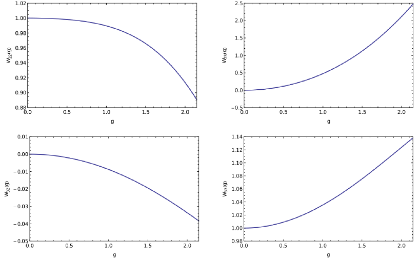
As a crosscheck of the robustness of our numerical approach we have computed explicitly the function $W(\mu)$ for $N_{\mathrm{\scriptstyle f}}=3$, using our numerical integration and $W=\mathbf{1}$ as an initial condition, set at an extremely small value of the coupling. Our result for $W$, displayed in Fig. 13, can then be fitted to an ansatz where $J$ is taken to have a polynomial dependence in $\kern 1.0pt\overline{\kern-1.0ptg\kern 0.0pt}\kern 1.0pt^{2}$, to check whether the first coefficient $J_{1}$ is compatible within systematic fit errors (obtained by trying different polynomial orders up to $\mathcal{O}(\kern 1.0pt\overline{\kern-1.0ptg\kern 0.0pt}\kern 1.0pt^{8})$ and coupling values for the initial condition) with the one quoted in Eq.(2.30) of [48]. Note that in order to have a direct comparison it has to be taken into account that we are using a different relative normalization between operators $O_{2}$, $O_{3}$ than the one in [48] which translates into a factor $-2$ and $-1/2$ respectively for $[J_{1}^{\rm fit}]_{23}$, $[J_{1}^{\rm fit}]_{32}$ and that, since we are working with the renormalization constants instead of the Wilson coefficients, the convention used for the $J$ is this work corresponds to $J^{T}$ in [48] . What we obtain is

$$J_{1}^{\rm fit}=\frac{1}{(4\pi)^{2}}\left(\begin{array}[]{cc}-1.0470(8)&70.13(38)\\ -1.39583(1)&5.78550(8)\end{array}\right)$$ (C.151)

which is indeed well-compatible with the above-mentioned result. Note that the coefficient $23$ contains a precise numerical value of the parameter $t$ employed in [48] to regularise the divergence of $J$ in $3-N_{\mathrm{\scriptstyle f}}$.

As a further crosscheck, we have also compared the result of computing the $N_{\mathrm{\scriptstyle f}}=2$ evolution with the two possible initial conditions. The outcome is that, if the value of the coupling at which $W=\mathbf{1}$ is sufficiently small, the two results are equal up to several significant figures down to values of the coupling $\kern 1.0pt\overline{\kern-1.0ptg\kern 0.0pt}\kern 1.0pt^{2}\gtrsim 2$, where the hadronic regimes is entered.

Figure 13: $W$ as a function of the coupling constant, with $N_{\mathrm{\scriptstyle f}}=3$ for operators $O_{2}$, $O_{3}$ fierz ”$+$”, in the ${\overline{\rm MS}}$ scheme.

D Finite parts of RI-MOM renormalisation constants in Landau gauge

In this appendix we gather the results for the finite part of the one-loop matching coefficients $[{\cal X}_{O}^{(1)}]_{\rm RI;lat}$ between the lattice and the RI-MOM scheme in Landau gauge. They can be extracted from [11] and are given by

$$[{\cal X}_{22}^{+,(1)}]_{\rm RI;lat} = 0.0272369\,c_{\rm sw}^{2}+0.0485167\,c_{\rm sw}-0.294894\,,$$

$$[{\cal X}_{23}^{+,(1)}]_{\rm RI;lat} = 0.0218485\,c_{\rm sw}^{2}+0.0632421\,c_{\rm sw}+0.0753979\,,$$

$$[{\cal X}_{32}^{+,(1)}]_{\rm RI;lat} = 0.00755569\,,$$

$$[{\cal X}_{33}^{+,(1)}]_{\rm RI;lat} = -0.00553581\,c_{\rm sw}^{2}-0.0463464\,c_{\rm sw}-0.362656\,,$$ (D.152)

$$[{\cal X}_{44}^{+,(1)}]_{\rm RI;lat} = 0.00538842\,c_{\rm sw}^{2}-0.0147254\,c_{\rm sw}-0.351294\,,$$

$$[{\cal X}_{45}^{+,(1)}]_{\rm RI;lat} = 0.000303451\,c_{\rm sw}^{2}+0.000878362\,c_{\rm sw}-0.00178318\,,$$

$$[{\cal X}_{54}^{+,(1)}]_{\rm RI;lat} = -0.0728282\,c_{\rm sw}^{2}-0.210807\,c_{\rm sw}-0.266293\,,$$

$$[{\cal X}_{55}^{+,(1)}]_{\rm RI;lat} = 0.0442301\,c_{\rm sw}^{2}+0.0977049\,c_{\rm sw}-0.290267\,.$$

$$[{\cal X}_{22}^{-,(1)}]_{\rm RI;lat} = 0.0272369\,c_{\rm sw}^{2}+0.0485167\,c_{\rm sw}-0.294894\,,$$

$$[{\cal X}_{23}^{-,(1)}]_{\rm RI;lat} = -0.0218485\,c_{\rm sw}^{2}-0.0632421\,c_{\rm sw}-0.0753979\,,$$

$$[{\cal X}_{32}^{-,(1)}]_{\rm RI;lat} = -0.00755569\,,$$

$$[{\cal X}_{33}^{-,(1)}]_{\rm RI;lat} = -0.00553581\,c_{\rm sw}^{2}-0.0463464\,c_{\rm sw}-0.362656\,,$$ (D.153)

$$[{\cal X}_{44}^{-,(1)}]_{\rm RI;lat} = -0.01646\,c_{\rm sw}^{2}-0.0779674\,c_{\rm sw}-0.374019\,,$$

$$[{\cal X}_{45}^{-,(1)}]_{\rm RI;lat} = -0.00151725\,c_{\rm sw}^{2}-0.00439181\,c_{\rm sw}+0.0013602\,,$$

$$[{\cal X}_{54}^{-,(1)}]_{\rm RI;lat} = 0.0145656\,c_{\rm sw}^{2}+0.0421614\,c_{\rm sw}+0.24599\,,$$

$$[{\cal X}_{55}^{-,(1)}]_{\rm RI;lat} = 0.0223817\,c_{\rm sw}^{2}+0.0344629\,c_{\rm sw}-0.257729\,.$$

E Finite parts of SF renormalisation constants

In this appendix we discuss how to determine the dependence on $a/L$ of the one-loop renormalization constants $Z^{(1)}$ defined in Section 3. The approach is essentially an application of the present context to the techniques discussed in Appendix D of [50].
Defining $\ell=L/a$ we will hence consider $F(\ell)=Z^{(1)}$ as a pure function of $\ell=\{\ell_{1},\dots,\ell_{N}\}$. We will also assume that all divergences have been removed from $F(\ell)$, which in general means linear divergences related to the additive renormalisation of quark masses and proportional to the one-loop value of the critical mass $m_{cr}^{(1)}$, and logarithmic divergences proportional to a LO anomalous dimension. To ensure the robustness of our method we performed separate fits, and we checked, for each ansatz, the fitted value of $\gamma^{(0)}$ was the correct one within the available precision. First of all a roundoff error has to be assigned to $F(\ell)$, which takes into account the uncertainties coming from the numerical computation itself. Following [50], we choose as an estimate for this error, in the case that the computation has been carried out in double precision,

$$\delta F(\ell)\equiv\epsilon(\ell)|F(\ell)|\,,$$ (E.154)

$$\epsilon(\ell)=\left(\frac{\ell}{2}\right)^{3}\times 10^{-14}.$$ (E.155)

As showed in Section 3 the expected behaviour of $F(\ell)$ leads to the consideration of an asymptotic expansion of the form

$$F(\ell)=\alpha_{0}+\sum_{k=1}^{n}\frac{1}{\ell^{k}}(\alpha_{k}+\beta_{k}\log\ell)+R_{n}(\ell)\,,$$ (E.156)

where the residue $R_{n}(\ell)$ is expected to decrease faster as $\ell\to\infty$ than any of the terms in the sum. To determine the coefficients $(\alpha_{k},\beta_{k})$ we minimise a quadratic form in the residues

$$\chi^{2}=(F-f\xi)^{T}(F-f\xi)\,,$$ (E.157)

where $F$ and $\xi$ are the $N-$ and $(2n+1)-$column vectors $(F(\ell_{1}),\dots,F(\ell))^{T}$ and
$(\alpha_{0},\alpha_{1},\dots,\alpha_{n},\beta_{1},\dots,\beta_{n})^{T}$, respectively, and $f$ is the $N\times(2n+1)$ matrix

$$f=\begin{pmatrix}1&\ell_{1}^{-1}&\cdots&\ell_{1}^{-n}&\ell_{1}^{-1}\log\ell_{1}&\cdots&\ell_{1}^{-n}\log\ell_{1}\\ 1&\ell_{2}^{-1}&\cdots&\ell_{2}^{-n}&\ell_{2}^{-1}\log\ell_{2}&\cdots&\ell_{2}^{-n}\log\ell_{2}\\ \vdots&\vdots&\vdots&\vdots&\vdots&\vdots&\vdots\\ 1&\ell_{N}^{-1}&\cdots&\ell_{N}^{-n}&\ell_{N}^{-1}\log\ell_{N}&\cdots&\ell_{N}^{-n}\log\ell_{N}\end{pmatrix}$$ (E.158)

Again following [50], we have not introduced a matrix of weights in the definition of $\chi^{2}$. A necessary condition to minimise $\chi^{2}$ is

$$f\xi=PF$$ (E.159)

where we have assumed that the columns of $f$ are linearly independent vectors (assuming $2n+1\ll N$), and $P$ is the projector onto the subspace of $\mathbb{R}^{N}$ generated by them. Eq. (E.159) can be solved using the singular value decomposition of $f$, which has the form of

$$f=USV^{T}$$ (E.160)

where $U$ is an $N\times(2n+1)$ matrix such that

$$U^{T}U=\mathbf{1}\quad,\quad UU^{T}=P$$ (E.161)

$S$ is diagonal, and $(2n+1)\times(2n+1)$ matrix $V$ is orthonormal. With this decomposition one has

$$\xi=VS^{-1}U^{T}F\,.$$ (E.162)

Finally, the uncertainty in the result for $\xi_{k}$ can be modelled using error propagation as

$$\delta\xi_{k}^{2}=\sum_{l=1}^{N}(VS^{-1}U^{T})_{kl}^{2}(\delta F)_{l}^{2}\,,$$ (E.163)

where $(\delta F)_{k}\equiv\delta F(\ell_{k})$.
As a remark on the above method regarding practical applications, it has to be pointed out that the choice of Eq. (E.157) for the quadratic form $\chi^{2}$ implies, in particular, that small values of $\ell$ might be given excessive weight. This problem has been dealt with by considering a range $[\ell_{min},\ell_{max}]$ with changing $\ell_{min}$. For this work the better convergence in results for $(\alpha_{k},\beta_{k})$ was given by $\ell_{min}=16$ and $\ell_{max}=46$. The estimation of systematic uncertainty of the fitting procedure has be performed using the proposal by the authors of [50]. We considered two independent fits at order $n$ and $n+1$, i.e. extending the Ansatz in Eq. (E.156) by terms $1/\ell^{n+1}$ and $\log\ell/\ell^{n+1}$ with coefficients $\alpha_{n+1}$ and $\beta_{n+1}$ respectively. The systematic uncertainty of the finite part $r_{0}=\alpha_{0}$ is defined as the difference of the value of the parameter $\alpha_{0}$ extracted by the two different fits. In the present work we have used $n=2$ in the fit Ansatz for the $\mathcal{O}$(a)-improved data, and $n=3$ for unimproved ones.

$\alpha$	$s$	$(r_{0})_{23}^{+}(c_{sw}=0)$	$(r_{0})_{23}^{-}(c_{sw}=0)$
0	$1$	$\begin{pmatrix}-0.2973(1)&0.12889(6)\\ 0.02613(1)&-0.20350(10)\end{pmatrix}$	$\begin{pmatrix}-0.3055(1)&0.008223(4)\\ -0.02778(1)&-0.19359(9)\end{pmatrix}$
	$2$	$\begin{pmatrix}-0.3027(1)&0.13105(6)\\ 0.02322(1)&-0.20234(9)\end{pmatrix}$	$\begin{pmatrix}-0.3212(2)&0.03063(1)\\ -0.03590(2)&-0.18199(8)\end{pmatrix}$
	$3$	$\begin{pmatrix}-0.3172(1)&0.13685(7)\\ 0.03615(2)&-0.20751(10)\end{pmatrix}$	$\begin{pmatrix}-0.3252(2)&0.03643(2)\\ -0.02962(1)&-0.19096(9)\end{pmatrix}$
	$4$	$\begin{pmatrix}-0.2991(1)&0.11812(6)\\ 0.03093(1)&-0.17471(8)\end{pmatrix}$	$\begin{pmatrix}-0.3104(1)&0.03794(2)\\ -0.03310(2)&-0.16164(8)\end{pmatrix}$
	$5$	$\begin{pmatrix}-0.3045(1)&0.12028(6)\\ 0.02802(1)&-0.17355(8)\end{pmatrix}$	$\begin{pmatrix}-0.3261(2)&0.06035(3)\\ -0.04123(2)&-0.15004(7)\end{pmatrix}$
	$6$	$\begin{pmatrix}-0.3190(2)&0.12608(6)\\ 0.04095(2)&-0.17872(8)\end{pmatrix}$	$\begin{pmatrix}-0.3302(2)&0.06615(3)\\ -0.03494(2)&-0.15901(7)\end{pmatrix}$
3/2	$1$	$\begin{pmatrix}-0.3100(1)&0.12889(6)\\ 0.02613(1)&-0.2161(1)\end{pmatrix}$	$\begin{pmatrix}-0.3181(2)&0.008223(4)\\ -0.02778(1)&-0.20623(10)\end{pmatrix}$
	$2$	$\begin{pmatrix}-0.3154(1)&0.13105(6)\\ 0.02322(1)&-0.2150(1)\end{pmatrix}$	$\begin{pmatrix}-0.3338(2)&0.03063(1)\\ -0.03590(2)&-0.19462(9)\end{pmatrix}$
	$3$	$\begin{pmatrix}-0.3299(2)&0.13685(7)\\ 0.03615(2)&-0.2201(1)\end{pmatrix}$	$\begin{pmatrix}-0.3379(2)&0.03643(2)\\ -0.02962(1)&-0.20360(9)\end{pmatrix}$
	$4$	$\begin{pmatrix}-0.3118(1)&0.11812(6)\\ 0.03093(1)&-0.18734(9)\end{pmatrix}$	$\begin{pmatrix}-0.3231(2)&0.03794(2)\\ -0.03310(2)&-0.17428(8)\end{pmatrix}$
	$5$	$\begin{pmatrix}-0.3172(1)&0.12028(6)\\ 0.02802(1)&-0.18618(9)\end{pmatrix}$	$\begin{pmatrix}-0.3387(2)&0.06035(3)\\ -0.04123(2)&-0.16267(8)\end{pmatrix}$
	$6$	$\begin{pmatrix}-0.3317(2)&0.12608(6)\\ 0.04095(2)&-0.19135(9)\end{pmatrix}$	$\begin{pmatrix}-0.3428(2)&0.06615(3)\\ -0.03494(2)&-0.17165(8)\end{pmatrix}$
1	$1$	$\begin{pmatrix}-0.3057(1)&0.12889(6)\\ 0.02613(1)&-0.21192(10)\end{pmatrix}$	$\begin{pmatrix}-0.3139(1)&0.008223(4)\\ -0.02778(1)&-0.20202(9)\end{pmatrix}$
	$2$	$\begin{pmatrix}-0.3111(1)&0.13105(6)\\ 0.02322(1)&-0.21076(10)\end{pmatrix}$	$\begin{pmatrix}-0.3296(2)&0.03063(1)\\ -0.03590(2)&-0.19041(9)\end{pmatrix}$
	$3$	$\begin{pmatrix}-0.3257(2)&0.13685(7)\\ 0.03615(2)&-0.2159(1)\end{pmatrix}$	$\begin{pmatrix}-0.3336(2)&0.03643(2)\\ -0.02962(1)&-0.19938(9)\end{pmatrix}$
	$4$	$\begin{pmatrix}-0.3075(1)&0.11812(6)\\ 0.03093(1)&-0.18313(9)\end{pmatrix}$	$\begin{pmatrix}-0.3188(2)&0.03794(2)\\ -0.03310(2)&-0.17007(8)\end{pmatrix}$
	$5$	$\begin{pmatrix}-0.3129(1)&0.12028(6)\\ 0.02802(1)&-0.18197(9)\end{pmatrix}$	$\begin{pmatrix}-0.3345(2)&0.06035(3)\\ -0.04123(2)&-0.15846(7)\end{pmatrix}$
	$6$	$\begin{pmatrix}-0.3275(2)&0.12608(6)\\ 0.04095(2)&-0.18714(9)\end{pmatrix}$	$\begin{pmatrix}-0.3386(2)&0.06615(3)\\ -0.03494(2)&-0.16744(8)\end{pmatrix}$

Table 3: Numerical results of the 1-loop finite parts for operators VA-AV,PS-SP in the $18$ SF renormalisation schemes under investigation defined by the source $s$ and the parameter $\alpha$ as in Eq. (3.99).

$\alpha$	$s$	$(r_{0})_{23}^{+}(c_{sw}=1)$	$(r_{0})_{23}^{-}(c_{sw}=1)$
0	$1$	$\begin{pmatrix}-0.22165(6)&0.21392(6)\\ 0.026133(6)&-0.25536(2)\end{pmatrix}$	$\begin{pmatrix}-0.22981(8)&-0.0767(1)\\ -0.027786(8)&-0.24544(3)\end{pmatrix}$
	$2$	$\begin{pmatrix}-0.22703(5)&0.21608(6)\\ 0.02324(1)&-0.25420(2)\end{pmatrix}$	$\begin{pmatrix}-0.24545(4)&-0.05439(7)\\ -0.035896(8)&-0.233856(10)\end{pmatrix}$
	$3$	$\begin{pmatrix}-0.24151(2)&0.22187(7)\\ 0.03613(2)&-0.25936(3)\end{pmatrix}$	$\begin{pmatrix}-0.24950(3)&-0.04859(6)\\ -0.029622(1)&-0.24282(2)\end{pmatrix}$
	$4$	$\begin{pmatrix}-0.22344(6)&0.20317(4)\\ 0.030919(6)&-0.22664(5)\end{pmatrix}$	$\begin{pmatrix}-0.23475(7)&-0.04710(4)\\ -0.033097(6)&-0.21357(5)\end{pmatrix}$
	$5$	$\begin{pmatrix}-0.22882(4)&0.20532(5)\\ 0.0280232(1)&-0.22548(5)\end{pmatrix}$	$\begin{pmatrix}-0.25039(3)&-0.02475(2)\\ -0.04121(2)&-0.20199(7)\end{pmatrix}$
	$6$	$\begin{pmatrix}-0.24330(1)&0.21111(6)\\ 0.04092(3)&-0.23064(4)\end{pmatrix}$	$\begin{pmatrix}-0.25444(2)&-0.01896(3)\\ -0.03493(1)&-0.21095(6)\end{pmatrix}$
3/2	$1$	$\begin{pmatrix}-0.23423(2)&0.21392(6)\\ 0.026133(6)&-0.26795(7)\end{pmatrix}$	$\begin{pmatrix}-0.24239(3)&-0.0767(1)\\ -0.027786(8)&-0.25803(8)\end{pmatrix}$
	$2$	$\begin{pmatrix}-0.239614(2)&0.21608(6)\\ 0.02324(1)&-0.26679(7)\end{pmatrix}$	$\begin{pmatrix}-0.258036(7)&-0.05439(7)\\ -0.035896(8)&-0.24644(6)\end{pmatrix}$
	$3$	$\begin{pmatrix}-0.25409(3)&0.22187(7)\\ 0.03613(2)&-0.27195(8)\end{pmatrix}$	$\begin{pmatrix}-0.26209(1)&-0.04859(6)\\ -0.029622(1)&-0.25541(7)\end{pmatrix}$
	$4$	$\begin{pmatrix}-0.23602(1)&0.20317(4)\\ 0.030919(6)&-0.239229(3)\end{pmatrix}$	$\begin{pmatrix}-0.24733(2)&-0.04710(4)\\ -0.033097(6)&-0.226161(3)\end{pmatrix}$
	$5$	$\begin{pmatrix}-0.241406(4)&0.20532(5)\\ 0.0280232(1)&-0.238070(6)\end{pmatrix}$	$\begin{pmatrix}-0.26298(2)&-0.02475(2)\\ -0.04121(2)&-0.21458(3)\end{pmatrix}$
	$6$	$\begin{pmatrix}-0.25589(3)&0.21111(6)\\ 0.04092(3)&-0.243229(6)\end{pmatrix}$	$\begin{pmatrix}-0.26703(3)&-0.01896(3)\\ -0.03493(1)&-0.22354(1)\end{pmatrix}$
1	$1$	$\begin{pmatrix}-0.23004(3)&0.21392(6)\\ 0.026133(6)&-0.26375(5)\end{pmatrix}$	$\begin{pmatrix}-0.23820(5)&-0.0767(1)\\ -0.027786(8)&-0.25383(6)\end{pmatrix}$
	$2$	$\begin{pmatrix}-0.23542(1)&0.21608(6)\\ 0.02324(1)&-0.26259(5)\end{pmatrix}$	$\begin{pmatrix}-0.253840(9)&-0.05439(7)\\ -0.035896(8)&-0.24225(4)\end{pmatrix}$
	$3$	$\begin{pmatrix}-0.24990(2)&0.22187(7)\\ 0.03613(2)&-0.26775(6)\end{pmatrix}$	$\begin{pmatrix}-0.2578952(9)&-0.04859(6)\\ -0.029622(1)&-0.25121(6)\end{pmatrix}$
	$4$	$\begin{pmatrix}-0.23183(3)&0.20317(4)\\ 0.030919(6)&-0.23503(2)\end{pmatrix}$	$\begin{pmatrix}-0.24314(4)&-0.04710(4)\\ -0.033097(6)&-0.22197(2)\end{pmatrix}$
	$5$	$\begin{pmatrix}-0.23721(1)&0.20532(5)\\ 0.0280232(1)&-0.23387(2)\end{pmatrix}$	$\begin{pmatrix}-0.258780(6)&-0.02475(2)\\ -0.04121(2)&-0.21038(4)\end{pmatrix}$
	$6$	$\begin{pmatrix}-0.25169(2)&0.21111(6)\\ 0.04092(3)&-0.23903(1)\end{pmatrix}$	$\begin{pmatrix}-0.26283(1)&-0.01896(3)\\ -0.03493(1)&-0.21934(3)\end{pmatrix}$

Table 4: Numerical results of the 1-loop finite parts for operators VA-AV,PS-SP in the $18$ SF renormalisation schemes under investigation defined by the source $s$ and the parameter $\alpha$ as in Eq. (3.99). These results have been computed including the clover term in the fermonic action.

$\alpha$	$s$	$(r_{0})_{45}^{+}(c_{sw}=0)$	$(r_{0})_{45}^{-}(c_{sw}=0)$
0	$1$	$\begin{pmatrix}-0.20786(10)&-0.008176(4)\\ -0.16835(8)&-0.3844(2)\end{pmatrix}$	$\begin{pmatrix}-0.18729(9)&0.012475(6)\\ 0.3886(2)&-0.2278(1)\end{pmatrix}$
	$2$	$\begin{pmatrix}-0.20612(10)&-0.008902(4)\\ -0.15539(8)&-0.3898(2)\end{pmatrix}$	$\begin{pmatrix}-0.19077(9)&0.010444(5)\\ 0.3826(2)&-0.2313(1)\end{pmatrix}$
	$3$	$\begin{pmatrix}-0.20882(10)&-0.007780(4)\\ -0.15920(8)&-0.3882(2)\end{pmatrix}$	$\begin{pmatrix}-0.18302(9)&0.014967(7)\\ 0.3788(2)&-0.2335(1)\end{pmatrix}$
	$4$	$\begin{pmatrix}-0.18240(8)&-0.009086(4)\\ -0.11374(6)&-0.3863(2)\end{pmatrix}$	$\begin{pmatrix}-0.15486(7)&0.014097(7)\\ 0.3496(2)&-0.2298(1)\end{pmatrix}$
	$5$	$\begin{pmatrix}-0.18066(8)&-0.009811(5)\\ -0.10078(5)&-0.3917(2)\end{pmatrix}$	$\begin{pmatrix}-0.15835(7)&0.012065(6)\\ 0.3436(2)&-0.2333(1)\end{pmatrix}$
	$6$	$\begin{pmatrix}-0.18335(9)&-0.008689(4)\\ -0.10459(5)&-0.3901(2)\end{pmatrix}$	$\begin{pmatrix}-0.15059(7)&0.016589(8)\\ 0.3398(2)&-0.2355(1)\end{pmatrix}$
3/2	$1$	$\begin{pmatrix}-0.2205(1)&-0.008176(4)\\ -0.16835(8)&-0.3970(2)\end{pmatrix}$	$\begin{pmatrix}-0.19992(9)&0.012475(6)\\ 0.3886(2)&-0.2404(1)\end{pmatrix}$
	$2$	$\begin{pmatrix}-0.2188(1)&-0.008902(4)\\ -0.15539(8)&-0.4024(2)\end{pmatrix}$	$\begin{pmatrix}-0.20341(10)&0.010444(5)\\ 0.3826(2)&-0.2439(1)\end{pmatrix}$
	$3$	$\begin{pmatrix}-0.2214(1)&-0.007780(4)\\ -0.15920(8)&-0.4008(2)\end{pmatrix}$	$\begin{pmatrix}-0.19565(9)&0.014967(7)\\ 0.3788(2)&-0.2462(1)\end{pmatrix}$
	$4$	$\begin{pmatrix}-0.19503(9)&-0.009086(4)\\ -0.11374(6)&-0.3989(2)\end{pmatrix}$	$\begin{pmatrix}-0.16750(8)&0.014097(7)\\ 0.3496(2)&-0.2424(1)\end{pmatrix}$
	$5$	$\begin{pmatrix}-0.19329(9)&-0.009811(5)\\ -0.10078(5)&-0.4043(2)\end{pmatrix}$	$\begin{pmatrix}-0.17098(8)&0.012065(6)\\ 0.3436(2)&-0.2459(1)\end{pmatrix}$
	$6$	$\begin{pmatrix}-0.19599(9)&-0.008689(4)\\ -0.10459(5)&-0.4028(2)\end{pmatrix}$	$\begin{pmatrix}-0.16322(8)&0.016589(8)\\ 0.3398(2)&-0.2481(1)\end{pmatrix}$
1	$1$	$\begin{pmatrix}-0.2163(1)&-0.008176(4)\\ -0.16835(8)&-0.3928(2)\end{pmatrix}$	$\begin{pmatrix}-0.19571(9)&0.012475(6)\\ 0.3886(2)&-0.2362(1)\end{pmatrix}$
	$2$	$\begin{pmatrix}-0.2145(1)&-0.008902(4)\\ -0.15539(8)&-0.3982(2)\end{pmatrix}$	$\begin{pmatrix}-0.19920(9)&0.010444(5)\\ 0.3826(2)&-0.2397(1)\end{pmatrix}$
	$3$	$\begin{pmatrix}-0.2172(1)&-0.007780(4)\\ -0.15920(8)&-0.3966(2)\end{pmatrix}$	$\begin{pmatrix}-0.19144(9)&0.014967(7)\\ 0.3788(2)&-0.2419(1)\end{pmatrix}$
	$4$	$\begin{pmatrix}-0.19082(9)&-0.009086(4)\\ -0.11374(6)&-0.3947(2)\end{pmatrix}$	$\begin{pmatrix}-0.16329(8)&0.014097(7)\\ 0.3496(2)&-0.2382(1)\end{pmatrix}$
	$5$	$\begin{pmatrix}-0.18908(9)&-0.009811(5)\\ -0.10078(5)&-0.4001(2)\end{pmatrix}$	$\begin{pmatrix}-0.16677(8)&0.012065(6)\\ 0.3436(2)&-0.2417(1)\end{pmatrix}$
	$6$	$\begin{pmatrix}-0.19177(9)&-0.008689(4)\\ -0.10459(5)&-0.3985(2)\end{pmatrix}$	$\begin{pmatrix}-0.15901(7)&0.016589(8)\\ 0.3398(2)&-0.2439(1)\end{pmatrix}$

Table 5: Numerical results of the 1-loop finite parts for operators PS+SP,T$\tilde{\text{T}}$ in the $18$ SF renormalisation schemes under investigation defined by the source $s$ and the parameter $\alpha$ as in Eq. (3.99).

$\alpha$	$s$	$(r_{0})_{45}^{+}(c_{sw}=1)$	$(r_{0})_{45}^{-}(c_{sw}=1)$
0	$1$	$\begin{pmatrix}-0.21719(1)&-0.0069948(4)\\ -0.4517(3)&-0.24249(6)\end{pmatrix}$	$\begin{pmatrix}-0.28168(3)&0.006568(2)\\ 0.4451(2)&-0.17105(8)\end{pmatrix}$
	$2$	$\begin{pmatrix}-0.215453(7)&-0.007719(1)\\ -0.4388(2)&-0.24787(4)\end{pmatrix}$	$\begin{pmatrix}-0.28516(4)&0.004541(6)\\ 0.4392(2)&-0.17453(6)\end{pmatrix}$
	$3$	$\begin{pmatrix}-0.21814(1)&-0.0065985(6)\\ -0.4426(2)&-0.24629(4)\end{pmatrix}$	$\begin{pmatrix}-0.27742(2)&0.009054(4)\\ 0.4354(2)&-0.17674(6)\end{pmatrix}$
	$4$	$\begin{pmatrix}-0.19179(6)&-0.007902(2)\\ -0.3972(1)&-0.24444(5)\end{pmatrix}$	$\begin{pmatrix}-0.24934(5)&0.008185(2)\\ 0.4062(1)&-0.17299(7)\end{pmatrix}$
	$5$	$\begin{pmatrix}-0.19006(6)&-0.008626(4)\\ -0.38433(7)&-0.24982(3)\end{pmatrix}$	$\begin{pmatrix}-0.25281(4)&0.006158(2)\\ 0.40026(9)&-0.17647(6)\end{pmatrix}$
	$6$	$\begin{pmatrix}-0.19275(6)&-0.007506(2)\\ -0.38813(7)&-0.24823(3)\end{pmatrix}$	$\begin{pmatrix}-0.24507(6)&0.010672(8)\\ 0.39646(9)&-0.17869(6)\end{pmatrix}$
3/2	$1$	$\begin{pmatrix}-0.22978(6)&-0.0069948(4)\\ -0.4517(3)&-0.255079(8)\end{pmatrix}$	$\begin{pmatrix}-0.29427(8)&0.006568(2)\\ 0.4451(2)&-0.18363(3)\end{pmatrix}$
	$2$	$\begin{pmatrix}-0.22804(6)&-0.007719(1)\\ -0.4388(2)&-0.260460(9)\end{pmatrix}$	$\begin{pmatrix}-0.29775(9)&0.004541(6)\\ 0.4392(2)&-0.18711(1)\end{pmatrix}$
	$3$	$\begin{pmatrix}-0.23073(6)&-0.0065985(6)\\ -0.4426(2)&-0.258875(8)\end{pmatrix}$	$\begin{pmatrix}-0.29001(7)&0.009054(4)\\ 0.4354(2)&-0.18933(1)\end{pmatrix}$
	$4$	$\begin{pmatrix}-0.204380(9)&-0.007902(2)\\ -0.3972(1)&-0.257024(3)\end{pmatrix}$	$\begin{pmatrix}-0.2619224(2)&0.008185(2)\\ 0.4062(1)&-0.18558(3)\end{pmatrix}$
	$5$	$\begin{pmatrix}-0.20264(1)&-0.008626(4)\\ -0.38433(7)&-0.26241(1)\end{pmatrix}$	$\begin{pmatrix}-0.265398(7)&0.006158(2)\\ 0.40026(9)&-0.189057(9)\end{pmatrix}$
	$6$	$\begin{pmatrix}-0.205331(9)&-0.007506(2)\\ -0.38813(7)&-0.26082(1)\end{pmatrix}$	$\begin{pmatrix}-0.257660(10)&0.010672(8)\\ 0.39646(9)&-0.191276(8)\end{pmatrix}$
1	$1$	$\begin{pmatrix}-0.22558(4)&-0.0069948(4)\\ -0.4517(3)&-0.25088(2)\end{pmatrix}$	$\begin{pmatrix}-0.29007(7)&0.006568(2)\\ 0.4451(2)&-0.17944(5)\end{pmatrix}$
	$2$	$\begin{pmatrix}-0.22384(4)&-0.007719(1)\\ -0.4388(2)&-0.256264(6)\end{pmatrix}$	$\begin{pmatrix}-0.29355(7)&0.004541(6)\\ 0.4392(2)&-0.18292(3)\end{pmatrix}$
	$3$	$\begin{pmatrix}-0.22653(4)&-0.0065985(6)\\ -0.4426(2)&-0.254679(7)\end{pmatrix}$	$\begin{pmatrix}-0.28581(6)&0.009054(4)\\ 0.4354(2)&-0.18514(3)\end{pmatrix}$
	$4$	$\begin{pmatrix}-0.20018(2)&-0.007902(2)\\ -0.3972(1)&-0.25283(2)\end{pmatrix}$	$\begin{pmatrix}-0.25773(2)&0.008185(2)\\ 0.4062(1)&-0.18138(4)\end{pmatrix}$
	$5$	$\begin{pmatrix}-0.19845(3)&-0.008626(4)\\ -0.38433(7)&-0.258210(1)\end{pmatrix}$	$\begin{pmatrix}-0.261202(9)&0.006158(2)\\ 0.40026(9)&-0.18486(2)\end{pmatrix}$
	$6$	$\begin{pmatrix}-0.20114(2)&-0.007506(2)\\ -0.38813(7)&-0.256624(2)\end{pmatrix}$	$\begin{pmatrix}-0.25346(3)&0.010672(8)\\ 0.39646(9)&-0.18708(2)\end{pmatrix}$

Table 6: Numerical results of the 1-loop finite parts for operators PS+SP,T$\tilde{\text{T}}$ in the $18$ SF renormalisation schemes under investigation defined by the source $s$ and the parameter $\alpha$ as in Eq. (3.99). These results have been computed including the clover term in the fermonic action.

F NLO anomalous dimension matrices in SF schemes

$\alpha$	$s$	${\gamma^{(1)}}_{23}^{+}$
0	$1$	$\begin{pmatrix}0.001519(10)+N_{f}[-0.000057850(2)]&0.00983(2)+N_{f}[-0.00034710(1)]\\ 0.006188(1)+N_{f}[-0.000080203]&-0.006776(8)+N_{f}[-0.00001842(2)]\end{pmatrix}$
	$2$	$\begin{pmatrix}0.001080(8)+N_{f}[-0.000057850(2)]&0.00936(2)+N_{f}[-0.00034710(1)]\\ 0.005504(3)+N_{f}[-0.000080203]&-0.006855(7)+N_{f}[-0.00001842(2)]\end{pmatrix}$
	$3$	$\begin{pmatrix}-0.001673(4)+N_{f}[-0.000057850(2)]&0.00870(2)+N_{f}[-0.00034710(1)]\\ 0.008552(4)+N_{f}[-0.000080203]&-0.00651(1)+N_{f}[-0.00001842(2)]\end{pmatrix}$
	$4$	$\begin{pmatrix}0.000936(10)+N_{f}[-0.000057850(2)]&0.00743(2)+N_{f}[-0.00034710(1)]\\ 0.007320(1)+N_{f}[-0.000080203]&-0.00290(2)+N_{f}[-0.00001842(2)]\end{pmatrix}$
	$5$	$\begin{pmatrix}0.000497(6)+N_{f}[-0.000057850(2)]&0.00695(2)+N_{f}[-0.00034710(1)]\\ 0.0066351(1)+N_{f}[-0.000080203]&-0.00297(2)+N_{f}[-0.00001842(2)]\end{pmatrix}$
	$6$	$\begin{pmatrix}-0.002256(4)+N_{f}[-0.000057850(2)]&0.00629(2)+N_{f}[-0.00034710(1)]\\ 0.009684(7)+N_{f}[-0.000080203]&-0.00263(2)+N_{f}[-0.00001842(2)]\end{pmatrix}$
3/2	$1$	$\begin{pmatrix}-0.000022(3)+N_{f}[-0.000057850(2)]&0.00983(2)+N_{f}[-0.00034710(1)]\\ 0.006188(1)+N_{f}[-0.000080203]&-0.00832(2)+N_{f}[-0.00001842(2)]\end{pmatrix}$
	$2$	$\begin{pmatrix}-0.000461(1)+N_{f}[-0.000057850(2)]&0.00936(2)+N_{f}[-0.00034710(1)]\\ 0.005504(3)+N_{f}[-0.000080203]&-0.00840(2)+N_{f}[-0.00001842(2)]\end{pmatrix}$
	$3$	$\begin{pmatrix}-0.003214(6)+N_{f}[-0.000057850(2)]&0.00870(3)+N_{f}[-0.00034710(1)]\\ 0.008552(4)+N_{f}[-0.000080203]&-0.00805(3)+N_{f}[-0.00001842(2)]\end{pmatrix}$
	$4$	$\begin{pmatrix}-0.000605(3)+N_{f}[-0.000057850(2)]&0.00743(1)+N_{f}[-0.00034710(1)]\\ 0.007320(1)+N_{f}[-0.000080203]&-0.004438(2)+N_{f}[-0.00001842(2)]\end{pmatrix}$
	$5$	$\begin{pmatrix}-0.0010440(6)+N_{f}[-0.000057850(2)]&0.00695(1)+N_{f}[-0.00034710(1)]\\ 0.0066351(1)+N_{f}[-0.000080203]&-0.004516(2)+N_{f}[-0.00001842(2)]\end{pmatrix}$
	$6$	$\begin{pmatrix}-0.003797(7)+N_{f}[-0.000057850(2)]&0.00629(2)+N_{f}[-0.00034710(1)]\\ 0.009684(7)+N_{f}[-0.000080203]&-0.004167(4)+N_{f}[-0.00001842(2)]\end{pmatrix}$
1	$1$	$\begin{pmatrix}0.000492(5)+N_{f}[-0.000057850(2)]&0.00983(2)+N_{f}[-0.00034710(1)]\\ 0.006188(1)+N_{f}[-0.000080203]&-0.00780(2)+N_{f}[-0.00001842(2)]\end{pmatrix}$
	$2$	$\begin{pmatrix}0.000053(3)+N_{f}[-0.000057850(2)]&0.00936(2)+N_{f}[-0.00034710(1)]\\ 0.005504(3)+N_{f}[-0.000080203]&-0.00788(2)+N_{f}[-0.00001842(2)]\end{pmatrix}$
	$3$	$\begin{pmatrix}-0.002700(4)+N_{f}[-0.000057850(2)]&0.00870(2)+N_{f}[-0.00034710(1)]\\ 0.008552(4)+N_{f}[-0.000080203]&-0.00753(2)+N_{f}[-0.00001842(2)]\end{pmatrix}$
	$4$	$\begin{pmatrix}-0.000092(5)+N_{f}[-0.000057850(2)]&0.00743(1)+N_{f}[-0.00034710(1)]\\ 0.007320(1)+N_{f}[-0.000080203]&-0.003924(7)+N_{f}[-0.00001842(2)]\end{pmatrix}$
	$5$	$\begin{pmatrix}-0.000530(2)+N_{f}[-0.000057850(2)]&0.00695(1)+N_{f}[-0.00034710(1)]\\ 0.0066351(1)+N_{f}[-0.000080203]&-0.004002(7)+N_{f}[-0.00001842(2)]\end{pmatrix}$
	$6$	$\begin{pmatrix}-0.003283(5)+N_{f}[-0.000057850(2)]&0.00629(2)+N_{f}[-0.00034710(1)]\\ 0.009684(7)+N_{f}[-0.000080203]&-0.003654(6)+N_{f}[-0.00001842(2)]\end{pmatrix}$

$\alpha$	$s$	${\gamma^{(1)}}_{23}^{-}$
0	$1$	$\begin{pmatrix}0.00051(1)+N_{f}[-0.000118203(2)]&-0.00803(4)+N_{f}[0.00070922(1)]\\ -0.006546(2)+N_{f}[0.000063796]&-0.00660(1)+N_{f}[0.00056285(2)]\end{pmatrix}$
	$2$	$\begin{pmatrix}-0.002017(7)+N_{f}[-0.000118203(2)]&-0.00577(2)+N_{f}[0.00070922(1)]\\ -0.008464(2)+N_{f}[0.000063796]&-0.004564(4)+N_{f}[0.00056285(2)]\end{pmatrix}$
	$3$	$\begin{pmatrix}-0.002036(5)+N_{f}[-0.000118203(2)]&-0.00609(2)+N_{f}[0.00070922(1)]\\ -0.0069803(3)+N_{f}[0.000063796]&-0.006138(8)+N_{f}[0.00056285(2)]\end{pmatrix}$
	$4$	$\begin{pmatrix}-0.00049(1)+N_{f}[-0.000118203(2)]&-0.00498(2)+N_{f}[0.00070922(1)]\\ -0.007802(1)+N_{f}[0.000063796]&-0.00229(2)+N_{f}[0.00056285(2)]\end{pmatrix}$
	$5$	$\begin{pmatrix}-0.003025(6)+N_{f}[-0.000118203(2)]&-0.00272(1)+N_{f}[0.00070922(1)]\\ -0.009719(5)+N_{f}[0.000063796]&-0.00026(3)+N_{f}[0.00056285(2)]\end{pmatrix}$
	$6$	$\begin{pmatrix}-0.003045(4)+N_{f}[-0.000118203(2)]&-0.00305(1)+N_{f}[0.00070922(1)]\\ -0.008236(3)+N_{f}[0.000063796]&-0.00183(2)+N_{f}[0.00056285(2)]\end{pmatrix}$
3/2	$1$	$\begin{pmatrix}-0.001026(6)+N_{f}[-0.000118203(2)]&-0.00803(4)+N_{f}[0.00070922(1)]\\ -0.006546(2)+N_{f}[0.000063796]&-0.00814(3)+N_{f}[0.00056285(2)]\end{pmatrix}$
	$2$	$\begin{pmatrix}-0.003558(2)+N_{f}[-0.000118203(2)]&-0.00577(2)+N_{f}[0.00070922(1)]\\ -0.008464(2)+N_{f}[0.000063796]&-0.00611(2)+N_{f}[0.00056285(2)]\end{pmatrix}$
	$3$	$\begin{pmatrix}-0.003577(2)+N_{f}[-0.000118203(2)]&-0.00609(2)+N_{f}[0.00070922(1)]\\ -0.0069803(3)+N_{f}[0.000063796]&-0.00768(2)+N_{f}[0.00056285(2)]\end{pmatrix}$
	$4$	$\begin{pmatrix}-0.002034(3)+N_{f}[-0.000118203(2)]&-0.00498(1)+N_{f}[0.00070922(1)]\\ -0.007802(1)+N_{f}[0.000063796]&-0.003835(2)+N_{f}[0.00056285(2)]\end{pmatrix}$
	$5$	$\begin{pmatrix}-0.004566(5)+N_{f}[-0.000118203(2)]&-0.002722(8)+N_{f}[0.00070922(1)]\\ -0.009719(5)+N_{f}[0.000063796]&-0.00180(1)+N_{f}[0.00056285(2)]\end{pmatrix}$
	$6$	$\begin{pmatrix}-0.004586(5)+N_{f}[-0.000118203(2)]&-0.00305(1)+N_{f}[0.00070922(1)]\\ -0.008236(3)+N_{f}[0.000063796]&-0.003374(6)+N_{f}[0.00056285(2)]\end{pmatrix}$
1	$1$	$\begin{pmatrix}-0.000512(8)+N_{f}[-0.000118203(2)]&-0.00803(4)+N_{f}[0.00070922(1)]\\ -0.006546(2)+N_{f}[0.000063796]&-0.00763(2)+N_{f}[0.00056285(2)]\end{pmatrix}$
	$2$	$\begin{pmatrix}-0.003044(2)+N_{f}[-0.000118203(2)]&-0.00577(2)+N_{f}[0.00070922(1)]\\ -0.008464(2)+N_{f}[0.000063796]&-0.00559(1)+N_{f}[0.00056285(2)]\end{pmatrix}$
	$3$	$\begin{pmatrix}-0.0030635(3)+N_{f}[-0.000118203(2)]&-0.00609(2)+N_{f}[0.00070922(1)]\\ -0.0069803(3)+N_{f}[0.000063796]&-0.00717(2)+N_{f}[0.00056285(2)]\end{pmatrix}$
	$4$	$\begin{pmatrix}-0.001521(6)+N_{f}[-0.000118203(2)]&-0.00498(1)+N_{f}[0.00070922(1)]\\ -0.007802(1)+N_{f}[0.000063796]&-0.003321(7)+N_{f}[0.00056285(2)]\end{pmatrix}$
	$5$	$\begin{pmatrix}-0.004052(3)+N_{f}[-0.000118203(2)]&-0.002722(8)+N_{f}[0.00070922(1)]\\ -0.009719(5)+N_{f}[0.000063796]&-0.00129(2)+N_{f}[0.00056285(2)]\end{pmatrix}$
	$6$	$\begin{pmatrix}-0.004072(3)+N_{f}[-0.000118203(2)]&-0.00305(1)+N_{f}[0.00070922(1)]\\ -0.008236(3)+N_{f}[0.000063796]&-0.00286(1)+N_{f}[0.00056285(2)]\end{pmatrix}$

$\alpha$	$s$	${\gamma^{(1)}}_{45}^{+}$
0	$1$	$\begin{pmatrix}0.002303(3)+N_{f}[0.00012884(1)]&-0.00169802(7)+N_{f}[0.0000026054(2)]\\ 0.00172(8)+N_{f}[0.00179861(4)]&0.00081(2)+N_{f}[-0.00035752(1)]\end{pmatrix}$
	$2$	$\begin{pmatrix}0.002685(2)+N_{f}[0.00012884(1)]&-0.0018770(3)+N_{f}[0.0000026054(2)]\\ 0.00336(7)+N_{f}[0.00179861(4)]&-0.00001(1)+N_{f}[-0.00035752(1)]\end{pmatrix}$
	$3$	$\begin{pmatrix}0.002077(4)+N_{f}[0.00012884(1)]&-0.0015930(3)+N_{f}[0.0000026054(2)]\\ 0.00232(7)+N_{f}[0.00179861(4)]&0.00046(1)+N_{f}[-0.00035752(1)]\end{pmatrix}$
	$4$	$\begin{pmatrix}0.00558(2)+N_{f}[0.00012884(1)]&-0.0019027(6)+N_{f}[0.0000026054(2)]\\ 0.00795(6)+N_{f}[0.00179861(4)]&0.00040(1)+N_{f}[-0.00035752(1)]\end{pmatrix}$
	$5$	$\begin{pmatrix}0.00597(2)+N_{f}[0.00012884(1)]&-0.002082(1)+N_{f}[0.0000026054(2)]\\ 0.00959(4)+N_{f}[0.00179861(4)]&-0.00043(1)+N_{f}[-0.00035752(1)]\end{pmatrix}$
	$6$	$\begin{pmatrix}0.00536(1)+N_{f}[0.00012884(1)]&-0.0017978(6)+N_{f}[0.0000026054(2)]\\ 0.00856(4)+N_{f}[0.00179861(4)]&0.000048(10)+N_{f}[-0.00035752(1)]\end{pmatrix}$
3/2	$1$	$\begin{pmatrix}0.00076(2)+N_{f}[0.00012884(1)]&-0.00169802(7)+N_{f}[0.0000026054(2)]\\ 0.00172(8)+N_{f}[0.00179861(4)]&-0.000727(3)+N_{f}[-0.00035752(1)]\end{pmatrix}$
	$2$	$\begin{pmatrix}0.00114(1)+N_{f}[0.00012884(1)]&-0.0018770(3)+N_{f}[0.0000026054(2)]\\ 0.00336(7)+N_{f}[0.00179861(4)]&-0.001556(3)+N_{f}[-0.00035752(1)]\end{pmatrix}$
	$3$	$\begin{pmatrix}0.00054(2)+N_{f}[0.00012884(1)]&-0.0015930(3)+N_{f}[0.0000026054(2)]\\ 0.00232(7)+N_{f}[0.00179861(4)]&-0.001082(3)+N_{f}[-0.00035752(1)]\end{pmatrix}$
	$4$	$\begin{pmatrix}0.004044(3)+N_{f}[0.00012884(1)]&-0.0019027(5)+N_{f}[0.0000026054(2)]\\ 0.00795(3)+N_{f}[0.00179861(4)]&-0.001138(2)+N_{f}[-0.00035752(1)]\end{pmatrix}$
	$5$	$\begin{pmatrix}0.004426(5)+N_{f}[0.00012884(1)]&-0.002082(1)+N_{f}[0.0000026054(2)]\\ 0.00959(2)+N_{f}[0.00179861(4)]&-0.001966(5)+N_{f}[-0.00035752(1)]\end{pmatrix}$
	$6$	$\begin{pmatrix}0.003817(3)+N_{f}[0.00012884(1)]&-0.0017978(5)+N_{f}[0.0000026054(2)]\\ 0.00856(2)+N_{f}[0.00179861(4)]&-0.001492(5)+N_{f}[-0.00035752(1)]\end{pmatrix}$
1	$1$	$\begin{pmatrix}0.00128(1)+N_{f}[0.00012884(1)]&-0.00169802(7)+N_{f}[0.0000026054(2)]\\ 0.00172(8)+N_{f}[0.00179861(4)]&-0.000214(7)+N_{f}[-0.00035752(1)]\end{pmatrix}$
	$2$	$\begin{pmatrix}0.00166(1)+N_{f}[0.00012884(1)]&-0.0018770(3)+N_{f}[0.0000026054(2)]\\ 0.00336(7)+N_{f}[0.00179861(4)]&-0.001042(3)+N_{f}[-0.00035752(1)]\end{pmatrix}$
	$3$	$\begin{pmatrix}0.00105(1)+N_{f}[0.00012884(1)]&-0.0015930(3)+N_{f}[0.0000026054(2)]\\ 0.00232(7)+N_{f}[0.00179861(4)]&-0.000568(3)+N_{f}[-0.00035752(1)]\end{pmatrix}$
	$4$	$\begin{pmatrix}0.004557(7)+N_{f}[0.00012884(1)]&-0.0019027(6)+N_{f}[0.0000026054(2)]\\ 0.00795(4)+N_{f}[0.00179861(4)]&-0.000624(6)+N_{f}[-0.00035752(1)]\end{pmatrix}$
	$5$	$\begin{pmatrix}0.004940(9)+N_{f}[0.00012884(1)]&-0.002082(1)+N_{f}[0.0000026054(2)]\\ 0.00959(3)+N_{f}[0.00179861(4)]&-0.001453(2)+N_{f}[-0.00035752(1)]\end{pmatrix}$
	$6$	$\begin{pmatrix}0.004331(7)+N_{f}[0.00012884(1)]&-0.0017978(5)+N_{f}[0.0000026054(2)]\\ 0.00856(2)+N_{f}[0.00179861(4)]&-0.000979(1)+N_{f}[-0.00035752(1)]\end{pmatrix}$

$\alpha$	$s$	${\gamma^{(1)}}_{45}^{-}$
0	$1$	$\begin{pmatrix}-0.01620(2)+N_{f}[0.00069509(2)]&0.001678(1)+N_{f}[-0.0000064430(8)]\\ 0.00879(7)+N_{f}[-0.002125401(8)]&0.00907(1)+N_{f}[-0.0004158697(7)]\end{pmatrix}$
	$2$	$\begin{pmatrix}-0.01676(2)+N_{f}[0.00069509(2)]&0.001156(2)+N_{f}[-0.0000064430(8)]\\ 0.00887(6)+N_{f}[-0.002125401(8)]&0.008779(9)+N_{f}[-0.0004158697(7)]\end{pmatrix}$
	$3$	$\begin{pmatrix}-0.01560(1)+N_{f}[0.00069509(2)]&0.002266(2)+N_{f}[-0.0000064430(8)]\\ 0.00841(6)+N_{f}[-0.002125401(8)]&0.008299(9)+N_{f}[-0.0004158697(7)]\end{pmatrix}$
	$4$	$\begin{pmatrix}-0.01236(2)+N_{f}[0.00069509(2)]&0.001914(1)+N_{f}[-0.0000064430(8)]\\ 0.00755(4)+N_{f}[-0.002125401(8)]&0.00896(1)+N_{f}[-0.0004158697(7)]\end{pmatrix}$
	$5$	$\begin{pmatrix}-0.01292(2)+N_{f}[0.00069509(2)]&0.0013917(10)+N_{f}[-0.0000064430(8)]\\ 0.00762(3)+N_{f}[-0.002125401(8)]&0.008664(8)+N_{f}[-0.0004158697(7)]\end{pmatrix}$
	$6$	$\begin{pmatrix}-0.01176(2)+N_{f}[0.00069509(2)]&0.002502(3)+N_{f}[-0.0000064430(8)]\\ 0.00716(3)+N_{f}[-0.002125401(8)]&0.008184(8)+N_{f}[-0.0004158697(7)]\end{pmatrix}$
3/2	$1$	$\begin{pmatrix}-0.01774(3)+N_{f}[0.00069509(2)]&0.001678(1)+N_{f}[-0.0000064430(8)]\\ 0.00879(7)+N_{f}[-0.002125401(8)]&0.007530(5)+N_{f}[-0.0004158697(7)]\end{pmatrix}$
	$2$	$\begin{pmatrix}-0.01830(4)+N_{f}[0.00069509(2)]&0.001156(2)+N_{f}[-0.0000064430(8)]\\ 0.00887(6)+N_{f}[-0.002125401(8)]&0.007238(3)+N_{f}[-0.0004158697(7)]\end{pmatrix}$
	$3$	$\begin{pmatrix}-0.01714(3)+N_{f}[0.00069509(2)]&0.002266(2)+N_{f}[-0.0000064430(8)]\\ 0.00841(6)+N_{f}[-0.002125401(8)]&0.006758(3)+N_{f}[-0.0004158697(7)]\end{pmatrix}$
	$4$	$\begin{pmatrix}-0.013901(2)+N_{f}[0.00069509(2)]&0.0019137(8)+N_{f}[-0.0000064430(8)]\\ 0.00755(3)+N_{f}[-0.002125401(8)]&0.007415(4)+N_{f}[-0.0004158697(7)]\end{pmatrix}$
	$5$	$\begin{pmatrix}-0.014461(4)+N_{f}[0.00069509(2)]&0.0013917(6)+N_{f}[-0.0000064430(8)]\\ 0.00762(2)+N_{f}[-0.002125401(8)]&0.007123(2)+N_{f}[-0.0004158697(7)]\end{pmatrix}$
	$6$	$\begin{pmatrix}-0.013305(5)+N_{f}[0.00069509(2)]&0.002502(2)+N_{f}[-0.0000064430(8)]\\ 0.00716(2)+N_{f}[-0.002125401(8)]&0.006643(2)+N_{f}[-0.0004158697(7)]\end{pmatrix}$
1	$1$	$\begin{pmatrix}-0.01722(3)+N_{f}[0.00069509(2)]&0.001678(1)+N_{f}[-0.0000064430(8)]\\ 0.00879(7)+N_{f}[-0.002125401(8)]&0.008043(7)+N_{f}[-0.0004158697(7)]\end{pmatrix}$
	$2$	$\begin{pmatrix}-0.01778(3)+N_{f}[0.00069509(2)]&0.001156(2)+N_{f}[-0.0000064430(8)]\\ 0.00887(6)+N_{f}[-0.002125401(8)]&0.007751(5)+N_{f}[-0.0004158697(7)]\end{pmatrix}$
	$3$	$\begin{pmatrix}-0.01663(2)+N_{f}[0.00069509(2)]&0.002266(2)+N_{f}[-0.0000064430(8)]\\ 0.00841(6)+N_{f}[-0.002125401(8)]&0.007271(5)+N_{f}[-0.0004158697(7)]\end{pmatrix}$
	$4$	$\begin{pmatrix}-0.013388(7)+N_{f}[0.00069509(2)]&0.0019137(10)+N_{f}[-0.0000064430(8)]\\ 0.00755(3)+N_{f}[-0.002125401(8)]&0.007928(6)+N_{f}[-0.0004158697(7)]\end{pmatrix}$
	$5$	$\begin{pmatrix}-0.013947(4)+N_{f}[0.00069509(2)]&0.0013917(6)+N_{f}[-0.0000064430(8)]\\ 0.00762(3)+N_{f}[-0.002125401(8)]&0.007637(4)+N_{f}[-0.0004158697(7)]\end{pmatrix}$
	$6$	$\begin{pmatrix}-0.01279(1)+N_{f}[0.00069509(2)]&0.002502(2)+N_{f}[-0.0000064430(8)]\\ 0.00716(3)+N_{f}[-0.002125401(8)]&0.007156(4)+N_{f}[-0.0004158697(7)]\end{pmatrix}$

References

- [1] A. Donini, V. Giménez, G. Martinelli, M. Talevi, and A. Vladikas, Nonperturbative renormalization of lattice four fermion operators without power subtractions, Eur. Phys. J. C10 (1999) 121–142, [hep-lat/9902030].
- [2] Alpha Collaboration, R. Frezzotti, P. A. Grassi, S. Sint, and P. Weisz, Lattice QCD with a chirally twisted mass term, JHEP 08 (2001) 058, [hep-lat/0101001].
- [3] C. Pena, S. Sint, and A. Vladikas, Twisted mass QCD and lattice approaches to the , JHEP 09 (2004) 069, [hep-lat/0405028].
- [4] R. Frezzotti and G. C. Rossi, Chirally improving Wilson fermions. II. Four-quark operators, JHEP 10 (2004) 070, [hep-lat/0407002].
- [5] M. Ciuchini, E. Franco, V. Lubicz, G. Martinelli, I. Scimemi, and L. Silvestrini, Next-to-leading order QCD corrections to effective Hamiltonians, Nucl. Phys. B523 (1998) 501–525, [hep-ph/9711402].
- [6] J. A. Bagger, K. T. Matchev, and R.-J. Zhang, QCD corrections to flavor changing neutral currents in the supersymmetric standard model, Phys. Lett. B412 (1997) 77–85, [hep-ph/9707225].
- [7] S. Narison and R. Tarrach, Higher Dimensional Renormalization Group Invariant Vacuum Condensates in Quantum Chromodynamics, Phys. Lett. B125 (1983) 217–222.
- [8] A. J. Buras, M. Misiak, and J. Urban, Two loop QCD anomalous dimensions of flavor changing four quark operators within and beyond the standard model, Nucl. Phys. B586 (2000) 397–426, [hep-ph/0005183].
- [9] A. J. Buras, M. Jamin, M. E. Lautenbacher, and P. H. Weisz, Effective Hamiltonians for and nonleptonic decays beyond the leading logarithmic approximation, Nucl. Phys. B370 (1992) 69–104. [Addendum: Nucl. Phys.B375,501(1992)].
- [10] A. J. Buras, M. Jamin, M. E. Lautenbacher, and P. H. Weisz, Two loop anomalous dimension matrix for weak nonleptonic decays I: , Nucl. Phys. B400 (1993) 37–74, [hep-ph/9211304].
- [11] M. Constantinou, P. Dimopoulos, R. Frezzotti, V. Lubicz, H. Panagopoulos, A. Skouroupathis, and F. Stylianou, Perturbative renormalization factors and corrections for lattice 4-fermion operators with improved fermion/gluon actions, Phys. Rev. D83 (2011) 074503, [arXiv:1011.6059].
- [12] R. Gupta, T. Bhattacharya, and S. R. Sharpe, Matrix elements of four fermion operators with quenched Wilson fermions, Phys. Rev. D55 (1997) 4036–4054, [hep-lat/9611023].
- [13] SWME Collaboration, J. Kim, W. Lee, J. Leem, S. R. Sharpe, and B. Yoon, Toolkit for staggered matrix elements, Phys. Rev. D90 (2014), no. 1 014504, [arXiv:1404.2368].
- [14] S. Capitani, M. Göckeler, R. Horsley, H. Perlt, P. E. L. Rakow, G. Schierholz, and A. Schiller, Renormalization and off-shell improvement in lattice perturbation theory, Nucl. Phys. B593 (2001) 183–228, [hep-lat/0007004].
- [15] S. Sint and R. Sommer, The Running coupling from the QCD Schrodinger functional: A One loop analysis, Nucl. Phys. B465 (1996) 71–98, [hep-lat/9508012].
- [16] M. Lüscher, R. Narayanan, P. Weisz, and U. Wolff, The Schrödinger functional: A Renormalizable probe for nonAbelian gauge theories, Nucl. Phys. B384 (1992) 168–228, [hep-lat/9207009].
- [17] M. Lüscher, R. Sommer, U. Wolff, and P. Weisz, Computation of the running coupling in the SU(2) Yang-Mills theory, Nucl. Phys. B389 (1993) 247–264, [hep-lat/9207010].
- [18] M. Lüscher, R. Sommer, P. Weisz, and U. Wolff, A Precise determination of the running coupling in the SU(3) Yang-Mills theory, Nucl. Phys. B413 (1994) 481–502, [hep-lat/9309005].
- [19] ALPHA Collaboration, M. Della Morte, R. Frezzotti, J. Heitger, J. Rolf, R. Sommer, and U. Wolff, Computation of the strong coupling in QCD with two dynamical flavors, Nucl. Phys. B713 (2005) 378–406, [hep-lat/0411025].
- [20] ALPHA Collaboration, F. Tekin, R. Sommer, and U. Wolff, The Running coupling of QCD with four flavors, Nucl. Phys. B840 (2010) 114–128, [arXiv:1006.0672].
- [21] ALPHA Collaboration, M. Dalla Brida, P. Fritzsch, T. Korzec, A. Ramos, S. Sint, and R. Sommer, Determination of the QCD -parameter and the accuracy of perturbation theory at high energies, Phys. Rev. Lett. 117 (2016), no. 18 182001, [arXiv:1604.0619].
- [22] ALPHA Collaboration, M. Dalla Brida, P. Fritzsch, T. Korzec, A. Ramos, S. Sint, and R. Sommer, Slow running of the Gradient Flow coupling from 200 MeV to 4 GeV in QCD, arXiv:1607.0642.
- [23] S. Capitani, M. Lüscher, R. Sommer, and H. Wittig, Non-perturbative quark mass renormalization in quenched lattice QCD, Nucl. Phys. B544 (1999) 669–698, [hep-lat/9810063]. [Erratum: Nucl. Phys.B582,762(2000)].
- [24] ALPHA Collaboration, M. Della Morte, R. Hoffmann, F. Knechtli, J. Rolf, R. Sommer, I. Wetzorke, and U. Wolff, Non-perturbative quark mass renormalization in two-flavor QCD, Nucl. Phys. B729 (2005) 117–134, [hep-lat/0507035].
- [25] I. Campos, P. Fritzsch, C. Pena, D. Preti, A. Ramos, and A. Vladikas, Prospects and status of quark mass renormalization in three-flavour QCD, PoS LATTICE2015 (2016) 249, [arXiv:1508.0693].
- [26] B. Blossier, M. della Morte, N. Garron, and R. Sommer, HQET at order : I. Non-perturbative parameters in the quenched approximation, JHEP 06 (2010) 002, [arXiv:1001.4783].
- [27] ALPHA Collaboration, F. Bernardoni et. al., Decay constants of B-mesons from non-perturbative HQET with two light dynamical quarks, Phys. Lett. B735 (2014) 349–356, [arXiv:1404.3590].
- [28] ALPHA Collaboration, M. Guagnelli, J. Heitger, C. Pena, S. Sint, and A. Vladikas, Non-perturbative renormalization of left-left four-fermion operators in quenched lattice QCD, JHEP 03 (2006) 088, [hep-lat/0505002].
- [29] F. Palombi, C. Pena, and S. Sint, A Perturbative study of two four-quark operators in finite volume renormalization schemes, JHEP 03 (2006) 089, [hep-lat/0505003].
- [30] P. Dimopoulos, L. Giusti, P. Hernández, F. Palombi, C. Pena, A. Vladikas, J. Wennekers, and H. Wittig, Non-perturbative renormalisation of left-left four-fermion operators with Neuberger fermions, Phys. Lett. B641 (2006) 118–124, [hep-lat/0607028].
- [31] ALPHA Collaboration, P. Dimopoulos, G. Herdoíza, F. Palombi, M. Papinutto, C. Pena, A. Vladikas, and H. Wittig, Non-perturbative renormalisation of Delta F=2 four-fermion operators in two-flavour QCD, JHEP 05 (2008) 065, [arXiv:0712.2429].
- [32] F. Palombi, M. Papinutto, C. Pena, and H. Wittig, Non-perturbative renormalization of static-light four-fermion operators in quenched lattice QCD, JHEP 09 (2007) 062, [arXiv:0706.4153].
- [33] M. Lüscher, S. Sint, R. Sommer, and P. Weisz, Chiral symmetry and improvement in lattice QCD, Nucl. Phys. B478 (1996) 365–400, [hep-lat/9605038].
- [34] S. Sint. private communication.
- [35] S. Sint, One loop renormalization of the QCD Schrodinger functional, Nucl. Phys. B451 (1995) 416–444, [hep-lat/9504005].
- [36] M. Lüscher and P. Weisz, improvement of the axial current in lattice QCD to one loop order of perturbation theory, Nucl. Phys. B479 (1996) 429–458, [hep-lat/9606016].
- [37] M. Papinutto, C. Pena, and D. Preti, Non-perturbative renormalization and running of four-fermion operators in the SF scheme, PoS LATTICE2014 (2014) 281, [arXiv:1412.1742].
- [38] P. Fritzsch, F. Knechtli, B. Leder, M. Marinkovic, S. Schaefer, R. Sommer, and F. Virotta, The strange quark mass and Lambda parameter of two flavor QCD, Nucl. Phys. B865 (2012) 397–429, [arXiv:1205.5380].
- [39] M. Papinutto, C. Pena, and D. Preti, “Non-perturbative renormalization of four-fermion operators for new physics in QCD.” to appear.
- [40] RBC, UKQCD Collaboration, R. Arthur, P. A. Boyle, N. Garron, C. Kelly, and A. T. Lytle, Opening the Rome-Southampton window for operator mixing matrices, Phys. Rev. D85 (2012) 014501, [arXiv:1109.1223].
- [41] RBC, UKQCD Collaboration, P. A. Boyle, N. Garron, and R. J. Hudspith, Neutral kaon mixing beyond the standard model with chiral fermions, Phys. Rev. D86 (2012) 054028, [arXiv:1206.5737].
- [42] ETM Collaboration, V. Bertone et. al., Kaon Mixing Beyond the SM from Nf=2 tmQCD and model independent constraints from the UTA, JHEP 03 (2013) 089, [arXiv:1207.1287]. [Erratum: JHEP07,143(2013)].
- [43] ETM Collaboration, N. Carrasco, P. Dimopoulos, R. Frezzotti, V. Lubicz, G. C. Rossi, S. Simula, and C. Tarantino, ΔS=2 and ΔC=2 bag parameters in the standard model and beyond from Nf=2+1+1 twisted-mass lattice QCD, Phys. Rev. D92 (2015), no. 3 034516, [arXiv:1505.0663].
- [44] SWME Collaboration, B. J. Choi et. al., Kaon BSM B-parameters using improved staggered fermions from unquenched QCD, Phys. Rev. D93 (2016), no. 1 014511, [arXiv:1509.0059].
- [45] RBC/UKQCD Collaboration, N. Garron, R. J. Hudspith, and A. T. Lytle, Neutral Kaon Mixing Beyond the Standard Model with Chiral Fermions Part 1: Bare Matrix Elements and Physical Results, JHEP 11 (2016) 001, [arXiv:1609.0333].
- [46] M. Ciuchini, E. Franco, G. Martinelli, and L. Reina, The Delta S = 1 effective Hamiltonian including next-to-leading order QCD and QED corrections, Nucl. Phys. B415 (1994) 403–462, [hep-ph/9304257].
- [47] M. Ciuchini, E. Franco, G. Martinelli, and L. Reina, at the Next-to-leading order in QCD and QED, Phys. Lett. B301 (1993) 263–271, [hep-ph/9212203].
- [48] T. Kitahara, U. Nierste, and P. Tremper, Singularity-free next-to-leading order S = 1 renormalization group evolution and in the Standard Model and beyond, JHEP 12 (2016) 078, [arXiv:1607.0672].
- [49] T. Huber, E. Lunghi, M. Misiak, and D. Wyler, Electromagnetic logarithms in , Nucl. Phys. B740 (2006) 105–137, [hep-ph/0512066].
- [50] ALPHA Collaboration, A. Bode, P. Weisz, and U. Wolff, Two loop computation of the Schrödinger functional in lattice QCD, Nucl. Phys. B576 (2000) 517–539, [hep-lat/9911018]. [Erratum: Nucl. Phys.B600,453(2001)].