Long-time efficacy of the surface code in the presence of a superohmic environment

Abstract

We study the long-time evolution of a quantum memory coupled to a bosonic environment on which quantum error correction (QEC) is performed using the surface code. The memory’s evolution encompasses $N$ QEC cycles, each of them yielding a non-error syndrome. This assumption makes our analysis independent of the recovery process. We map the expression for the time evolution of the memory onto the partition function of an equivalent statistical mechanical spin system. In the superohmic dissipation case the long-time evolution of the memory has the same behavior as the time evolution for just one QEC cycle. For this case we find analytical expressions for the critical parameters of the order-disorder phase transition of an equivalent spin system. These critical parameters determine the threshold value for the system-environment coupling below which it is possible to preserve the memory’s state.

I Introduction

It is widely accepted that large-scale quantum information processing will demand some sort of quantum error correction (QEC) as a fundamental part of its design DiVincenzo.2009 ; Nature.506.2014 ; QECBook . The standard analysis of QEC codes deals with their efficiency against stochastic errors Bravyi2010 ; PhysRevA.86.032324 . Although stochastic error models can sometimes be justified on physical grounds, often they are used for their simplicity rather than their accuracy in describing the effect of realistic environments. Thus, it is important to complement these studies to include errors caused by environments that can be microscopically modeled NMB07 ; PhysRevA.79.032318 ; PhysRevLett.110.010502 ; Pre13 . In particular, Gaussian bosonic environments are amenable to analytical and numerical studies and have characteristics that are beyond the standard stochastic models, such as correlations and memory effects.

The surface code is regarded as a paradigmatic QEC code SurfCode ; DKL+02 ; DiVincenzo.2009 ; ISI:000272310000047 ; ISI:000296073000005 ; FWH12 . It only requires local gates and has a large “threshold” against stochastic error. In addition to the usual stochastic error threshold, it has also been partially benchmarked against Gaussian error models PhysRevLett.110.010502 ; PhysRevA.88.012336 ; PhysRevA.90.042315 ; PhysRevX.4.031058 ; arXiv:1606.0316 . Unfortunately, all previous work focused only on the quantum information fidelity after a single QEC cycle.

In this paper, we take the discussion of the efficiency of the surface code against Gaussian noise one step forward. We provide analytical expressions for the logical qubit fidelity after an arbitrary number of QEC cycles in the presence of a bosonic Gaussian environment. We then specialize the calculation for a particular “superohmic” environment and demonstrate that there are two possible regimes, depending on whether the coupling between the qubits and the environment is below or above a critical value: (i) below the critical value, information is preserved by QEC; (ii) information is lost otherwise. We further demonstrate that the “threshold” for a superohmic environment is identical to the “threshold” for a single QEC cycle. Hence, we demonstrate that for a superohmic environment memory effects and correlations between QEC cycles are unimportant, thus confirming an old conjecture for a dense set of qubits NMB10 .

We start our discussion in Sec. II by describing all the assumptions built into our calculation. In Sec. III, we derive the analytical expression for the fidelity after many QEC cycles and specialize the calculation for a superohmic environment in Sec. IV. Finally, we present our conclusions and perspectives in Sec. V.

II The surface code in a Gaussian environment

All threshold analyses of QEC are based on some assumptions about the system and its environment. We start by presenting all the assumptions built into our expressions for the logical qubit fidelity in a concise and itemized fashion to make the text clear and accessible. Our assumptions are in general favorable to the success of QEC. Therefore, our results must be regarded as a upper bound to the efficiency of the code against Gaussian noise. We follow the list of assumptions with a brief review of the surface code in Sec. II.1, and finally introduce the Gaussian bosonic environment in Sec. II.2.

The following assumptions relate to the ability to manipulate qubits:

• We assume that the initial logical state can be prepared flawlessly and it is disentangled from the environment. Since this is one of the DiVincenzo’s criteria NC00-a , we do not regard this as a fundamental limitation to the analysis.

• In order to avoid additional assumptions about how quantum gates are performed Novais:2008:012314 , we focus on a quantum memory. In other words, after quantum information is encoded into the logical Hilbert space, no quantum gate is performed.

• In a real situation, syndrome extraction would be faulty and time consuming, and could excite the environment DiVincenzo:2007:020501 . Thus, in a real situation, some modelling of the measurement apparatus would have to be considered. In order to avoid this extra layer of complexity, we opt for considering the syndrome extraction to the flawless and instantaneous.

• We derive a general expression for the fidelity of the logical qubit after several QEC steps. At the end of each cycle different syndromes could be measured and a proper recovery operation would have to be performed DP10 . However, there is no guarantee that the recovery operation would be the correct one PhysRevA.90.042315 . It is only possible to define an intrinsic threshold for the code if we assume that all syndrome measurements return a nonerror (more precisely, no detectable errors). Even though this is a very particular evolution, it is the only one that does not depend on a recovery strategy.

There are several possible microscopic models that apply to real environments. However, very few choices are amenable to an analytical or numerical calculation. In order to gain some insight into the basic structure of a quantum environment and its effects on the surface code threshold, we assume that:

• The environment can be initially refrigerated to its lowest possible energy state. It is conceivable that over a long period of time an environment can be refrigerated to extremely low temperatures. This constitutes the very best scenario for quantum information processing, since it provides the best possible coherence times. However, more likely in practice, after this initial step, the dynamics between the qubits and the environment can lead to excitations in the environment. We thus assume that the duration of the QEC is shorter than the time needed to refrigerate the environment.

• In order to derive exact analytical expression for the evolution operator of the qubits, we restrict the errors induced by the environment to bit flips.

• There are many possible dispersion relations for a Gaussian environment. A particularly simple choice is to consider a linear dispersion relation, $\omega_{k}=v\left|{\bf k}\right|$, and a constant velocity of excitations, $v$. This is not a restricting choice, but just a convenient one. A more crucial quantity to be defined is the environment’s spectral function CL83 ; breuer2007theory ; CaldeiraBook .

• It is natural to assume the existence of a large cutoff frequency for the environmental modes, $\omega_{\Lambda}$. Although the ultraviolet cutoff can be a large number, physical characteristics of the system and the enviroment make it finite. Typically, form factors in the coupling between the qubits and the environment define an ultraviolet scale to the system. A simple example is a charge qubit in a double quantum dot. The highest frequency phonon that couples to this qubit is not of the order of the Debye frequency, but it is set by the inverse of the distance between the dots Vorojtsov:2005:205322 .

II.1 Surface code

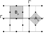
Figure 1: The surface code. Physical qubits are shown as black dots. The stabilizer operators are products of four Pauli operators, $A_{S}$ and $B_{P}$. Logical operators are correspond to string of Pauli operators crossing the qubit lattice from one side to the opposite, $\Gamma$ and $\Gamma^{\prime}$.

The physical qubits in the surface code are arranged on the edges of a square lattice, forming themselves a square lattice slanted by 45^o. The QEC scheme is based on the stabilizer formalism NC00-a with two sets of stabilizer: plaquettes

$$B_{P}=\prod_{i\in P}\sigma_{i}^{z},$$ (1)

and stars

$$A_{S}=\prod_{i\in S}\sigma_{i}^{x},$$ (2)

operators, as shown in Fig. (1).

When all stabilizers are enforced, the lattice of physical qubits in Fig. 1 encodes one logical qubit. The logical bit flip operator, $\bar{X}$, is the product of physical bit flip operators, $\sigma^{x}$, along a path from the upper to the lower sides of the lattice, e.g., through path $\Gamma$ in Fig. (1). Similarly, a logical phase flip operator, $\bar{Z}$, is the product of physical phase flips operators,$\sigma^{z}$, joining the vertical boundaries of the lattice, e.g., path $\Gamma^{\prime}$, in Fig. 1.

Additional logical qubits can be encoded in the same set of physical qubits by relaxing the stabilizers constrains PhysRevA.86.032324 . However, the case of a single logical qubit is expected to have the largest possible threshold. Hence, we focus on this situation and define the logical states as

$$|\bar{\uparrow}\rangle=\frac{1}{\sqrt{N_{\lozenge}}}G|F\rangle$$ (3)

and

$$|\bar{\downarrow}\rangle=\bar{X}|\bar{\uparrow}\rangle,$$ (4)

where $|F\rangle$ is the ferromagnetic $z$ state of the physical qubits, $N_{\lozenge}$ is a normalization constant, $G=\prod_{\lozenge}\left(1+A_{\lozenge}\right)$, and $\prod_{\lozenge}$ is the product over all star stabilizers.

II.2 Environment

The traditional “system plus environment” approach to open quantum systems RevModPhys1987 ; CaldeiraBook is the most natural method to systematically study memory effects and spatial correlations. In this approach, the environment is described by a large set of harmonic oscillators,

$$H_{0}=\sum_{{\bf k}}\omega_{{\bf k}}a_{{\bf k}}^{\dagger}a_{{\bf k}},$$ (5)

where $a_{\mathbf{k}}$ and $a_{\mathbf{k}}^{\dagger}$ are bosonic annihilation and creation operators that have the usual canonical commutation relations, i.e., $\left[a_{\mathbf{k}},a_{\mathbf{k^{\prime}}}^{\dagger}\right]=\delta_{\mathbf{k},\mathbf{k^{\prime}}}$, where we set $\hbar=1$. The environmental modes have momentum $k_{i}=\frac{2\pi}{L}$ $n_{i}$ with $n_{i}$ an integer and $L$ a macroscopic characteristic length. Finally, following our assumptions we consider the dispersion relation, $\omega_{{\bf k}}=v\left|{\bf k}\right|$.

The full quantum evolution is given by the Hamiltonian

$$H=H_{0}+V,$$ (6)

where $V$ is the interaction between the qubits and the environment. A pure bit-flip error model has the interaction Hamiltonian Weiss:1999:1 ; breuer2007theory ,

$$V=\lambda\sum_{{\bf r}}f\left(\mathbf{r}\right)\sigma_{{\bf r}}^{x},$$ (7)

where $f\left(\mathbf{r}\right)$ is the bosonic operator

$$f\left(\mathbf{r}\right)=\frac{\left(v/\omega_{0}\right)^{D/2+s}}{L^{D/2}}\sum_{\mathbf{k}\neq 0}\left|\mathbf{k}\right|^{s}\left(e^{+i\mathbf{k}\cdot\mathbf{r}}a_{\mathbf{k}}^{\dagger}+\mbox{H. c.}\right),$$ (8)

$\omega_{0}$ is a characteristic microscopic frequency scale, and $D$ the number of spatial dimensions of the environment. The power $s$ defines the low-frequency behavior of the enviroment’s spectral density, as we show below.

It is straightforward to derive the time evolution operator in the interaction picture after a time $\Delta$,

$$\hat{U}\left(\Delta,0\right)=T_{t}e^{-i\lambda\int_{0}^{\Delta}dt\sum_{\mathbf{r}}\hat{f}\left(\mathbf{r},t\right)\sigma_{\mathbf{r}}^{x}},$$ (9)

where

$$\hat{f}\left(\mathbf{r},t\right)=\frac{1}{L^{D/2}}\sum_{\mathbf{k}\neq 0}\left|\mathbf{k}\right|^{s}\left(e^{+i\mathbf{k}\cdot\mathbf{r}+i\omega_{k}t}a_{\mathbf{k}}^{\dagger}+e^{-i\mathbf{k}\cdot\mathbf{r}-i\omega_{k}t}a_{\mathbf{k}}\right),$$ (10)

and $T_{t}$ is the time ordering operator.

Although the dispersion relation of the environment is an important quantity, what traditionally defines the type of environment is its spectral density

$$J(\omega)\equiv\frac{\pi}{2}\sum_{k}\frac{C_{k}^{2}}{m_{k}\omega_{k}}\delta(\omega-\omega_{k}).$$ (11)

Here $C_{k}$ comes from the interaction term, Eq. (7), when it is written in the coordinate-coordinate coupling scheme, $V=q_{0}\sigma_{x}\sum_{k}C_{k}q_{k}$. In the latter, the length scale $q_{0}$ is introduced in such a way we recover the appropriate dimension of the interaction term. Usually, it comes from the original Hamiltonian of the system we are representing here as our physical qubits. For example, $\pm q_{0}$ could be the positions of two degenerate minima of a localized tunneling center breuer2007theory .

In order to identify $C_{k}$ for our model, we use Eqs. (7) and (8), and $q_{k}=\sqrt{1/2m_{k}\omega_{k}}(a_{k}+a_{k}^{\dagger})$. In this way we get:

$$C_{k}^{2}=2\lambda^{2}\frac{(v/\omega_{0})^{D+2s}}{q_{0}^{2}L^{D}}m_{k}vk^{2s+1}.$$ (12)

Now we can calculate the spectral density. We do this by inserting $C_{k}^{2}$ into Eq. (11), and taking the continuum limit (i.e. $\frac{(2\pi)^{D}}{L^{D}}\sum_{k}\rightarrow\int d^{D}k$). Finally we assume a two-dimensional environment, i.e. $D=2$, and perform the corresponding integration, obtaining:

$$J(\omega)=\frac{2\lambda^{2}}{q_{0}^{2}\omega_{0}^{2+2s}}\omega^{2s+1}.$$ (13)

Thus, following the standard definition, a two-dimensional environment with $s<0$ is known as subohmic, while for $s=0$ and $s>0$ they are known as ohmic and superohmic, respectively.

We can use some of the properties of Gaussian environments to simplify Eq. (10) arXiv:1606.0316 . We first use the Magnus expansion Blanes2009151 for the evolution operator to deal with the time ordering operator and then normal order the exponentials, finally arriving at

$$\hat{U}\left(\Delta,0\right)=\left[\prod_{{\bf k}\neq 0}e^{-\hat{{\cal G}}\left({\bf k},\Delta,0\right)}\,e^{-i\hat{\alpha}\left({\bf k},\Delta,0\right)a_{{\bf k}}^{\dagger}}e^{-i\hat{\alpha}^{*}\left({\bf k},\Delta,0\right)a_{{\bf k}}}\right],$$ (14)

where

$$\hat{\alpha}\left({\bf k},\Delta,0\right)=\frac{\lambda}{L^{D/2}}\int_{\Delta\left(n-1\right)}^{\Delta n}dt\sum_{\mathbf{r}}|\mathbf{k}|^{s}\hat{\sigma}_{\mathbf{r},n}^{x}e^{+i\mathbf{k}\cdot\mathbf{r}+i\omega_{k}t},$$ (15)

and

$$\hat{{\cal G}}\left({\bf k}\right) = -\frac{\lambda^{2}}{L^{D}}\left(v/\omega_{0}\right)^{D+2s}\int_{0}^{\Delta}dt_{1}\int_{0}^{\Delta}dt_{2}\theta\left(t_{1}-t_{2}\right)$$ (16)

$$\times\ \sum_{\mathbf{r},\mathbf{r^{\prime}}}\left|\mathbf{k}\right|^{2s}e^{-i\mathbf{k}\cdot\left(\mathbf{r}-\mathbf{r^{\prime}}\right)-i\omega_{k}\left(t_{1}-t_{2}\right)}\hat{\sigma}_{\mathbf{r}}^{x}\hat{\sigma}_{\mathbf{r^{\prime}}}^{x}.$$

A detailed derivation of these steps can be found in Ref. arXiv:1606.0316 .

For later convenience, we rewrite Eq. (14) in the qubit $x$ basis $\{|\pm\rangle\}$, where $\hat{\sigma}^{x}|\pm\rangle=\pm|\pm\rangle$. By defining $\left|\sigma\right\rangle$ as a configuration of qubits with eigenvalue $\sigma_{{\bf r}}^{x}=\pm 1$ for the qubit at position ${\bf r}$, we recast Eq. (14) as

$$\hat{U}\left(\Delta,0\right)=\sum_{\bar{\sigma}}u\left(\bar{\sigma}\right)\left|\bar{\sigma}\right\rangle\left\langle\bar{\sigma}\right|,$$ (17)

where $\bar{\sigma}=\{\sigma_{\mathbf{r}}^{x}\}$ denotes the full set of spin variables, the pure bosonic operator is defined as

$$u\left(\bar{\sigma}\right)=\prod_{{\bf k}\neq 0}e^{-{\cal G}\left({\bf k}\right)}\,e^{-i\alpha\left({\bf k}\right)\,a_{{\bf k}}^{\dagger}}\,e^{-i\alpha^{*}\left({\bf k}\right)\,a_{{\bf k}}},$$ (18)

and the auxiliary functions are given by

$${\cal G}\left({\bf k}\right) = -\frac{\lambda^{2}}{L^{D}}\left(v/\omega_{0}\right)^{D+2s}\int_{0}^{\Delta}dt_{1}\int_{0}^{\Delta}dt_{2}\theta\left(t_{1}-t_{2}\right)$$ (19)

$$\times\ \sum_{\mathbf{r},\mathbf{r^{\prime}}}\left|\mathbf{k}\right|^{2s}e^{-i\mathbf{k}\cdot\left(\mathbf{r}-\mathbf{r^{\prime}}\right)-i\omega_{k}\left(t_{1}-t_{2}\right)}\sigma_{\mathbf{r}}^{x}\sigma_{\mathbf{r^{\prime}}}^{x},$$

$$\alpha\left({\bf k},\Delta,0\right)=\frac{\lambda}{L^{D/2}}\int_{\Delta\left(n-1\right)}^{\Delta n}dt\sum_{\mathbf{r}}|\mathbf{k}|^{s}\sigma_{\mathbf{r},n}^{x}e^{+i\mathbf{k}\cdot\mathbf{r}+i\omega_{k}t}.$$ (20)

III Logical Qubit Fidelity

We initially set the system in the logical state $|\bar{\uparrow}\rangle$ and and assume that the environment is in its ground state $|0\rangle$,

$$|\psi_{0}\rangle=|\bar{\uparrow}\rangle\otimes|0\rangle.$$ (21)

We consider that the syndromes are extracted at equal time intervals of duration $\Delta$ and that the extraction is performed instantaneously. Hence, the full evolution operator is composed by a sequence of unitary evolutions and projections. In the simplest case of a nonerror syndrome, where there is no recovery operation to be performed, the quantum state after $N$ cycles is given by

$$|\psi\rangle = \mathcal{P}_{0}\,U\left(N\Delta,\left(N-1\right)\Delta\right)\ldots$$ (22)

$$\ldots\mathcal{P}_{0}\,U\left(2\Delta,\Delta\right)\mathcal{P}_{0}\,U\left(\Delta,0\right)|\psi_{0}\rangle,$$

where

$$\mathcal{P}_{0}=|\bar{\uparrow}\rangle\langle\bar{\uparrow}|+\bar{X}|\bar{\uparrow}\rangle\langle\bar{\uparrow}|\bar{X}.$$ (23)

We now introduce a subscript to the spin variable sets to designate the QEC step where the spin states evolve and use Eq. (17) to rewrite

$$|\psi\rangle = \sum_{\bar{\sigma}_{1}\ldots\bar{\sigma}_{N}}\left[u\left(\bar{\sigma}_{N}\right)\ldots u\left(\bar{\sigma}_{2}\right)\,u\left(\bar{\sigma}_{1}\right)\left|0\right\rangle\right]{\cal P}_{0}\left|\bar{\sigma}_{N}\right\rangle$$ (24)

$$\left\langle\bar{\sigma}_{N}\right|\mathcal{P}_{0}\left|\bar{\sigma}_{N-1}\right\rangle\ldots\left\langle\bar{\sigma}_{2}\right|\mathcal{P}_{0}\left|\bar{\sigma}_{1}\right\rangle\left\langle\bar{\sigma}_{1}|\bar{\uparrow}\right\rangle,$$

where $\sigma_{{\bf r}}^{x}\left|\bar{\sigma}_{n}\right\rangle=\sigma_{{\bf r},n}\left|\bar{\sigma}_{n}\right\rangle$ and $\sigma_{{\bf r},n}=\pm 1$. Since we have already integrated over time in Eqs. (19) and (20), these labels work now as new time variables.

The projectors can also be easily expressed in the $x$ basis of the qubits,

$$\mathcal{P}_{0}=\frac{1}{2^{M}N_{\lozenge}}\sum_{\bar{\sigma},\bar{\sigma}^{\prime}}\sum_{{\cal J}=\left\{\bar{I},\bar{X}\right\}}G{\cal J}|\bar{\sigma}\rangle\langle\bar{\sigma}^{\prime}|{\cal J}G$$ (25)

where $M$ the total number of qubits and $\left\{\bar{\sigma},\bar{\sigma}^{\prime}\right\}$ are two independent sum of all qubit configurations in the $x$ basis. After relabeling the indexes and using the property $G^{2}=N_{\lozenge}G$, we obtain

$$|\psi\rangle = \frac{1}{\sqrt{{\cal N}}}\sum_{\left\{\bar{\sigma}_{i},{\cal J}_{i}\right\}}\left[\prod_{n=0}^{N-1}u\left(\bar{\sigma}_{n}\right)\left|0\right\rangle\right]$$ (26)

$$\times\,{\cal J}_{N-1}\,G\left|\bar{\sigma}_{N-1}\right\rangle\prod_{n=0}^{N-2}\left\langle\bar{\sigma}_{n}\right|{\cal J}_{n}\,G\left|\bar{\sigma}_{n}\right\rangle$$

with ${\cal N}$ being a normalization constant and ${\cal J}_{i}=\left\{\bar{I},\bar{X}\right\}$.

When we use Eq. (26) to evaluate an expectation value, we have terms with the same “time” label coming from the ket and the bra. Hence, it is convenient to differentiate the origin of each term by renaming the variables in the bra $\left\langle\psi\right|$ as

$$\sigma \to\tau,$$

$$\alpha \to\beta,$$

$${\cal J} \to{\cal K}.$$

It is now straightforward to write the logical state fidelity after $N$ QEC cycles,

$$\mathcal{F}=\frac{\left\langle\psi|\bar{\uparrow}\right\rangle\left\langle\bar{\uparrow}|\psi\right\rangle}{\langle\psi|\psi\rangle},$$ (27)

where

$$\left\langle\psi|\bar{\uparrow}\right\rangle\left\langle\bar{\uparrow}|\psi\right\rangle = \frac{1}{{\cal N}}\sum_{\left\{\bar{\sigma}_{i},\bar{\tau}_{i}\right\}}\sum_{\left\{{\cal J}_{i},{\cal K}_{i}\right\}}^{\prime}$$ (28)

$$\times\,\left\langle 0\right|\left[\prod_{k=N-1}^{0}u^{\dagger}\left(\bar{\tau}_{k}\right)\right]\left[\prod_{j=0}^{N-1}u\left(\bar{\sigma}_{j}\right)\right]\left|0\right\rangle$$

$$\times\,\prod_{l=0}^{N-1}\left\langle\bar{\tau_{l}}\right|{\cal J}_{l}\,G\left|\bar{\tau}_{l}\right\rangle\left\langle\bar{\sigma}_{l}\right|{\cal J}_{l}\,G\left|\bar{\sigma}_{l}\right\rangle,$$

where $\sum^{\prime}$ denotes a summation with the restrictions $\mathcal{J}_{0}=\mathcal{K}_{0}=\mathcal{J}_{N-1}=\mathcal{K}_{N-1}=\bar{I}$. Similarly,

$$\langle\psi|\psi\rangle = \frac{1}{{\cal N}}\sum_{\left\{\bar{\sigma}_{i},\bar{\tau}_{i}\right\}}\sum_{\left\{{\cal J}_{i},{\cal K}_{i}\right\}}$$ (29)

$$\times\,\left\langle 0\right|\left[\prod_{k=N-1}^{0}u^{\dagger}\left(\bar{\tau}_{k}\right)\right]\left[\prod_{j=0}^{N-1}u\left(\bar{\sigma}_{j}\right)\right]\left|0\right\rangle$$

$$\times\,\prod_{l=0}^{N-1}\left\langle\bar{\tau}_{l}\right|{\cal J}_{l}\,G\left|\bar{\tau}_{l}\right\rangle\left\langle\bar{\sigma}_{l}\right|{\cal J}_{l}\,G\left|\bar{\sigma}_{l}\right\rangle,$$

but with no restrictions on $\mathcal{J}_{n}$ or $\mathcal{K}_{n}$. Notice $\langle\psi|\psi\rangle\neq 0$ in general, since the time evolution of the system is non-unitary.

To further simplify these expressions, we normal order the expectation value of the bosonic operators. This is a tedious task, but easily performed using the Baker-Campbell-Hausdorff formula. For instance,

$$e^{-i\alpha^{*}({\bf k},n)\,a_{{\bf k}}}\,e^{-i\alpha({\bf k},m)\,a_{{\bf k}}^{\dagger}} = e^{-i\alpha({\bf k},m)\,a_{{\bf k}}^{\dagger}}\,e^{-i\alpha^{*}({\bf k},n)\,a_{{\bf k}}}$$ (30)

$$\times\,e^{-\alpha^{*}({\bf k},n)\,\alpha({\bf k},m)}.$$

After performing several commutations to normal order the bosonic operators, we obtain

$$\left\langle 0\right|\left[\prod_{k=N-1}^{0}u^{\dagger}\left(\bar{\tau}_{k}\right)\right]\left[\prod_{j=0}^{N-1}u\left(\bar{\sigma}_{j}\right)\right]\left|0\right\rangle = \prod_{{\bf k}\neq 0}\exp\left\{-\sum_{n=0}^{N-1}\left[{\cal G}({\bf k},n)+{\cal G}^{*}({\bf k},n)-\beta^{*}({\bf k},n)\,\alpha({\bf k},n)\right]\right\}$$ (31)

$$\times\,\exp\left\{-\ \sum_{n=1}^{N-1}\sum_{m=0}^{n-1}\left[\alpha^{*}({\bf k},n)\,\alpha({\bf k},m)+\beta({\bf k},n)\,\beta^{*}({\bf k},m)\right.\right.$$

$$\left.\left.-\ \beta^{*}({\bf k},n)\,\alpha({\bf k},m)-\alpha({\bf k},n)\,\beta^{*}({\bf k},m)\right]\right\}.$$

It is natural to rewrite this equation in the short and suggestive form of an exponential,

$$\left\langle 0\right|\left[\prod_{k=N-1}^{0}u^{\dagger}\left(\bar{\tau}_{k}\right)\right]\left[\prod_{j=0}^{N-1}u\left(\bar{\sigma}_{j}\right)\right]\left|0\right\rangle = e^{-{\cal H}},$$ (32)

where

$${\cal H} = \sum_{{\bf r},{\bf s}}\Big{\{}\sum_{n=0}^{N-1}F_{1}({\bf r}-{\bf s},0)\,(\tau_{{\bf r},n}-\sigma_{{\bf r},n})(\tau_{{\bf s},n}-\sigma_{{\bf s},n})$$ (33)

$$+\ i\Phi_{1}({\bf r}-{\bf s})\,(\tau_{{\bf s},n}-\sigma_{{\bf s},n})(\tau_{{\bf r},n}+\sigma_{{\bf r},n})+i\Phi_{2}({\bf r}-{\bf s},0)(\tau_{{\bf s},n}\sigma_{{\bf r},n}-\tau_{{\bf r},n}\sigma_{{\bf s},n})$$

$$-\ \sum_{n=1}^{N-1}\sum_{m=0}^{n-1}\left[F_{1}({\bf r}-{\bf s},n-m)-\Phi_{3}({\bf r}-{\bf s},n-m)\right](\tau_{{\bf r},n}-\sigma_{{\bf r},n})(\tau_{{\bf s},m}-\sigma_{{\bf s},m})$$

$$+\ i\left[F_{2}({\bf r}-{\bf s},n-m)+\Phi_{3}({\bf r}-{\bf s},n-m)\right](\tau_{{\bf r},n}-\sigma_{{\bf r},n})(\tau_{{\bf s},m}+\sigma_{{\bf s},m})\Big{\}},$$

and

$$F_{1}({\bf r},n) = \frac{\lambda^{2}(v/\omega_{0})^{D+2s}}{L^{D}}\sum_{{\bf k}\neq 0}\left|{\bf k}\right|^{2s}\left[\frac{1-\cos(\omega_{k}\Delta)}{\omega_{k}^{2}}\right]\cos({\bf k}\cdot{\bf r})\cos(n\omega_{k}\Delta),$$ (34a)

$$F_{2}({\bf r},n) = \frac{\lambda^{2}(v/\omega_{0})^{D+2s}}{L^{D}}\sum_{{\bf k}\neq 0}\left|{\bf k}\right|^{2s}\left[\frac{1-\cos(\omega_{k}\Delta)}{\omega_{k}^{2}}\right]\cos({\bf k}\cdot{\bf r})\sin(n\omega_{k}\Delta),$$ (34b)

$$\Phi_{1}({\bf r},n) = \frac{\lambda^{2}(v/\omega_{0})^{D+2s}}{L^{D}}\sum_{{\bf k}\neq 0}\left|{\bf k}\right|^{2s}\left[\frac{\omega_{k}\Delta-\sin(\omega_{k}\Delta)}{\omega_{k}^{2}}\right]\cos({\bf k}\cdot{\bf r}),$$ (34c)

$$\Phi_{2}({\bf r},n) = \frac{\lambda^{2}(v/\omega_{0})^{D+2s}}{L^{D}}\sum_{{\bf k}\neq 0}\left|{\bf k}\right|^{2s}\left[\frac{1-\cos(\omega_{k}\Delta)}{\omega_{k}^{2}}\right]\sin({\bf k}\cdot{\bf r})\cos(n\omega_{k}\Delta),$$ (34d)

$$\Phi_{3}({\bf r},n) = \frac{\lambda^{2}(v/\omega_{0})^{D+2s}}{L^{D}}\sum_{{\bf k}\neq 0}\left|{\bf k}\right|^{2s}\left[\frac{1-\cos(\omega_{k}\Delta)}{\omega_{k}^{2}}\right]\sin({\bf k}\cdot{\bf r})\sin(n\omega_{k}\Delta).$$ (34e)

Equation (33) can be interpreted as a statistical mechanics Hamiltonian of a three-dimensional lattice of Ising variables. The three dimensions are due to the the two-dimensional spatial lattice of the qubits and the discrete “time” direction. The different correlation functions originated from the bosonic model produce interactions between these Ising variables that can be long or short ranged.

Using this notation, the logical qubit fidelity can be cast as

$$\mathcal{F}=\frac{\sum^{\prime}_{\bar{\sigma},\bar{\tau}}e^{-{\cal H}}\prod_{l}\left\langle\bar{\tau}_{l}\right|{\cal J}_{l}\,G\left|\bar{\tau}_{l}\right\rangle\left\langle\bar{\sigma}_{l}\right|{\cal J}_{l}\,G\left|\bar{\sigma}_{l}\right\rangle}{\sum_{\bar{\sigma},\bar{\tau}}e^{-{\cal H}}\prod_{l}\left\langle\bar{\tau}_{l}\right|{\cal J}_{l}\,G\left|\bar{\tau}_{l}\right\rangle\left\langle\bar{\sigma}_{l}\right|{\cal J}_{l}\,G\left|\bar{\sigma}_{l}\right\rangle}.$$ (35)

There are two aspects to consider when analyzing this expression. First, the sum over the Ising variables in the numerator is constrained to the positive stars due to the projector $G$. Hence, not all Ising configurations of three dimensional lattice contribute to the sums. Second, the “energy cost” imposed by ${\cal H}$ assign different weights to the terms of the sum. Because of exchange symmetry $\sigma\leftrightarrow\tau$, these contributions are always real (but very difficult to evaluate).

In Sec. IV we evaluate the fidelity for a particularly set of environment parameters that allow for an analytical solution.

IV Superohmic environment with $s=1/2$

A very interesting case to consider has $s=1/2$ and $D=2$. This corresponds to a superohmic environment where analytical expressions for the correlations functions in Eqs. (34) can be easily written by imposing the continuum limit PhysRevA.88.012336

$$\frac{\left(2\pi\right)^{2}}{L^{2}}\sum_{\mathbf{k}}\rightarrow\int_{0}^{\Lambda}\rho\,d\rho\int_{0}^{2\pi}d\theta.$$

As usual when dealing with superohmic environments, some values for the variables ${\bf r}$ and $n$ in Eqs. (34) can lead to ultraviolet diverging contributions. The leading divergent terms are linearly proportional to the ultraviolet cutoff,

$$F_{1}(0,0)\approx\frac{\lambda^{2}v\Lambda}{2\pi\omega_{0}^{3}},$$ (36)

and

$$F_{1}\left(0,1\right)\approx-\frac{\lambda^{2}v}{2\pi\omega_{0}^{3}}\frac{\Lambda}{2},$$ (37)

with the remaining terms giving subleading contributions diverging with the cutoff or no divergence at all. Hence, for a large environmental cutoff, in leading order, it is a good approximation to simplify Eq. (33) to

$$\mathcal{H} \approx \frac{J}{4}\sum_{n=0}^{N-1}\sum_{\mathbf{r}}\Big{[}\left(\tau_{\mathbf{r},n}-\sigma_{\mathbf{r},n}\right)\left(\tau_{\mathbf{r},n}-\sigma_{\mathbf{r},n}\right)$$ (39)

$$+\ \frac{1}{2}\left(\tau_{\mathbf{r},n}-\sigma_{\mathbf{r},n}\right)\left(\tau_{\mathbf{r},n+1}-\sigma_{\mathbf{r},n+1}\right)\Big{]},$$

where $J=\frac{2\lambda^{2}v}{\pi\omega_{0}^{3}}\Lambda$.

We can now introduce the spin-1 operator

$$S_{{\bf r},n}\equiv\frac{1}{2}(\tau_{{\bf r},n}-\sigma_{{\bf r},n}),$$ (40)

and write

$$\mathcal{H}\approx J\sum_{n=0}^{N-1}\sum_{\mathbf{r}}\left(S_{{\bf r},n}^{2}+\frac{1}{2}S_{{\bf r},n}\,S_{{\bf r},n+1}\right),$$ (41)

which can be interpret as the Hamiltonian of decoupled spin-1 chains along the “time” direction of the statistical mechanics model associated to the fidelity calculation.

The first term in Eq. (41), $S_{{\bf r},n}^{2}$, is a “zero-field splitting” (also known as on-site anisotropy) and competes with the exchange coupling, $S_{{\bf r},n}S_{{\bf r},n+1}$. The physics of this statistical mechanical model is well known Capel1966 , and for the numerical prefactors on the right-hand side of Eq. (41) there is no phase transitions and no magnetic ordering. This means that the qubit configurations between QEC cycles do not energetically constrain each other in the calculation of the evaluating the fidelity through Eq. (35). Hence, we can find the threshold by discussing the critical coupling in a single QEC cycle. This result provides a more rigorous justification for the usual assumption that for a superohmic environment memory and correlations induced by the environment can be neglected in the evaluation of the threshold.

The fidelity can be evaluated as

$$\mathcal{F}=\frac{\sum^{\prime}_{\bar{\sigma},\bar{\tau}}\prod_{l}e^{-{\cal H}_{l}}\left\langle\bar{\tau}_{l}\right|{\cal J}_{l}\,G\left|\bar{\tau}_{l}\right\rangle\left\langle\bar{\sigma}_{l}\right|{\cal J}_{l}\,G\left|\bar{\sigma}_{l}\right\rangle}{\sum_{\bar{\sigma},\bar{\tau}}\prod_{l}e^{-{\cal H}_{l}}\left\langle\bar{\tau}_{l}\right|{\cal J}_{l}\,G\left|\bar{\tau}_{l}\right\rangle\left\langle\bar{\sigma}_{l}\right|{\cal J}_{l}\,G\left|\bar{\sigma}_{l}\right\rangle},$$ (42)

where the single-chair Hamiltonian is given by

$${\cal H}_{l}=J\,S_{{\bf r},l}^{2}.$$ (43)

Although there is no explicit interaction between the spin-1 variables, the constrain of positive stars make the evaluation of the fidelity nontrivial. The simplest method to deal with the constraint is to use “mass field variables” PhysRevA.90.042315 ; arXiv:1606.0316 . The mass field $\mu$ is an Ising variable defined in the center of each plaquette. The variable $\sigma_{{\bf r}}$ in the link between two plaquettes is written as the product of the mass field of each plaquette. For example, for bulk sites in Fig. 2,

$$\sigma_{\mathbf{r},l}=\mu_{\mathbf{x},l}\,\mu_{\mathbf{y},l}$$ (44)

and

$$\tau_{\mathbf{r},l}=\nu_{\mathbf{x},l}\,\nu_{\mathbf{y},l}.$$ (45)

We can now replace the sum over the constrained $\sigma$ and $\tau$ variables for an unconstrained sum over $\mu$ and $\nu$ variables.

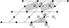
Figure 2: Illustration of mass field variables in the bulk and in the boundary for the spin variable $\sigma$.

The only issue remaining are the top and bottom lattice boundaries lattice. Stars located at the boundary are formed by only three qubits, but because of the positive stars constraint the mass field variables at these boundaries always assume the same value PhysRevA.90.042315 ,

$$\mu_{\mathbf{p}^{\prime},l}\,\sigma_{\mathbf{r}^{\prime},l}=\mu_{\mathbf{p}^{\prime\prime},l}\,\sigma_{\mathbf{r}^{\prime\prime},l}:=\alpha_{l}=\pm 1$$ (46)

and

$$\nu_{\mathbf{p}^{\prime},l}\,\tau_{\mathbf{r}^{\prime},l}=\nu_{\mathbf{p}^{\prime\prime},l}\,\tau_{\mathbf{r}^{\prime\prime},l}:=\beta_{l}=\pm 1.$$ (47)

Using the new variables, Eq. (43) can be rewritten as

$$\mathcal{H}_{l} = -\frac{J}{4}\Bigg{(}\sum_{\left\langle\mathbf{p},\mathbf{p^{\prime}}\right\rangle\in\text{bulk}}\nu_{\mathbf{p},l}\,\nu_{\mathbf{p^{\prime}},l}\,\mu_{\mathbf{p},l}\,\mu_{\mathbf{p^{\prime}},l}$$ (48)

$$+\ \sum_{\mathbf{p}\in\text{boundary}}\alpha_{\mathbf{p},l}\,\nu_{\mathbf{p},l}\,\mu_{\mathbf{p},l}\Bigg{)},$$

with no restrictions on the values of the mass field variables. We can further simplify the problem by noticing that the change of variables

$$s_{\mathbf{p},l}=\nu_{\mathbf{p},l}\,\mu_{\mathbf{p},l}$$ (49)

maps Eq. (48) into a square lattice Ising model with boundary fields arXiv:1606.0316

$$\mathcal{H}_{l}=-\frac{J}{4}\left(\sum_{\left\langle\mathbf{p},\mathbf{p^{\prime}}\right\rangle\in\text{bulk}}s_{\mathbf{p},l}\,s_{\mathbf{p^{\prime}},l}+\alpha_{l}\,\beta_{l}\sum_{\mathbf{p}\in\text{boundary}}s_{\mathbf{p},l}\right).$$ (50)

Following our previous work on this model and on the surface code fidelity calculation PhysRevA.90.042315 ; arXiv:1606.0316 and using the Onsager solution PhysRev.65.117 , we know that this model has a second-order phase transition at the critical coupling

$$J_{c}=2\ln\left(1+\sqrt{2}\right).$$ (51)

Thus, for $J>J_{c}$ the Ising model is in its ordered phase and the fidelity is smaller than unity. Conversely, for $J<J_{c}$ the Ising model is in its paramagnetic phase and the fidelity is unity PhysRevA.90.042315 ; arXiv:1606.0316 . Thus, the critical coupling constant for the surface code in this superohmic environment is

$$\lambda_{c}\approx 2\sqrt{\frac{\pi\omega_{0}^{3}}{v\Lambda}\ln\left(1+\sqrt{2}\right)}.$$ (52)

V Summary and Conclusions

There is a large body of theoretical work where the efficiency of QEC is analyzed. One of the most common methods employed is the use of the operator norm for the interaction Hamiltonian. However, this method is inapplicable to models with diverging norms, such as the spin-boson Terhal:2005:012336 ; AGP06 ; AKP06 . An alternative method is to use a master equation for the quantum evolution of the reduced density matrix, $\rho_{r}$ Weiss:1999:1 . Even though the master equation formalism is very general, some very stringent assumptions must be made even in the simplest cases in order to obtain workable expressions. In addition, the initial step of the formalism is to integrate the environmental degrees of freedom. Hence, it explicitly precludes any correlations induced by the environment between qubits at different QEC steps. In this paper we followed a third route: the Feynman-Vernon influence functional formalism Weiss:1999:1 .

We followed the full quantum evolution of the system and the environment and only at the end of the QEC evolution we traced the environment. For a single QEC step, both the influence functional formalism and a well-performed Lindblad description are expected to yield similar results. However, due to the syndrome extraction procedure, this equivalence may not hold when many QEC cycles are considered.

For a pure bit-flip model, it was possible to write the exact time evolution operator and then obtain an exact closed form for a logical qubit fidelity after an arbitrary number of QEC cycles, Eq. (35). Even for this simple pure bit-flip model the expression is daunting. For the surface code it corresponds to a three-dimensional lattice of interacting Ising variables that are constrained by the nature of the QEC code. This result can be understood in terms of a fictitious statistical mechanical problem NMB07 ; Novais:2008:012314 . In this language, the QEC threshold corresponds to a “phase transition”, where the system-environment coupling is mapped onto an effective inverse temperature. For a very small coupling (corresponding to a high-temperature phase) the statistical mechanical problem is in its disorder phase and QEC is able to keep the fidelity equal to unity. However, for large couplings (corresponding to a low-temperature phase) the qubits can “order” and the fidelity becomes smaller than unity.

We specialized the calculation for the superohmic case with $s=1/2$ and a two-dimensional environment. Superohmic environments are plagued with ultraviolet divergencies in some of the correlation functions that yield interactions between qubits. In the particular example of $s=1/2$ the leading diverging terms have a linear dependence with the ultraviolet cutoff. Although we peformed an explicit calculation for this particular value of $s$, similar results also hold for any $s>0$ case. Therefore, the discussions of Sec. IV can be extended for all superohmic cases.

In Sec. IV we demonstrated that the statistical mechanical problem defined by Eq. (35) can be simplified in the superohmic case to an array of spin-1 chains, Eq. (41). The particular set of parameters that emerged from the calculation tells us that the array is in a phase where the “zero-field splitting” term is dominant. Hence, the model can be further simplified and only this “zero-field splitting” term need to be kept. This analysis justifies the use of stochastic error models in the discussion of the QEC threshold for superohmic environments. The model has an analytical solution, allowing us to find an expression for the critical coupling where the threshold takes place, Eq. (52).

In summary, we provided and exact expression for the fidelity of a logical qubit in the surface code in the presence of a bosonic environment after an arbitrary number of QEC steps. We demonstrated that for superohmic environments the use of stochastic models is fully justifiable, thus confirming in an explicitly example an old conjecture of the literature NMB10 .

VI Acknowledgments

Daniel López acknowledges CNPq for financial support. A.O.C. and E. Novais wish to thank CNPq and FAPESP through the initiative INCT-IQ. This work was supported in part by the FAPESP Grant 2014/26356-9 and the NSF Grant CCF-1117241.

References

- (1) D. P. DiVincenzo, Phys. Scr. T137, 014020 (2009).
- (2) G. Waldherr et al., Nature (London) 506, 204 (2014).
- (3) D. A. Lidar and T. A. Brun, eds., Quantum Error Correction (Cambridge University Press, 2013).
- (4) S. Bravyi, M. B. Hastings, and S. Michalakis, J. Math. Phys. 51, 093512 (2010).
- (5) A. G. Fowler, M. Mariantoni, J. M. Martinis, and A. N. Cleland, Phys. Rev. A 86, 032324 (2012).
- (6) E. Novais, E. R. Mucciolo, and H. U. Baranger, Phys. Rev. Lett. 98, 040501 (2007).
- (7) H. K. Ng and J. Preskill, Phys. Rev. A 79, 032318 (2009).
- (8) E. Novais and E. R. Mucciolo, Phys. Rev. Lett. 110, 010502 (2013).
- (9) J. Preskill, Q. Info. Comp. 13, 181 (2013).
- (10) S. B. Bravyi and A. Y. Kitaev, arXiv:quant-ph/9811052v1 (1998).
- (11) E. Dennis, A. Kitaev, A. Landahl, and J. Preskill, J. Math. Phys. 43, 4452 (2002).
- (12) A. G. Fowler, A. M. Stephens, and P. Groszkowski, Phys. Rev. A 80, 052312 (2009)
- (13) P. Sarvepalli and R. Raussendorf, in Theory of Quantum Computation, Communication, and Cryptography, Lecture Notes in Computer Science, Vol. 6519, ed. by W VanDam, W and V. M. Kendon, and S. Severini, 2011, pp. 47-62.
- (14) A. G. Fowler, A. C. Whiteside, and L. C. L. Hollenberg, Phys. Rev. Lett. 108, 180501 (2012).
- (15) P. Jouzdani, E. Novais, and E. R. Mucciolo, Phys. Rev. A 88, 012336 (2013).
- (16) P. Jouzdani, E. Novais, I. S. Tupitsyn, and E. R. Mucciolo, Phys. Rev. A 90, 042315 (2014).
- (17) C. G. Brell, S. Burton, G. Dauphinais, S. T. Flammia, and D. Poulin, Phys. Rev. X 4, 031058 (2014).
- (18) E. Novais, A. Stanforth, and E. R. Mucciolo, arXiv:1606.03163 (2016).
- (19) E. Novais, E. R. Mucciolo, and H. U. Baranger, Phys. Rev. A 82, 020303 (2010).
- (20) M. A. Nielsen and I. L. Chuang, Quantum Computation and Quantum Information (Cambridge University Press, Cambridge UK, 2000).
- (21) E. Novais, E. Mucciolo, and H. U. Baranger, Phys. Rev. A 78, 012314 (2008).
- (22) D. P. DiVincenzo and P. Aliferis, Phys. Rev. Lett. 98, 020501 (2007).
- (23) G. Duclos-Cianci and D. Poulin, Phys. Rev. Lett. 104, 050504 (2010).
- (24) A. O. Caldeira and A. J. Leggett, Ann. Phys. 149, 374 (1983).
- (25) H. Breuer and F. Petruccione, The Theory of Open Quantum Systems (Oxford University Press, Oxford, 2007).
- (26) A. O. Caldeira, An Introduction to Macroscopic Quan- tum Phenomena and Quantum Dissipation (Cambridge University Press, 2014).
- (27) S. Vorojtsov, E. R. Mucciolo, and H. U. Baranger, Phys. Rev. B 71, 205322 (2005).
- (28) A. J. Leggett et al., Rev. of Mod. Phys. 59, 1 (1987).
- (29) S. Weiss, Quantum Dissipative Systems, 2nd ed. (World Scientific, Cambridge, UK, 1999).
- (30) S. Blanes, F. Casas, J. Oteo, and J. Ros, Phys. Rep. 470, 151 (2009).
- (31) H. W. Capel, Physica 32, 966 (1966).
- (32) L. Onsager, Phys. Rev. 65, 117 (1944).
- (33) B. M. Terhal and G. Burkard, Phys. Rev. A 71, 012336 (2005).
- (34) P. Aliferis, D. Gottesman and J. Preskill, Quant. Inf. Comp. 6, 97 (2006).
- (35) D. Aharonov, A. Kitaev, and J. Preskill, Phys. Rev. Lett. 96, 050504 (2006).