Exact solution of the Einstein-Skyrme model in a Kantowski-Sachs spacetime

Andronikos Paliathanasis anpaliat@phys.uoa.gr Instituto de Ciencias Físicas y Matemáticas, Universidad Austral de Chile, Valdivia, Chile    Michael Tsamparlis mtsampa@phys.uoa.gr Faculty of Physics, Department of Astronomy-Astrophysics-Mechanics University of Athens, Panepistemiopolis, Athens 157 83, Greece
Abstract

We consider a Skyrme fluid with a constant radial profile in locally rotational Kantowski-Sachs spacetime. The Skyrme fluid is an anisotropic fluid with zero heat flux and with an equation of state parameter $w_{S}$ that $\left|w_{s}\right|\leq\frac{1}{3}$. From the Einstein field equations we define the Wheeler-DeWitt equation. For the last equation we perform a Lie symmetry classification and we determine the invariant solutions for the wavefunction of the model. Moreover from the Lie symmetries of the Wheeler-DeWitt equation we construct Noetherian conservation laws for the field equations which we use in order to write the solution in closed form. We show that all pf the cosmological parameters are expressed in terms of the scale factor of the two dimensional sphere of the Kantowski-Sachs spacetime. Finally from the application of Noether’s theorem for the Wheeler-DeWitt equation we derive conservation laws for the wavefunction of the universe.

Cosmology; Skyrme fluid; Lie symmetries
pacs:
98.80.-k, 95.35.+d, 95.36.+x

I Introduction

The Skyrme model has various applications in physics (for instance see ref1 ; ref2 ; ref3 ; ref4 ; ref5 ). The model which was proposed by Skyrme in the early of 60s Skyrme1 ; Skyrme2 is a nonlinear theory of pions in which the baryons can be interpreted as topological soliton solutions of the model in the configuration space TopSol . The Skyrme field has been used as a sourced fluid in General Relativity, the so-called Einstein-Skyrme model. It has been shown that the Einstein-Skyrme model admits static black hole solutions with a regular event horizon which approaches asymptotically the Schwarzschild solution; furthermore, the Einstein-Skyrme model violates the “no hair” conjecture for black holes bh01 ; bh02 ; bh03 ; Ioannidou .

Recently the study of the dynamical evolution of the field equations of the Einstein-Skyrme model with a cosmological constant in a locally rotational  Kantowski-Sachs spacetime was performed in Parisi . In particular for the Skyrme fluid a constant radial profile oon the hedgehog Ansatz has been considered111For a discussion of the hedgehod ansatz on spherically symmetric spacetime and some generalizations see Canfora ; Canfora2 ; Canfora3 . and it has been shown that the field equations admit two stable point solutions. The two solutions describe an exponential scale factor for the

two-dimensional sphere of the Kantowski-Sachs spacetime. For a nonconstant radial profile, numerical solutions of the Einstein-Skyrme model in anisotropic cosmologies have been studied in Canfora4 . Specifically, in Canfora4 , the Einstein-Skyrme model was studied in Bianchi I and in Kantowski-Sachs universes and it has been found that bounds on the values of the cosmological constant and on the Skyrme coupling should be taken in order for solutions to exist.

In this work we consider the Einstein-Skyrme model with a constant radial profile and show that the Wheeler-DeWitt (WdW) Equation can be solved explicitly by means of the use of Lie point symmetries. Furthermore, following the method which was established in AB for scalar field cosmology with a matter source, we determine Noetherian conservation laws for the field equations. The existence of the new conservation laws implies that the field equations are Liouville integrable and with the method of separation of variables we write the analytical solution of the model.

Lie and Noether point symmetries are powerful tools which have been used for the study of various models in gravitational physics and cosmology. The symmetry analysis of charged perfect fluids in spherically symmetric spacetimes can be found in Maharaj1 ; Maharaj3 ; MahLeach . On the other hand Noether’s Theorem has been applied in various cosmological models in order to constrain the unknown functions in scalar-field cosmology, in $f\left(R\right)$ gravity, in $f\left(T\right)$ gravity and others ( see deRiti ; KotsakisL ; VakF ; dimakisT ; dimakisT2 ; Dib ; Hwei ; PalFR and references therein). The plan of the paper is as follows.

In Section II we consider our model which is General Relativity with a cosmological constant in a locally rotational Kantowski-Sachs spacetime where the matter source is a Skyrme fluid. For that model we write the field equations and we derive the WdW Equation. The existence of Lie point symmetries for the WdW equation and the invariant solutions are given in Section III. In Section IV we follow the method which was established in AB and we use the Lie point symmetries of the WdW Equation in order to study the Liouville integrability of the field equations. We construct the closed-form classical solution of the model, and we show that the cosmological parameters can be written in terms of the scale factor of the two-dimensional sphere, while the quantum potential is calculated. Finally, in Section V we draw our conclusions.

II Einstein-Skyrme Action

Consider the Einstein-Skyrme Action

$$S=\int dx^{4}\sqrt{-g}\left(R-2\Lambda\right)+S_{K},$$ (1)

in a Kantowski-Sachs background with line element

$$ds^{2}=-dt^{2}+A^{2}\left(t\right)dr^{2}+B^{2}\left(t\right)\left(d\theta^{2}+\sin^{2}\theta d\phi^{2}\right).$$ (2)

Spacetime (2) is a locally rotational spacetime (LRS) and admits a four-dimensional Killing algebra. In  particular, it admits as Killing vectors the Lie group $SO\left(3\right)$ plus the Killing vector $\partial_{r}$.

The term, $S_{K},$ in the total action (1) is the action of the Skyrme field

$$S_{K}=\frac{K}{2}\int dx^{4}\sqrt{-g}\left(\frac{1}{2}R_{\mu}R^{\mu}+\frac{\lambda}{16}F_{\mu\nu}F^{\mu\nu}\right),$$ (3)

where $R_{\mu}=U^{-1}U_{;\mu}$ $F_{\mu\nu}=\left[R_{\mu},R_{\nu}\right]$ and $U\left(x^{\mu}\right)$ is the $SU\left(2\right)$-valued scalar; finally $K~{}$and$~{}\lambda$ are positive constants Canfora ; TopSol .

Variation with respect to the metric in (1) provides us with the gravitational field equations

$$G_{\mu\nu}+\Lambda g_{\mu\nu}=kT_{\mu\nu},$$ (4)

in which $G_{\mu\nu}$ is the Einstein tensor $k$ is the Einstein constant, and $T_{\mu\nu}$ is the energy-momentum tensor for the Skyrme fluid. Furthermore variation with respect to the field $U\left(x^{\mu}\right)$ in (1) provides the matter conservation law $T_{~{};\nu}^{\mu\nu}=0$ which is

$$g^{\mu\nu}\left(R_{\mu;\nu}+\frac{\lambda}{4}\left(\left[R^{\sigma},F_{\sigma\nu}\right]\right)_{;\nu}\right)=0.$$ (5)

Following Canfora ; Parisi we consider the hedgehog Ansatz in which the radial profile function is constant and, specifically, $\frac{\pi}{2}+\sigma\pi,\sigma\in\mathbb{Z},$ where equation (5) is satisfied indentically, and the remaining system comprises the gravitational field equations (4) and now the energy-momentum tensor, $T_{\mu\nu},$ has the following nonzero components Canfora ; Parisi

$$T_{\theta}^{\theta}=T_{\phi}^{\phi}=\frac{K\lambda}{2B^{4}}$$ (6)

and

$$T_{t}^{t}=T_{r}^{r}=-\frac{K}{B^{2}}\left(1+\frac{\lambda}{2B^{2}}\right).$$ (7)

We recall that in the 1+3 analysis defined by the four-velocity $u^{a}$ the energy-momentum tensor is decomposed as follows

$$T_{\mu\nu}=\rho_{S}u_{\mu}u_{\nu}+p_{s}h_{\mu\nu}+q_{(\mu}u_{\nu)}+\pi_{\mu\nu},$$

where

$\displaystyle\rho_{S}$ $\displaystyle=T_{\mu\nu}u^{\mu}u^{\nu}~{},~{}p_{S}=\frac{1}{3}h^{\kappa\lambda}T_{\kappa\lambda},$ (8)
$\displaystyle q^{\mu}$ $\displaystyle=h^{\mu\kappa}T_{\kappa\nu}u^{\nu}~{},~{}\pi_{\mu\nu}=(h_{\mu}^{\kappa}h_{\nu}^{\lambda}-\frac{1}{3}h_{\mu\nu}h^{\kappa\lambda})T_{\kappa\lambda}$ (9)

and

$$h_{\mu\nu}=g_{\mu\nu}+u_{\mu}u_{\nu}$$ (10)

is the $u^{a}$ projective tensor. The variables, $\rho_{S},p_{S},q^{\mu},\pi_{\mu\nu},$ are the dynamical variables of the

energy-momentum tensor and represent respectively the mass density, the isotropic pressure, the heat flux and the traceless stress tensor, as measured by the observer $u^{\mu}$. Using this general result from (6), (7) we have that $q^{\mu}=0$,

$$\rho_{S}=\frac{1}{B^{2}}\left(\bar{k}+\frac{\mu}{2B^{2}}\right)~{},~{}p_{S}=-\frac{1}{3B^{2}}\left(\bar{k}-\frac{\mu}{2B^{2}}\right)$$ (11)

and

$$\pi_{\mu\nu}=diag\left(0,-\frac{2}{3}\rho_{S},\frac{1}{3}\rho_{S},\frac{1}{3}\rho_{S}\right),$$ (12)

where the new constants $\bar{k}~{}$and$~{}\mu~{}$are given by the relations $\bar{k}=kK$ and $\mu=\bar{k}\lambda.$

We define the equation-of-state parameter, $w_{S},$ for the Skyrme fluid as follows

$$w_{S}=\frac{p_{S}}{\rho_{S}}=-\frac{1}{3}\frac{\bar{k}B^{2}-\mu}{\bar{k}B^{2}+\mu}.$$ (13)

We note that, when $\bar{k}B>\mu$ and $w_{S}\simeq-\frac{1}{3},$ the fluid acts as a curvature-like component, whereas for $\bar{k}B^{2}<<\mu$ and $w_{S}\simeq\frac{1}{3}$ and the Skyrme fluid has the equation-of-state parameter of a radiation-like fluid. It follows that the equation-of-state parameter for the Skyrme fluid is bounded as follows

$$-\frac{1}{3}\leq w_{S}\leq\frac{1}{3}.$$ (14)

II.1 Minisuperspace approach

From the Action-integral, (1), and for the spacetime with line element, (2), we find that the Lagrangian of the field equations is given by the following expression

$$L\left(A,B,\dot{A},\dot{B}\right)=2B\dot{A}\dot{B}+A\dot{B}^{2}+AB^{2}\Lambda+A\left(\bar{k}-1\right)+\frac{A\bar{k}\lambda}{2B^{2}}$$ (15)

and that the field equations, (4), are Parisi :

$$2\frac{\dot{A}\dot{B}}{AB}+\frac{\dot{B}^{2}}{B^{2}}+\frac{1}{B^{2}}-\Lambda=\frac{1}{B^{2}}\left(\bar{k}+\frac{\mu}{2B^{2}}\right),$$ (16)
$$2\frac{\ddot{B}}{B}+\frac{\dot{B}^{2}}{B^{2}}+\frac{1}{B^{2}}-\Lambda=\frac{1}{B^{2}}\left(\bar{k}+\frac{\mu}{2B^{2}}\right)$$ (17)

and

$$\frac{\ddot{A}}{A}+\frac{\ddot{B}}{B}+\frac{\dot{A}\dot{B}}{AB}-\Lambda=-\frac{\mu}{2B^{4}}.$$ (18)

Moreover, for the lapse time $dt=N\left(\tau\right)d\tau$, the Lagrangian of the field equations (15) becomes

$$L\left(N,A,B,\dot{A},\dot{B}\right)=\frac{1}{N}\left(2BA^{\prime}B^{\prime}+AB^{\prime 2}\right)+N\left(AB^{2}\Lambda+\omega A+\mu\frac{A}{2B^{2}}\right),$$ (19)

where now the new constant $\omega$ is $\omega=\bar{k}-1.$ In this a case the field equations can be seen as the Euler-Lagrange equations with respect to the variables $\left\{N,A,B\right\}~{}$Ray .

In the minisuperspace approach the WdW Equation is defined as follows Will ; Hall ,

$$\hat{H}\Psi=0,$$ (20)

where $\hat{H}$ is the Hamiltonian operator defined by the conformal Laplace operator.

From the Lagrangian (19) we can define the momenta, $p_{A}$and $p_{B},$ as

$$p_{A}=\frac{2}{N}BB^{\prime}~{}~{},~{}~{}p_{B}=\frac{2}{N}\left(BA^{\prime}+AB^{\prime}\right).$$ (21)

Hence the Hamiltonian function is

$$H\equiv N\left[-\frac{A}{4B^{2}}p_{A}^{2}+\frac{1}{2B}p_{A}p_{B}-\left(AB^{2}\Lambda+\omega A+\mu\frac{A}{2B^{2}}\right)\right]=0.$$ (22)

Therefore under normal quantization, $p_{i}\sim\frac{\partial}{\partial x^{i}}$, from the Hamiltonian (22) and equation (20) we derive the WdW Equation222Recall that for the field equations (16)-(18) the minisuperspace has dimension two.

$$W\left(A,B,\Psi,\Psi_{B},\Psi_{,AA},\Psi_{,BB},\Psi_{,AB}\right)\equiv 0,$$ (23)

where $W$ is

$$W\equiv-\frac{A}{4B^{2}}\Psi_{,AA}+\frac{1}{2B}\Psi_{,AB}-\frac{1}{4B^{2}}\Psi_{,A}-\left(AB^{2}\Lambda+\omega A+\mu\frac{A}{2B^{2}}\right)\Psi$$ (24)

and $\Psi=\Psi\left(A,B\right)$ is the wavefunction of the universe. We observe that as the dimension of the minisuperspace is two in the WdW Equation, (23), there is no quantum correction term, i.e., the Ricci Scalar of the minisuperspace is an extra potential term.  Furthermore we remark that only the geometric degrees of freedom, i.e., $\left\{A,B\right\}$ are quantized and not the $SU\left(2\right)$ field from the Skyrme-fluid. This is because the Skyrme-fluid  is expressed on terms of the parameters, $\left\{A,B\right\}$, and there is not another degree of freedom which has been introduced from the Skyrme-fluid as we have considered that the radiation profile in the hedgehog Ansatz is constant.

In order to solve equation (24) we apply the method of group invariant transformations, specifically the Lie point symmetries. Recently in AB it has been shown that the existence of Lie point symmetries for the WdW Equation is related with oscillatory terms in the wave function of the universe. Furthermore, the existence of Lie point symmetries means that the classical field equations admit Noetherian conservation laws which can lead to the integrability of the field equation.  In the following Section we proceed with the determination of the Lie point symmetries for the WdW Equation, (23), and with the application of Lie invariants in order to construct analytical solutions of the wavefunction $\Psi\left(A,B\right)$. Analytical solutions of equation (23) without the Skyrme term can be found in Conradi ; Lopez .

III Point symmetries and invariant solutions for the WdW equation

The WdW Equation (23) is a second-order partial differential equation with independent variables $\left\{A,B\right\}$ and dependent variable $\Psi$. By definition the generator

$$\mathbf{X}=\xi^{A}\left(A,B,\Psi\right)\partial_{A}+\xi^{B}\left(A,B,\Psi\right)\partial_{B}+\eta\left(A,B,\Psi\right)\partial_{\Psi},$$ (25)

of a one-parameter point transformation on the space of variables $\left\{A,B,\Psi\right\}$ is called a Lie point symmetry of the differential equation $W$ when there exist a function $\lambda$ such that the following condition holds Bluman

$$\mathbf{X}^{\left[2\right]}W=\lambda W,~{}$$ (26)

where $X^{\left[2\right]}$ is the second prolongation/extension of $\mathbf{X}$ in the space $\left\{A,B,\Psi,\Psi_{,A},\Psi_{,B}\right\}$.

The symmetry condition, (26) provides a polynomial system on the derivatives of $\Psi$ the solution of which gives the unknown functions $\xi^{A},\xi^{B}$ and $\eta.~{}$Moreover, because (23) is a linear second-order partial differential equation of dimension two, the field (25) has the following form

$$\mathbf{X}=\mathbf{\xi}+\left(a_{0}\Psi+b\left(A,B\right)\right)\partial_{\Psi},$$ (27)

where $b\left(A,B\right)$ is a solution of the original equation and $\mathbf{\xi}=\xi^{A}\left(A,B\right)\partial_{A}+\xi^{B}\left(A,B\right)\partial_{B}.$

From condition (26) for the WdW Equation (23) we find the following Lie point symmetries,

$$X_{\Psi}=\Psi\partial_{\Psi}~{},~{}X_{b}=b\partial_{\Psi}~{},~{}X_{1}=\frac{1}{AB}\partial_{A},$$ (28)
$$X_{2}=\frac{B}{4\Lambda B^{4}+4\omega B^{2}+2\mu}\left(-A\partial_{A}+2B\partial_{B}\right)$$ (29)

and

$$X_{3}=\left(\frac{2AB^{2}\left(3\omega+2\Lambda B^{2}\right)}{3\left(2\Lambda B^{4}+2\omega B^{2}+\mu\right)}\partial_{A}-\frac{\left(2\Lambda B^{4}+6\omega B^{2}-3\mu\right)B}{3\left(2\Lambda B^{4}+2\omega B^{2}+\mu\right)}\partial_{B}\right),$$ (30)

with nonzero Lie Brackets $\left[X_{1},X_{3}\right]=X_{1},~{}\left[X_{2},X_{3}\right]=-X_{2}$. The vector fields, $X_{\Psi},X_{b},$ are trivial symmetries and reflect that the differential equation, $W,$ is linear333The Lie point symmetry $X_{\Psi}$ is called linear symmetry, and $X_{b}$ express the infinity number of solutions..

The existence of a (nontrivial) Lie symmetry vector for the second-order partial differential equation, $W$, means that there exists a coordinate transformation, $\left\{A,B\right\}\rightarrow\left\{\bar{A},\bar{B}\right\}$, in which equation $W$ is independent of one of the independent variables $\left\{\bar{A},\bar{B}\right\},~{}$i.e., $\frac{\partial W}{\partial\bar{A}}=0$ or $\frac{\partial W}{\partial\bar{B}}=0$, or equivalently, that there exists a coordinate transformation $\left\{A,B,\Psi\right\}\rightarrow\left\{\bar{A},\bar{B},\bar{\Psi}\right\},$ in which the partial differential equation, $W$, reduces to an ordinary differential equation444In general a partial differential equation with $l-$dependent variables is reduced to a differential equation of $\left(l-1\right)$-dependent variables.. Solutions which follow from the application of the Lie point symmetries are called invariant solutions.

The application of the Lie point symmetry, $Y_{1}=X_{1}+m_{1}X_{\Psi},~{}m_{1}\in\mathbb{C},$ to (23) gives that

$$\Psi_{1}\left(A,B\right)=\exp\left(\frac{m_{1}}{2}A^{2}B\right)\Phi\left(B\right),$$ (31)

where $\Phi\left(B\right)$ satisfies the following ordinary differential equation

$$m_{1}B^{2}\Phi_{,B}-\left(2B^{4}\Lambda+2\omega B^{2}+\mu\right)=0.$$ (32)

Hence we find that the invariant solution which follows from the application of the symmetry vector $Y_{1}$ is

$$\Psi_{1}\left(A,B\right)=\Psi_{1}^{0}\exp\left(\frac{2\Lambda B^{4}+6\omega B^{2}-3\mu}{3m_{1}B}+\frac{1}{2}m_{1}A^{2}B\right)$$ (33)

for $m_{1}\neq 0,~{}$and $\Psi_{1}\left(A,B\right)=0$, for $m_{1}=0$.

Similarly, from the symmetry vector, $Y_{2}=X_{1}+m_{2}X_{\Psi}$ $m_{2}\in\mathbb{C},$ we find that the invariant solution is of the form

$$\Psi_{2}\left(A,B\right)=\exp\left(-\frac{m_{2}}{6B}\left(2\Lambda B^{4}+6\omega B^{2}-3\mu\right)\right)\bar{\Phi}\left(C\right)~{},~{}C=A^{2}B,$$ (34)

where $\Phi\left(C\right)$ is given by the following equation

$$m_{2}\bar{\Phi}_{,C}+\bar{\Phi}=0.$$ (35)

Hence the invariant solution is,

$$\Psi_{2}\left(A,B\right)=\Psi_{2}^{0}\exp\left(-\frac{m_{2}}{6B}\left(2\Lambda B^{4}+6\omega B^{2}-3\mu\right)\right)\exp\left(-\frac{A^{2}B}{m_{2}}\right)$$ (36)

for $m_{2}\neq 0$, and $\Psi_{2}\left(A,B\right)=0$, for $m_{2}=0$.

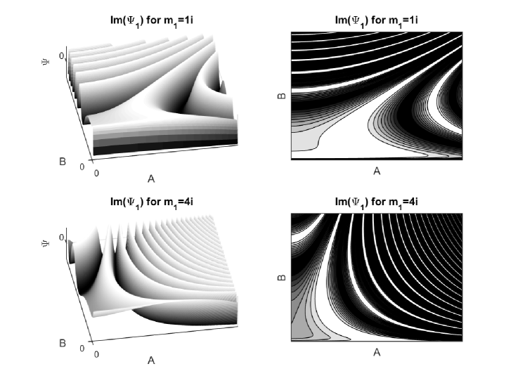
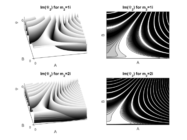
In Figs. 1 and 2 the qualitative evolution of the imaginary part of the wavefunction for the invariant solutions, $\Psi_{1}\left(A,B\right)$ and $\Psi_{2}\left(A,B\right)$, are given respectively for two different values of the constants $m_{1}~{}$and $m_{2}$. For the figures we considered the values $\Lambda=1$, $\omega=-0.5$ and $\mu=0.2$. From the figures the oscillatory behaviour of the wavefunction, which is related to the existence of Lie symmetries, can be observed.

Refer to caption
Figure 1: Evolution of the invariant solution $\operatorname{Im}\left(\Psi_{1}\right)~{}$of (33) which corresponds to the Lie point symmetry $Y_{1}$, for $m_{1}=1i$, and, $m_{1}=4i$. The plots are in the plane $A,B$, for $\Lambda=1$, $\omega=-0.5$ and $\mu=0.2$.
Refer to caption
Figure 2: Evolution of the invariant solution $\operatorname{Im}\left(\Psi_{2}\right)~{}$of (34) which corresponds to the Lie point symmetry $Y_{2}$, for $m_{2}=1i$, and, $m_{2}=2i$. The plots are in the plane $A,B$, for $\Lambda=1$, $\omega=-0.5$ and $\mu=0.2$.

From the Lie symmetry vector, $Y_{12}=X_{1}+cX_{2}+\gamma X_{\Psi}$, we have the invariant solution

$$\Psi_{12}\left(A,B\right)=\exp\left(-\frac{\gamma}{c}\frac{2B^{4}\Lambda+6\omega B^{2}-3\mu}{6B}\right)\Phi^{\prime}\left(C^{\prime}\right)$$ (37)

in which $\Phi^{\prime}\left(C^{\prime}\right)$ satisfies the second-order differential equation

$$2\Phi_{,C^{\prime}C^{\prime}}^{\prime}-\gamma\Phi_{,C^{\prime}}^{\prime}-c\Phi^{\prime}=0,$$ (38)

where $C^{\prime}=\frac{3}{\gamma B}\left(2B^{4}\Lambda+6\omega B^{2}-3\mu+3cA^{2}B^{2}\right)$. Hence we have that

$$\Psi_{12}=\exp\left(-\frac{\gamma}{c}\frac{2B^{4}\Lambda+6\omega B^{2}-3\mu}{6B}\right)\left(\Psi_{12}^{0}\exp\left(\gamma_{+}C^{\prime}\right)+\Psi_{12}^{{}^{\prime}0}\exp\left(\gamma_{-}C^{\prime}\right)\right),$$ (39)

where $\gamma_{\pm}=\frac{1}{4}\left(\gamma\pm\sqrt{\gamma^{2}+8c}\right)$.

Furthermore from the Lie symmetry vector, $Y_{13}=cX_{1}+X_{3}+3mX_{\Psi}$,$~{}m\in\mathbb{C}$, we find the invariant solution

$$\Psi_{13}\left(A,B\right)=\left(\Psi_{13}^{0}I_{m}\left(\frac{\sqrt{6}}{3}\bar{A}\bar{B}\right)+\Psi_{13}^{0\prime}K_{m}\left(\frac{\sqrt{6}}{3}\bar{A}\bar{B}\right)\right)\left(\frac{\bar{A}}{\bar{B}}\right)^{-m},$$ (40)

where $I_{m},~{}K_{m}$ are the modified Bessel functions of the first and second kind respectively.

Furthermore from the symmetry vector $Y_{23}=cX_{2}+X_{3}+3mX_{\Psi}$ $m\in\mathbb{C},$ the following invariant solution follows

$$\Psi_{23}\left(A,B\right)=\left(\frac{AB}{\bar{C}}\right)^{m}\left(\Psi_{23}^{0}I_{m}\left(\frac{\sqrt{6}}{3}A\bar{C}\right)+\Psi_{23}^{0^{\prime}}K_{m}\left(\frac{\sqrt{6}}{3}A\bar{C}\right)\right),$$ (41)

where $\left(\bar{C}\right)=\left(2\Lambda B^{4}+6\omega B^{2}+2cB-3\mu\right)^{1/2}$.

Finally from the generic symmetry vector, $Y_{G}=c_{1}X_{1}+c_{2}X_{2}+X_{3}+3mX_{\Psi}$, we have the following invariant solution

$$\Psi_{G}\left(A,B\right)=\left(\Psi_{G}^{0}I_{m}\left(\sqrt{2}iA^{\prime}B^{\prime}\right)+\Psi_{G}^{\prime 0}K_{m}\left(\sqrt{2}iA^{\prime}B^{\prime}\right)\right)\left(\frac{A^{\prime}}{B^{\prime}}\right)^{m_{3}},$$ (42)

where

$$A^{\prime}=\sqrt{3BA^{2}+2c_{1}}$$ (43)

and

$$B^{\prime}=\frac{1}{3}B^{-\frac{1}{2}}\left(2\Lambda B^{4}+6\omega^{2}B^{2}+2c_{2}B-3\mu\right)^{\frac{1}{2}}\text{.}$$ (44)

We remark that, as equation (24) is a linear equation, the general solution is expressed as a linear combination of all the Lie invariant solutions for all the values of the free parameters, that is

$$\Psi_{Total}\left(A,B\right)={\displaystyle\sum\limits_{m_{1}}}a_{m_{1}}\Psi_{1}\left(A,B\right)+{\displaystyle\sum\limits_{m_{2}}}b_{m_{2}}\Psi_{2}\left(A,B\right)+...$$ (45)

In the following Section we proceed with the derivation of the analytical solution for the classical field equations (16)-(18).

IV Classical Solution

As we discussed in Section II, the existence of a Lie point symmetry for the WdW Equation, (23), is equivalent with the existence of a Noetherian conservation law for the field equation. It is easy to see that the Lagrangian, (15), does not admit any Noether symmetries apart from the autonomous one. However, for specific lapse, $N$, the conformally related Lagrangian (19) admits as Noether symmetries the Lie point symmetries of equation (23) (for details see IJGMMP ).

For instance, when $N\left(A,B\right)=A^{-1}$, the vector field, $X_{1},$ is a Noether symmetry of (19) and the corresponding conservation law is $I_{1}=\dot{B}$.  The Hamiltonian, (22), and the conservation law are in involution, i.e., $\left\{H,I_{1}\right\}=0$, which means that the dynamical system which describes the field equations is Liouville integrable.

Similarly for different lapse, $N$, the other vector fields, i.e. $X_{2},X_{3}$, or any linear combination, produce Noetherian conservation laws. On the other hand, as the solution is unique and the field equations are conformally invariant the analytical solution that we find can be transformed into different lapse functions, $N$.

Under the coordinate transformation,

$$A=\sqrt{\frac{2x}{y}},~{}B=y,$$ (46)

the Lagrangian, (19), of the field equations becomes

$$L=\frac{\sqrt{2}}{2N}\sqrt{\frac{y}{x}}x^{\prime}y^{\prime}+N\sqrt{2}\sqrt{\frac{x}{y}}\left(\omega+\Lambda y^{2}+\frac{\mu}{2y^{2}}\right)$$ (47)

and the Hamiltonian

$$H\equiv N\sqrt{2}\sqrt{\frac{x}{y}}\left(\frac{1}{2}p_{x}p_{y}-\left(\omega+\Lambda y^{2}+\frac{\mu}{2y^{2}}\right)\right)=0.$$ (48)

Without loss of generality we select the lapse function $N\left(A,B\right)=A^{-1}=\sqrt{\frac{y}{2x}}$.  The line element of the spacetime, (2), becomes

$$ds^{2}=-\frac{1}{A^{2}\left(\tau\right)}d\tau^{2}+A^{2}\left(\tau\right)dr^{2}+B^{2}\left(\tau\right)\left(d\theta^{2}+\sin^{2}\theta d\phi^{2}\right).$$ (49)

Moreover, the Hamiltonian (48) of the field equations becomes

$$H\equiv\frac{1}{2}p_{x}p_{y}-\left(\omega+\Lambda y^{2}+\frac{\mu}{2y^{2}}\right)=0$$ (50)

and Hamilton’s equations are

$$x^{\prime}=\frac{1}{2}p_{y}~{},~{}y^{\prime}=\frac{1}{2}p_{x},$$ (51)

and

$$p_{x}^{\prime}=0~{},~{}p_{y}^{\prime}=2\Lambda y-\frac{\mu}{y^{3}}.$$ (52)

Equations (50)-(52) are the field equations for the model with the Action, (1).

The general solution of the field equations is ($I_{1}\neq 0$):

$$y\left(\tau\right)=\frac{I_{1}}{2}\tau+y_{0}$$ (53)
$$x\left(\tau\right)=\frac{I_{1}\Lambda}{12}\tau^{3}+\frac{\Lambda y_{0}}{2}\tau^{2}-\frac{2\mu}{I_{1}^{2}\left(I_{1}\tau+2y_{0}\right)}+x_{1}\tau+x_{0}$$ (54)

with constraint

$$x_{1}I_{1}-2\Lambda y_{0}^{2}-2\omega=0.$$ (55)

In the special case for which $I_{1}=0$ the solution is

$$x\left(\tau\right)=\frac{2\Lambda y_{0}^{4}-\mu}{4y_{0}^{3}}\tau^{2}+x_{1}\tau+x_{0}~{},~{}y\left(\tau\right)=y_{0},$$ (56)

where now the constraint equation which follows from (50) is

$$\omega+\Lambda y_{0}^{2}+\frac{\mu}{2y_{0}^{2}}=0$$ (57)

and so $\omega<0$. The last solution means that $B\left(t\right)=y_{0},$ that is, the fluid components, (11) and (12), of the Skyrme field are constants.

Hence from (46) we have that

$$A\left(\tau\right)=\sqrt{A_{0}\tau^{2}+2\frac{x_{1}}{y_{0}}\tau+2\frac{x_{0}}{y_{0}}},$$ (58)

where $A_{0}=\frac{2\Lambda y_{0}^{4}-\mu}{y_{0}^{4}}$, and, when $x_{1}=x_{0}=0,$ we have that $A^{2}\left(\tau\right)=A_{0}\tau^{2},$ whereas in the proper time, $N=1$, $A\left(t\right)=\sqrt{A_{0}}e^{\sqrt{A_{0}}t}$ which is a de Sitter behaviour. The latter solution holds only when $I_{1}=0$.  Hence a small perturbation of the solution gives that $I_{1}\neq 0$ and so the solution is unstable.

Concerning the solution with $I_{1}\neq 0$, from (46) and (53) we have that

$$\tau=\frac{2}{I_{1}}B-\frac{y_{0}}{I_{1}}.$$ (59)

Hence

$$x\left(B\right)=\frac{\Lambda}{12I_{1}^{2}}\left(2B-y_{0}\right)^{3}+\frac{\Lambda y_{0}}{2I_{1}^{2}}\left(2B-y_{0}\right)^{2}-\frac{\mu}{I_{1}^{2}B}+\frac{x_{1}}{I_{1}}\left(2B-y_{0}\right)+x_{0}$$ (60)

which means that $A\left(\tau\right)$ is expressed as a function of $B$, i.e. $A\left(B\right)$.

For the line element, (49), we can define the spatial volume $V=AB^{2}\sin\theta$ and the average scale factor $a=V^{\frac{1}{3}}~{}$Yadav . Therefore the average Hubble function, $H=A\frac{a^{\prime}}{a},$ is

$$H=\frac{1}{3}\left(A^{\prime}+2\frac{A}{B}B^{\prime}\right),$$ (61)

where $H_{A}=A^{\prime},~{}H_{B}=\frac{A}{B}B^{\prime}$ are the Hubble functions on the direction $r$ and on the two sphere $d\Omega^{2},$ respectively. However,

$$A^{\prime}=\frac{1}{A}\left(\frac{x^{\prime}}{y}-\frac{x}{y^{2}}y^{\prime}\right)=\left(\frac{x^{\prime}}{AB}-\frac{I_{1}}{4}\frac{A}{B}\right)$$ (62)

and $B^{\prime}=\frac{I_{1}}{2}$. Therefore equation (61) becomes

$$H=\frac{1}{3}\left(\frac{x^{\prime}}{AB}+\frac{I_{1}}{4}\frac{A}{B}\right),$$ (63)

where

$$\frac{dx\left(B\right)}{dB}=\frac{\Lambda}{4I_{1}}\left(2B-y_{0}\right)^{2}+\frac{\Lambda y_{0}}{I_{1}}\left(2B-y_{0}\right)+\frac{2\mu}{4I_{1}^{2}B^{2}}+x_{1}.$$ (64)

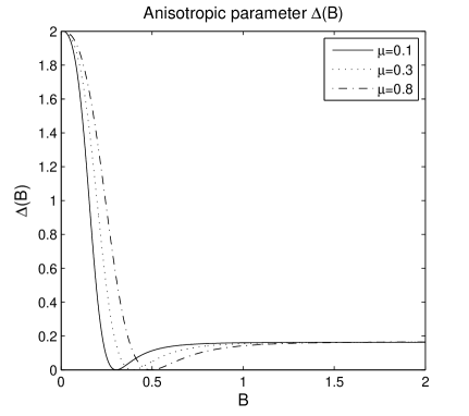
Finally the anisotropic parameter is defined as

$$\Delta\left(B\right)=\frac{\left(H_{A}-H\right)^{2}+2\left(H_{B}-H\right)^{2}}{3H^{2}}.$$ (65)

The evolution of the anisotropic parameter, $\Delta\left(B\right),$ can be found in fig. 3, where it is shown that the anisotropic parameter vanishes at a point and afterwards becomes a nonzero constant.

Refer to caption
Figure 3: Evolution of the anisotropic parameter $\Delta\left(B\right)$ for various values of the parameter $\mu$. We observe that the anisotropic parameter reach a minimum close to zero and after it becomes constant. For the plots we selected $A=0$ when $B=0$.

IV.1 Semiclassical Solution

The solution presented above is the classical solution of the field equations. Because the solution of the WdW equation is known we study the quantum effects in the classical behaviour which follow from the quantum potential  in the semiclassical approach of Bohmian mechanics boh1 ; boh2 . A method which has been applied recently in various models dimakisT2 ; TchRN ; manto ; Stu2 .

In particular, if the solution of the WDW equation is $\Psi\left(x^{k}\right)=A\left(x^{k}\right)e^{iB\left(x^{k}\right)}$, where now $A\left(x^{k}\right)$ is not a slow-roll function, then the substitution of that solution into the WDW equation gives

$$H\left(p_{k},x^{k}\right)+Q_{V}=0,$$ (66)

where $H\left(p_{k},x^{k}\right)$ is the Hamiltonian function which generates the WDW equation, $Q_{V}=\frac{\Delta\left(A\right)}{A},$ is the quantum potential and the momentum $p_{\mu}=\frac{\partial B\left(x^{k}\right)}{\partial x^{\mu}}$.  Equation (66) is the new Hamiltonian of the field equations which provides us with the semiclassical solution.  In the limit for which $Q_{V}=0$ or $A$ is a slow-roll function we are in the region of the WKB approximation if and only if $B\left(x^{k}\right)$ is a solution of the Hamilton-Jacobi equation for the classical field equations.

From the solution of the WdW Equation, (39), we can see that the quantum potential is zero and we are in the classical solution. Consider now the wavefunction (41) and $\Psi_{23}^{0\prime}=0$. The wavefunction is

$$\Psi\left(A,B\right)=\Psi_{23}^{0}\left(\frac{AB}{\bar{C}}\right)^{m}I_{m}\left(\frac{\sqrt{6}}{3}A\bar{C}\right).$$ (67)

In order to determine the quantum correction we have to extract from the wavefunction the nonoscillatory terms.  Let not $m=i\sigma$, $\sigma\in\mathbb{R}$, and we are in the region in which $A\rightarrow 0$ $B\rightarrow 0,~{}$ such that $B<<\mu,$ which gives that $\bar{C}=i\left|\bar{C}\right|.~{}$Hence the solution (67) is approximated as follows

$$\Psi\left(A,B\right)\simeq\bar{\Psi}_{0}\exp\left[i\sigma\ln\left(AB\right)\right]\exp\left(-i\bar{\sigma}\ln\left(\left|\bar{C}\right|\right)\right)\left(A\left|\bar{C}\right|\right)^{\sigma},$$ (68)

which provides us with the quantum potential $Q_{V}=\frac{3\sigma^{2}\left(2\Lambda B^{4}+2\omega B^{2}+\mu\right)}{4AB^{2}}\left|\bar{C}\right|^{-2}$.  Here we note that, if $\bar{C}$ was a real function, then the quantum potential would be zero.  Furthermore from (68) we have the oscillatory term, $B\left(A,B\right)=\sigma\ln\left(AB\right)-\bar{\sigma}\ln\left(\left|\bar{C}\right|\right),$ from which we find that $p_{A}=\frac{\sigma}{A}~{},~{}p_{B}=\frac{\sigma}{B}+\frac{\bar{\sigma}\left(8\Lambda B^{3}+12\omega B-2c\right)}{2\bar{C}^{2}}$ and the reduced field equations are

$$\frac{2}{N}BB^{\prime}=\frac{\sigma}{A},$$ (69)
$$\frac{2}{N}BA^{\prime}=\frac{\bar{\sigma}\left(8\Lambda B^{3}+12\omega B-2c\right)}{2\bar{C}^{2}}.$$ (70)

If we consider that $N=A$, we have the solution

$$B^{2}\left(t\right)=2\sigma\left(\tau-\tau_{0}\right)$$ (71)

and

$$\ln\left(A\left(t\right)\right)=\int\frac{\bar{\sigma}\left(8\Lambda B^{3}+12\omega B-2c\right)}{2B\bar{C}^{2}}$$ (72)

which is different from the previous solution. Of course that solution holds only in the region of $A,B$ which we have already considered for the derivation of the quantum potential and specifically when $A\rightarrow 0$ $B\rightarrow 0,$ that is, quantum effects take place.

V Conclusions

In this work we considered a locally rotational Kantowski-Sachs spacetime with cosmological constant and a Skyrme fluid with constant radial profile. For the comoving observer the Skyrme fluid is an anisotropic fluid with zero heat flux component and nonzero stress tensor. Furthermore for the equation-of-state parameter, $w_{S},$ for the Skyrme fluid $\left|w_{s}\right|\leq\frac{1}{3}$ holds.

In order to construct the solution of the field equations we followed a method established in AB , that is, we derived the WdW Equation and we showed that it admits Lie point symmetries. The existence of the Lie point symmetries means that the wavefunction of the universe admits oscillatory terms which follow from the Lie invariants. Moreover, from the Lie point symmetries of the WdW Equation we constructed Noetherian conservation laws for the classical field equations and proved the Liouville integrability of the field equations We used the Noetherian conservation laws in order to derive the solution of the field equations. We have found two families of solutions, one in which the scale factor, $B$, of the two sphere, is not constant and one in which it is constant.  For the first solution we expressed the cosmological parameters in terms of the scale factor, $B$, and we derived the anisotropic parameter, $\Delta\left(B\right),$ and showed that for initial conditions $\lim\limits_{B\rightarrow 0}A\left(B\right)=0$ the anisotropic parameter reaches a minimum close to zero and for large values of $B$ becomes constant different than zero. For the second solution for which $B=const.$ we have shown that the scale factor, $A$, of the radius, has an exponential behaviour.

At this point we wish to compare our results with the solutions that have been found previously in Parisi . As we discussed above, in the latter work the authors performed a fixed point analysis of the gravitational field equations, (16)-(18), and they derived some special solutions which describe the solution of the field equations at the fixed point, i.e. for a

specific initial-value problem of the field equations. In this work the solutions that we have presented are the general solution of the system and that can be seen from the number of the constants of integration. If we consider the initial conditions to be that of the fixed points of the field equations, the special solution of Parisi is easily recovered. Furthermore the importance of this work is that the integrability of the field equations (16)-(18) is proved which means that a solution always exists, while integrability cannot proved by the fixed-point analysis. Only in the region of the fixed points can the solution be approximated from the linearized system. The integrability of the Einstein-nonlinear $\sigma$ models is still an open subject of special interest.

Before we conclude, we note that the WdW Equation (24) follows from a variational principle in which the Lagrangian for the WdW Equation is

$$\mathcal{L}\left(A,B,\Psi_{,A},\Psi_{,B}\right)=-\frac{A}{4B^{2}}\left(\Psi_{,A}\right)^{2}+\frac{1}{2B}\Psi_{,A}\Psi_{,B}+\frac{1}{2}\left(AB^{2}\Lambda+\omega A+\mu\frac{A}{2B^{2}}\right)\Psi^{2}.$$ (73)

In IJGMMP2 it has been shown that the nontrivial Lie point symmetries of the Klein-Gordon equation are also Noether symmetries. Hence from the Lie point symmetries, (28)-(30), and for the Lagrangian (73) we can construct conservation flows for the wavefunction of the universe. In particular, for the case in which the minisuperspace has dimension two, the Noetherian conservation flow is given by the expression $I^{i}=\xi^{k}H_{k}^{i}$ , and satisfies the condition $D_{i}I^{i}=0$, where

$$\mathcal{H}_{k}^{i}=\frac{1}{2}\left(\frac{\partial\mathcal{L}}{\partial\Psi_{,i}}\Psi_{,k}-\delta_{k}^{i}\mathcal{L}\right),$$ (74)

and, $D_{i}=\frac{\partial}{\partial x^{i}}+\Psi_{,i}\frac{\partial}{\partial\Psi}+\Psi_{,ij}\frac{\partial}{\partial\Psi_{j}}+$.

For the Lagrangian (73) we have that $x^{i}=\left(A,B\right)$. Hence the conservation flow which corresponds to the symmetry vector $X_{1},~{}X_{2},~{}X_{3}$ has the following components

$$\mathcal{I}^{A}\left(X_{1}\right)=-\frac{1}{2}\frac{\left(\Psi_{,A}\right)^{2}}{B^{3}}+\frac{V_{eff}}{AB}\Psi^{2}~{},~{}\mathcal{I}^{B}\left(X_{1}\right)=\frac{\left(\Psi_{,A}\right)^{2}}{AB^{2}},$$ (75)
$$\mathcal{I}^{A}\left(X_{2}\right)=\frac{\left(A\Psi_{,A}-2B\Psi_{,B}\right)^{2}-2AB^{2}V_{eff}\Psi^{2}}{\left(2\Lambda B^{4}+2\omega B^{2}+\mu\right)B}~{},~{}$$ (76)
$$\mathcal{I}^{B}\left(X_{2}\right)=\frac{4B^{2}V_{eff}\Psi^{2}}{\left(2\Lambda B^{4}+2\omega B^{2}+\mu\right)}$$ (77)

and

$$\mathcal{I}^{A}\left(X_{3}\right)=-\frac{\left(2\Lambda B^{4}+2\omega B^{2}+\mu\right)^{-1}}{2}\left[\begin{array}[c]{c}A\left(2\Lambda B^{2}+3\omega\right)\left(A\left(\Psi_{,A}\right)^{2}-B^{2}V_{eff}\Psi^{2}\right)+\\ +\left(2\Lambda B^{4}+6\omega B^{2}-3\mu\right)\left(\left(\Psi_{,B}\right)^{2}-AB^{-1}\Psi_{,A}\Psi_{,B}\right)\end{array}\right]$$ (78)
$$\mathcal{I}^{B}\left(X_{3}\right)=\frac{3}{4}\frac{A}{B}\left(\Psi_{,A}\right)^{2}-\frac{B}{2}\frac{\left(2\Lambda B^{4}+6\omega B^{2}-3\mu\right)}{\left(2\Lambda B^{4}+2\omega B^{2}+\mu\right)}V_{eff}\Psi^{2}$$ (79)

where $V_{eff}=\left(AB^{2}\Lambda+\omega A+\mu\frac{A}{2B^{2}}\right).$

Therefore, the existence of Lie point symmetries for the WdW equation is equivalent with the existence of Noetherian conservation laws for the latter equation.

A more general consideration of the Skyrme fluid with nonconstant radial profile Canfora4 will be of interest. Such an analysis is in progress and will be published in a forthcoming work.

Acknowledgements.
The research of AP was supported by FONDECYT grant no. 3160121.

References

  • (1) E. Witten and D. Olive, Phys. Lett. B 78 97 (1987)
  • (2) N. Nagaosa and Y. Tokura, Nature Nanotechnology 8 899 (2013)
  • (3) S. Banerjee, J. Rowland, O. Erten and M. Randeria, Phys. Rev. X 4 031045 (2014)
  • (4) V.G. Makhankov, Y.P. Rybanov and V.I. Sanyuk, The Skyrme Model: Fundamental Methods Applications, Springer-Verlag, Berlin Heidelberg (1993)
  • (5) K. Benson and M. Bucher, Nucl. Phys. B 406 355 (1993)
  • (6) T. Skyrme, Proc. R. Soc. London A 260 127 (1961)
  • (7) T. Skyrme, Nucl. Phys., 31 556 (1962)
  • (8) N. Manton and P. Sutcliffe, Topological Solitons, Cambridge University Press, New York, (2004)
  • (9) S. Droz, M. Heusler and N. Straumann, Phys. Lett. B 268 371 (1991)
  • (10) M. Heusler, S. Droz and N. Straumann, Phys. Lett. B 285 (1992)
  • (11) H. Luckock and I. Moss, Phys. Lett. B, 176 341 (1986)
  • (12) T. Ioannidou, B. Kleihaus and J. Kunz, Phys. Lett. B 643 213 (2006)
  • (13) L. Parisi, N. Radicella and G. Vilasi, Phys. Rev. D., 91 063533 (2015)
  • (14) F. Canfora and H. Maeda, Phys. Rev. D. 87 084049 (2013)
  • (15) F. Canfora, Phys. Rev. D 88 065028 (2013)
  • (16) F. Canfora and P. Salgado-Rebolledo, Phys. Rev. D 87 045023 (2013)
  • (17) F. Canfora, A. Giacomini and S.A. Pavluchenko, Phys. Rev. D 90 043516 (2014)
  • (18) M.P. Jr. Rayan, and L.C. Shepley, Homogeneous Relativistic Cosmologies, Princeton University Press, Princeton (1975)
  • (19) A. Paliathanasis, M. Tsamparlis, S. Basilakos and J.D. Barrow, Phys. Rev. D. 91 123535 (2015)
  • (20) M.C. Kweyama, K.S. Govinder and S.D. Maharaj, Class. Quantum Grav. 18 105005, (2011)
  • (21) M.C. Kewyama, K.S. Govinder, and S.D. Maharaj, J. Math. Phys., 53 033707 (2012)
  • (22) S.D. Maharaj, P.G.L. Leach and R. Maartens, Gen. Relativ. Gravit. 28 35 (1996)
  • (23) R. de Ritis, G. Marmo, G. Platania, C. Rubano, P. Scudellaro and C. Stornaiolo, Phys. Rev. D. 42 (1990) 1091
  • (24) S. Cotsakis, P.G.L. Leach and H. Pantazi, Grav. Cosm. 4 314 (1998)
  • (25) B. Vakili, Phys. Lett. B 669 209 (2008)
  • (26) N. Dimakis, T. Christodoulakis and P.A. Terzis, J. Geom. Phys. 77 97 (2014)
  • (27) P.A. Terzis, N. Dimakis and T. Christodoulakis, Phys. Rev. D. 90 123543 (2014)
  • (28) K. Atazadeh and F. Darabi, EPJC 72 1 (2012)
  • (29) H. Wei, X.J. Guo and L.F. Wang, Phys.Lett. B 707 298 (2012)
  • (30) A. Paliathanasis, M. Tsamparlis and S. Basilakos, Phys. Rev. D. 84 123514 (2011)
  • (31) D. Wiltshire, An introduction to quantum cosmology (2001) (arXiv: gr-qc/0101003);
  • (32) J.J. Halliwell, Introductory lectures on quantum cosmology (2009) (arXiv: 0909.2566 [gr-qc])
  • (33) H.D. Conradi, Class. Quantum Grav. 12 2423 (1995)
  • (34) J.C. López-Domínguez, O. Obregón, and S. Zacarías, Phys. Rev. D, 84, 024015 (2011)
  • (35) G.W. Bluman and S. Kumei, Symmetries of Differential Equations, Springer-Verlag, New York, (1989)
  • (36) A. Paliathanasis and M. Tsamparlis, Int. J. Geom. Meth. Mod. Phys., 11 1450037 (2014)
  • (37) A.K. Yadav, Astrophys.Space Sci. 335 565 (2011)
  • (38) D. Bohm, Phys. Rev. 55 (1952) 166
  • (39) D. Bohm, Phys. Rev. 85 (1952) 180
  • (40) T. Christodoulakis, N. Dimakis, P.A. Terzis, B. Vakili, E. Melas and T. Grammenos, Phys.Rev. D 89 044031 (2014)
  • (41) A. Zampeli, T. Pailas, P.A. Terzis and T. Christodoulakis, JCAP 05 066 (2016)
  • (42) F. Tovar Falciano, N. Pinto-Neto and W. Struyve, Phys. Rev. D 91 (2015) 043524
  • (43) A. Paliathanasis, M. Tsamparlis and M.T. Mustafa, Int. J. Geom. Meth. Mod. Phys., 12 1550033 (2015)