Filament actuation by an active colloid at low Reynolds number

Abstract

Active colloids and externally actuated semi-flexible filaments provide basic building blocks for designing autonomously motile micro-machines. Here, we show that a passive semi-flexible filament can be actuated and transported by attaching an active colloid to its terminus. We study the dynamics of this assembly when it is free, tethered, or clamped using overdamped equations of motion that explicitly account for active fluid flow and the forces it mediates. Linear states are destabilized by buckling instabilities to produce stable states of non-zero curvature and writhe. We demarcate boundaries of these states in the two-dimensional parameter space representing dimensionless measures of polar and apolar activity. Our proposed assembly can be used as a novel component in the design of micro-machines at low Reynolds number and to study elastic instabilities driven by “follower” forces.

I introduction

Autonomously actuated slender bodies provide the basic building blocks for super-diffusive transport at both the cellular and extra-cellular levels. Classic examples are flagella and cilia brennen1977fluid . Flagellar propulsion endows microorganisms and spermatozoa with motility while ciliary layers have diverse functions including the transport of mucous and other biological fluids lyons2006reproductive ; enuka2012epithelial . Such active transport keeps, for instance, the trachea free of dust and aids the transfer of ovum to the uterus. Ciliary dysfunction causes many human diseases lyons2006reproductive ; tilley2014cilia . It is conceivable that biomimetic ciliary layers may have therapeutic uses. Recent experiments have, in fact, been able to transport genetic material, therapeutic payloads and functionalized groups to a target using synthetic propulsion systems orozco2014bubble ; gao2014environmental ; jurado2015self ; singh2015nano ; orozco2015micromotors ; duan2015synthetic ; wang2013small . Enhanced mixing in the context of microfluidics has also been realized and has numerous technological applications guix2014nano ; singh2015nano . The design of autonomously motile micro-machines is now a vigorous field of research involving a close dialogue between experiment and theory camalet1999self ; golestanian2007designing ; masoud2012designing ; keaveny2013optimization ; williams2014self . Recent surveys of the state-of-the-art are provided in den2013microfluidic ; duan2015synthetic ; gao2014environmental .

In this work, we propose and theoretically analyse a novel mechanism of actuation of a slender body immersed in a viscous fluid in conditions where inertia is negligible. We show that a passive elastic filament can be actuated by attaching an active colloid to its terminus. The dynamics of a such an assembly is unexpectedly rich when the flow of the surrounding fluid and the forces it mediates are taken into account. We study the dynamics, when the other terminus is free, tethered or clamped, as a function of the leading modes of activity of the colloid. From this, we identify states of filament motion that are most suited for biomimetic tasks such as propulsion and mixing.

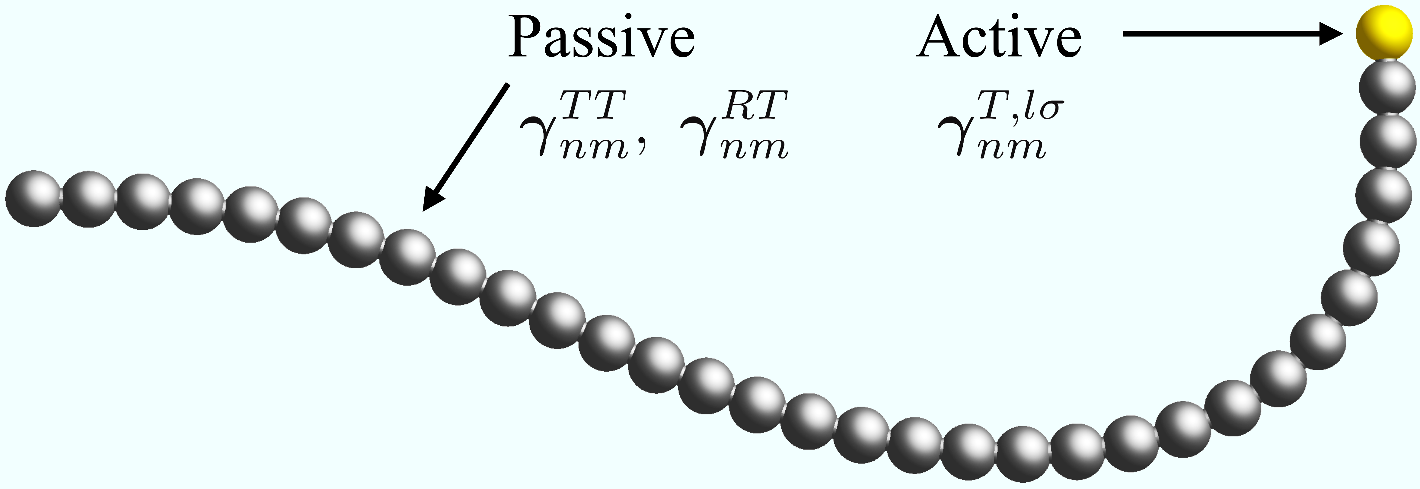
Figure 1: Schematic of a passive filament actuated by an active colloid attached to its terminus. The Stokes and slip friction coefficients indicate the nature of the hydrodynamic interaction between the passive beads of the filament and the active sphere (see text).

In recent work, Isele-Holder et al isele2016dynamics have analysed a converse situation, in which an active filament is attached to a passive colloid. Their study in two-dimensions neglects hydrodynamic interactions. The importance of hydrodynamic interactions in active systems is well-established marchetti2013hydrodynamics . In the present context, hydrodynamic interactions can induce instabilities in filaments that are stable in their absence, and must be considered in the energy balance that determines the efficiency of active transport. Our work includes the motion of the ambient fluid in which dynamics takes place and includes both the hydrodynamic interaction mediated by the fluid flow and the viscous dissipation that takes place in the fluid when computing transport efficiencies.

The theoretical aspect of our study builds on previous work in which overdamped stochastic equations of motion were derived for the motion of an active slender body that takes into account its elasticity, Brownian motion and active fluid flow laskar2015brownian . While the drift terms in the equations of motion were derived systematically from the solution of the Stokes equations for active spheres, the diffusion terms were included through a heuristic argument. Here, we develop the theory of Brownian motion with hydrodynamic interactions of a mixture of active and passive colloids in which both drift and diffusion terms are derived systematically. We recover the overdamped equations of laskar2015brownian when all particles of the mixture are active. The limit in which exactly one particle of the mixture is active provides a natural setting for analysing the dynamics of a passive filament (considered as a chain of passive particles) actuated by an active colloid, the main focus of this work.

The remainder of the paper is organized as follows. In the Section II we develop the theory of the hydrodynamically correlated Brownian motion of a mixture of active and passive spheres. In the Section III following procedure that is now classical doi1988theory , we use the theory of Brownian motion particles to construct equations of motion of filaments, consisting of a mixture of active and passive “beads”. In Section IV we take the limit of the above equations in which all but one particle is active and further restrict the activity to the two modes that produce the most dominant fluid flow. In Section V we perform a thorough numerical study of the resulting equations of motions and identify states of motion, in the parameter space spanned by the two dimensionless measures of activity, most suited for biomimetic applications. A linear stability analysis is performed to locate the values of these dimensionless measures at which the filament is actuated and to identify the nature of the dynamical instability through which this actuation is achieved. We conclude with a discussion and a summary in the section VI.

II Brownian microhydrodynamics of active and passive spheres

We consider $M$ passive spheres and $N-M$ active spheres, each of radius $a$, in an incompressible viscous fluid. The $n$-th sphere is centered at $\mathbf{R}_{n}$, oriented along $\mathbf{p}_{n}$, translating with linear velocity $\mathbf{V}_{n}$ and rotating with angular velocity $\bm{\Omega}_{n}$. The index $n$ runs through $1,\ldots,M,M+1,\ldots,N.$ While the velocity at a point on the boundary of a passive colloid is its rigid body motion, for an active colloid there is an additional active slip $\mathbf{v}^{\mathcal{A}}(\boldsymbol{\rho}_{n})$. These lead to the boundary conditions

$$\mathbf{v}(\mathbf{R}_{n}+\boldsymbol{\rho}_{n})=\begin{cases}\mathbf{V}_{n}+\boldsymbol{\Omega}_{n}\times\boldsymbol{\rho}_{n}&n\in\mathrm{passive},\\ \mathbf{V}_{n}+\boldsymbol{\Omega}_{n}\times\boldsymbol{\rho}_{n}+\mathbf{v}^{\mathcal{A}}(\boldsymbol{\rho}_{n})&n\in\mathrm{active},\end{cases}$$ (1)

which are basic to the mechanics of active and passive spheres. This method of modelling activity at the surface of the sphere by an additional velocity slip has been used earlier in the study of electrophoresis derjaguin1965molecular ; anderson1989colloid ; golestanian2007designing and in the case of ciliary propulsion of microbes blake1971spherical . The slip in all these studies was assumed to have azimuthal symmetry about the $\mathbf{p}_{n}$ axis. We differ from these earlier studies by choosing the most general form of the slip that is consistent with mass conservation ghose2014irreducible ; singh2014many .

The active slip velocity is conveniently parameterised by a series expansion in tensorial spherical harmonics $\mathbf{Y}^{(l)}$,

$$\mathbf{v}^{\mathcal{A}}\,(\bm{\rho}_{n})=\sum_{l=1}^{\infty}\frac{1}{(l-1)!(2l-3)!!}\mathbf{V}_{n}^{(l)}\cdot\mathbf{Y}^{(l-1)}(\bm{\hat{\rho}}_{n}).$$ (2)

Furthermore, the irreducibility of the tensorial harmonics implies that the expansion coefficients $\mathbf{V}_{n}^{(l)}$ are tensors of rank $l$, symmetric and irreducible in their last $l-1$ indices. By using this property, the coefficients can be decomposed into three irreducible tensors - $\mathbf{V}_{n}^{(ls)},\mathbf{V}_{n}^{(la)},\mathbf{V}_{n}^{(lt)}$ - of rank $l$, $l-1$ and $l-2$; they correspond to symmetric traceless, antisymmetric and trace combinations of the reducible indices. We denote the three irreducible parts by $\mathbf{V}^{(l\sigma)}$ and the suffixes $\sigma=s,a,t$ are self-explanatory singh2014many ; singh2016traction .

For convenience, we introduce special notations for the $l\sigma=1a$ and $l\sigma=2a$ coefficients. These, as will be clear below, are the linear and angular velocities of an isolated force-free, torque-free active sphere in an unbounded fluid. They are expressed as $4\pi a^{2}\mathbf{V}_{n}^{\mathcal{A}}=-\int\mathbf{v}^{\mathcal{A}}(\bm{\rho}_{n})dS_{n}$ and $4\pi a^{2}\bm{\Omega}_{n}^{\mathcal{A}}=-\frac{3}{2a^{2}}\int\bm{\rho}_{n}\times\mathbf{v}^{\mathcal{A}}(\bm{\rho}_{n})dS_{n}$.

In the absence of inertia, Newton’s equations for the spheres reduce to instantaneous balance of forces and torques,

$$\mathbf{F}_{n}^{H}+\mathbf{F}_{n}^{B}+\bm{\xi}_{n}^{T}=0,$$ (3)

$$\mathbf{T}_{n}^{H}+\mathbf{T}_{n}^{B}+\bm{\xi}_{n}^{R}=0.$$ (4)

Here, $\mathbf{F}_{n}^{H}$ and $\mathbf{T}_{n}^{H}$ are the contact forces and torques applied by the fluid, given by integrals of the force per unit area $\mathbf{f}=\bm{\sigma}\cdot\mathbf{\hat{\boldsymbol{\rho}}}_{n}$ on the boundary $S_{n}$ of the $n$-th sphere, where $\mathbf{\hat{\boldsymbol{\rho}}}_{n}$ is the local normal and $\bm{\sigma}$ is the Cauchy stress in the fluid. The spheres may be acted upon by body forces $\mathbf{F}_{n}^{B}$ and body torques $\mathbf{T}_{n}^{B}$, in addition to the Brownian forces $\boldsymbol{\xi}_{n}^{T}$ and Brownian torques $\boldsymbol{\xi}_{n}^{R}$ due to thermal fluctuations in the fluid. In the absence of activity, the latter must satisfy a fluctuation-dissipation relation.

The Cauchy stress that determines the contact forces and torques, is obtained by solving the fluid mechanical equations of motion. For an incompressible fluid in slow viscous regime, they are the pair of Stokes equations $\bm{\nabla}\cdot{\bf v}=0$ and $\bm{\nabla}\cdot\bm{\sigma}=0$, expressing local conservation of mass and momentum. The Cauchy stress is $\boldsymbol{\sigma}=-p\boldsymbol{\delta}+\eta(\nabla\mathbf{v}+\nabla\mathbf{v}^{T})$ where $p$ is the pressure and $\eta$ is the viscosity. These pair of equations must be solved with the boundary conditions on the spheres, Eq.(1), and on any remaining boundaries of the domain.

By invoking the linearity of the Stokes equations, it can be shown that the contact forces and torques are linear functions of the boundary condition singh2016traction . They are related to linear velocity $\mathbf{V}_{m}$, angular velocity $\mathbf{\Omega}_{m}$ and irreducible modes of active slip $\mathbf{V}_{m}^{(l\sigma)}$ as,

$${\bf F}_{n}^{H} =-\boldsymbol{\gamma}_{nm}^{TT}\negthickspace\cdot\mathbf{V}_{m}-\boldsymbol{\gamma}_{nm}^{TR}\negthickspace\cdot\mathbf{\Omega}_{m}-\boldsymbol{\gamma}_{nm}^{(T,\,l\sigma)}\negthickspace\cdot\mathbf{V}_{m}^{(l\sigma)},$$

$${\bf T}_{n}^{H} =\underbrace{-\boldsymbol{\gamma}_{nm}^{RT}\negthickspace\cdot\mathbf{V}_{m}-\boldsymbol{\gamma}_{nm}^{RR}\negthickspace\cdot\mathbf{\Omega}_{m}}_{\mathrm{viscous\,drag}}-\underbrace{\boldsymbol{\gamma}_{nm}^{(R,\,l\sigma)}\negthickspace\cdot\mathbf{V}_{m}^{(l\sigma)}.}_{\mathrm{active\thinspace thrust}}$$

In the equation above, we have used the summation convention for repeated particle $(n,m)$ and mode $(l\sigma)$ indices. The first two terms in each equation are the familiar many-body Stokes drags, expressed in terms of friction matrices $\boldsymbol{\gamma}_{nm}^{TT}$ , $\boldsymbol{\gamma}_{nm}^{RT}$, $\boldsymbol{\gamma}_{nm}^{TR}$ , $\boldsymbol{\gamma}_{nm}^{RR}$. The third terms in each equation are many-body contributions to the force and torque from activity. The active forces and torques are $dissipative$ in character but, remarkably, do not vanish when the spheres are $stationary.$ This reflects the constant consumption of energy that is necessary to maintain the active slip, independent of the state of motion of the sphere. A method for computing the $\bm{\gamma}$ matrices in terms of the Green’s function has been proposed recently singh2016traction . From there it follows that in an unbounded fluid, the $\boldsymbol{\gamma}_{nm}^{(T,l\sigma)}$ decay as $r_{nm}^{-l}$ while the $\boldsymbol{\gamma}_{nm}^{(R,l\sigma)}$ decay one power of distance more rapidly as $r_{nm}^{-(l+1)}$, where $r_{nm}=|\mathbf{R}_{n}-\mathbf{R}_{m}|$ is the distance between the $n$-th and $m$-th spheres. For $n=m$, all slip friction matrices other than $\boldsymbol{\gamma}_{nn}^{(T,1s)}=6\pi\eta a\boldsymbol{\delta}$ and $\boldsymbol{\gamma}_{nn}^{(R,2a)}=8\pi\eta a^{3}\boldsymbol{\delta}$ are zero. Inserting these in the force and torque balance equations, with external and Brownian contributions set to zero, shows that $\mathbf{V}_{n}=\mathbf{V}_{n}^{\mathcal{A}}$ and $\boldsymbol{\Omega}_{n}=\boldsymbol{\Omega}_{n}^{\mathcal{A}}$, justifying their interpretation advertised above.

The body forces and torques can include externally imposed fields, interparticle forces, forces with boundaries such as hard walls, and forces that may arise from constraints such as clamping or pivoting of the filament. We assume all these forces to be conservative in character, following, therefore, from the gradient of suitable potentials.

The correlated thermal noises $\bm{\xi}_{m}^{T}$ and $\bm{\xi}_{m}^{R}$ (Eq. 3 and Eq. 4), obey the fluctuation-dissipation theorem $\langle\boldsymbol{\xi}_{n}^{\alpha}\boldsymbol{\xi}_{m}^{\beta}\rangle=2k_{B}T\,\boldsymbol{\gamma}_{nm}^{\alpha\beta}$, where $\alpha,\beta=T,R$. We note that there is no compensating source of fluctuation for the dissipation due to activity, as the latter arises from non-equilibrium processes that hold the system away from thermodynamic equilibrium.

The force and torque balance equations can now be used to obtain the velocity and angular velocity, for given values of slip, body and thermal contributions to the forces and torques. The equations, though are implicit in the velocities and angular velocities, which makes their numerical integration cumbersome. Explicit equations can be derived by solving the force and torque balance equations for velocities and angular velocities. In the the study of passive suspensions, this procedure leads from the “resistance” formulation to the “mobility” formulation. A similar procedure followed here leads, in addition to the well-known mobility matrices of Stokes flow, to a new set of tensorial coefficients that have been named propulsion matrices singh2014many ; laskar2015brownian . They are related to the mobility matrices and friction tensors by singh2016traction ,

$$\bm{\pi}_{nm}^{(\text{T},\,l\sigma)} =-\left(\boldsymbol{\mu}_{np}^{TT}\cdot\boldsymbol{\gamma}_{pm}^{(T,\,l\sigma)}+\boldsymbol{\mu}_{np}^{TR}\cdot\boldsymbol{\gamma}_{pm}^{(R,\,l\sigma)}\right),$$ (5a)

$$\bm{\pi}_{nm}^{(R,\,l\sigma)} =-\left(\boldsymbol{\mu}_{np}^{RT}\cdot\boldsymbol{\gamma}_{pm}^{(T,\,l\sigma)}+\boldsymbol{\mu}_{np}^{RR}\cdot\boldsymbol{\gamma}_{pm}^{(R,\,l\sigma)}\right).$$ (5b)

where $\boldsymbol{\mu}_{nm}^{TT}$, $\boldsymbol{\mu}_{nm}^{RT}$, $\boldsymbol{\mu}_{nm}^{TR}$ and $\boldsymbol{\mu}_{nm}^{RR}$ are the usual mobility matrices. We provide explicit expressions for both the mobility matrices and the propulsion tensors for spheres in an unbounded fluid in the Appendix. It is convenient to express the correlated Langevin noises $\bm{\xi}^{T}$ and $\bm{\xi}^{R}$ in terms of uncorrelated Wiener processes $\bm{\zeta}^{T}$ and $\bm{\zeta}^{R}$ and the Cholesky factors of the correlation matrix following the usual procedure in Brownian dynamics.

With these considerations the equations for Brownian hydrodynamics of active colloids is

$$\mathbf{V}_{n} =\bm{\mu}_{nm}^{TT}\cdot\mathbf{F}_{m}^{B}+\bm{\mu}_{nm}^{TR}\mathbf{\cdot T}_{m}^{B}+\sqrt{2k_{B}T\bm{\mu}_{nm}^{TT}}\cdot\ \bm{\zeta}_{m}^{T}+\sqrt{2k_{B}T\bm{\mu}_{nm}^{TR}}\cdot\ \bm{\zeta}_{m}^{R}+\,\bm{\pi}_{nm}^{(T,\,l\sigma)}\cdot{\bf V}_{m}^{(l\sigma)}$$ (6a)

$$\bm{\Omega}_{n} =\underbrace{\bm{\mu}_{nm}^{RT}\mathbf{\cdot F}_{m}^{B}+\bm{\mu}_{nm}^{RR}\cdot\mathbf{T}_{m}^{B}}_{\mathrm{Passive}}+\underbrace{\sqrt{2k_{B}T\bm{\mu}_{nm}^{RT}}\cdot\ \bm{\zeta}_{m}^{T}+\sqrt{2k_{B}T\bm{\mu}_{nm}^{RR}}\cdot\ \bm{\zeta}_{m}^{R}}_{\mathrm{Brownian}}+\,\underbrace{\bm{\pi}_{nm}^{(R,\,l\sigma)}\cdot{\bf V}_{m}^{(l\sigma)}}_{\mathrm{Active}}$$ (6b)

In an earlier paper laskar2015brownian , the diffusion terms in this stochastic differential equation were arrived at by heuristic arguments. Here, we have derived them without such recourse by appealing directly to force and torque balance, together with the known form of the Brownian forces and torques acting on particles in a fluctuating Stokesian fluid.

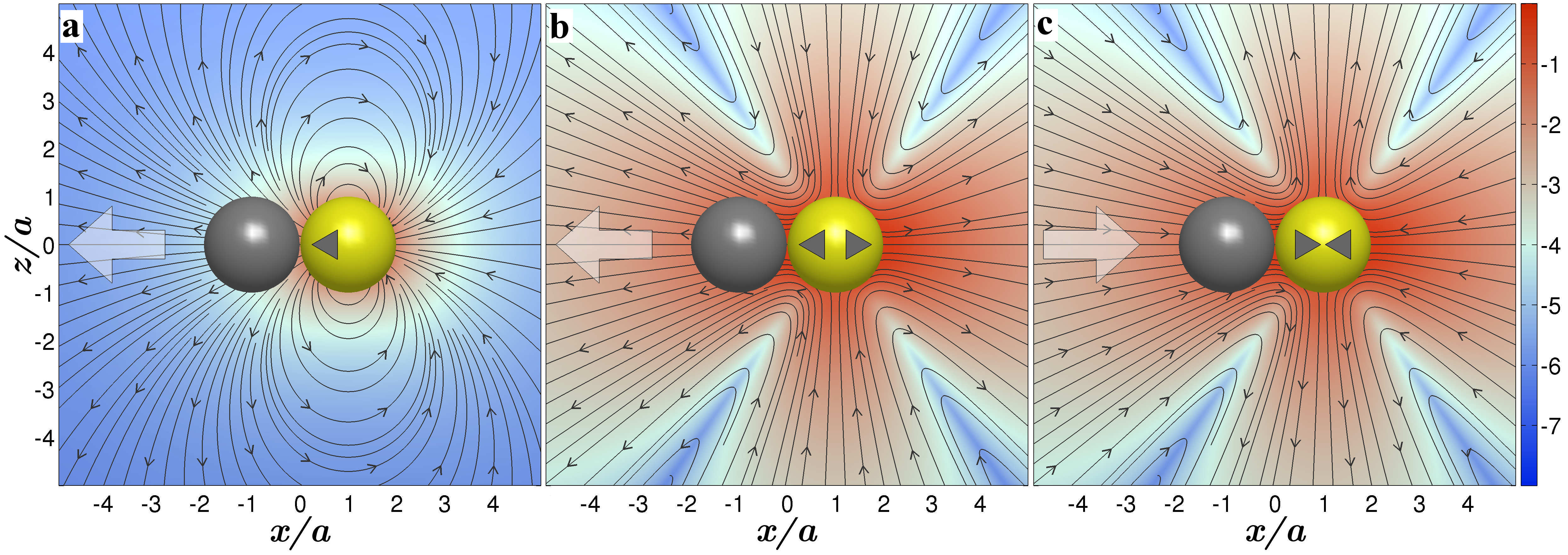
Figure 2: Motion of a passive colloid in the flow of an active colloid. The active is colloid is polar in panel (a), apolar and extensile in panel (b), and apolar and contractile in panel (c). The streamlines show active flow in the absence of the passive colloid. The background colour maps to the logarithm of the absolute value of the local flow field normalised by the global maximum. The large arrows show the direction of the force on the passive colloid exerted by the active flow.

III Diblock active filaments

In this section, we use the overdamped equations of motion of an active-passive mixture presented above to model a diblock active filament, consisting of chains of active and passive beads. In previous work jayaraman2012autonomous ; laskar2013hydrodynamic ; laskar2015brownian , we modelled an active slender body as a chain of active spheres. Here, we recall key elements of that work, while allowing some spheres to be passive.

A filament is obtained by connecting spheres by a potential $U$ that exerts forces ${\bf F}_{n}^{B}=-\bm{\nabla}_{n}U$ on the $n$-th sphere. The potential $U$ is the sum of connective, elastic, and self-avoiding steric potentials jayaraman2012autonomous ; laskar2013hydrodynamic . The relative importance of the $l\sigma$ mode of activity to the forces due to these potentials is quantified by dimensionless “activity” numbers,

$$\mathcal{A}{}^{l\sigma}=\frac{\left|\boldsymbol{\gamma}_{nm}^{(T,\,l\sigma)}\cdot\mathbf{V}_{m}^{(l\sigma)}\right|}{\left|\bm{\nabla}_{n}U\right|}$$ (7)

The filament dynamics is sensitive to the orientation of the principal axes $\mathbf{p}_{n}$ of the velocity coefficients $\mathbf{V}_{n}^{(l\sigma)}$ relative to the local Frenet-Serret frame attached to the filament, defined by the tangent $\mathbf{t}$, normal $\mathbf{n}$ and binormal $\mathbf{b}$ vectors. The most general parametrization of the relative orientation of the principal axis and the local frame is $\mathbf{p}_{n}=\,\alpha_{1}\mathbf{t}_{n}+\alpha_{2}\mathbf{n}_{n}+\alpha_{3}\mathbf{b}_{n}$. Torsional potentials can be introduced to penalize departures from this preferred orientation or constraint torques can be used to enforce the orientation exactly. In what follows, we choose the principal axis to be parallel to the local tangent and enforce this exactly through constraint torques. Since the orientation of the spheres is now subordinated to the local filament conformation, there is no independent angular degree of freedom. Therefore, the explicit form of the equation of motion of the diblock active filament is

$$\negthickspace\negthickspace\negthickspace\negthickspace\negthickspace\negthickspace\dot{\mathbf{R}}_{n} = \underbrace{\bm{\mu}_{nm}^{TT}\cdot\mathbf{F}_{m}^{B}+\bm{\mu}_{nm}^{TR}\cdot\mathbf{T}_{m}^{B}}_{\mathrm{Passive}}+\underbrace{\bm{\pi}_{nm}^{(T,\,l\sigma)}\cdot{\bf V}_{m}^{(l\sigma)}}_{\mathrm{Active}},$$ (8)

where it is understood that $\mathbf{V}_{n}^{(l\sigma)}=0$ for the $n=1,\ldots,M$ passive spheres, and that the torque $\mathbf{T}_{n}^{B}$ contains the constraints needed to maintain the principal axis parallel to the tangent. An estimate of the relative strengths of noise and activity shows that activity is between a $100$ to a $1000$ times more dominant than thermal fluctuations in many typical situations wang2013small ; singh2016traction . Accordingly, we neglect them for the remainder of this work.

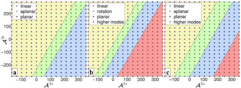
Figure 3: Stable states of actuation of a filament which is (a) free, (b) tethered, or (c) clamped, in the parameter space of $\mathcal{A}^{2s}$ and $\mathcal{A}^{3t}$, the dimensionless measures of apolar and polar activity. The net active force on the filament is guaranteed to be compressive in the fourth quadrant, $\mathcal{A}^{2s}>0$, $\mathcal{A}^{3t}<0$. Each dot represents one simulation and the background colours are a guide to the eye.

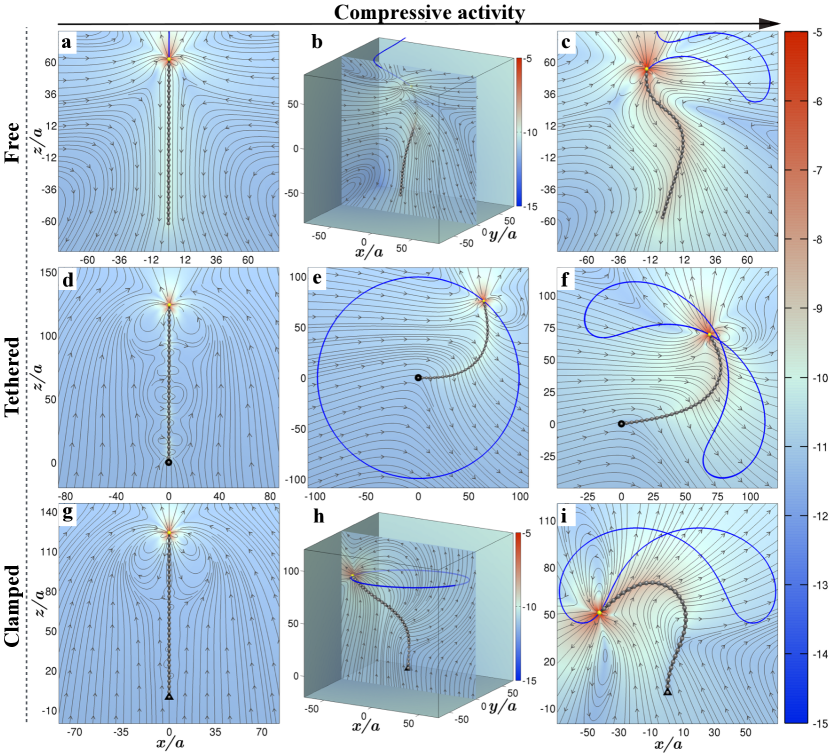
Figure 4: States of filament actuation for varying boundary conditions and activity. The top, middle, and bottom rows show a filament that is free, tethered and clamped respectively. The activity varies in the $\mathcal{A}^{2s}-\mathcal{A}^{3t}$ in such a manner that the compressive force due to the active colloid increases from left to right in each row. The precise values are tabulated in the Appendix. Streamlines show the net flow around the assembly, with the background coloured as in Fig. (2).

We now study a limiting case of these diblock active filaments where all but one sphere is passive. This provides the model of a passive filament actuated by an active colloid.

IV Passive filament - active colloid

We consider a diblock active filament in which the first $N-1$ spheres are passive and the $N$-th sphere is active, illustrated schematically in Fig. (1). The radii of the active and passive spheres are allowed to be different. The slip velocity of the active colloid is truncated at three terms, including the two leading polar terms and the leading apolar term,

$$\mathbf{v}(\bm{\rho}_{n}) =\dot{\mathbf{R}}_{n}-\underbrace{{\bf V}_{n}^{\mathcal{A}}+\tfrac{1}{15}{\bf V}_{n}^{(3t)}\cdot{\bf Y}^{(2)}}_{\mathrm{polar}}+\underbrace{{\bf V}_{n}^{(2s)}\cdot{\bf Y}^{(1)}}_{\mathrm{apolar}}$$ (9)

This model is sufficiently general to describe the far-field flow of a variety of polar and apolar active colloids ghose2014irreducible . We assume that the principal axes of the slip coefficients are parallel to the tangent vector, $\mathbf{t}_{N}$, at the terminus of the filament, so that

$${\bf V}_{N}^{(2s)}=as_{0}(\mathbf{t}_{N}\mathbf{t}_{N}-\frac{1}{3}\bm{\delta})$$ (10)

$${\bf V}_{N}^{\mathcal{A}}=-\frac{3}{5}{\bf V}_{N}^{(3t)}=-\frac{3a^{2}}{5}d_{0}\mathbf{t}_{N}.$$ (11)

Additionally, we neglect the subdominant contribution from the constant torques to the equations of motion. With these consideration, the explicit equation of motion for the filament and the active colloid are

$$\dot{\mathbf{R}}_{n}= -\frac{1}{6\pi\eta a}\bm{\nabla}_{n}U-\frac{1}{8\pi\eta}\sum_{m\neq n}\mathcal{F}^{0}\mathcal{F}^{0}\mathbf{G}\cdot\bm{\nabla}_{m}U+\frac{7a^{2}}{6}\mathcal{F}^{0}\mathcal{F}^{1}\bm{\nabla}_{N}\mathbf{G}\cdot{\bf V}_{N}^{(2s)}+\frac{a^{3}}{10}\nabla_{N}^{2}\mathbf{G}\cdot{\bf V}_{N}^{(3t)};\;n,m\in\mathrm{filament},$$ (12a)

$$\dot{\mathbf{R}}_{N}= -\frac{1}{6\pi\eta a}\bm{\nabla}_{N}U-\frac{1}{8\pi\eta}\sum_{m\neq N}\mathcal{F}^{0}\mathcal{F}^{0}\mathbf{G}\cdot\bm{\nabla}_{m}U-{\bf V}_{N}^{\mathcal{A}},\qquad\thinspace\thinspace\ \thinspace\thinspace\thinspace\thinspace\thinspace\thinspace\qquad\qquad\qquad\qquad\qquad\>\quad\qquad\mathrm{active\;colloid}.$$ (12b)

Here, $\mathcal{F}^{l}$ represents the correction due to the finite size of the spheres over the usual multipole expansion that implicitly assumes point particles. This Kirkwood-Riseman pair approximation is know to correct to $\mathcal{O}((a/b)^{3})$, where $b$ is the mean separation between the spheres of radius $a$ yoshizaki1980validity ; laskar2013hydrodynamic .

From the Eq. 7, it is clear that the two activity modes yield two activity numbers. In dimensionless units, theses numbers are $\mathcal{A}^{2s}$ and $\mathcal{A}^{3t}$ and expressed in terms of various system parameters as,

$$\mathcal{A}^{2s} =\frac{7\pi\eta a^{4}L^{2}s_{0}}{\kappa b^{2}}$$ (13)

$$\mathcal{A}^{3t} =\frac{18\pi\eta a^{3}L^{2}d_{0}}{5\kappa}$$ (14)

The principal role of the active sphere is to produce both a direct local force on the terminus of the filament and an indirect non-local force on the remaining parts of the filament mediated through the active contribution to the hydrodynamic flow. We now investigate the actuating dynamics of passive filament in the parameter space defined by the above two dimensionless groups.

Fig. (2) provides a good approximation to the local fluid flow near the terminus, with panel (a) corresponding to $\mathcal{A}^{3t}<0$, and panels (b) and (c) corresponding, respectively, to $\mathcal{A}^{2s}>0$ and $\mathcal{A}^{2s}<0$.

V Dynamics of actuation

As a prelude to presenting our main results, we first study the dynamics of and active and a passive colloid. The dynamics of the pair is presented in the figure 2. In panel (a), the active colloid is polar and motile with ${\bf V}_{N}^{\mathcal{A}}\neq 0$, while in panels (b) and (c) it is apolar and non-motile with ${\bf V}_{N}^{(2s)}\neq 0$. The choice of the sign of the principal value of $\mathbf{V}_{N}^{(2s)}$ corresponds to extensile (“pusher”) and contractile (“puller”) forms of apolar activity. The fluid-flow around the assembly is computed by using the Eq. 22 and the directions of movement of the pair for different cases are shown in white arrows. The direction and the speed of the pair critically depend on the relative position and orientation configuration of the colloids and the modes of activity. Surprisingly, we find that even a non-motile active colloid can function as a propulsion engine in the vicinity of a passive colloid. “Shakers” become “movers” in “passive” company. The significance of this observation for the colloid-filament assembly is explained below.

We turn now to our main numerical results. In Fig. (3) we show the state diagram, in the plane of the two dimensionless activity parameters, for the filament-colloid assembly. Positive (negative) values of $\mathcal{A}^{2s}$ corresponds to extensile (contractile) active flows while positive (negative) values of $\mathcal{A}^{3t}$ corresponds to self-propulsion outwards (towards) the assembly. The net effect of the active colloid is to produce a force which tends to extend (compress) the filament, when the parameters are in the second (fourth) quadrants of the $\mathcal{A}^{2s}-\mathcal{A}^{3t}$ plane. Thus, moving diagonally from the second to the fourth quadrant leads to an increasing active compression on the filament. In sequence, we observe a linear state, states in which the filament is non-linear but has a steady conformation, and finally states in which the filament conformation is a periodic or aperiodic function of time. The specific values of the activity numbers at which these states appear depend on the boundary condition (free, tethered, or clamped) but their sequence remains unaltered.

In Fig. (4) we show examples of the linear, non-linear steady and non-linear unsteady states of actuation, for each kind of boundary condition and for increasing values of net compressive activity, with the streamlines of fluid flow superimposed. The locus of the filament terminus is shown as a solid line for the non-linear states. The Supplementary Information contains animations of some of these states.

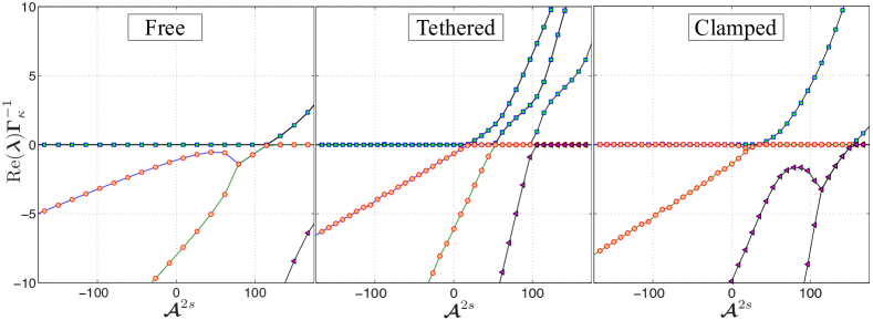
Figure 5: Variation of the real parts of the largest nonzero eigenvalues $\lambda$ of the stability matrix are plotted against dimensionless measure of apolar activity, $\mathcal{A}^{2s}$ for free, tethered and clamped boundary conditions. The transitions from the linear state to non-linear state proceeds via a Hopf bifurcation for the free and clamped cases and through a simple instability in the tethered case. $\Gamma_{\kappa}$ is the elastic relaxation rate jayaraman2012autonomous .

The nature of the dynamical transition from the linear state to the non-linear states can be quantified by a linear stability analysis. The variation of the largest non-zero eigenvalues of the stability matrix as a function of $\mathcal{A}^{2s}$ are shown in Fig. (5). The transition to non-linear state is through a Hopf bifurcation for free and clamped filaments but through a simple instability for the tethered for the filament. This is in contrast to a filament of hydrodynamically active dipoles in which the free and tethered states have simple instabilities while the clamped state has a Hopf bifurcation laskar2013hydrodynamic ; laskar2015brownian .

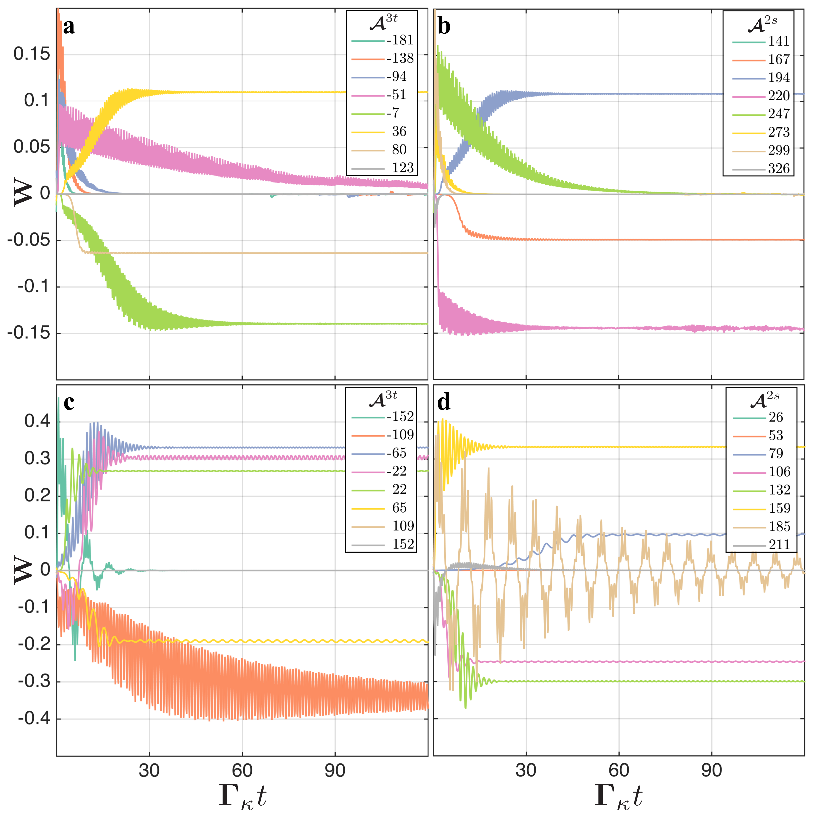
Figure 6: Time traces of the writhe of the assembly are presented with varying polar and apolar dimensionless numbers $\mathcal{A}^{3t}$ and $\mathcal{A}^{2s}$ for free (first row) and clamped assembly (second row). For all the subfigures, we see, that, for low activity both polar and apolar, the assembly relaxes back to linear conformation; in intermediate activity region, the assemblies, reach to steady states with constant or slightly oscillating writhe; at high activity, the assemblies, goes to a steady state with planar beating with zero writhe. Thus, using writhe along with the curvature, different regimes of steady states can clearly be demarcated.

In Fig. (6) we show the time series of the writhe,

$$W=\frac{1}{4\pi}\int_{C}\int_{C}d{\bf r}_{1}\times d{\bf r}_{2}\cdot\frac{{\bf r}_{1}-{\bf r}_{2}}{|{\bf r}_{1}-{\bf r}_{2}|^{3}}$$ (15)

a measure of the helicity of a three dimensional curve $C$, where, ${\bf r}_{1}$ and ${\bf r}_{2}$ are points on the curve. We use the method in klenin2000computation to estimate the integral from the discrete representation of the curve. The writhe and the curvature are used to demarcate the states in the Fig. (3). In earlier work, the convex hull of the filament conformation was used as an order parameter but we have found the writhe to be a more accurate and discriminatory measure of the stationary states.

We emphasise that the compressive forces that produce the rich dynamics have both a local contribution, communicated directly at the point of contact of the filament and the colloid and a non-local contribution that is mediated by the active flow produced by the colloid. While the local contribution acts directly on the bead to which the colloid is attached, the non-local contributions act on all the beads of the filament, though the strength decreases as the inverse of the square of the separation between bead and colloid. This non-local transmission of compressive forces is possible only when momentum conservation in the fluid is correctly accounted for. Hydrodynamic interactions, therefore, are of crucial importance in the dynamics uncovered here.

From the above analysis, it is now possible to choose states for specific biomimetic applications. The linear state of the free filament is the most efficient for transport and propulsion. Here, only a very small part of the active energy input is stored elastically in the filament as a small compression or extension. The balance is spent in transport. These, then, are the most efficient states for active transport. The non-linear states with steady conformations produce flow fields that co-rotate with the filament. These may be useful for producing low Reynolds number vortex fields in which large particles can be trapped or for stirring the medium. The non-linear states with unsteady conformations produce flow fields that promote efficient mixing of fluid. These may be used as components of artificial ciliary carpets that can mix and transport fluid along channels. It is conceivable that the filament-colloid assembly will find other imaginative uses in biomimetic applications singh2015nano ; guix2014nano ; garcia2013functionalized .

VI Discussion

While the actuation mechanism presented here is undoubtedly important in biomimetic applications it also has a connection to the study of “follower” forces in the mechanics of beams. These are forces that are always directed inwards along the local tangent at the end of the beam. The analysis of the instabilities of such a beam involves non-conservative forces for which the classical method of Euler is inapplicable bolotin1969effects . It is has been difficult to experimentally realize such beams and they remain a controversial topic in the theory of elastic stability elishakoff2005controversy . Our design points to a simple experimental realization of a slender elastic body driven by a “follower” force exerted by the active colloid. In addition, it provides yet another interesting angle for theoretical study, that is, the role of dissipation in elastic instabilities driven by non-conservative forces. We suggest these are interesting fields of enquiry in the growing literature on active filaments chelakkot2014flagellar ; jiang2014hydrodynamic ; ghosh2014dynamics ; jiang2014motion ; isele2015self ; winkler2016dynamics ; isele2016dynamics .

In this contribution, we have demonstrated that an elastic passive filament can be actuated without any external field by attaching an active colloid at its terminus. Though we have developed a theory considering Brownian motion, their contribution has been ignored in the present analysis. Here we conclude by pointing that the interplay between activity and Brownian motion has many interesting consequences that remain to be explored.

Appendix A Hydrodynamic tensors and fluid flow

The mobility and the propulsion tensors can be computed to any desired accuracy and order singh2016traction . The leading order forms in an unbounded medium, where $G_{ij}=\frac{\delta_{ij}}{r}+\frac{r_{i}r_{j}}{r^{3}}$ , are

$$8\pi\eta\bm{\mu}_{nm}^{TT} =\begin{cases}\frac{4}{3a}\bm{\delta}&\qquad\qquad\negthickspace m=n\\ \mathcal{F}^{0}\mathcal{F}^{0}\mathbf{G}(\mathbf{R}_{n},\mathbf{R}_{m})&\qquad\qquad\negthickspace m\neq n\end{cases}$$ (16)

$$8\pi\eta\bm{\mu}_{nm}^{TR} =\begin{cases}0&\qquad\quad\negthickspace m=n\\ \frac{1}{2}\bm{\nabla}_{m}\times\mathbf{G}(\mathbf{R}_{n},\mathbf{R}_{m})&\qquad\quad\negthickspace m\neq n\end{cases}$$ (17)

$$8\pi\eta\bm{\mu}_{nm}^{RT} =\begin{cases}0&\qquad\quad\negthickspace m=n\\ \frac{1}{2}\bm{\nabla}_{n}\times\mathbf{G}(\mathbf{R}_{n},\mathbf{R}_{m})&\qquad\quad\negthickspace m\neq n\end{cases}$$ (18)

$$8\pi\eta\bm{\mu}_{nm}^{RR} =\begin{cases}\frac{1}{a}\bm{\delta}&\negthickspace m=n\\ \frac{1}{4}\bm{\nabla}_{n}\times\bm{\nabla}_{m}\times\mathbf{G}(\mathbf{R}_{n},\mathbf{R}_{m})&\negthickspace m\neq n\end{cases}$$ (19)

The diagonal parts of these matrices are one-body terms while the off-diagonal parts represent the hydrodynamic interactions. The diagonal parts are the familiar Stokes translational and rotational mobilities while the off-diagonal parts can be recognised as the Rotne-Prager-Yamakawa tensors rotne1969variational ; yamakawa1970transport and their generalizations to rotational motion. The Onsager symmetry of the mobility matrix is manifest in these expressions. Similarly, the propulsion matrices can also be computed singh2014many , which are

$$\bm{\pi}_{nm}^{(T,\,l)} =\begin{cases}\bm{\delta}&m=n,\,l\sigma=1s\\ 0&m=n,\,l\sigma\neq 1s\\ c_{l}\mathcal{F}^{0}\mathcal{F}^{(l-1)}\mathbf{\bm{\nabla}}_{m}^{(l-1)}\mathbf{G}(\mathbf{R}_{n},\mathbf{R}_{m})&m\neq n\end{cases}$$ (20)

$$\bm{\pi}_{nm}^{(R,\,l)} =\begin{cases}\frac{1}{a}\bm{\delta}&\quad\>m=n,\,l\sigma=2a\\ 0&\quad\>m=n,\,l\sigma\neq 2a\\ \dfrac{c_{l}}{2}\bm{\nabla}_{n}\times\mathbf{\bm{\nabla}}_{m}^{(l-1)}\mathbf{G}(\mathbf{R}_{n},\mathbf{R}_{m})&\quad\>m\neq n\end{cases}$$ (21)

The form of mobility and propulsion matrices, we have thus got for beads of radius $a$ by considering solution after the first iteration, can be computed through alternative way through the pair-wise superposition approximation, first introduced by Kirkwood and Riseman kirkwood1948intrinsic , in their contributions on the dynamics of a polymer.

The fluid flow exterior to the filament-colloid assembly, with the two-mode truncation for the slip, is

$$\mathbf{v}(\mathbf{r})=-\frac{1}{8\pi\eta}\sum_{m=1}^{N}\mathcal{F}^{0}\mathbf{G}\cdot\bm{\nabla}_{m}U +\overbrace{\frac{7a^{2}}{6}\mathcal{F}^{1}\bm{\nabla}_{N}\mathbf{G}\cdot{\bf V}_{N}^{(2s)}}^{\mathrm{active}}$$

$$+\frac{a^{3}}{10}\nabla_{N}^{2}\mathbf{G}\cdot{\bf V}_{N}^{(3t)}.$$ (22)

This expression is used to plot the streamlines in the Fig.(2) and Fig.(4).

Appendix B Simulation parameters

The parameters we choose for the simulation as follows: bond-length $b_{0}=4a$, bending rigidity $\kappa=0.1$, spring constant $k=1$, non-motile activity or stresslet strength $s_{0}=-0.5-0.5$ and motile activity or degenerate quadrupole strength $d_{0}=-0.005-0.005$. The number of beads in the filament is $N=32$. We simulate the system for several hundred passive relaxation times $\Gamma_{\kappa}^{-1}$ while computing the hydrodynamic tensors at each time step using the PyStokes library singh2014pystokes . The initial condition in all simulations is the linear state with small-amplitude random transverse perturbations.

	Linear	Rotation or Helical	Planar mode
Free	$\mathcal{A}^{2s}\simeq 70$	$\mathcal{A}^{2s}\simeq 175$	$\mathcal{A}^{2s}\simeq 245$
	$\mathcal{A}^{3t}\simeq 90$	$\mathcal{A}^{3t}\simeq 0$	$\mathcal{A}^{3t}\simeq-60$
Tethered	$\mathcal{A}^{2s}\simeq 0$	$\mathcal{A}^{2s}\simeq 70$	$\mathcal{A}^{2s}\simeq 140$
	$\mathcal{A}^{3t}\simeq 90$	$\mathcal{A}^{3t}\simeq 60$	$\mathcal{A}^{3t}\simeq-30$
Clamped	$\mathcal{A}^{2s}\simeq-35$	$\mathcal{A}^{2s}\simeq 135$	$\mathcal{A}^{2s}\simeq 210$
	$\mathcal{A}^{3t}\simeq 120$	$\mathcal{A}^{3t}\simeq 0$	$\mathcal{A}^{3t}\simeq-90$

Table 1: Activity numbers correspond to panels of 4.

References

- [1] Christopher Brennen and Howard Winet. Fluid mechanics of propulsion by cilia and flagella. Annual Review of Fluid Mechanics, 9(1):339–398, 1977.
- [2] RA Lyons, E Saridogan, and O Djahanbakhch. The reproductive significance of human fallopian tube cilia. Human reproduction update, 12(4):363–372, 2006.
- [3] Yehoshua Enuka, Israel Hanukoglu, Oded Edelheit, Hananya Vaknine, and Aaron Hanukoglu. Epithelial sodium channels (enac) are uniformly distributed on motile cilia in the oviduct and the respiratory airways. Histochemistry and cell biology, 137(3):339–353, 2012.
- [4] Ann E Tilley, Matthew S Walters, Renat Shaykhiev, and Ronald G Crystal. Cilia dysfunction in lung disease. Annual review of physiology, 77:379–406, 2014.
- [5] Jahir Orozco, Beatriz Jurado-Sanchez, Gregory Wagner, Wei Gao, Rafael Vazquez-Duhalt, Sirilak Sattayasamitsathit, Michael Galarnyk, Allan Cortes, David Saintillan, and Joseph Wang. Bubble-propelled micromotors for enhanced transport of passive tracers. Langmuir, 30(18):5082–5087, 2014.
- [6] Wei Gao and Joseph Wang. The environmental impact of micro/nanomachines: a review. Acs Nano, 8(4):3170–3180, 2014.
- [7] Beatriz Jurado-Sanchez, Sirilak Sattayasamitsathit, Wei Gao, Luis Santos, Yuri Fedorak, Virendra V Singh, Jahir Orozco, Michael Galarnyk, and Joseph Wang. Self-propelled activated carbon janus micromotors for efficient water purification. Small, 11(4):499–506, 2015.
- [8] Virendra V Singh and Joseph Wang. Nano/micromotors for security/defense applications. a review. Nanoscale, 7(46):19377–19389, 2015.
- [9] Jahir Orozco, Guoqing Pan, Sirilak Sattayasamitsathit, Michael Galarnyk, and Joseph Wang. Micromotors to capture and destroy anthrax simulant spores. Analyst, 140(5):1421–1427, 2015.
- [10] Wentao Duan, Wei Wang, Sambeeta Das, Vinita Yadav, Thomas E Mallouk, and Ayusman Sen. Synthetic nano-and micromachines in analytical chemistry: Sensing, migration, capture, delivery, and separation. Annual Review of Analytical Chemistry, 8:311–333, 2015.
- [11] Wei Wang, Wentao Duan, Suzanne Ahmed, Thomas E Mallouk, and Ayusman Sen. Small power: Autonomous nano-and micromotors propelled by self-generated gradients. Nano Today, 8(5):531–554, 2013.
- [12] Maria Guix, Carmen C Mayorga-Martinez, and Arben Merkoçi. Nano/micromotors in (bio) chemical science applications. Chemical reviews, 114(12):6285–6322, 2014.
- [13] Sébastien Camalet, Frank Jülicher, and Jacques Prost. Self-organized beating and swimming of internally driven filaments. Physical review letters, 82(7):1590, 1999.
- [14] R Golestanian, TB Liverpool, and A Ajdari. Designing phoretic micro-and nano-swimmers. New Journal of Physics, 9(5):126, 2007.
- [15] Hassan Masoud, Benjamin I Bingham, and Alexander Alexeev. Designing maneuverable micro-swimmers actuated by responsive gel. Soft Matter, 8(34):8944–8951, 2012.
- [16] Eric E Keaveny, Shawn W Walker, and Michael J Shelley. Optimization of chiral structures for microscale propulsion. Nano letters, 13(2):531–537, 2013.
- [17] Brian J Williams, Sandeep V Anand, Jagannathan Rajagopalan, and M Taher A Saif. A self-propelled biohybrid swimmer at low reynolds number. Nature communications, 5, 2014.
- [18] Jaap MJ den Toonder and Patrick R Onck. Microfluidic manipulation with artificial/bioinspired cilia. Trends in biotechnology, 31(2):85–91, 2013.
- [19] Rolf E Isele-Holder, Julia Jäger, Guglielmo Saggiorato, Jens Elgeti, and Gerhard Gompper. Dynamics of self-propelled filaments pushing a load. Soft Matter, 2016.
- [20] MC Marchetti, JF Joanny, S Ramaswamy, TB Liverpool, J Prost, Madan Rao, and R Aditi Simha. Hydrodynamics of soft active matter. Reviews of Modern Physics, 85(3):1143, 2013.
- [21] Abhrajit Laskar and R Adhikari. Brownian microhydrodynamics of active filaments. Soft matter, 11(47):9073–9085, 2015.
- [22] Masao Doi. The theory of polymer dynamics. Number 73. oxford university press, 1988.
- [23] BV Derjaguin, IE Dzyaloshinsky, MM Koptelova, and LP Pitayevsky. Molecular-surface forces in binary solutions. Discussions of the Faraday Society, 40:246–252, 1965.
- [24] John L Anderson. Colloid transport by interfacial forces. Annual review of fluid mechanics, 21(1):61–99, 1989.
- [25] JR Blake. A spherical envelope approach to ciliary propulsion. Journal of Fluid Mechanics, 46(01):199–208, 1971.
- [26] Somdeb Ghose and R Adhikari. Irreducible representations of oscillatory and swirling flows in active soft matter. Physical review letters, 112(11):118102, 2014.
- [27] Rajesh Singh, Somdeb Ghose, and R Adhikari. Many-body microhydrodynamics of colloidal particles with active boundary layers. Journal of Statistical Mechanics: Theory and Experiment, 2015, 2014.
- [28] Rajesh Singh and R Adhikari. Traction relations for active colloids and their application. arXiv preprint arXiv:1603.05735, 2016.
- [29] Gayathri Jayaraman, Sanoop Ramachandran, Somdeb Ghose, Abhrajit Laskar, M Saad Bhamla, PB Sunil Kumar, and R Adhikari. Autonomous motility of active filaments due to spontaneous flow-symmetry breaking. Physical review letters, 109(15):158302, 2012.
- [30] Abhrajit Laskar, Rajeev Singh, Somdeb Ghose, Gayathri Jayaraman, PB Sunil Kumar, and R Adhikari. Hydrodynamic instabilities provide a generic route to spontaneous biomimetic oscillations in chemomechanically active filaments. Scientific reports, 3, 2013.
- [31] Takenao Yoshizaki and Hiromi Yamakawa. Validity of the superposition approximation in an application of the modified oseen tensor to rigid polymers. The Journal of Chemical Physics, 73(1):578–582, 1980.
- [32] Konstantin Klenin and Jörg Langowski. Computation of writhe in modeling of supercoiled dna. Biopolymers, 54(5):307–317, 2000.
- [33] Victor Garcia-Gradilla, Jahir Orozco, Sirilak Sattayasamitsathit, Fernando Soto, Filiz Kuralay, Ashley Pourazary, Adlai Katzenberg, Wei Gao, Yufeng Shen, and Joseph Wang. Functionalized ultrasound-propelled magnetically guided nanomotors: Toward practical biomedical applications. ACS nano, 7(10):9232–9240, 2013.
- [34] VV Bolotin and NI Zhinzher. Effects of damping on stability of elastic systems subjected to nonconservative forces. International Journal of Solids and Structures, 5(9):965–989, 1969.
- [35] Isaac Elishakoff. Controversy associated with the so-called “follower forces”: critical overview. Applied Mechanics Reviews, 58(2):117–142, 2005.
- [36] Raghunath Chelakkot, Arvind Gopinath, L Mahadevan, and Michael F Hagan. Flagellar dynamics of a connected chain of active, polar, Brownian particles. Journal of The Royal Society Interface, 11(92):20130884, 2014.
- [37] Huijun Jiang and Zhonghuai Hou. Hydrodynamic interaction induced spontaneous rotation of coupled active filaments. Soft matter, 10(46):9248–9253, 2014.
- [38] A Ghosh and NS Gov. Dynamics of active semiflexible polymers. Biophysical journal, 107(5):1065–1073, 2014.
- [39] Huijun Jiang and Zhonghuai Hou. Motion transition of active filaments: rotation without hydrodynamic interactions. Soft Matter, 10(7):1012–1017, 2014.
- [40] Rolf E Isele-Holder, Jens Elgeti, and Gerhard Gompper. Self-propelled worm-like filaments: spontaneous spiral formation, structure, and dynamics. Soft matter, 11(36):7181–7190, 2015.
- [41] Roland G Winkler. Dynamics of flexible active brownian dumbbells in the absence and the presence of shear flow. Soft matter, 12(16):3737–3749, 2016.
- [42] Jens Rotne and Stephen Prager. Variational treatment of hydrodynamic interaction in polymers. The Journal of Chemical Physics, 50(11):4831–4837, 1969.
- [43] Hiromi Yamakawa. Transport properties of polymer chains in dilute solution: hydrodynamic interaction. The Journal of Chemical Physics, 53(1):436–443, 1970.
- [44] John G Kirkwood and Jacob Riseman. The intrinsic viscosities and diffusion constants of flexible macromolecules in solution. The Journal of Chemical Physics, 16(6):565–573, 1948.
- [45] Rajesh Singh, Abhrajit Laskar, and R. Adhikari. Pystokes: Hampi, 2014.