Effect of Nonlinear Energy Transport on Neoclassical Tearing Mode Stability in Tokamak Plasmas
 
Richard Fitzpatrick
Institute for Fusion Studies
Department of Physics
University of Texas at Austin
Austin, TX 78712
 

Abstract

An investigation is made into the effect of the reduction in anomalous perpendicular electron heat transport inside the separatrix of a magnetic island chain associated with a neoclassical tearing mode in a tokamak plasma, due to the flattening of the electron temperature profile in this region, on the overall stability of the mode. The onset of the neoclassical tearing mode is governed by the ratio of the divergences of the parallel and perpendicular electron heat fluxes in the vicinity of the island chain. By increasing the degree of transport reduction, the onset of the mode, as the divergence ratio is gradually increased, can be made more and more abrupt. Eventually, when the degree of transport reduction passes a certain critical value, the onset of the neoclassical tearing mode becomes discontinuous. In other words, when some critical value of the divergence ratio is reached, there is a sudden bifurcation to a branch of neoclassical tearing mode solutions. Moreover, once this bifurcation has been triggered, the divergence ratio must reduced by a substantial factor to trigger the inverse bifurcation.

I Introduction

Neoclassical tearing modes are large-scale magnetohydrodynamical instabilities that cause the axisymmetric, toroidally-nested, magnetic flux-surfaces of a tokamak plasma to reconnect to form helical magnetic island structures on low mode-number rational magnetic flux surfaces.wesson Island formation leads to a degradation of plasma energy confinement.chang Indeed, the confinement degradation associated with neoclassical tearing modes constitutes a major impediment to the development of effective operating scenarios in present-day and future tokamak experiments.sauter Neoclassical tearing modes are driven by the flattening of the temperature and density profiles within the magnetic separatrix of the associated island chain, leading to the suppression of the neoclassical bootstrap current in this region, which has a destabilizing effect on the mode.car The degree of flattening of a given profile (i.e., either the density, electron temperature, or ion temperature profile) within the island separatrix depends on the ratio of the associated perpendicular (to the magnetic field) and parallel transport coefficients.rf

The dominant contribution to the perpendicular transport in tokamak plasmas comes from small-scale drift-wave turbulence, driven by plasma density and temperature gradients.wesson The fact that the density and temperature profiles are flattened within the magnetic separatrix of a magnetic island chain implies a substantial reduction in the associated perpendicular transport coefficients in this region. Such a reduction has been observed in gyrokinetic simulations,sim1 ; sim2 ; sim3 ; sim4 as well as in experiments.ex1 ; ex2 ; ex3 ; ex4 ; ex5 A strong reduction in perpendicular transport within the magnetic separatrix calls into question the conventional analytic theory of neoclassical tearing modes in which the perpendicular transport coefficients are assumed to spatially uniform in the island region.rf

The aim of this paper is to investigate the effect of the reduction in perpendicular transport inside the separatrix of a neoclassical magnetic island chain, due to profile flattening in this region, on the overall stability of the mode. For the sake of simplicity, we shall only consider the influence of the flattening of the electron temperature profile on mode stability. However, the analysis contained in this paper could be generalized, in a fairly straightforward manner, to take into account the influence of the flattening of the ion temperature and density profiles.

II Preliminary Analysis

II.1 Fundamental Definitions

Consider a large aspect-ratio, low-$\beta$, circular cross-section, tokamak plasma equilibrium. Let us adopt a right-handed cylindrical coordinate system ($r$, $\theta$, $z$) whose symmetry axis ($r=0$) coincides with the magnetic axis of the plasma. The system is assumed to be periodic in the $z$-direction with period $2\pi\,R_{0}$, where $R_{0}$ is the simulated major plasma radius. It is helpful to define the simulated toroidal angle $\varphi=z/R_{0}$. The coordinate $r$ serves as a label for the unperturbed (by the tearing mode) magnetic flux-surfaces. Let the equilibrium toroidal magnetic field, $B_{z}$, and the equilibrium toroidal plasma current both run in the $+z$ direction.

Suppose that a neoclassical tearing mode generates a helical magnetic island chain, with $m_{\theta}$ poloidal periods, and $n_{\varphi}$ toroidal periods, that is embedded in the aforementioned plasma. The island chain is assumed to be radially localized in the vicinity of its associated rational surface, minor radius $r_{s}$, which is defined as the unperturbed magnetic flux-surface at which $q(r_{s})=m_{\theta}/n_{\varphi}$. Here, $q(r)$ is the safety-factor profile (which is assumed to be a monotonically increasing function of $r$). Let the full radial width of the island chain’s magnetic separatrix be $W$. In the following, it is assumed that $\epsilon_{s}\equiv r_{s}/R_{0}\ll 1$ and $W/r_{s}\ll 1$.

It is convenient to employ a frame of reference that co-rotates with the magnetic island chain. All fields are assumed to depend (spatially) only on the radial coordinate $r$ and the helical angle $\zeta=m_{\theta}\,\theta-n_{\varphi}\,\varphi$. Let $k_{\theta}=m_{\theta}/r_{s}$, $q_{s}=m_{\theta}/n_{\varphi}$, and $s_{s}=d\ln q/d\ln r|_{r_{s}}$. The magnetic shear length at the rational surface is defined $L_{s}=R_{0}\,q_{s}/s_{s}$. Moreover, the unperturbed (by the magnetic island) electron temperature gradient scale-length at the rational surface takes the form $L_{T}=-1/(d\ln T_{0}/dr)_{r_{s}}$, where $T_{0}(r)$ is the unperturbed electron temperature profile. In the following, it is assumed that $L_{T}>0$, as is generally the case in conventional tokamak plasmas.wesson

The helical magnetic flux is defined

$$\chi(x,\zeta)=-\frac{B_{z}}{R_{0}}\int_{0}^{x}\left(\frac{1}{q}-\frac{1}{q_{s}}\right)(r_{s}+x)\,dx+\delta\chi(x,\zeta),$$ (1)

where $x=r-r_{s}$, and the magnetic field perturbation associated with the tearing mode is written $\delta{\bf B}=\nabla\times(\delta\chi\,{\bf e}_{z})$. It is easily demonstrated that ${\bf B}\cdot\nabla\chi=0$, where ${\bf B}$ is the total magnetic field.ruth Hence, $\chi$ is a magnetic flux-surface label. It is helpful to introduce the normalized helical magnetic flux, $\psi=(L_{s}/B_{z}\,w^{\,2})\,\chi$, where $w=W/4$. The normalized flux in the vicinity of the rational surface is assumed to take the form ruth

$$\psi(X,\zeta)=\frac{1}{2}\,X^{\,2}+\cos\zeta,$$ (2)

where $X=x/w$. As is well-known, the contours of $\psi$ map out a symmetric (with respect to $X=0$), constant-$\psi$,fkr magnetic island chain whose O-points lie at $\zeta=\pi$, $X=0$, and $\psi=-1$, and whose X-points lie at $\zeta=0$, $2\pi$, $X=0$, and $\psi=+1$. The chain’s magnetic separatrix corresponds to $\psi=+1$, the region inside the separatrix to $-1\leq\psi<1$, and the region outside the separatrix to $\psi>1$. The full radial width of the separatrix (in $X$) is 4.

Finally, the electron temperature profile in the vicinity of the rational surface is written

$$T(X,\zeta)=T_{s}\left[1-\left(\frac{w}{L_{T}}\right)\delta T(X,\zeta)\right],$$ (3)

where $T_{s}=T_{0}(r_{s})$, and

$$\left.\delta T(X,\zeta)\right|_{\lim|X|\rightarrow\infty}=X.$$ (4)

Note that $\delta T(X,\zeta)$ is an odd function of $X$. In the following, it is assumed that $w/L_{T}\ll 1$.

II.2 Electron Energy Conservation Equation

The steady-state electron temperature profile in the vicinity of the island chain is governed by the following well-known electron energy conservation equation: brag ; rf

$$\left(\frac{W}{W_{c}}\right)^{4}\left[\left[\delta T,\psi\right],\psi\right]+\frac{\partial^{\,2}\delta T}{\partial X^{\,2}}=0,$$ (5)

where

$$[A,B]\equiv\frac{\partial A}{\partial X}\,\frac{\partial B}{\partial\zeta}-\frac{\partial A}{\partial\zeta}\,\frac{\partial B}{\partial X},$$ (6)

and

$$W_{c}=4\left(\frac{\kappa_{\perp}}{\kappa_{\parallel}}\right)^{1/4}\left(\frac{L_{s}}{k_{\theta}}\right)^{1/2}.$$ (7)

Here, $\kappa_{\perp}$ and $\kappa_{\parallel}$ are the perpendicular (to the magnetic field) and parallel electron thermal conductivities, respectively. The first term on the right-hand side of Eq. (5) represents the divergence of the parallel (to the magnetic field) electron heat flux, whereas the second term represents the divergence of the perpendicular electron heat flux. [In fact, because $[[\delta T,\psi],\psi]$ and $\partial^{\,2}\delta T/\partial X^{\,2}$ are both ${\cal O}(1)$ in our normalization scheme, the ratio of the divergences of the parallel and perpendicular heat fluxes is effectively measured by $(W/W_{c})^{4}$.] The quantity $W_{c}$ is the critical island width above which the former term dominates the latter, causing the temperature profile to flatten within the island separatrix.rf In writing Eq. (5), we have neglected any localized sources or sinks of heat in the island region. We have also assumed that $\kappa_{\perp}$ and $\kappa_{\parallel}$ are spatially uniform in the vicinity of the rational surface. The latter assumption is relaxed in Sect. III

II.3 Narrow-Island Limit

Consider the so-called narrow-island limit in which $W\ll W_{c}$.rf Let

$$Y=\left(\frac{w}{w_{c}}\right)X.$$ (8)

Equation (5) transforms to give

$$\frac{\partial^{\,2}\delta T}{\partial Y^{\,2}}+Y^{\,2}\,\frac{\partial^{\,2}\delta T}{\partial\zeta^{\,2}} =-\left(\frac{W}{W_{c}}\right)^{\,2}\left(\sin\zeta\,\frac{\partial\,\delta T}{\partial\zeta}+2\,Y\,\sin\zeta\,\frac{\partial^{\,2}\delta T}{\partial Y\,\partial\zeta}+Y\,\cos\zeta\,\frac{\partial\,\delta T}{\partial Y}\right)$$

$$\phantom{=}-\left(\frac{W}{W_{c}}\right)^{\,4}\sin^{2}\zeta\,\frac{\partial^{\,2}\delta T}{\partial Y^{\,2}}.$$ (9)

We can write

$$\delta T(Y,\zeta)=\left(\frac{W_{c}}{W}\right)Y+\left(\frac{W}{W_{c}}\right)T_{1}(Y,\zeta)+{\cal O}\left(\frac{W}{W_{c}}\right)^{3},$$ (10)

where

$$\frac{\partial^{\,2}T_{1}}{\partial Y^{\,2}}+Y^{\,2}\,\frac{\partial^{\,2}T_{1}}{\partial\zeta^{\,2}}=-Y\,\cos\zeta,$$ (11)

subject to the boundary conditions $T_{1}(0,\zeta)=0$, and $T_{1}\rightarrow 0$ as $|Y|\rightarrow\infty$. Note that the solution (10) automatically satisfies the boundary condition (4). It follows that

$$T_{1}(Y,\zeta)=\frac{\sqrt{2}}{4}\,f\left(\sqrt{2}\,Y\right)\,\cos\zeta,$$ (12)

where $f(p)$ is the well-behaved solution of

$$\frac{d^{\,2}f}{dp^{\,2}}-\frac{1}{4}\,p^{\,2}\,f=-p$$ (13)

that satisfies $f(0)=0$, and $f\rightarrow 0$ as $|p|\rightarrow\infty$. Note that $f(-p)=-f(p)$. Hence, in the narrow-island limit,rf

$$\delta T(X,\zeta)=X+\left(\frac{W}{W_{c}}\right)\frac{\sqrt{2}}{4}\,f\left(\sqrt{2}\,\frac{W}{W_{c}}X\right)\,\cos\zeta+{\cal O}\left(\frac{W}{W_{c}}\right)^{3}.$$ (14)

II.4 Wide-Island Limit

Consider the so-called wide-island limit in which $W\gg W_{c}$.rf We can write

$$\delta T(X,\zeta)=\bar{T}(\psi)+\left(\frac{W_{c}}{W}\right)^{\,4}\tilde{T}(\psi,\zeta),$$ (15)

where $\bar{T}$ and $\tilde{T}$ are both ${\cal O}(1)$, and

$$\langle\tilde{T}\rangle=0.$$ (16)

Here, $\langle\cdots\rangle$ is the so-called flux-surface average operator.ruth This operator is defined as follows:

$$\langle A\rangle=\int_{\zeta_{0}}^{2\pi-\zeta_{0}}\frac{A_{+}(\psi,\zeta)}{\sqrt{2\,(\psi-\cos\zeta)}}\,\frac{d\zeta}{2\pi}$$ (17)

for $-1\leq\psi\leq 1$, and

$$\langle A\rangle=\int_{0}^{2\pi}\,\frac{A(s,\psi,\zeta)}{\sqrt{2\,(\psi-\cos\zeta)}}\,\frac{d\zeta}{2\pi}$$ (18)

for $\psi>1$, where $s={\rm sgn}(X)$, $\zeta_{0}=\cos^{-1}({\mit\psi})$, and

$$A_{+}(\psi,\zeta)=\frac{1}{2}\left[A(+1,\psi,\zeta)+A(-1,\psi,\zeta)\right].$$ (19)

Note that $\langle[A,\psi]\rangle\equiv 0$ for all $A$.

Equations (5) and (15) can be combined to give

$$[[\tilde{T},\psi],\psi]+\left(\frac{W_{c}}{W}\right)^{4}\frac{\partial^{\,2}\tilde{T}}{\partial X^{\,2}}+\frac{\partial^{\,2}\bar{T}}{\partial X^{\,2}}=0.$$ (20)

The flux-surface average of the previous equation yields

$$\left\langle\frac{\partial^{\,2}\bar{T}}{\partial X^{\,2}}\right\rangle={\cal O}\left(\frac{W_{c}}{W}\right)^{4},$$ (21)

which implies that

$$\frac{d}{d\psi}\left(\langle X^{\,2}\rangle\,\frac{d\bar{T}}{d\psi}\right)\simeq 0.$$ (22)

The previous equation can be integrated to give

$$\bar{T}(\psi)=\left\{\begin{array}[]{ccc}0&\mbox{\hskip 28.45274pt}&-1\leq\psi\leq 1\\[2.15277pt] s\int_{1}^{\psi}\frac{d\psi^{\prime}}{\langle X^{\,2}\rangle(\psi^{\prime})}&&\psi>1\end{array}\right.,$$ (23)

which satisfies the boundary condition (4). Hence, in the wide-island limit,rf

$$\delta T(X,\zeta)=\bar{T}(\psi)+{\cal O}\left(\frac{W_{c}}{W}\right)^{\,4}.$$ (24)

II.5 Modified Rutherford Equation

The temporal evolution of the island width is governed by the so-called modified Rutherford equation, which takes the form ruth ; rf ; car

$$G_{1}\,\tau_{R}\,\frac{d}{dt}\!\left(\frac{W}{r_{s}}\right)={\mit\Delta}^{\prime}\,r_{s}+G_{2}\,\alpha_{b}\,\frac{L_{s}}{L_{T}}\,\frac{r_{s}}{W},$$ (25)

where

$$G_{1} =2\int_{-1}^{\infty}\frac{\langle\cos\zeta\rangle^{\,2}}{\langle 1\rangle}\,d\psi,$$ (26)

$$G_{2} =16\int_{-1}^{\infty}\left\langle\frac{\partial T}{\partial X}\right\rangle\frac{\langle\cos\zeta\rangle}{\langle 1\rangle}\,d\psi.$$ (27)

Here, $\tau_{R}=\mu_{0}\,r_{s}^{\,2}/\eta(r_{s})$ is the resistive evolution timescale at the rational surface, and $\eta(r)$ is the unperturbed plasma resistivity profile. Moreover, ${\mit\Delta}^{\prime}<0$ is the standard linear tearing stability index.fkr Finally, $\alpha_{b}=f_{s}\,(q_{s}/\epsilon_{s})\,\beta$, where $f_{s}=1.46\,\epsilon_{s}^{\,1/2}$ is the fraction of trapped electrons, $\beta=\mu_{0}\,n_{s}\,T_{s}/B_{z}^{\,2}$, and $n_{s}$ is the unperturbed electron number density at the rational surface. The second term on the right-hand side of Eq. (25) parameterizes the destabilizing influence of the perturbed bootstrap current.rf ; car Note that, in this paper, for the sake of simplicity, we have employed the so-called lowest-order asymptotic matching scheme described in Ref. rf1, . This accounts for the absence of higher-order island saturation terms in Eq. (25).

III Effect of Temperature Flattening

III.1 Introduction

In conventional tokamak plasmas, the dominant contribution to the perpendicular electron thermal conductivity, $\kappa_{\perp}$, comes from small-scale drift-wave turbulence driven by electron temperature gradients.wesson The fact that the electron temperature gradient is flattened within the magnetic separatrix of a sufficiently wide magnetic island chain implies a substantial reduction in the perpendicular electron thermal conductivity in this region. There is clear experimental evidence that this is indeed the case.ex2 ; ex3 ; ex5 In particular, Ref. ex5, reports a reduction in $\kappa_{\perp}$ at the O-point of the magnetic island chain associated with a typical neoclassical tearing mode by 1 to 2 orders of magnitude. Obviously, such a strong reduction in $\kappa_{\perp}$ within the magnetic separatrix calls into question the conventional analytic model of neoclassical tearing modes, described in Sect. II, in which $\kappa_{\perp}$ is assumed to spatially uniform in the vicinity of the rational surface.

III.2 Nonuniform Perpendicular Electron Conductivity Model

As a first attempt to model the reduction in $\kappa_{\perp}$ due to temperature flattening within the magnetic separatrix of a neoclassical island chain, let us write

$$\kappa_{\perp}=\left\{\begin{array}[]{ccc}\kappa_{\perp\,1}&\mbox{\hskip 28.45274pt}&-1\leq\psi\leq 1\\[2.15277pt] \kappa_{\perp\,0}&&\psi>1\end{array}\right.,$$ (28)

where $\kappa_{\perp\,1}$ and $\kappa_{\perp\,0}$ are spatial constants, with $\kappa_{\perp\,1}\leq\kappa_{\perp\,0}$. Since the mean temperature gradient outside the separatrix of a neoclassical magnetic island chain is similar in magnitude to the equilibrium temperature gradient [see Eq. (42)], it is reasonable to assume that $\kappa_{\perp\,0}$ is equal to the local (to the rational surface) perpendicular electron thermal conductivity in the absence of an island chain.

Let

$$W_{c\,0} =4\left(\frac{\kappa_{\perp\,0}}{\kappa_{\parallel}}\right)^{1/4}\left(\frac{L_{s}}{k_{\theta}}\right)^{1/2},$$ (29)

$$W_{c\,1} =4\left(\frac{\kappa_{\perp\,1}}{\kappa_{\parallel}}\right)^{1/4}\left(\frac{L_{s}}{k_{\theta}}\right)^{1/2},$$ (30)

be the critical island widths outside and inside the separatrix, respectively. Likewise, let

$$\xi_{0} =\left(\frac{W}{W_{c\,0}}\right)^{4},$$ (31)

$$\xi_{1} =\left(\frac{W}{W_{c\,1}}\right)^{4},$$ (32)

measure the ratios of the divergences of the parallel and perpendicular electron heat fluxes outside and inside the separatrix, respectively. Finally, let the parameter

$$\lambda=\frac{\kappa_{\perp\,1}}{\kappa_{\perp 0}}=\frac{\xi_{0}}{\xi_{1}}$$ (33)

measure the relative reduction of perpendicular electron heat transport within the island separatrix.

Let us adopt the following simple model:

$$\lambda={\rm e}^{-\xi_{1}}+\left(1-{\rm e}^{-\xi_{1}}\right)\delta,$$ (34)

where $0<\delta\leq 1$. According to this model, the degree of perpendicular transport reduction within the separatrix is controlled by the parameter $\xi_{1}$, which measures ratio of the divergences of the parallel and perpendicular electron heat fluxes inside the separatrix. (See Sects. II.3 and II.4.) If $\xi_{1}$ is much less than unity then there is no temperature flattening within the separatrix, which implies that $\lambda=1$ (i.e., there is no reduction in transport). On the other hand, if $\xi_{1}$ is much greater than unity then the temperature profile is completely flattened inside the separatrix, and the transport is reduced by some factor $\delta$ (say). The previous formula is designed to interpolate smoothly between these two extremes as $\xi_{1}$ varies.

Equations (33) and (34) can be combined to give

$$\xi_{0}=\lambda\,\ln\left(\frac{1-\delta}{\lambda-\delta}\right).$$ (35)

If follows that $\delta\leq\lambda\leq 1$, with $\xi_{0}=0$ when $\lambda=1$, and $\xi_{0}\rightarrow\infty$ as $\lambda\rightarrow\delta$. It is easily demonstrated that the function $\xi_{0}(\lambda)$ has a point of inflection when $\delta=\delta_{\rm crit}=1/(1+{\rm e}^{\,2})=0.1192$. This point corresponds to $\xi_{0}=4\,\delta_{\rm crit}=0.4768$ and $\lambda=2\,\delta_{\rm crit}=0.2384$.

Figure 1 shows the perpendicular electron transport reduction parameter, $\lambda$, plotted as a function of the ratio of the divergences of the parallel to perpendicular electron heat fluxes outside the island separatrix, $\xi_{0}$, for various values of the maximum transport reduction parameter, $\delta$. It can be seen that if $\delta>\delta_{\rm crit}$ then the $\xi_{0}$–$\lambda$ curves are such that $d\xi_{0}/d\lambda<0$ for $\delta\leq\lambda\leq 1$. This implies that $\lambda$ decreases smoothly and continuously as $\xi_{0}$ increases, and vice versa. We shall refer to these solutions as continuous solutions of Eq. (35). On the other hand, if $\delta<\delta_{\rm crit}$ then the $\xi_{0}$–$\lambda$ curves are such that $d\xi_{0}/d\lambda>0$ for some intermediate range of $\lambda$ values lying between $\delta$ and $1$.

As illustrated in Fig. 2, the fact that if $\delta<\delta_{\rm crit}$ then $d\xi_{0}/d\lambda>0$ for intermediate values of $\lambda$ implies that there are two separate branches of solutions to Eq. (35)—the first characterized by $d\xi_{0}/d\lambda<0$ and relatively large $\lambda$, and the second characterized by $d\xi_{0}/d\lambda<0$ and relatively small $\lambda$. We shall refer to the former solution branch as the large-temperature-gradient branch [because it is characterized by a relatively large value of $\lambda$, which, from Eq. (34), implies a relatively small value of $\xi_{1}$, which, from Eq. (41), implies a relatively large electron temperature gradient inside the separatrix], and the latter as the small-temperature-gradient branch [because it is characterized by a relatively small value of $\lambda$, which, from Eq. (34), implies a relatively large value of $\xi_{1}$, which, from Eq. (41), implies a relatively small electron temperature gradient inside the separatrix]. The two solution branches are separated by a dynamically inaccessible branch characterized by $d\xi_{0}/d\lambda>0$. We shall refer to this branch of solutions as the inaccessible branch. Referring to Fig. 2, as $\xi_{0}$ increases from zero, we start off on the large-temperature-gradient solution branch, and $\lambda$ decreases smoothly. However, when a critical value of $\xi_{0}$ is reached (at which $d\xi_{0}/d\lambda=0$) there is a bifurcation to the small-temperature-gradient solution branch. We shall refer to this bifurcation as the temperature-gradient-flattening bifurcation, because it is characterized by a sudden decrease in the transport ratio parameter, $\lambda$, which implies a sudden decrease in the electron temperature gradient within the island separatrix. Once on the small-temperature-gradient solution branch, the control parameter $\xi_{0}$ must be reduced significantly in order to trigger a bifurcation back to the large-temperature-gradient solution branch. We shall refer to this bifurcation as the temperature-gradient-restoring bifuration, because it is characterized by a sudden increase in the transport ratio parameter, $\lambda$, which implies a sudden increase in the electron temperature gradient within the island separatrix

Figure 3 shows the critical values of the control parameter $\xi_{0}$ below and above which a temperature-gradient-flattening and a temperature-gradient-restoring bifurcation, respectively, are triggered, plotted as a function of $\delta/\delta_{\rm crit}$.

Figure 4 shows the extents of the various solution branches (i.e., the continuous, large-temperature-gradient, small-temperature-gradient, and inaccessible branches) plotted in $\xi_{0}$–$\xi_{1}$ space. It is clear that the large-temperature-gradient solution branch is characterized by $\xi_{0}\ll 1$ and $\xi_{1}\stackrel{{{}_{\normalsize<}}}{{{}_{\normalsize\sim}}}1$. In other words, the region outside the island separatrix lies in the narrow-island limit, $W\ll W_{c\,0}$, whereas that inside the separatrix lies in the narrow/intermediate island limit, $W\stackrel{{{}_{\normalsize<}}}{{{}_{\normalsize\sim}}}W_{c\,1}$. [See Eqs. (31) and (32).] This implies weak to moderate flattening of the temperature gradient within the separatrix. On the other hand, the small-temperarture-gradient solution branch is characterized by $\xi_{0}\ll 1$ and $\xi_{1}\gg 1$. In other words, the region outside the island separatrix lies in the narrow-island limit, $W\ll W_{c\,0}$, whereas that inside the separatrix lies in the wide-island limit, $W\gg W_{c\,1}$. This implies strong flattening of the temperature gradient within the separatrix. Figure 4 suggests that bifurcated solutions of Eq. (35) occur because it is possible for the regions inside and outside the island separatrix to lie in opposite asymptotic limits (the two possible limits being the wide-island and the narrow-island limits). Obviously, this is not possible in the conventional model in which $\kappa_{\perp}$ is taken to be spatially uniform in the island region.

Finally, according to our simple model, the critical value of the maximum transport reduction parameter, $\delta$, below which bifurcated solutions of the electron energy transport equation occur is $0.1192$. As we have seen, there is experimental evidence for a transport reduction within the separatrix of a neoclassical island chain by between 1 and 2 orders of magnitude.ex5 According to our model, such a reduction would be large enough to generate bifurcated solutions.

III.3 Composite Island Temperature Profile Model

Let

$$\delta T_{\rm narrow}(X,\zeta,\xi)=X+\xi^{1/4}\,\frac{\sqrt{2}}{4}\,f\left(\sqrt{2}\,\xi^{1/4}\,X\right)\,\cos\zeta$$ (36)

be the island temperature profile in the narrow-island limit. [See Eq. (14).] Here, $\xi=(W/W_{c})^{\,4}$. Likewise, let

$$\delta T_{\rm wide}(X,\zeta)=\left\{\begin{array}[]{ccc}0&\mbox{\hskip 28.45274pt}&-1\leq\psi\leq 1\\[2.15277pt] s\int_{0}^{\psi}\frac{d\psi^{\prime}}{\langle X^{\,2}\rangle(\psi^{\prime})}&&\psi>1\end{array}\right..$$ (37)

be the island temperature profile in the wide-island limit. [See Eqs. (23) and (24).] Let us write

$$\delta T(X,\zeta)=\left\{\begin{array}[]{ccc}\delta T_{\rm inside}(X,\zeta)&\mbox{\hskip 28.45274pt}&-1\leq\psi\leq 1\\[2.15277pt] \delta T_{\rm outside}(X,\zeta)&&\psi>1\end{array}\right.,$$ (38)

where [cf., Eq. (34)]

$$\delta T_{\rm inside}(X,\zeta)={\rm e}^{-\xi_{1}}\,\delta T_{\rm narrow}(X,\zeta,\xi_{1})+(1-{\rm e}^{-\xi_{1}})\,\delta T_{\rm wide}(X,\zeta)$$ (39)

and

$$\delta T_{\rm outside}(X,\zeta)={\rm e}^{-\xi_{0}}\,\delta T_{\rm narrow}(X,\zeta,\xi_{0})+(1-{\rm e}^{-\xi_{0}})\,\delta T_{\rm wide}(X,\zeta).$$ (40)

It follows that

$$\frac{\partial\,\delta T_{\rm inside}}{\partial X} \simeq{\rm e}^{-\xi_{1}}\left[1+\frac{f^{\prime}(0)}{2}\,\xi_{1}^{\,1/2}\,\cos\zeta+{\cal O}(\xi_{1})\right],$$ (41)

$$\frac{\partial\,\delta T_{\rm outside}}{\partial X} \simeq{\rm e}^{-\xi_{0}}\left[1+\frac{f^{\prime}(0)}{2}\,\xi_{0}^{\,1/2}\,\cos\zeta+{\cal O}(\xi_{0})\right]+(1-{\rm e}^{-\xi_{0}})\,\frac{X}{\langle X^{\,2}\rangle}.$$ (42)

Here, $f^{\prime}(0)=1.1981$, as determined from the numerical solution of Eq. (13).

III.4 Evaluation of Integrals

According to Eqs. (26), (27), (41), and (42),

$$G_{1} =2\,(I_{2}+I_{3}),$$ (43)

$$G_{2} =16\,I_{1}\,({\rm e}^{-\xi_{0}}-{\rm e}^{-\xi_{1}})+8\,f^{\prime}(0)\,I_{2}\,\xi_{1}^{\,1/2}\,{\rm e}^{-\xi_{1}}+8\,f^{\prime}(0)\,I_{3}\,\xi_{0}^{\,1/2}\,{\rm e}^{-\xi_{0}}$$

$$\phantom{=}+16\,I_{4}\,(1-{\rm e}^{-\xi_{0}}),$$ (44)

where

$$I_{1} =-\int_{-1}^{1}\langle\cos\zeta\rangle\,d\psi,$$ (45)

$$I_{2} =\int_{-1}^{1}\frac{\langle\cos\zeta\rangle^{\,2}}{\langle 1\rangle}\,d\psi,$$ (46)

$$I_{3} =\int_{1}^{\infty}\frac{\langle\cos\zeta\rangle^{\,2}}{\langle 1\rangle}\,d\psi,$$ (47)

$$I_{4} =\int_{1}^{\infty}\frac{\langle\cos\zeta\rangle}{\langle X^{\,2}\rangle\,\langle 1\rangle}\,d\psi.$$ (48)

Here, use has been made of the easily proved result

$$\int_{-1}^{\infty}\langle\cos\zeta\rangle\,d\psi=0.$$ (49)

Let $\psi=2\,k^{\,2}-1$. It follows that $d\psi=4\,k\,dk$. In the region $0\leq k\leq 1$, we can write

$$\zeta =2\,\cos^{-1}(k\,\sin\vartheta),$$ (50)

$$X =2\,k\,\cos\vartheta,$$ (51)

$$\cos\zeta =1-2\,(1-k^{\,2}\,\sin^{2}\vartheta),$$ (52)

$$\langle A\rangle =\int_{-\pi/2}^{\pi/2}\frac{A(k,\vartheta)}{\sqrt{1-k^{\,2}\,\sin^{2}\vartheta}}\,\frac{d\vartheta}{2\pi}.$$ (53)

On the other hand, in the region $k>1$, we can write

$$\zeta =\pi-2\,\vartheta,$$ (54)

$$X =2\sqrt{k^{\,2}-\sin^{2}\vartheta},$$ (55)

$$\cos\zeta =2\,k^{\,2}-1-2\,(k^{\,2}-\sin^{2}\vartheta),$$ (56)

$$\langle A\rangle =\int_{-\pi/2}^{\pi/2}\frac{A(k,\vartheta)}{\sqrt{k^{\,2}-\sin^{2}\vartheta}}\,\frac{d\vartheta}{2\pi}.$$ (57)

Here, it is assumed that $A$ is an even function of $X$.

Let

$${\cal A}(k) =2\,k\,\langle 1\rangle,$$ (58)

$${\cal B}(k) =2\,k\,\langle\cos\zeta\rangle,$$ (59)

$${\cal C}(k) =\frac{\langle X^{\,2}\rangle}{2\,k}.$$ (60)

It follows from Eqs. (50)–(57) that in the region $0\leq k\leq 1$,

$${\cal A}(k) =\frac{2}{\pi}\,k\,K(k),$$ (61)

$${\cal B}(k) =\frac{2}{\pi}\,k\left[K(k)-2\,E(k)\right].$$ (62)

On the other hand, in the region $k>1$,

$${\cal A}(k) =\frac{2}{\pi}\,K(1/k),$$ (63)

$${\cal B}(k) =\frac{2}{\pi}\left[(2\,k^{\,2}-1)\,K(1/k)-2\,k^{\,2}\,E(1/k)\right],$$ (64)

$${\cal C}(k) =\frac{2}{\pi}\,E(1/k).$$ (65)

Here,

$$K(k) =\int_{0}^{\pi/2}(1-k^{\,2}\,\sin^{2}\vartheta)^{-1/2}\,d\vartheta,$$ (66)

$$E(k) =\int_{0}^{\pi/2}(1-k^{\,2}\,\sin^{2}\vartheta)^{1/2}\,d\vartheta$$ (67)

are complete elliptic integrals.elliptic Hence, according to Eqs. (45)–(48) and (58)–(60),

$$I_{1} =-2\int_{0}^{1}{\cal B}\,dk=0.4244,$$ (68)

$$I_{2} =2\int_{0}^{1}\frac{{\cal B}^{\,2}}{\cal A}\,dk=0.3527,$$ (69)

$$I_{3} =2\int_{1}^{\infty}\frac{{\cal B}^{\,2}}{\cal A}\,dk=0.0587,$$ (70)

$$I_{4} =2\int_{1}^{\infty}\frac{{\cal B}}{{\cal A}\,{\cal C}}\,dk=0.3838.$$ (71)

Thus, Eqs. (43) and (44) yield

$$G_{1} =0.8227,$$ (72)

$$G_{2} =6.791\,({\rm e}^{-\xi_{0}}-{\rm e}^{-\xi_{1}})+3.380\,\xi_{1}^{\,1/2}\,{\rm e}^{-\xi_{1}}+0.562\,\xi_{0}^{\,1/2}\,{\rm e}^{-\xi_{0}}+6.140\,(1-{\rm e}^{-\xi_{0}}),$$ (73)

respectively.

III.5 Destabilizing Effect of Perturbed Bootstrap Current

The dimensionless parameter $G_{2}$, appearing in the modified Rutherford equation, (25), measures the destabilizing influence of the perturbed bootstrap current. Figure 5 shows $G_{2}$ plotted as a function of the so-called neoclassical tearing mode control parameter,

$$\xi_{0}=\left(\frac{W}{W_{c\,0}}\right)^{4}=\left(\frac{W}{4}\right)^{4}\left(\frac{\kappa_{\parallel}}{\kappa_{\perp\,0}}\right)\left(\frac{k_{\theta}}{L_{s}}\right)^{2},$$ (74)

which measures the ratio of the divergences of the parallel to the perpendicular electron heat fluxes outside the island separatrix. [See Eqs. (29) and (31).] The curves shown in this figure are obtained from Eqs. (33), (35), and (73). Note that $\kappa_{\parallel}$ and $\kappa_{\perp\,0}$ are the local (to the rational surface) parallel and perpendicular electron thermal conductivities, respectively, in the absence of an island chain.

It can be seen, from Fig. 5, that if the maximum transport reduction parameter, $\delta$, is relatively close to unity (implying a relatively weak reduction in the perpendicular electron thermal conductivity inside the island separatrix when the electron temperature profile is completely flattened in this region) then the bootstrap destabilization parameter, $G_{2}$, increases monotonically with increasing $\xi_{0}$, taking the value $3.492\,\xi_{0}^{\,1/2}$ when $\xi_{0}\ll 1$, and approaching the value $6.140$ asymptotically as $\xi_{0}\rightarrow\infty$.rf [These two limits follow from Eq. (73), given that $\xi_{1}\simeq\xi_{0}$ when $\lambda\simeq 1$.]

According to Fig. 5, as $\delta$ decreases significantly below unity (implying an increasingly strong reduction in the perpendicular electron thermal conductivity inside the island separatrix when the electron temperature profile is completely flattened in this region) it remains the case that $G_{2}=3.492\,\xi_{0}^{\,1/2}$ when $\xi_{0}\ll 1$, and $G_{2}\rightarrow 6.140$ as $\xi_{0}\rightarrow\infty$. However, at intermediate values of $\xi_{0}$ [i.e., $\xi_{0}\sim{\cal O}(1)$], the rate of increase of $G_{2}$ with $\xi_{0}$ becomes increasingly steep. This result suggests that a substantial reduction in the perpendicular electron thermal conductivity inside the island separatrix, when the electron temperature profile is completely flattened in this region, causes the bootstrap destabilization term in the modified Rutherford equation, (25), to “switch on” much more rapidly as the neoclassical tearing mode control parameter, $\xi_{0}$, is increased, compared to the standard case in which there is no reduction in the conductivity.

Finally, it is apparent from Fig. 5 that if $\delta$ falls below the critical value $\delta_{\rm crit}=0.1192$ then the bootstrap destabilization parameter, $G_{2}$, becomes a multi-valued function of $\xi_{0}$ at intermediate values of $\xi_{0}$. As illustrated in Fig. 6, this behavior is due to the existence of separate branches of solutions of the electron energy conservation equation. (See Sect. III.2.) The large-temperature-gradient branch is characterized by relatively weak flattening of the electron temperature profile within the island separatrix, and a consequent relatively small value (i.e., significantly smaller than the asymptotic limit $6.140$) of the bootstrap destabilization parameter, $G_{2}$. On the other hand, the small-temperature-gradient branch is characterized by almost complete flattening of the electron temperature profile within the island separatrix. Consequently, the bootstrap destabilization parameter, $G_{2}$, takes a value close to the asymptotic limit $6.140$ on this solution branch. The large-temperature-gradient and small-temperature-gradient solution branches are separated by a dynamically inaccessible branch of solutions. Referring to Fig. 6, as the neoclassical tearing mode control parameter, $\xi_{0}$, increases from a value much less than unity, we start off on the large-temperature-gradient solution branch, and the bootstrap destabilization parameter, $G_{2}$, increases smoothly and monotonically from a small value. However, when a critical value of $\xi_{0}$ is reached, there is a gradient-flattening-bifurcation to the small-temperature-gradient solution branch. This bifurcation is accompanied by a sudden increase in $G_{2}$ to a value close to its asymptotic limit $6.140$. Once on the small-temperature-gradient solution branch, $\xi_{0}$ must be decreased by a significant amount before a gradient-restoring-bifurcation to the large-temperature-gradient solution branch is triggered. Moreover, the gradient-restoring-bifurcation is accompanied by a very large reduction in $G_{2}$.

III.6 Long Mean-Free-Path Effects

The parallel electron thermal conductivity takes the form brag

$$\kappa_{\parallel}\sim n_{e}\,v_{e}\,\lambda_{e}$$ (75)

in a collisional plasma, where $n_{e}$ is the electron number density, $v_{e}$ is the electron themal velocity, and $\lambda_{e}$ is the electron mean-free-path. However, in a conventional tokamak plasma the mean-free-path $\lambda_{e}$ typically exceeds the parallel (to the magnetic field) wavelength $\lambda_{\parallel}$ of low-mode-number helical perturbations. Under these circumstances, the simple-minded application of Eq. (75) yields unphysically large parallel heat fluxes. The parallel conductivity in the physically-relevant long-mean-free-path limit ($\lambda_{e}\ll\lambda_{\parallel}$) can be crudely estimated as rf ; gor

$$\kappa_{\parallel}\sim n_{e}\,v_{e}\,\lambda_{\parallel},$$ (76)

which is equivalent to replacing parallel conduction by parallel convection in the electron energy conservation equation, (5). For a magnetic island of full radial width $W$, the typical value of $\lambda_{\parallel}$ is $n_{\varphi}\,s_{s}\,w/R_{0}$. Hence, in the long-mean-free-path limit, the expression for the neoclassical tearing mode control parameter (74) is replaced by

$$\xi_{0}=\left(\frac{W}{4}\right)^{5}\left(\frac{\kappa_{\parallel}^{\prime}}{\kappa_{\perp\,0}}\right)\left(\frac{k_{\theta}}{L_{s}}\right)^{2},$$ (77)

where $\kappa_{\parallel}^{\prime}=n_{\varphi}\,n_{e}\,v_{e}\,s_{s}/R_{0}$, and $n_{e}$ and $v_{e}$ are evaluated at the rational surface.

IV Summary and Discussion

In this paper, we have investigated the effect of the reduction in anomalous perpendicular electron heat transport inside the separatrix of a magnetic island chain associated with a neoclassical tearing mode in a tokamak plasma, due to the flattening of the electron temperature profile in this region, on the overall stability of the mode. Our model (which is described in Sect. III) is fairly crude, in that the perpendicular electron thermal conductivity, $\kappa_{\perp}$, is simply assumed to take different spatially-uniform values in the regions inside and outside the separatrix. Moreover, when the temperature profile is completely flattened within the island separatrix, $\kappa_{\perp}$ in this region is assumed to be reduced by some factor $\delta$, where $0<\delta\leq 1$. The degree of temperature flattening inside the separatrix is ultimately controlled by a dimensionless parameter $\xi_{0}$ that measures the ratio of the divergences of the parallel and perpendicular electron heat fluxes in the vicinity of the island chain. Expressions for $\xi_{0}$ in the short-mean-free-path and the more physically-relevant long-mean-free-path limits are given in Eqs. (74) and (77), respectively. Finally, the destabilizing influence of the perturbed bootstrap current is parameterized in terms of a dimensionless quantity $G_{2}>0$ that appears in the modified Rutherford equation. [See Eqs. (25) and (27).] A large value of $G_{2}$ implies substantial destabilization, and vice versa.

In the standard case $\delta=1$ (in which there is no reduction in the perpendicular electron thermal conductivity inside the island separatrix when the electron temperature profile is completely flattened in this region), the bootstrap destabilization parameter $G_{2}$ increases smoothly and monotonically as the control parameter $\xi_{0}$ increases, from a value much less than unity when $\xi_{0}\ll 1$, to the asymptotic limit $6.140$ when $\xi_{0}\gg 1$.rf (See Section III.5.)

As $\delta$ decreases significantly below unity (implying an increasingly strong reduction in the perpendicular electron thermal conductivity inside the island separatrix when the electron temperature profile is completely flattened in this region), the small-$\xi_{0}$ and large-$\xi_{0}$ behaviors of the bootstrap destabilization parameter remain unchanged. However, at intermediate values of the control parameter $\xi_{0}$ [i.e., $\xi_{0}\sim{\cal O}(1)$], the rate of increase of $G_{2}$ with $\xi_{0}$ becomes increasingly steep. (See Fig. 5.) In other words, a substantial reduction in the perpendicular electron thermal conductivity inside the island separatrix, when the electron temperature profile is completely flattened in this region, causes the bootstrap destabilization parameter $G_{2}$ to “switch on” much more rapidly as the control parameter $\xi_{0}$ is increased, compared to the standard case in which $\delta=1$. (See Section III.5.)

Finally, if $\delta$ falls below the critical value $0.1192$ then the bootstrap destabilization parameter, $G_{2}$, becomes a multi-valued function of the control parameter $\xi_{0}$, at intermediate values of $\xi_{0}$. This behavior is due to the existence of separate branches of solutions of the electron energy conservation equation. (See Sect. III.2.) The large-temperature-gradient branch is characterized by relatively weak flattening of the electron temperature profile within the island separatrix, and a consequent relatively small value (i.e., significantly smaller than the asymptotic limit $6.140$) of the bootstrap destabilization parameter, $G_{2}$. On the other hand, the small-temperature-gradient branch is characterized by almost complete flattening of the electron temperature profile within the island separatrix. Consequently, the bootstrap destabilization parameter, $G_{2}$, takes a value close to the asymptotic limit $6.140$ on this solution branch. The large-temperature-gradient and small-temperature-gradient solution branches are separated by a dynamically inaccessible branch of solutions. As the control parameter, $\xi_{0}$, increases from a value much less than unity, the system starts off on the large-temperature-gradient solution branch, and the bootstrap destabilization parameter, $G_{2}$, increases smoothly and monotonically from a small value. However, when a critical value of $\xi_{0}$ is reached, there is a gradient-flattening-bifurcation to the small-temperature-gradient solution branch. (See Fig. 6.) This bifurcation is accompanied by a sudden increase in $G_{2}$ to a value close to its asymptotic limit $6.140$. Once on the small-temperature-gradient solution branch, $\xi_{0}$ must be decreased by a significant amount before a gradient-restoring-bifurcation to the large-temperature-gradient solution branch is triggered. Moreover, the gradient-restoring-bifurcation is accompanied by a very large reduction in $G_{2}$. (See Section III.5.)

The behavior described in the preceding paragraph points to the disturbing possibility that a neoclassical tearing mode in a tokamak plasma could become essentially self-sustaining. In other words, once the mode is triggered, and the electron temperature profile is flattened within the island separatrix, the consequent substantial reduction in the perpendicular thermal conductivity in this region reinforces the temperature flattening, making it very difficult to remove the mode from the plasma.

Figure 1: The perpendicular electron transport reduction parameter, $\lambda$, plotted as a function of the ratio of the divergences of the parallel to perpendicular electron heat fluxes outside the island separatrix, $\xi_{0}$. The solid, short-dashed, long-dashed, dot-short-dashed, and dotted curves correspond to $\delta=0.9$, $0.5$, $0.2$, $0.1192$, and $0.01$, respectively. Here, $\delta$ is the maximum transport reduction parameter. The thin dot-long-dashed curve shows the locus of points where $d\xi_{0}/d\lambda=0$ ($d\xi_{0}/d\lambda>0$ to the left of the curve, and vice versa).

Figure 2: The solid curve shows the perpendicular electron transport reduction parameter, $\lambda$, plotted as a function of the ratio of the divergences of the parallel to perpendicular electron heat fluxes outside the island separatrix, $\xi_{0}$, for $\delta=0.01$. Here, $\delta$ is the maximum transport reduction parameter. The dot-long-dashed curve shows the locus of points where $d\xi_{0}/d\lambda=0$ ($d\xi_{0}/d\lambda>0$ to the left of the curve, and vice versa). The various solution branches and bifurcations are labeled.

Figure 3: The upper curve shows the critical value of the ratio of the divergences of the parallel to perpendicular electron heat fluxes outside the island separatrix, $\xi_{0}$, below which a temperature-gradient-flattening bifurcation is triggered, plotted as a function of $\delta/\delta_{\rm crit}$. The lower curve shows the critical value of $\xi_{0}$ above which a temperature-gradient-restoring bifurcation is triggered, plotted as a function of $\delta/\delta_{\rm crit}$. Here, $\delta$ is the maximum transport reduction parameter, and $\delta_{\rm crit}=0.1192$ is the critical value of $\delta$ below which bifurcations occur.

Figure 4: The extents of the various solution branches of Eq. (35) plotted in $\xi_{0}$–$\xi_{1}$ space. Here, $\xi_{0}$ is the ratio of the divergences of the parallel to perpendicular electron heat fluxes outside the island separatrix, whereas $\xi_{1}$ is the same ratio inside the separatrix.

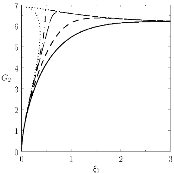
Figure 5: The bootstrap destabilization parameter, $G_{2}$, plotted as a function of the ratio of the divergences of the parallel to perpendicular electron heat fluxes outside the island separatrix, $\xi_{0}$. The solid, short-dashed, long-dashed, dot-short-dashed, and dotted curves correspond to $\delta=0.9$, $0.5$, $0.2$, $0.1192$, and $0.01$, respectively. Here, $\delta$ is the maximum transport reduction parameter.

Figure 6: The bootstrap destabilization parameter, $G_{2}$, plotted as a function of the ratio of the divergences of the parallel to perpendicular electron heat fluxes outside the island separatrix, $\xi_{0}$, for $\delta=0.01$. Here, $\delta$ is the maximum transport reduction parameter. The various solution branches and bifurcations are labeled.

References

- (1) J.A. Wesson, Tokamaks, 3rd Edition. (Oxford University Press, 2004).
- (2) Z. Chang, and J.D. Callen, Nucl. Fusion 30, 219 (1990).
- (3) O. Sauter, R.J. La Haye, Z. Chang, D.A. Gates, Y. Kamada, H. Zohm, et al., Phys. Plasmas 4, 1654 (1997).
- (4) R. Carrera, R.D. Hazeltine, and M. Kotschenreuther, Phys. Fluids 29, 899 (1986).
- (5) R. Fitzpatrick, Phys. Plasmas 2, 825, 1995.
- (6) W.A. Hornsby, A.G. Peeters, A.P. Snodin, F.J. Casson, Y. Camenon, G. Szepesi, M. Siccinio, and E. Poli, Phys. Plamas 17, 092301 (2010).
- (7) W.A. Hornsby, M. Siccinio, A.G. Peeters, E. Poli, A.P. Snodin, F.J. Casson, Y. Camenen, and G. Szepesi, Plasma Phys. Controlled Fusion 53, 054008 (2011).
- (8) P. Hill, F. Hariri, and M. Ottaviani, Phys. Plasmas 22, 042308 (2015).
- (9) O. Izacard, C. Holland, S.D. James, and D.P. Brennan, Phys. Plasmas 23, 022304 (2016).
- (10) C. Yu, D.L. Brower, S. Zhao, R.V. Bravenec, J. Chen, H. Lin, et al., Nucl. Fusion 32, 1545 (1992).
- (11) S. Inagaki, N. Tamura, K. Ida, Y. Nagayama, K. Kawahata, S. Sudo, et al., Phys. Rev. Lett. 92, 055002 (2004).
- (12) G.W. Spakman, G.D.M. Hogeweij, R.J.E. Jaspers, F.C. Schuller, E. Westerhof, J.E. Boom, et al., Nucl. Fusion 48, 065001 (2012).
- (13) K.J. Zhao, Y.J. Shi, S.H. Hahnand, P.H. Diamond, Y. Sun, J. Cheng, et al., Nucl. Fusion 55, 073022 (2015).
- (14) L. Bardóczi, T.L. Rhodes, T.A. Carter, N.A. Crocker, W.A. Peebles, and B.A. Grierson, Phys. Plasmas 23, 052507 (2016).
- (15) P.H. Rutherford, Phys. Fluids 16, 1903 (1973).
- (16) H.P. Furth, J. Killeen, and M.N. Rosenbluth, Phys. Fluids 6, 459 (1963).
- (17) S.I. Braginskii, in Reviews of Modern Physics. (Consultants Bureau, 1965). Vol. 1, p. 205.
- (18) R. Fitzpatrick, Phys. Plasmas 23, 122502 (2016).
- (19) M. Abramowitz, and I.A. Stegun (eds.), Handbook of Mathematical Functions with Formulas, Graphs, and Mathematical Tables. (Dover, 1965). Ch. 17.
- (20) N.N. Gorelenkov, R.V. Budny, Z. Chang, M.V. Gorelenkova, and L.E. Zakharov, Phys. Plasmas 3, 3379 (1996).