Epoch of Reionisation 21cm Forecasting From MCMC-Constrained Semi-Numerical Models

Abstract

The recent low value of Planck (2016) integrated optical depth to Thomson scattering suggests that the reionisation occurred fairly suddenly, disfavoring extended reionisation scenarios. This will have a significant impact on the 21cm power spectrum. Using a semi-numerical framework, we improve our model from Hassan et al. (2016) to include time-integrated ionisation and recombination effects, and find that this leads to more sudden reionisation. It also yields larger H ii bubbles which leads to an order of magnitude more 21cm power on large scales, while suppressing the small scale ionisation power. Local fluctuations in the neutral hydrogen density play the dominant role in boosting the 21cm power spectrum on large scales, while recombinations are subdominant. We use a Monte Carlo Markov Chain approach to constrain our model to observations of the star formation rate functions at $z=6,7,8$ from Bouwens et al. (2015), the Planck (2016) optical depth measurements, and the Becker & Bolton (2013) ionising emissivity data at $z\sim 5$. We then use this constrained model to perform 21cm forecasting for LOFAR, HERA, and SKA in order to determine how well such data can characterise the sources driving reionisation. We find that the 21cm power spectrum alone can somewhat constrain the halo mass dependence of ionising sources, the photon escape fraction and ionising amplitude, but combining the 21cm data with other current observations enables us to separately constrain all these parameters. Our framework illustrates how 21cm data can play a key role in understanding the sources and topology of reionisation as observations improve.

1 Introduction

The redshifted 21cm neutral hydrogen line from the Epoch of Reionisation (EoR) provides numerous astrophysical and cosmological information about the formation and evolution of the first stars and galaxies (Barkana & Loeb, 2001). Many ongoing and forthcoming experiments such as the Low Frequency Array (LOFAR), the Hydrogen Epoch of Reionisation Array (HERA), and the Square Kilometer Array (SKA-Low), are devoted to observing the dense neutral hydrogen gas that traces the cosmic web at redshifts beyond 7. While current experiments only yield upper limits to the measurements of the 21cm power spectrum, these future experiments are likely to provide a detection in the near future. It is thus important to develop robust and comprehensive theoretical models that can utilise such information, along with observations from other wavelengths and facilities, in order to optimally constrain the physical processes driving reionisation.

The recent low value of Planck (2016) integrated optical depth to Thomson scattering suggests that the EoR may have occurred more suddenly, and at much later times, than what was previously believed (Hinshaw et al., 2013). The low value of $\tau=0.058\pm 0.012$ prefers EoR models with late onset and shorter duration. This, in turn, is expected to have a significant impact on the expected 21cm signal and its evolution. Proper modeling of the sources and sinks of ionising photons during the EoR is required to accurately model the H ii bubbles and study their sizes and distributions. Doing so will enable us to connect the observed 21cm power spectrum with the physical properties of the sources and sinks of ionising photons during the EoR.

There are several major challenges to modeling the EoR and its redshifted 21cm signal, driven by the requirements for accurately modeling the power spectrum of H i on large scales. These requirements include: (i) large volumes ($\sim$ 500 Mpc) in order to capture the large scale H i fluctuations that will be detected in upcoming 21cm observations; (ii) high resolution that is sufficient to resolve the ionising sources and self-shielding systems on sub-kpc scales (Iliev et al., 2015); and (iii) accurate tracking of the ionising radiation and other feedback processes from the sub-kpc up to Mpc scales. For these reasons, self-consistently simulating the EoR represents an immense computational challenge that no current model has been able to fully meet.

Nonetheless, great progress has been made in simulating the EoR on both small and large scales. Hydrodynamic simulations that self-consistently incorporate radiative transfer (Gnedin 2000, 2014; Pawlik & Schaye 2008; Finlator & Davé 2009; Finlator et al. 2013; Katz et al. 2016) have sufficient resolution to model the sources of reionisation direction, and to propagate the emitted radiation through the intergalactic medium (IGM) with minimal physical assumptions. However, owing to computational limitations they are currently restricted to volumes smaller than $\sim 20$ Mpc in order to resolve all atomically-cooling halos. An alternative approach is to post-process simulated density fields with radiative transfer (Razoumov et al 2002; Mellema et al 2006; McQuinn et al 2007; Thomas et al 2009; Iliev et al. 2014; Bauer et al. 2015), which allows access to larger volumes but does not self-consistently account for thermal, ionisation, and chemical feedback effects on galaxy formation. Semi-analytical EoR models  (Mitra et al., 2011, 2013) are very successful in studying and constraining the globally averaged astrophysical quantities and parameters during EoR  (Mitra et al., 2012, 2015) based on current observations, but lack the dynamic range to study 21cm fluctuations. Finally, on the very largest scales, semi-numerical models (Mesinger & Furlanetto 2007; Zahn et al 2007; Choudhury et al 2009; Santos et al. 2010) based on quasi-linear density evolution with coarse modeling of the source population are able to access volumes sufficient to make 21cm predictions relevant to upcomgin observations, but must employ simple parameterised approximations for the source and sink populations. Nonetheless, such semi-numerical models, with appropriate tuning, can reproduce similar reionisaion histories as obtained by full radiative transfer simulations (Zahn et al 2011; Majumdar et al. 2014).

Semi-numerical models are most ideally suited for studying the large-scale ($\ga 1~{}Mpc$) 21cm power spectrum that will be measured with upcoming radio facilities, but they make many simplifying assumptions. In particular, they must assume parameterisations for the relationship between halo mass and ionising luminosity, and the relationship between the large-scale density field and the recombination rate that emerges from small-scale clumping. Also, current semi-numerical codes treat a single cell as either fully neutral or fully ionised, hence they must choose some condition to assign that cell as ionised. This third condition is an algorithmic choice, but the first two connect to physics, as they provide an opportunity to constrain astrophysical quantities associated with EoR sources and sinks based on 21cm and other EoR observations.

In Hassan et al. (2016), we focused on improving the physical parameterisations of the source and sink populations in the semi-numerical model SimFast21 by employing parameterised results from high-resolution radiative hydrodynamic simulations. This enabled greater physical realism of parameterised source and sink populations compared to previous approaches that had used a linear relationship between halo mass and luminosity, and did not include recombinations. To do this, we obtained parametrizations for the ionisation rate ${R_{\rm ion}}$ and recombination rate ${R_{\rm rec}}$ as functions of halo mass, overdensity, and redshift, extracted from high resolution radiative transfer hydrodynamic simulation (Finlator et al., 2015) (hearafter 6/256-RT) and larger-volume hydrodynamic simulation (Davé et al., 2013) (hereafter 32/512). We then implemented these parametrizations into SimFast21, and identified ionised regions where the ionisation rate exceeded the recombination rate. This more realistic modeling replaces the canonical efficiency parameter $\zeta$ approach in previous semi-numerical EoR modeling. In particular, we found that the ${R_{\rm ion}}$ scales super-linearly with halo mass (${R_{\rm ion}}\propto M^{1.4}_{h}$) in contrast to the typically assumed linear relationship between the efficiency parameter $\zeta$ and halo mass. We showed that using these new parametrizations (${R_{\rm ion}}$ and ${R_{\rm rec}}$) allows us to simultaneously match various EoR key observables with a relatively low escape fraction, independent of halo mass and redshift. We also found that the ${R_{\rm ion}}$ boosts the small scale 21cm power spectrum while ${R_{\rm rec}}$ suppresses the 21cm power on large scales during cosmic reionisations.

Hassan et al. (2016) thus improved upon the first two major uncertainties in semi-numerical models, namely the ionisation and recombinations. However, this work still assumed an ionisation condition based on the instantaneous balance between ionisations and recombinations – in other words, if there were instantaneously more ionisations than recombinations, that volume of space was considered fully ionised. However, this is not physically fully accurate, because the excess ionising photons in such regions still must ionise the neutral hydrogen atoms in that region. The instantaneous criterion thus does not account for partial ionisation of a given cell, thus it underestimates the total number of photons required. In the limiting case where reionisation proceeds quickly, this may not be a bad approximation, but ideally we aim to relax this instantaneous assumption. In essence, it is likely that our ionisations were too efficient, which can affect the topology and duration of the EoR along with our constraints on $f_{\mathrm{esc}}$.

In this paper, we improve upon our previous ionisation condition by tracking the actual number of neutral hydrogen atoms, ionising photons, and recombinations. This leads to a time dependent ionisation condition that is analogous to the well-known ionisation balance equation. With this, it turns out that reionisation occurs more suddenly, as preferred by the recent Planck (2016) constraints, but requires a higher escape fraction. We compare this to our previous Instantaneous EoR model Hassan et al. (2016) in terms of their H ii bubble sizes, EoR history, and 21cm power spectra.

Ideally, we would like to use the 21cm power spectra and other observations to provide constraints on the nature of the source population, in particular its relationship to the halo population. In Hassan et al. (2016), we manually constrained the relationship between ionising emissivity and halo mass versus observations, since we only had one free parameter, namely the escape fraction of ionising photons. This was because we had fixed the characteristics of the source population based on our radiative hydrodynamic simulations. Here we would like to relax this assumption, and determine how well we can constrain the source population characteristics directly from observations. To do this, we consider a generalised model with three free parameters: the escape photon fraction $\rm f_{\mathrm{esc}}$, the ionising emissivity amplitude $\rm A_{ion}$ (${R_{\rm ion}}$ amplitude), and the ionising emissivity-halo mass power-law index $\rm C_{ion}$. We note that $\rm C_{ion}$ can represent the power-law mass dependence of either the amplitude $\rm A_{ion}$ or the escape fraction $f_{\mathrm{esc}}$; in our current approach, these two quantities are degenerate. To constrain these parameters, we perform a Bayesian Monte Carlo Markov Chain (MCMC) search against current EoR observations. We then forecast how these constraints will be improved by upcoming 21cm observations from LOFAR, HERA, and SKA-Low. By considering all such observations, we determine how well we can constrain the EoR source population as characterised by our three free parameters.

This paper is organized as follows: In section 2, we introduce our previous Instantaneous EoR model and our new Time-integrated model. We study and compare these models’ impact on various EoR observables including the 21cm power spectrum in section3. In section 4, we create several EoR models to study their effects on the 21cm power spectrum. In section5, we calibrate the Time-integrated model to various EoR observations. We perform the 21cm forecasting in section6 and draw our concluding remarks in section 7.

Throughout this work, we adopt a $\Lambda$CDM cosmology in which $\Omega_{\rm M}=0.3$, $\Omega_{\rm\Lambda}=0.7$, $h\equiv H_{0}/(100\,\mathrm{km/s/Mpc})=0.7$, a primordial power spectrum index $n=0.96$, an amplitude of the mass fluctuations scaled to $\sigma_{8}=0.8$, and $\Omega_{b}=0.045$. We quote all results in comoving units, unless otherwise stated.

2 Simulations

We use a semi-numerical code SimFast21 (Santos et al. 2010), which we briefly review here. SimFast21 simulation begins by generating the density field from a Gaussian distribution using a Monte-Carlo approach. The generated density field will then be dynamically evolved from linear to non-linear regime by applying the Zel’Dovich (1970) approximation. The dark matter halos are generated using the well-known excursion-set formalism. In the standard SimFast21, the ionised regions are identified using the excursion-set formalism based on a constant efficiency parameter $\zeta$. In the original SimFast21 code, the ionisation condition compares the amount of collapsed dark matter halo $f_{coll}$ to the efficiency parameter $\zeta$ – any region will be flagged as ionised if:

$$f_{coll}\geq\zeta^{-1}.$$ (1)

The efficiency parameter $\zeta$ is a model free parameter which can be tuned to match some observations. This condition generates the ionisation field, which may be used along with the density field to obtain the 21cm brightness temperature. We refer the reader to Santos et al. (2010) for more details on this model and the code algorithm.

We now describe our two extensions to SimFast21. The first was presented in Hassan et al. (2016), which we review next, and incorporates the ionisation and recombination rate parameterisations taken from hydrodynamic simulations, but utilises an instantaneous ionisation condition. We then describe our further extension here in order to improve the ionisation condition by tracking the neutral fraction in a time-integrated manner. We will call this the “Instantaneous ionisation” and ”Time-integrated ionisation” models.

2.1 Instantaneous ionisation model

As described in Hassan et al. (2016), here we replace the efficiency parameter $\zeta$ with direct parameterisations of the ionisation rate ${R_{\rm ion}}$ and recombination rate ${R_{\rm rec}}$ as functions of halo mass $M_{h}$, overdensity $\Delta$, and redshift $z$, taken from our 6/256-RT and 32/512 simulations. Our best-fit non-linear ionisation rate ${R_{\rm ion}}$ parametrization takes the following form:

$$\mathrm{\frac{{R_{\rm ion}}}{M_{h}}=A_{ion}\,(1+z)^{D_{ion}}\,(M_{h}/B_{ion})^{C_{ion}}\,\exp\left(-(B_{ion}/M_{h})^{3.0}\right)},$$ (2)

where $\mathrm{A_{ion}}=1.08\times 10^{40}\;{\rm M}_{\odot}^{-1}$s^-1, $\mathrm{B_{ion}}=9.51\times 10^{7}\;{\rm M}_{\odot}$, $\mathrm{C_{ion}}=0.41$ and $\mathrm{D_{ion}}=2.28$. Meanwhile, we parameterise the recombination rate as:

$$\mathrm{\frac{{R_{\rm rec}}}{V}=A_{rec}(1+z)^{D_{rec}}\left[\frac{\left(\Delta/B_{rec}\right)^{C_{rec}}}{1+\left(\Delta/B_{rec}\right)^{C_{rec}}}\right]^{4}}\,,$$ (3)

where $\mathrm{A_{rec}}=9.85\times 10^{-24}$cm^-3s^-1, $\mathrm{B_{rec}}=1.76$, $\mathrm{C_{rec}}=0.82$, $\mathrm{D_{rec}}=5.07$.

Our ionisation condition is taken to be

$$\rm f_{\mathrm{esc}}R_{\mathrm{ion,V}}\geq R_{\mathrm{rec,V}}\,,$$ (4)

where

$$\rm R_{\mathrm{ion,V}}=\int_{dn}\int_{V}\frac{dn}{dM_{h}}{R_{\rm ion}}(M_{h},z)\,dM_{h}\,dV\,,$$

and

$$\rm R_{\mathrm{rec,V}}=\int_{V}\,{R_{\rm rec}}(\Delta,z)\,dV\,.$$

In above expressions, the $\rm f_{\mathrm{esc}}$ is the photon escape fraction, V is the spherical region volume specified by the excursion set-formalism, and n is the number density of halos. With these volume integrals, the $\rm R_{\mathrm{ion,V}}$ represents the total ionisation rate from all sources and $\rm R_{\mathrm{rec,V}}$ is the maximum recombination rate in that volume V. Cells in a given volume V satisfying this criterion (equation 4) are considered fully ionised, otherwise they are fully neutral.

Using this model, it has been shown in  Hassan et al. (2016) that one can match simultaneously several EoR key observables, such as  Planck (2015) optical depth,  Becker & Bolton (2013) ionising emissivity and  Fan et al (2006) filling factor measurement, by only a constant $\rm f_{\mathrm{esc}}=4-6\%$ independent of halo mass or redshift. We refer the reader to  Hassan et al. (2016) for more details about the model and these new parametrizations.

2.2 Time-integrated ionisation model

The model in  Hassan et al. (2016) (our Instantaneous EoR model) has several drawbacks. First, the ionisation condition, equation (4), is an instantaneous criterion which compares the escaped ionisation rate $f_{\mathrm{esc}}{R_{\rm ion}}$ with the recombination rate ${R_{\rm rec}}$, instead of comparing the actual numbers of ionising photons to that of recombinations. Second, the ionisation condition, equation (4), assumes maximum recombination rate ${R_{\rm rec}}$ from all cells/regions as if they were fully ionised.

To improve on these, we modify the ionisation condition to account for the evolving neutral hydrogen fraction, which allows us to account for the existing number of hydrogen atoms in each region as well as to compute the recombination based on the current ionised fraction. Hence we now employ a time dependent integral ionisation condition:

$$\rm f_{\mathrm{esc}}R_{\mathrm{ion,V}}\,\,dt\geq{I\!R}_{\mathrm{rec,V}}\,\,dt+N_{HI,V}\,,$$ (5)

where

$$\rm{I\!R}_{\mathrm{rec,V}}=\int_{V}x_{HII}\,{R_{\rm rec}}(\Delta,z)\,dV\,,$$

and

$$\rm N_{HI,V}=\int_{V}(1-x_{HII})\,N_{H}\,dV.$$

The $\rm x_{HII}$ and $\rm N_{H}$ here are the ionisation fraction and the total number of hydrogen in cells respectively. The dt represents the time duration between successive snapshots. We apply this new condition (equation 5) as follows: for each cell, we first compute the integrand of the LHS ($\rm f_{\mathrm{esc}}{R_{\rm ion}}dt$) and RHS ($\rm x_{HII}{R_{\rm rec}}dt+(1-x_{HII})NH$). We then apply the excursion set formalism to perform the spherical volume integral. Once again, the ionisation fraction is set to 1 (fully ionised) for cells in volumes that satisfy the ionisation condition (equation 5), otherwise they remain fully neutral with zero ionisation fraction.

The left hand side (LHS) of our new ionisation condition (equation 5) represents the actual number of escaped ionising photons being emitted in $dt$. The first term of the right hand side (RHS) of this condition is the actual number of recombinations occurring during $dt$ in regions with an ionisation fraction of $\rm x_{HII}$. This term then tracks the exact number of recombinations even from partially ionised regions with $\rm 0<x_{HII}<1$. This recombination term has no effect at early times of EoR when the universe is completely neutral, but becomes the dominant sink for ionising photons at late stages of the EoR (Sobacchi & Mesinger, 2014).

The second term of the RHS of equation (5) denotes the total number of neutral hydrogen in the simulation box. At early EoR stages, the escaped ionising photons (LHS) fights only with the neutral hydrogen term $\rm(1-x_{HII})N_{H}$. As the EoR proceeds, the neutral hydrogen term becomes less significant, and the recombinations start to play the leading role in forestalling reionisation. Hence this provides a more physically motivated ionisation condition, in a similar form to the standard ionisation balance equation.

The condition is clearly time-dependent, unlike the Instantaneous ionisation model for which the ionisation condition could be evaluated independently at each time-step. Thus our new scheme can be sensitive to the choice of the time-step $dt$ used to perform the integration. For instance, a larger $dt(dz)$ will result in more ionising photons and also more recombinations. This then leads to a wrong evolving ionisation balance. We have conducted convergence tests to determine that $\rm dz=0.125$ provides a numerically-converged answer (see Appendix A). Our new method thus requires higher computational cost to evolve the ionisation state forward in time. We will explore possible variations of the ionisation condition from equation  (5) in §4, to study their impact on the 21cm power spectrum.

It turns out, as we will show, that the instantaneous ionisation condition results in more extended reionisation history, while our new time-integrated condition yields more sudden reionisation. Next, we will investigate their differences in terms of the EoR history, topology, and the 21cm power spectrum.

3 Impact on EoR observables

We use the Full model from  Hassan et al. (2016) as our fiducial “Instantaneous” reionisation model. This model uses equation(4) to identify the ionised regions with $f_{\mathrm{esc}}=4\%$ in a large volume box of $L=300$ Mpc and a number of cells $N=560^{3}$. This model yields a maximum halo mass of $3.56\times 10^{12}M_{\odot}$ and a minimum halo mass of $1.28\times 10^{8}M_{\odot}$ at z=6. We have shown that this model matches various observations of the EoR including the Planck (2015) optical depth $\tau=0.066$. Using the same density field boxes and halo catalogues, we run our new Time-integrated reionisation model with parameters calibrated against various EoR key observations (see section 5), including the new Planck (2016) optical depth. The two models are tuned to different $\tau_{e}$ values, but we do our 21cm comparison at a given neutral fraction since it has been shown that the 21cm power spectrum shape is more sensitive to the neutral fraction (e.g. see Zahn et al 2007; Mesinger & Furlanetto 2007). We also verify this later by comparing the Instantaneous model power spectra at different redshifts for a fixed neutral fraction in figure 5 in §3.3. We thus begin by comparing the Instantaneous and Time-integrated models’ differences in terms of their global neutral fraction history.

3.1 EoR ionisation history

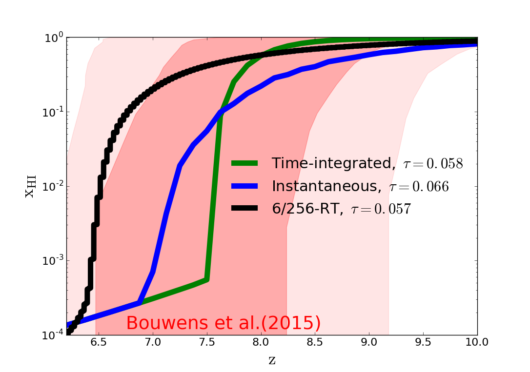
Figure 1: The volume-weighted average neutral fraction evolution as a function of redshift. The Time-integrated EoR model ($\tau=0.058$), the Instantaneous EoR model developed in Hassan et al. (2016) ($\tau=0.066$), and the 6/256-RT simulation ($\tau=0.057$) are represented by the green, blue, black lines, respectively. The shaded areas are several quasars and ly-$\alpha$ constraints as compiled by Bouwens et al. (2015). Its quite clear that all models are consistent with the observational constraints by Bouwens et al. (2015). Differences between models are explained in the text.

Figure 1 shows the global reionisation history produced by our two fiducial models, Instantaneous and Time-integrated, compared to the neutral fraction constraints obtained by Bouwens et al. (2015) via a compilation from various observables. We immediately see that the green line showing the new time-integrated ionisation condition shows a more sudden transition from fully ionised to fully neutral. Meanwhile, the blue line from our old instantaneous condition results in a more extended reionisation epoch. Nonetheless, in both cases, reionisation occurs in our two models within observational constraints (light-red shaded areas). It is perhaps worth noting that, unlike a few years ago when the canonical redshift for the end of reionisation was regarded as $z\sim 6$, current constraints from both observations and models favors the end of reionisation to occur at $z\sim 7$ or perhaps a bit higher.

This plot already shows that accounting for the neutral gas through comparing the number of neutral atoms and ionising photons (equation 5) versus comparing instantaneous rates (equation 4) has a significant impact on the reionisation history. The Time-integrated model is qualitatively more compatible with the picture that has been suggested by recent Planck (2016) constraints that favours sudden EoR scenarios. We emphasize the fact that if we tune the Time-integrated model optical depth to match the Instantaneous model optical depth ($\tau=0.066$, Planck 2015), the Time-integrated model will require higher $f_{\mathrm{esc}}$ and shift reionisation towards higher redshifts, but nevertheless the reionisation history shape will remain sudden as shown later in figure 9. We will come back to this point later in §5.2.2. However, when using the same parameters, the reionisation in the time-integrated model is delayed by $\Delta z\sim 0.8$ as compared with that in the instantaneous model.

From figure 1, we also see that both models Instantaneous and Time-integrated reionise the universe earlier than the 6/256-RT simulation. As discussed before in  Hassan et al. (2016), the small box size (6 h^-1 Mpc) of 6/256-RT does not capture the large scale fluctuations that give rise to the most massive halos that provide a significant fraction of reionising photons. Hence at a fixed optical depth, it is expected that the 6/256-RT might reionise the universe much later than the Time-integrated model due to the box size limitations.

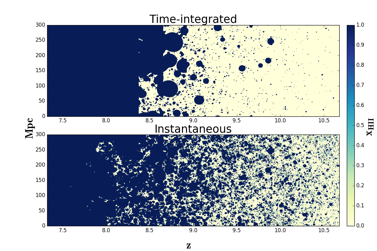
Figure 2: Evolving maps of the neutral fraction from the Instantaneous and Time-integrated models. Time-integrated EoR model produces large HII bubbles and reionises the universe very rapidly, indicating a sudden EoR scenario. Instantaneous EoR model yields small HII bubbles and reionises the universe very late, leading to an extended EoR scenario.

An informative way to examine these models is by viewing light cones, as shown in Figure 2. These have been constructed by projecting the ionisation state within the simulation volume along a specific line-of-sight, evolving with redshift. Figure 2 confirms that our previous model (the Full model of  Hassan et al. 2016) produces a more extended EoR scenario that corresponds to an early onset and a very late end with a duration of $\Delta z\sim 10$. Unlike the Instantaneous model, figure 2 also shows that our new model (equation 5) yields a sudden reionisation scenario where the EoR starts very late (once $\rm x_{HI}<1.0$ ) and ends (when $\rm x_{HI}$ drops below 10^-3) very quickly within a duration of $\Delta z\sim 4$. More strikingly, it also shows that the Time-integrated EoR model produces larger ionised bubbles while the Instantaneous model yields many ionised bubbles of smaller sizes. This can further be quantified by studying their differences in terms of the ionisation field power spectra.

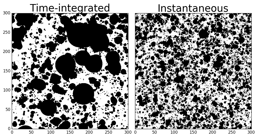
Figure 3: Slice of the ionistion box of a size $\rm 300\,\times\,300\,\times\,0.535\,Mpc^{3}$ from the Instantaneous and Time-integrated models and at $\rm x_{HI}\sim 0.5$. White and black represent neutral and ionised regions respectively. The self-shielded regions in ionised mediums are absent due to the binary structure of the excursion set formalism (assigning 1 to ionised and 0 to neutral cells in regions that satisfy the ionised condition) along with the large cell size of $\sim$ 0.5 Mpc.

3.2 EoR topology

It is useful to compare the models at a specific neutral fraction, since this best illustrates the difference in topology. Figure 3 compares our Instantaneous and Time-integrated models in terms of their ionisation maps when the EoR is half-way through, i.e. with a globally-averaged $\rm x_{HI}\sim 0.5$. These ionisation maps show the spatial distribution of the large and small ionised bubbles (black regions) over 300 Mpc scales. However, the excursion set-formalism with its binary structure (fully ionised or fully neutral), along with the large cell size of $\sim$ 0.5 Mpc, prevents these models’ maps to display the self-shielded regions in the ionised mediums as seen in figures 3 and 2. The presence of these self-shielded regions does not affect the 21cm power spectrum but rather lower the ionisation fraction at intermediate densities ($\Delta=5-10$) as previously shown (see figure (10) in Hassan et al. 2016). We also have shown in Hassan et al. (2016) that including the sub-clumping effect on scales below our cell size ($\sim$ 0.5 Mpc) have a minimal effect on the expected signal (see comparison between Full and NoSubClump models in Hassan et al. 2016 for more details).

From Figure 3, we see that the Instantaneous model produces many small H ii bubbles more uniformly distributed across the ionisation map. This shows that the EoR in the Instantaneous model proceeds from small scales, and the ionising photons are able to reionise locally everywhere. This is because the instantaneous ionisation rate can easily exceed the recombination rate (see equation (4)) on small scales when neglecting the local neutral hydrogen content.

In contrast, the Time-integrated model ionisation map shows very large H ii bubbles. This may be explained by interpreting the Time-integrated model ionisation condition (equation 5). As noted earlier, at high redshifts when the universe is neutral ($\rm x_{HII}\sim 0$), the recombination term can be neglected. In this case, the Time-integrated model only compares the escaped ionising photons with the total number of neutral hydrogen atoms. This condition dominates until the region becomes partially ionised. At that point, recombinations will start to occur because of the nonzero ionisation fraction $\rm x_{HII}$, but still this region is now less neutral, which will allow more rapid ionisation. However, different forms of ionisation condition yield very different HI fluctuations (see §4). In general, the sources and sinks are occurring within the regions that are densest and thus contain the most number of neutral hydrogen atoms. The high density causes the ionising photons to be ineffective at ionising local regions, until such time as significant ionisations happen, which then rapidly ionise the surrounding regions.

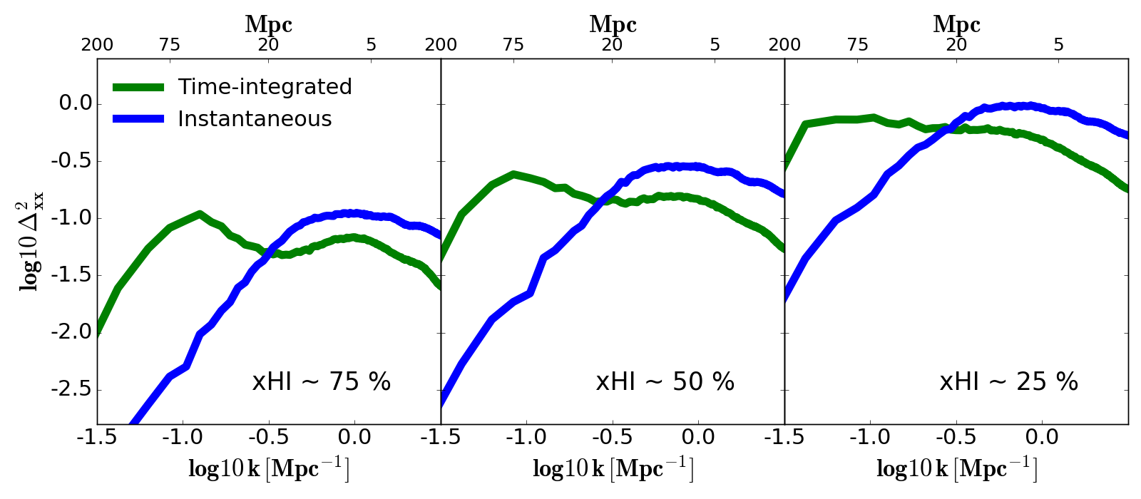
Figure 4: Ionization field power spectrum comparison between the Instantaneous (blue) and Time-integrated (green) models at different stages of reionisation ($\rm x_{HI}\,\sim\,25\%,\,50\%,\,75\%$.)

Figure 4 shows the ionisation field power spectra of our fiducial models at different stages of reionisation when the universe is 25%, 50% and 75% reionised. These neutral fractions correspond to z=8.0,8.75,9.5 and z= 7.75,8.0,8.25 as obtained by the Instantaneous and Time-integrated models respectively. This is computed as follows: $\mathrm{\Delta^{2}_{xx}\equiv k^{3}/|(2\pi^{2}\,V)<|x_{HII}|^{2}>/x^{2}_{HI}}$ (Hassan et al., 2016).

The Time-integrated model produces more power on large scales by 1-1.2 order of magnitude and less power on small scales by a factor of 2-3, at fixed ionisation fraction, as compared to the Instantaneous model. This is consistent with the qualitative impression from the ionisation maps in Figure 3. We further see that the large scale ionisation power spectrum, obtained by the Time-integrated EoR model, peaks at $\sim$ 75Mpc which corresponds to the characteristic size of the H ii bubbles as seen in the H ii maps in figure 3.

The difference particularly on large scales is substantial, which shows the importance of accounting for the existing neutral hydrogen content in the ionisation condition (i.e. the second term of equation (5)). Since the fluctuations in the ionisation field drive the 21cm brightness temperature, we expect to see similar differences in the 21cm power spectra, which we examine next.

3.3 The 21cm power spectrum

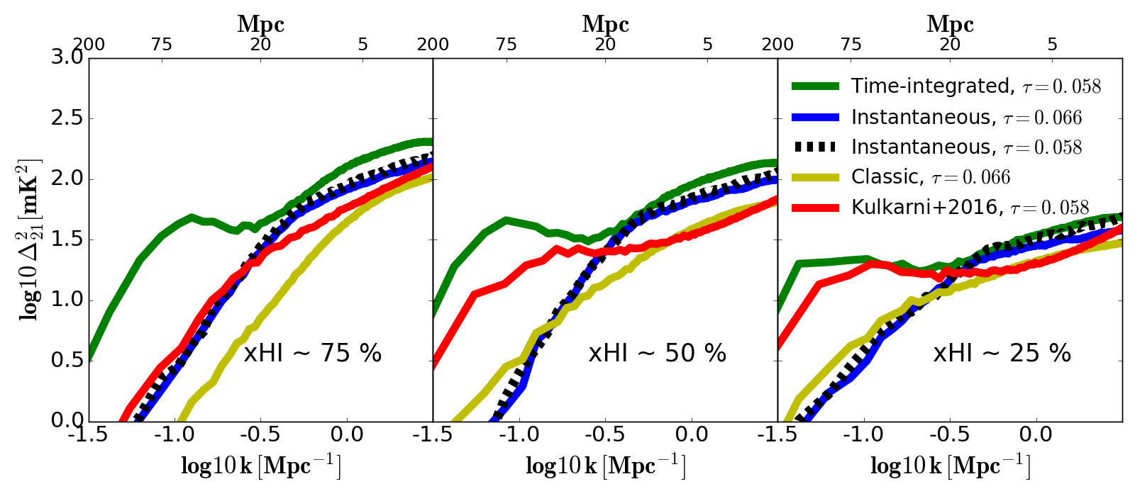
Figure 5: The 21cm power spectrum comparison between the Instantaneous (blue) and Time-integrated (green) models at different stages of reionisation ($\rm x_{HI}\,\sim\,25\%,\,50\%,\,75\%$). We compare our 21cm power spectra with the Very Late model (red) by similar semi-numerical method Kulkarni et al. (2016) that is calibrated to match Ly$\alpha$ and CMB data. Although our Time-integrated and Kulkarni et al. (2016) models correspond to different redshifts, but nevertheless the shape of the 21cm spectrum is similar, particularly at the intermediate and late stages of reionisations. We also show our Classic EoR model (yellow) from Hassan et al. (2016) which adopts the standard efficiency parameter approach similar to Kulkarni et al. (2016) model. Our Classic and Kulkarni et al. (2016) models produce similar power on small scales. The Instantaneous model, whether it is tuned to Planck (2016) $\tau$ (black dashed) or Planck (2015) $\tau$ (solid blue), always produces the exact 21cm power spectrum at fixed neutral fractions, regardless of the density field contribution from different redshifts. Models are tuned to the two recent Planck optical depth values as quoted in the legend.

Using the ionisation fields of these models, we now compute our EoR key observable which is the 21cm power spectrum. Assuming that the spin temperature is much higher than the CMB temperature, the 21cm brightness temperature takes the following form:

$$\delta T_{b}(\nu)=23\mathrm{x_{HI}}\Delta\left(\frac{\Omega_{b}h^{2}}{0.02}\right)\sqrt{\frac{1+z}{10}\frac{0.15}{\Omega_{m}h^{2}}}\left(\frac{H}{H+dv/dr}\right)\mathrm{mK},$$ (6)

where $dv/dr$ is the comoving gradient of the line of sight component of the comoving velocity. Using this equation, it is straightforward to create the 21cm brightness temperature boxes from which we compute the 21cm power spectrum as follows: $\mathrm{\Delta^{2}_{21}\equiv k^{3}/(2\pi^{2}\,V)<|\delta T_{b}(k)|^{2}_{k}>}$.

We first verify that the 21cm power spectrum is primarily sensitive to the global ionisation fraction, while the density field evolution is secondary. Note that the 21cm fluctuations traces those of the density field only at early times when the universe is almost neutral. Here we quote results for the Instantaneous model, but we expect that this is also valid for other models such as our Time-integrated model. We tune the Instantaneous model to Planck (2016) optical depth ($\tau=0.058$) which yields $\rm x_{HI}=0.75,0.54,0.277$ at $\rm z=8.75,8.00,7.25$ respectively. We then re-tune the model to the Planck (2015) optical depth ($\tau=0.066$) (similar to our previous Full model in Hassan et al. (2016)) to obtain $\rm x_{HI}=0.73,0.53,0.25$ at $\rm z=9.5,8.75,8.0$ respectively. We now compare their difference in the 21 power spectrum at these different redshifts for a fixed neutral fraction in figure 5. Comparing the solid blue line with black dashed line, we find the the Instantaneous model produces the exact 21cm power spectrum at a fixed neutral fraction, irrespective of the density field evolution at different redshifts. Hence we will compare different models at similar neutral fractions, not similar redshifts.

Figure 5 shows the 21cm power spectrum of the Instantaneous and Time-integrated models at neutral fractions of 25%, 50% and 75%. Mimicking the ionisation field power spectrum, the Time-integrated model produces more power on large scales by 1-1.2 order of magnitude at fixed ionisation fraction, as to that of the Instantaneous model. Likewise, the Time-integrated model also produces slightly more power on small scales by a factor of 1.2-1.5 as compared with the Instantaneous EoR model. This difference is less than when comparing the ionisation field power spectra, which comes from the contribution of the density field to the 21cm power spectrum – small regions with high local density (high recombinations) remain neutral, and hence they do not contribute much to the small-scale fluctuations in 21cm power.

We also compare our 21cm power spectra to a similar semi-numerical model by Kulkarni et al. (2016) that has been calibrated with Ly$\alpha$ and CMB data. The semi-numerical models by Kulkarni et al. (2016) adopts the standard efficiency parameter ($\zeta$) approach similar to our Classic EoR model (yellow in fig 5) from  Hassan et al. (2016). We choose to compare with the Very Late model in Kulkarni et al. (2016) (red in fig 5) that is tuned to match the Planck (2016) optical depth, consistent with the optical depth produced by our Time-integrated model. The ionisation histories of Kulkarni et al. (2016) and our Time-integrated model are very different even though they obtain $\sim 50\%$ neutral fraction at the same redshift. For instance, our Time-integrated model produces $\rm x_{HI}=0.77,0.57,0.25$ at z=8.25,8.0,7.75 whereas Kulkarni et al. (2016) model finds $\rm x_{HI}=0.84,0.59,0.42$ at z=10.0,8.0,7.0. Regardless of this difference in these models’ reionisation histories, their 21cm power spectra are generally similar. We find that both models produce a similar shape of the 21cm power spectrum particularly during the intermediate and final stages of reionisation. The minor difference in their amplitudes is due to using our ${R_{\rm ion}}$-${R_{\rm rec}}$ versus the standard $\zeta$ approach. This can be clearly seen when comparing our Classic EoR model with Kulkarni et al. (2016) model in figure 5. We see both models produce the same power on small scales while their difference on large scales might be from the difference in the density field and neutral fractions. This confirms our previous findings that using the non-linear ionisation power, via our ${R_{\rm ion}}$-${R_{\rm rec}}$ approach, boosts the 21cm power spectrum as compared to models adopting the standard efficiency parameter method (Classic and Kulkarni et al. (2016) models).

This shows that our Time-integrated model, that is calibrated to match various EoR key observables, produces similar 21cm power spectrum as obtained by other semi-numerical models that have been calibrated to match Ly$\alpha$ and CMB data. The future 21cm observations might be able to discriminate between these models’ power spectra.

In summary, we have compared the Instantaneous and Time-integrated models in terms of their EoR history, topology, and their 21cm power spectra. We have found that the Time-integrated model produces large HI bubbles while the Instantaneous model produces more small HI bubbles. The Time-integrated model yields a large scale 21cm/Ionization power spectrum that is higher by 1 order of magnitude as compared with the Instantaneous model. We have seen that the ionisation condition (equation 5) results in large H ii bubbles which boost the amount of power on large scales. The comparison presented here aims to summarize the differences found between our new (Time-integrated) and previous (Instantaneous) models. However, previous works by  Zahn et al (2011) and  Majumdar et al. (2014) have shown that semi-numerical simulations agree with radiative transfer simulations in terms of their ionization fields and 21cm power spectra. We leave for future work whether this new model matches radiative transfer simulations.

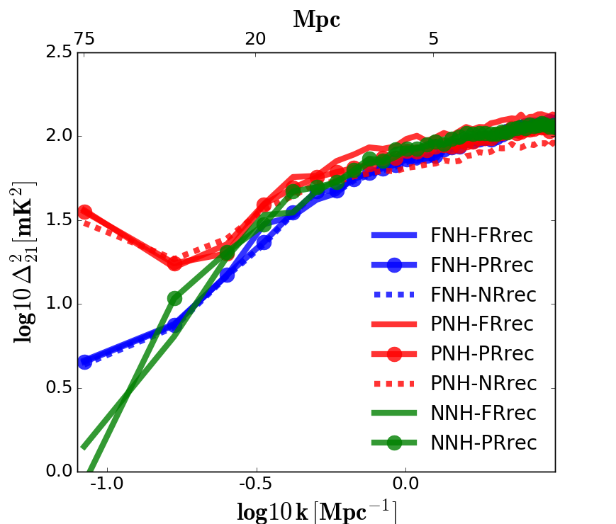
Figure 6: The 21cm power spectrum comparison for different physical assumptions at $\rm x_{HI}\,\sim\,50\%$. Different colors represent different ways to treat the local fluctuations in the neutral hydrogen density while different line styles corresponds to different recombinations terms, as explained by the legend and text. It is evident that the recombinations are subdominant in determining the large scale 21cm power spectrum. It is also shown models (red), that track the neutral fraction from partially ionised regions, yield a very high 21cm power spectrum on large scales.

4 Model assumption effects on the 21cm power spectrum

The large differences in the 21cm power spectrum (figure 5) between the Instantaneous and Time-integrated models show that the 21cm power spectrum is highly sensitive to the physical assumptions used. There are two main differences between these models: First, the ionisation condition now accounts for the number of hydrogen atoms, and second, the recombination is now done accounting for partial ionisation. We believe our new model is more physically-motivated and realistic, but we would like to understand exactly how these changes individually impact the 21cm power spectra.

We therefore consider the various possible combinations between ${R_{\rm rec}}$ and $\rm N_{H}$ to create several models with different ionisation condition. We also consider models neglecting recombination altogether to analyse the impact of recombinations as we did in Hassan et al. (2016), only with our new Time-integrated model.

More specifically, we keep the LHS of equation (5) (${R_{\rm ion}}$ term) same and vary the integrand of RHS integrals, namely $\rm{I\!R}_{\mathrm{rec,V}}$ and $\rm N_{HI,V}$, to create the following models:

• Full-NH-Full-Rrec (FNH-FRrec): $\rm{R_{\rm rec}}\,+N_{H}$.

• Full-NH-Partial-Rrec (FNH-PRrec): $\rm x_{HII}\,{R_{\rm rec}}\,+N_{H}$.

• Full-NH-No-Rrec (FNH-NRrec): $\rm N_{H}$.

• Partial-NH-Full-Rrec (PNH-FRrec): $\rm{R_{\rm rec}}\,+(1-x_{HII})\,N_{H}$.

• Partial-NH-Partial-Rrec (PNH-PRrec): $\rm x_{HII}\,{R_{\rm rec}}\,+(1-x_{HII})\,N_{H}$.

• Partial-NH-No-Rrec (PNH-NRrec): $\rm(1-x_{HII})\,N_{H}$.

• No-NH-Full-Rrec (NNH-FRrec): $\rm{R_{\rm rec}}\,$.

• No-NH-Partial-Rrec (NNH-PRrec): $\rm x_{HII}\,{R_{\rm rec}}\,$.

Model Class	Recombination term	Neutral Hydrogen term
Full-NH-Full-Rrec (FNH-FRrec)	$\rm{R_{\rm rec}}$	$\rm N_{H}$
Full-NH-Partial-Rrec (FNH-PRrec)	$\rm x_{HII}\,{R_{\rm rec}}$	$\rm N_{H}$
Full-NH-No-Rrec (FNH-NRrec)	0	$\rm N_{H}$
Partial-NH-Full-Rrec (PNH-FRrec)	$\rm{R_{\rm rec}}$	$\rm(1-x_{HII})\,N_{H}$
Partial-NH-Partial-Rrec (PNH-PRrec)	$\rm x_{HII}\,{R_{\rm rec}}$	$\rm(1-x_{HII})\,N_{H}$
Partial-NH-No-Rrec (PNH-NRrec)	0	$\rm(1-x_{HII})\,N_{H}$
No-NH-Full-Rrec (NNH-FRrec)	$\rm{R_{\rm rec}}$	0
No-NH-Partial-Rrec (NNH-PRrec)	$\rm x_{HII}\,{R_{\rm rec}}$	0

Table 1: Summary of models considered in section 4 for the 21cm power spectrum comparison in figure 6 from different physical assumnptions and treatment to the integrands of RHS integrals in the time-integrated ionisation condition, equation (5).

The Time-integrated model is represented here by ionisation condition of PNH-PRrec whereas the Instantaneous model uses that of NNH-FRrec. The others are variants on these as summarized in Table 1. To illustrate the differences in the 21cm power spectrum, we use the same density field and halo catalogues generated within a simulation run of a box size 75 Mpc and N = 140³. We have shown previously (Figure 8 in Hassan et al. 2016) that the numerical volume convergence of our simulated 21cm power spectrum is excellent at all redshifts down to a box size of 75 Mpc, hence, we expect the same 21cm power spectrum for larger simulation volumes. The reionisation history produced by these models vary, so as before we choose to make our 21cm power spectrum comparison at a fixed neutral fraction.

Figure 6 shows the 21cm power spectrum produced by different models at 50% neutral fraction as explained above. First, we see that all these variants result in virtually the same 21cm power spectrum on small scales. This reiterates our previous finding in  Hassan et al. (2016) that using a non-linear ionisation rate ${R_{\rm ion}}$ boosts the 21cm power spectrum by a similar amount regardless of whether one accounts for recombinations or not, and further shows that accounting for the neutral hydrogen atoms does not alter this conclusion.

More significant differences are evident at large scales for the 21cm power spectrum. Models starting with full $N_{H}$ (FNH-) produce 21cm power spectra with the same shape and amplitude on all scales (i.e. all the blue lines overlap), and likewise for models with partial or no $N_{H}$ (PNH- and NNH-). This demonstrates that recombinations are subdominant for determining the large-scale 21cm power spectrum. It is clear that the NH term plays a major role in boosting/suppressing the large scale 21cm power spectrum. This means that semi-numerical models must carefully account for the local number density of neutral hydrogen for a proper prediction of the expected signal.

From figure 6, we see the clear trend that models that do not account for the existing neutral hydrogen atoms (NNH- models such as the Instantaneous model) have lower 21cm power spectrum on large scales. Furthermore, models that use the total number of hydrogen atoms (FNH- models) at each time-step regardless of the ionisation fraction show 21cm power spectra that is slightly higher on large scales as compared to NNH- models. This is due to the presence of weak HI fluctuations by following only the density field ($\rm\bf N_{HI}\sim\Delta$). However, models, that use the ionisation history of cells to track the neutral hydrogen atoms from partially ionised regions (PNH- models such as the Time-integrated model), show a very high 21cm power spectrum on large scales as opposed to the NNH- and FNH- models. This comes from the fact that the the PNH- models account for a strong HI fluctuations by following the density field ($\rm\bf N_{HّّI}\sim\Delta$) and ionisation field ($\rm\bf N_{HّّّI}\sim x_{HII}$) both. This shows that, at given neutral fraction, the large scale 21cm power spectrum is highly influenced by the way in which we account for the fluctuations in the local neutral hydrogen density.

In the next section, we will discuss the calibration of the Time-integrated model against various EoR key observables and test how well the ongoing/upcoming 21cm observations will further constraints our free parameters.

5 Model calibration

We now focus on our favoured Time-integrated reionisation model, which includes all our new physics implementations. Previously, the parametrization of ${R_{\rm ion}}$ (equation 2) was obtained from our small-volume high-resolution radiative transfer hydrodynamic simulation (6/256-RT). However, the small volume of this simulation makes it subject to uncertainties since, as we saw in Figure 1, the ionisation history of this simulation is significantly delayed by its small volume. Here, we adopt a more general form for ${R_{\rm ion}}$, and determine whether existing EoR measurements can calibrate our source model, and thereby provide constraints on the nature of reionising sources.

To this end, we here consider a more generalized model with the following three free parameters:

• $f_{\mathrm{esc}}$ is the volume-averaged photon escape fraction.

• ${A_{\rm ion}}$ is the ionising emissivity amplitude, which scales the amount of ionising emissivity (${R_{\rm ion}}$) equally across the halo mass range at a given redshift.

• ${C_{\rm ion}}$ is ionising emissivity-halo mass power dependence, which quantifies the ${R_{\rm ion}}$-$M_{h}$ slope.

We will constrain these three parameters against various EoR observations and compare with the values found from fitting to the 6/256-RT simulation, using a Bayesian MCMC approach. We choose these parameters to explore since they are most closely related to the emission characteristics of the source population. We ignore $B_{\rm ion}$ which is related to how photoionisation suppresses low-mass galaxy growth, and $D_{\rm ion}$ because it is not physically obvious why ionisation rate of a given halo should have a strong redshift dependence. While it would be better to simply let all these parameters vary, even doing an MCMC over this 3-D space is already computationally challenging since it requires doing full runs for each sampling, and increasing the dimensionality quickly makes the computational requirements intractable.

Recall that the Time-integrated model identifies the ionised regions using a time dependent ionisation condition (equation 5), that tracks the exact recombinations and neutral hydrogen atoms by following the reionisation history. The reionisation history, in this model, is numerically well converged for $\Delta z\leq 0.125$. With these requirements, the model becomes more computationally expensive to run, but nevertheless, is feasible for independent large volume runs. However, sampling the full MCMC space requires at least $\sim\,10^{6}$ simulation realizations, which becomes infeasible. Hence we precompute a grid of models spanning the full prior space, and then do a trilinear interpolation to obtain the observables for any given parameter combination. This sacrifices some accuracy but makes the computation feasible.

We note that Greig & Mesinger (2015) developed an analysis pipeline, 21cmmc, that directly links their semi-numerical model 21CMFAST  (Mesinger et al., 2011) to a Bayesian routine cosmoHammar (Akeret et al., 2013) to constraining their free parameters. However, their ionisation condition did not include recombinations through the time integral method which they developed in Sobacchi & Mesinger (2014), and instead used a standard efficiency parameter ($\zeta$) approach. Along with lower resolution of $\sim\,$ 2 Mpc, these simplifications enabled them to run their semi-numerical model fully within an MCMC scheme.

5.1 Parameter estimations pipeline

We choose a cell size of 0.375 h^-1 Mpc and a box size $L=75$ Mpc, giving $N=140$ cells per side. We precompute a grid of $25\times 25\times 25$ runs outputting the predicted observables for our models, uniformly sampling our selected prior range for our parameters of ($f_{\mathrm{esc}},\,\rm log10(A_{ion}),\,C_{ion}$) = [(0,1),(37,44),(-1,2)]. This gives a total of 15,625 simulation independent realizations, which we interpolate inside the MCMC search process.

We have tested our parameter constraints using two different Bayesian inference tools Multinest (Feroz et al., 2009) and emcee (Foreman-Mackey et al., 2013). We have found the same parameter estimates using these two different codes, and hence, our presented parameters estimation here appear to be robust to variations in the algorithm used.

EoR Constraint	${\rm\bf f_{\mathrm{esc}}}$	${\rm\bf log10(A_{ion})}$	${\rm\bf C_{ion}}$
Bouwens et al. (2015) SFR all at z=8,7,6	0.51${}^{+0.33}_{-0.34}$	39.61${}^{+0.18}_{-0.16}$	0.45${}^{+0.08}_{-0.09}$
Planck (2016) optical depth $\tau$	0.46${}^{+0.36}_{-0.32}$	39.08${}^{+1.39}_{-1.44}$	0.28${}^{+0.76}_{-0.88}$
Becker & Bolton (2013) ionising emissivity $\bf\rm N_{ion}$ at z=4.75	0.51${}^{+0.34}_{-0.34}$	39.68${}^{+0.93}_{-1.36}$	-0.12${}^{+0.78}_{-0.62}$
ALL = SFR+$\tau$+$\rm N_{ion}$	0.25${}^{+0.26}_{-0.13}$	39.62${}^{+0.17}_{-0.18}$	0.44${}^{+0.09}_{-0.09}$
Values obtained from fitting to 6/256-RT	-	40.03	0.41

Table 2: Summary of our parameter estimations from individual and combined set of observations, as well as from matching to the 6/256-RT simulations.

We here present the results obtained by using the emcee python package. We use 100 random walkers initialised around the maximum likelihood. For each walker, we sample 10,000 chains from the likelihood after 500 initial burn-in chains to achieve convergence. This makes a total of 1,000,000 samples which is sufficient to explore the whole parameter space.

5.2 EoR key observables constraints

We constrain our three free parameters to the following observations:

1. The dust-corrected star formation rate density integrated down to $\rm M_{AB}=-17$ by Bouwens et al. (2015) at the following redshifts:

   • z $\sim$ 6: log10(SFR) [M_⊙ Mpc^-3 yr^-1] = -1.55 $\pm$ 0.06.

   • z $\sim$ 7: log10(SFR) [M_⊙ Mpc^-3 yr^-1] = -1.69 $\pm$ 0.06.

   • z $\sim$ 8: log10(SFR) [M_⊙ Mpc^-3 yr^-1] = -2.08 $\pm$ 0.07.

2. The Planck (2016) integrated optical depth to Thomson scattering: $\tau=0.058\pm 0.012$.

3. The Becker & Bolton (2013) ionising emissivity density measurements from Ly$\alpha$ data at $z=4.75$: $\rm\dot{N}ion$ [10⁵¹ photons s^-1 Mpc^-3] $=-0.014^{+0.454}_{-0.355}$.

We will first examine how our free parameters are constrained individually be each observation, and then we will examine the combined constraints.

5.2.1 The Bouwens et al. (2015) SFR constraints

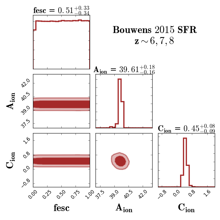
Figure 7: Bouwens et al. (2015) SFR observations, at z=6,7,8 combined together, constraints on our model parameters. Values on top of the 1-D PDFs diagonal represent the best fit parameters with 1-$\sigma$ (14th and 84th percentiles). Dark and light shaded regions correspond to 1-$\sigma$ and 2-$\sigma$ levels respectively. The Bouwens et al. (2015) SFR observations provide tight constraints on the ${A_{\rm ion}}$ and ${C_{\rm ion}}$ in the selected prior range. As expected, the SFR measurements don’t constrain the $f_{\mathrm{esc}}$.

Unlike other semi-numerical models that rely on the efficiency parameter $\zeta$, our model allows a direct comparison to the SFR measurements by using a parameterisation for ${R_{\rm ion}}$ that is directly relatable to SFR. For a consistent comparison with Bouwens et al. (2015) measurements, we convert the ${R_{\rm ion}}$ back to SFR using Equation (2) in Finlator et al. (2011) that is based on  Schaerer (2003) models, and add up all SFR from halos brighter than $\rm M_{AB}=-17$ at $z=6,7,8$. To compute the corresponding $\rm M_{AB}$, we use the linear relation provided in Kennicutt (1998) which converts the SFR to luminosity L_ν over the wavelength range 1500-2800 $\rm\AA$.

Figure 7 shows the posterior distribution of our parameters as constrained solely by Bouwens et al. (2015) integrated SFR observations at z=6,7,8 (taken together). This provides somewhat tigher constraints than fitting to a single redshift of SFR measurement, although constraining to a single redshift yields similar results, which indicates that the weak redshift evolution in the SFR measurements is adequately reproduced by our model for ${R_{\rm ion}}$.

The Bouwens et al. (2015) SFR observations provides tight constraints on the ${A_{\rm ion}}$ and ${C_{\rm ion}}$ as seen in figure 7. while poorly constraining $f_{\mathrm{esc}}$. The latter is expected because the $f_{\mathrm{esc}}$ is set by the recombinations in the ISM while the SFR depends on the halo mass and redshift.

The value of ${C_{\rm ion}}=0.45$ agrees within the 1-$\sigma$ level with what was previously found from fitting our hydrodynamical simulations, which yielded ${C_{\rm ion}}=0.41$ (Hassan et al., 2016). This means that our large volume semi-numerical model is compatible with the same slope of the ${R_{\rm ion}}$-$M_{h}$ relation predicted by the small volume 6/256-RT simulation to match the Bouwens et al. (2015) SFR observation, thereby nicely corroborating the direct simulation results.

However, the differences are more significant in the ${A_{\rm ion}}$ posterior distribution. We see that the ${A_{\rm ion}}$ best-fit value of 10^40.03 predicted by 6/256-RT simulation over-estimates by $\sim$ 50% the value of ${A_{\rm ion}}=10^{39.61}$ favoured by our SimFast21 MCMC fit using only the Bouwens et al. (2015) SFR constraints. This represents somewhat poor concordance at only a 3-$\sigma$ level. This discrepancy arises due to the small box size (=6h^-1Mpc) of 6/256-RT simulation that does not capture the large scale fluctuations and massive dark matter halos that contribute significantly to the reionisation photon budget. Hence, the 6/256-RT simulation requires larger ${A_{\rm ion}}$ to compensate for these limitations. This effect is also seen in figure 1 when comparing the reionisation histories of the 6/256-RT simulation with our large volume semi-numerical simulations which tend to reionise the universe much earlier at a fixed optical depth due to the presence of those massive halos and large scale-fluctuations.

Overall, utilising only the integrated SFR observations already gives interesting constraints on the slope and amplitude of the ionising photon output as a function of halo mass. However, there are no useful constraints on the escape fraction.

5.2.2 The Planck (2016) optical depth constraints

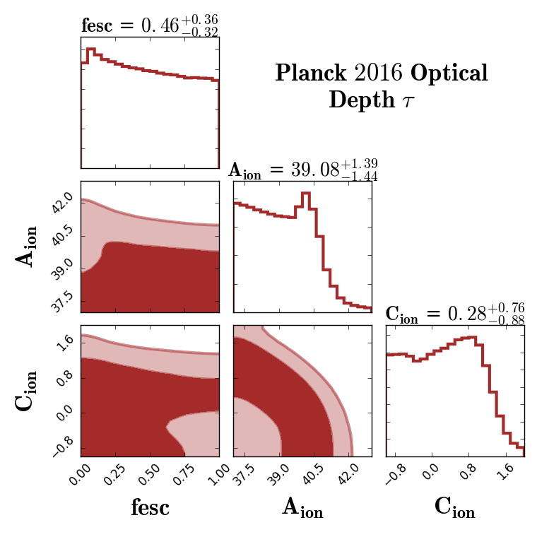
Figure 8: Planck (2016) optical depth constraints on our model parameters. Values on top of the 1-D PDFs diagonal represent the best fit parameters with 1-$\sigma$ (14th and 84th percentiles). Dark and light shaded regions correspond to 1-$\sigma$ and 2-$\sigma$ levels respectively. The Planck (2016) $\tau$ provides poor constraints on all parameters while there is slight tendency towards lower $f_{\mathrm{esc}}$ values. The Planck (2016) $\tau$ prefers models with low ${A_{\rm ion}}$ and ${C_{\rm ion}}$ values for the chosen prior range as compared to values implied by the Bouwens et al. (2015) SFR observations.

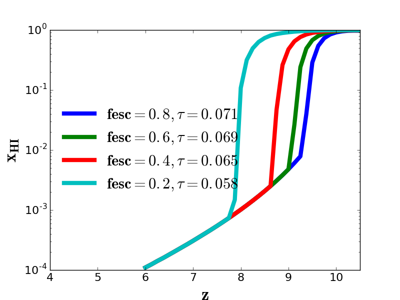
Figure 9: The reionisation history for our Time-integrated model with different $f_{\mathrm{esc}}$ values while fixing the ${A_{\rm ion}}$ and ${C_{\rm ion}}$ to values implied by the recent Planck (2016) $\tau$ measurements. This clearly shows that the current Planck (2016) optical depth $\tau=0.058\pm 0.012$ does not provide tight $f_{\mathrm{esc}}$ constraints for models with rapid reionisation scenarios as the case with our Time-integrated EoR model.

Figure 8 shows the parameters constrained to match solely the Planck (2016) data. This shows that the Thomson optical depth data alone provides fairly poor constraints on any of the parameters. There is a slight tendency to favour lower $f_{\mathrm{esc}}$ values, as also found by Greig & Mesinger (2016, see their Figure 4), but in general all values from zero to one are still allowed.

The main reason for the lack of sensitivity to $f_{\mathrm{esc}}$ is shown in Figure 9, and essentially arises from the still-large errors on $\tau$. Figure 9 shows the volume-weighted global neutral fraction evolution for fixed values of ${A_{\rm ion}}$ and ${C_{\rm ion}}$, and shows that $f_{\mathrm{esc}}=20\rightarrow 80$% gives rise to $\tau=0.058\rightarrow 0.071$, which is still essentially within the $1\sigma$ uncertainty on the measurement of $\tau=0.058\pm 0.012$. Hence much smaller error bars on $\tau$ are required to provide better constraints on $f_{\mathrm{esc}}$.

${A_{\rm ion}}$ and ${C_{\rm ion}}$ are also not well constrained by the Thomson optical depth data alone, though there is some tendency to favour small values of ${A_{\rm ion}}$ and ${C_{\rm ion}}$. Nonetheless, the uncertainties are large, and the values favoured from the SFR constraints alone are within the $1\sigma$ uncertainties of these predictions, as are the values found directly from the hydrodynamic simulations.

In summary, the Thomson optical depth as measured by Planck alone does not provide strong constraints on any of our parameters. It is clear that reducing uncertainties and/or including other data will be required in order to meaningfully constrain the sources driving reionisation.

5.2.3 The Becker & Bolton (2013) ionising emissivity constraints

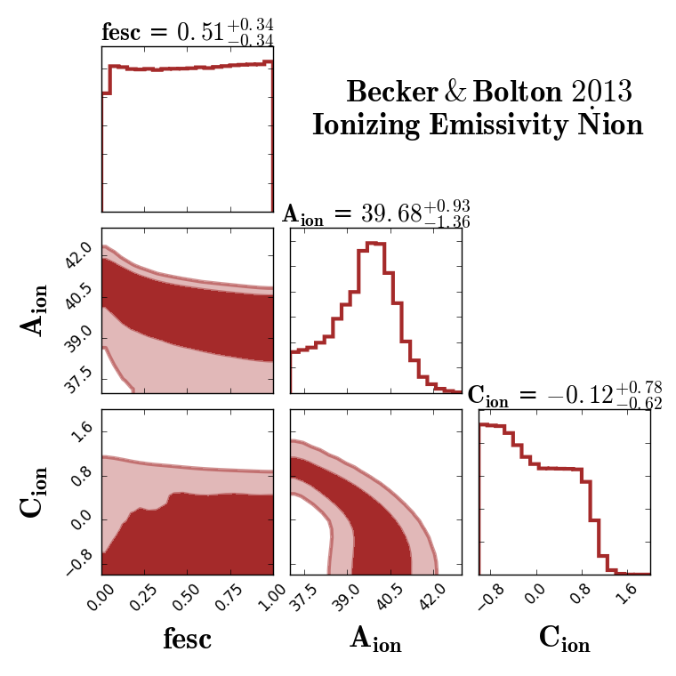
Figure 10: The Becker & Bolton (2013) ionising emissivity (z=4.75) constraints on our model parameters. Values on top of the 1-D PDFs diagonal represent the best fit parameters with 1-$\sigma$ (14th and 84th percentiles). Dark and light shaded regions correspond to 1-$\sigma$ and 2-$\sigma$ levels respectively. Similar to previous constraints, the $f_{\mathrm{esc}}$ is poorly constrained and similar to $\tau$ constraints, the data prefers lower $f_{\mathrm{esc}}$ values. The $\rm\dot{N}ion$ data also prefers models with negative ${C_{\rm ion}}$ in our selected prior range. This shows that matching to post-reionisation data requires fewer ionising photons and prefers models with dominant contributions from small dark matter halos.

The integrated emissivity of ionising photons $\rm\dot{N}_{ion}$ quantifies the total ionisation rate density from all ionising sources that escape galaxies to fill the intergalactic medium. Mathematically, $\rm\dot{N}_{ion}=\sum f_{\mathrm{esc}}{R_{\rm ion}}$ divided by the simulation’s comoving volume. To compare with Becker & Bolton (2013) $\rm\dot{N}ion$ measurements, we add up $f_{\mathrm{esc}}{R_{\rm ion}}$ from all halos and divide by the simulation comoving volume at z=4.75. As with the SFR data, our model permits a direct comparison with the $\rm\dot{N}ion$ data since we use a parameterisation for ${R_{\rm ion}}$ rather than a single efficiency parameter.

Figure 10 shows the posteriors for our three free parameters constrained only to match the Becker & Bolton (2013) $\rm\dot{N}ion$ data. As with the SFR and $\tau$ constraints, the $f_{\mathrm{esc}}$ is unconstrained by this data. Similar to Planck (2016) $\tau$ constraints, we find that models with high ${A_{\rm ion}}$ and ${C_{\rm ion}}$ values are disfavored by Becker & Bolton (2013) $\rm\dot{N}ion$ measurements, but again this is within $1\sigma$ of the SFR-only constraints.

The slight tendency of $\rm\dot{N}ion$ data towards negative values of ${C_{\rm ion}}$ (negative slope of ${R_{\rm ion}}$-$M_{h}$ relation) favours small halos being the dominant ionising photon sources contributor to match the post-reionisation measurements. In contrast, SFR and $\tau$ data prefers the positive side of ${C_{\rm ion}}$ values, implying that massive halos are more important during the reionisation. This shows that reionisation requires more ionising photons while matching post-reionisation data requires fewer ionising photons. This stands as one of the theoretical challenges for the EoR models as it is not easy to match simultaneously observational constraints during and after reionisations. $\rm\dot{N}ion$ measurements at higher redshifts ($z\sim\,6,7$) would be very useful to see if this tension extends into the overlapping redshift regime (Keating et al., 2014).

5.2.4 Combined SFR + $\bf\bf\tau$ + $\bf\bf\rm\dot{N}ion$ constraints

Figure 11: Combined constraints from SFR, $\bf\bf\tau$ and $\bf\bf\rm\dot{N}ion$. Values on top of the 1-D PDFs diagonal represent the best fit parameters with 1-$\sigma$ (14th and 84th percentiles). Dark and light shaded regions correspond to 1-$\sigma$ and 2-$\sigma$ levels respectively. Combining all these observations results in a tighter $f_{\mathrm{esc}}$ constraints while ${A_{\rm ion}}$ and ${C_{\rm ion}}$ still follow Bouwens et al. (2015) SFR constraints.

To obtain the strongest constraints given the observations we consider, we now combine our three key EoR constraints: the Bouwens et al. (2015) SFR observations, Planck (2016) optical depth measurements and the Becker & Bolton (2013) $\rm\dot{N}ion$ data. This represents the best available constraints we can make given current data, and serves to provide our base model from which we will do forecasting for 21cm experiments.

Figure 11 shows the parameter estimates as fit to the combined sample of these EoR observations. We see that the ${A_{\rm ion}}$ and ${C_{\rm ion}}$ are tightly constrained, which as Figure 7 showed is driven by the Bouwens et al. (2015) SFR constraints, as the other observations did not provide very tight constraints on these parameters.

The more interesting difference is in $f_{\mathrm{esc}}$, where the combined constraints now definitely prefers lower $f_{\mathrm{esc}}$ values, with best fit-value of $0.25^{+0.26}_{-0.13}$. This is still a rather wide range, and the posterior ellipses show that even very low escape fractions are not ruled out at more than a $\sim 1\sigma$ level, and very high $f_{\mathrm{esc}}$ values are only disfavoured at $\la 2\sigma$. This tendency was hinted at from matching to Becker & Bolton (2013) $\rm\dot{N}ion$ and Planck (2016) optical depth individually. This result indicates that our previous findings of $f_{\mathrm{esc}}=0.04-0.06$ in Hassan et al. (2016) is clearly possible for models with higher ${A_{\rm ion}}$ and ${C_{\rm ion}}$ values within their derived 1-$\sigma$ level. A summary of the individual and combined constraints is provided in Table 2.

This shows that current observations can already constrain the basic power law parameters of the ionising photon output versus halo mass, but constraints on $f_{\mathrm{esc}}$ are still somewhat elusive. Note that we are also assuming a constant $f_{\mathrm{esc}}$ for all galaxies, while there may be some mass and/or redshift dependence; however, with even a single parameter already being poorly constrained, it is unlikely that adding more parameters will allow tighter constraints.

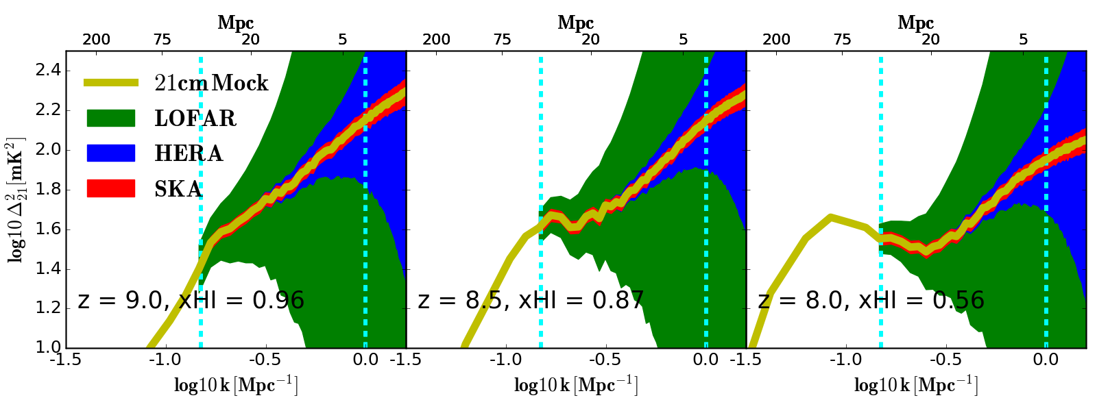
Figure 12: Three redshifts mock 21cm EoR observations using the well-calibrated Time-integrated EoR model with parameters ($f_{\mathrm{esc}},\,\rm log10(A_{ion}),\,C_{ion}$) = (0.24, 39.63, 0.43). Yellow solid line represents the 21cm power spectrum from the Large box mock observation (L=300/N=560). Shaded area shows the erorrbars obtained using 21cmSense package for our constructed EoR arrays: SKA (red), HERA (blue), LOFAR (green). Redshifts and neutral fractions for 21cm mock observations are quoted in each panel. Vertical cyan dashed lines show our chosen k-range to preform the 21cm MCMC.

6 21cm forecasting and experiments sensitivities

The ultimate goal is to add the 21cm observations to these existing data (or future improved versions thereof), in order to ascertain how well we can understand the sources of reionisation. To do so, we adopt a forecasting approach by which we use expected uncertainties from future 21cm power spectrum measurements in concert with these existing data and ascertain how much improvement the 21cm data will provide in the precision with which our parameters are constrained. We will assume a base model that is the best-fit to our current constraints as listed in Table 2.

We focus our analysis on LOFAR, HERA, and SKA1-Low. For each experiment, we first compute the thermal noise power spectrum which dominates the errors in measuring the 21cm signal. We then add more uncertainties from the sample variance, while neglecting the shot noise since it has been shown to have a minimal effect at the relevant scales ($k<2h$Mpc^-1) for these telescopes sensitivities (Pober et al., 2013). We obtain these uncertainties using the 21cmSense package, and refer to Parsons et al. (2012) for the full mathematical derivation of the radio interferometer sensitivities, and to  Pober et al. (2013, 2014) for more details on observation strategies and foreground removal models. We briefly highlight the basic equations and concepts used in 21cmSense to obtain the 21cm power spectrum error from a specific array configuration.

The dimensionless power spectrum of the thermal noise (Parsons et al., 2012; Pober et al., 2013, 2014) can be obtained using:

$$\Delta^{2}_{N}(k)\approx X^{2}Y\frac{k^{3}}{2\pi^{2}}\frac{\Omega}{2t}T^{2}_{sys}\,,$$ (7)

where $X^{2}Y$ is a conversion factor from angle and frequency units to comoving cosmological distances, $\Omega$ is the primary beam field-of-view, $t$ is the integration time and $T_{sys}$ is the system temperature (sky+receiver). It is then straightforward to add the sample variance to the thermal noise to obtain the total error (Pober et al., 2013) as follows:

$$\delta\Delta^{2}(k)=\left(\sum\frac{1}{\left(\Delta^{2}_{N}(k)+\Delta^{2}_{21}(k)\right)^{2}}\right)^{-\frac{1}{2}}\,,$$ (8)

where $\Delta^{2}_{21}$ is the 21cm power spectrum and the summation runs over all measured independent k-modes.

We construct these experiments as follows:

• LOFAR: We use the Netherlands 48 High-Band Antennas (HBA) with positions listed in van Haarlem et al. (2013) following Pober et al. (2014). Each antenna has a diameter of 30.75 m which results in a total collecting area of 35,762 m² for the 48 HBA station. The receiver temperature T_rcvr is set to 140,000 mK as suggested by Jensen et al. (2013); Greig & Mesinger (2015).

• HERA: We consider the final design of 331 hexagonally packed 14 m antennas (Ewall-Wice et al., 2016; Beardsley et al., 2015). With this configuration, the total collecting area becomes 50,953 m². We assume an 100,000 mK receiver temperature T_rcvr , similar to previous works by  Pober et al. (2014); Greig & Mesinger (2015).

• SKA-LOW1: We model SKA1-Low following the SKA1 System Baseline Design document by Dewdney (2013) in which the proposed array consists of 911 antennae in total. These antennae are distributed randomly to form a compact core using 866 dishes surrounded by the remaining 45 dishes along spiral arms. The 866 core antennae provide the vast majority of the sensitivity, and hence our SKA model ignores those 45 spiral arms stations (Pober et al., 2014; Greig & Mesinger, 2015). Each station of 866 antennae has a diameter of 35 m which makes a total collecting area of 833,189 m². The receiver noise here is determined by: T_rcvr = 0.1 T_sky + 40 K, where the sky temperature is modelled using: T_sky = 60$\lambda^{2.55}$.

For a consistent comparison, we choose to operate these three array designs in a drift-scanning mode for 6 observing hours per day for 180 days at 8 MHz bandwidth. We consider Pober et al. (2014) moderate foreground removal model where the foreground wedge extends 0.1 h Mpc^-1 beyond horizon limit.

	${\rm\bf f_{\mathrm{esc}}}$	${\rm\bf log10(A_{ion})}$	${\rm\bf C_{ion}}$
21cm Mock Observations
SKA	0.240${}^{+0.056}_{-0.054}$	39.628${}^{+0.030}_{-0.032}$	0.431${}^{+0.052}_{-0.056}$
HERA	0.237${}^{+0.061}_{-0.054}$	39.626${}^{+0.031}_{-0.025}$	0.425${}^{+0.055}_{-\textsection 0.058}$
LOFAR	0.415${}^{+0.384}_{-0.239}$	39.229${}^{+0.606}_{-1.117}$	0.445${}^{+0.341}_{-0.274}$
21cm Mock Observations + ALL (SFR, $\rm\bf\dot{N}_{ion}$, $\bf\rm\tau$)
SKA+ALL	0.217${}^{+0.052}_{-0.048}$	39.631${}^{+0.024}_{-0.029}$	0.423${}^{+0.053}_{-0.057}$
HERA+ALL	0.221${}^{+0.058}_{-0.051}$	39.630${}^{+0.029}_{-0.029}$	0.427${}^{+0.053}_{-0.059}$
LOFAr+ALL	0.206${}^{+0.069}_{-0.045}$	39.634${}^{+0.042}_{-0.033}$	0.421${}^{+0.065}_{-0.060}$

Table 3: Summary of our parameter estimations from the 21cm mock observations and from combining the 21cm mock observations with the current EoR observations (SFR, $\rm\bf\dot{N}_{ion}$, $\bf\rm\tau$).

6.1 Including the 21cm data

We combine three different redshifts of 21cm power spectrum observations, namely $z=9.0,8.5,8.0$, which provides tighter constraints than considering any single epoch observations. With multiple redshifts 21cm observations, one accounts simultaneously for the variation in redshift (density field) and neutral fraction (ionisation field) evolution, which are the main components in determining the 21cm fluctuations. Given the rapid reionisation behaviour of the Time-integrated model as shown in figure 1, our selected redshifts ($z=9,8.5,8$) correspond to a wide range of neutral fractions that account for different reionisation epochs such as the initial bubble growth and the bubble overlap phase. We next construct the likelihood from these observations by simply adding up their individual $\chi^{2}$. We limit our analysis to a wide $k$-range of 0.15-1.0 Mpc^-1, consistent with Greig & Mesinger (2015). From this $k$-range, we select 10 bins of the power spectrum which is sufficient to capture the fluctuations for a given 21cm power spectrum.

We use the well-calibrated Time-integrated model with parameters derived from fitting to our combined set of EoR observations as discussed in § 5.2.4 and shown in figure 11. Specifically, we use the following parameters: ($f_{\mathrm{esc}},\,\rm log10(A_{ion}),\,C_{ion}$) = (0.24, 39.63, 0.43), consistent with the 1-$\sigma$ level of constraints by our combined set of EoR observations. We then use these parameters to create our mock observations with a large box size of $L=300$ Mpc and $N=560$ per side which results in a resolution of 0.375 $h^{-1}$ Mpc. We determine the error in measuring the 21cm power spectra for our mock observation by using the telescope sensitivity code 21cmSense for each specific array experiments at our chosen redshifts as described above. We use the same pipeline discussed in § 5.1 to sample the 21cm power spectrum space, except now we include the 21cm mock observation power spectra among the pre-computed runs to study how well the MCMC technique may recover the input model parameters.

Figure 12 shows our 21cm mock observations at several redshifts. The shaded area corresponds to the error in measuring the 21cm power spectrum for our large mock observations using the 21cmSense package. LOFAR (green shading), operating currently, will be able to constrain only the largest scales considered here, while HERA (blue), under construction now, will be further sensitive to intermediate scales, while the future SKA1-Low (red) will provide tight constraints into the sub-Mpc scale regime owing to its wider baselines and hence better resolution. These uncertainties depend mainly on our telescope configurations as described above. Hence the main improvement as these facilities develop will be to better constrain the 21cm power spectrum towards smaller scales, and each generation will provide significant gains in this.

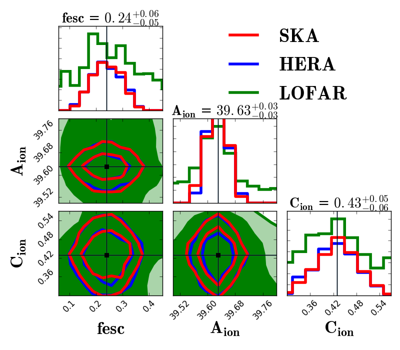
Figure 13: 21cm power spectrum constraints on our three EoR parameters from several redshifts (z=9.0,8.5,8.0) mock observations. SKA, HERA, and LOFAR constraints are shown by red, blue, and green contours respectively. Values on top of the 1D PDFs represent the best fit parameters as implied by the SKA mock observations while black square points correspond to the input mock observation parameters: ($f_{\mathrm{esc}},\,\rm log10(A_{ion}),\,C_{ion}$) = (0.24, 39.63, 0.43). The MCMC technique is able to recover the input model parameters. It is evident that the future 21cm observations can tightly constrain our model parameters for experiments with small and intermediate levels of uncertainty in detecting the expected signal such as SKA and HERA respectively.

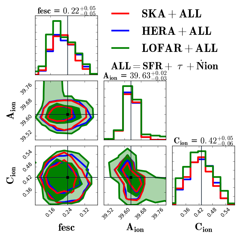
Figure 14: Parameter estimates from combining the current EoR observations with the 21cm mock observations. The current EoR observations here are our previous combined sample: SFR, $\bf\bf\tau$ and $\bf\bf\rm\dot{N}ion$ while the 21cm mock observations are combinations of several 21cm redshifts at z=9.0,8.5,8.0. SKA, HERA, and LOFAR constraints are shown by red, blue, and green contours respectively. Values on top of the 1D PDFs represent the best fit parameters as implied by the SKA mock observations while black square points correspond to the input mock observation parameters: ($f_{\mathrm{esc}},\,\rm log10(A_{ion}),\,C_{ion}$) = (0.24, 39.63, 0.43). It is evident that adding the current EoR observations on top of the 21cm mock observations provide more tighter constraints even for experiments with large 21cm power uncertainties such as the case with LOFAR.

6.2 21cm MCMC

We now ask how well the 21cm data can constrain our free parameters. First, we consider the 21cm power spectrum data as shown in Figure 13 by itself, to see how tightly our parameters can be constrained by such observations alone. Then we add the 21cm data to our other existing observational constraints. In each case we use our MCMC framework to determine our best-fit values of our free parameters and their uncertainties using the entire data set, for the case of each telescope facility. This provides forecasting for how much improvement can be expected from future 21cm observations.

Figure 13 shows the 1D PDFs and 2D contours of our three parameters from the combined redshifts ($z=9.0,8.5,8.0$) of 21cm mock observations by our three selected EoR experiments. To begin, we see that our MCMC search well recovers the best-fit input model (mock observation) parameters (black square points). This is to be expected, since this same input model was used to generate the 21cm data. The improvement to be noted here is the reduction of the uncertainties on these parameters relative to the previous case without 21cm data.

For LOFAR (green shaded area), we see that the 21cm observations don’t provide tight constraints due to large uncertainties as seen in figure 12. Essentially, mildly constraining the large-scale power provides little information on the ionisation sources that drive reionisation.

In contrast, HERA (blue) and SKA (red) provide quite tight constraints on the free parameters. Note that the scale of the posteriors is substantially reduced relative to our previous plots in order to enhance visibility. Hence future 21cm data alone can already independently constrain reionising sources, without adding in any other observations. Interestingly, there is almost no difference between the SKA and HERA constraints. This arises because the parameter constraints are predominantly driven by the larger scales, and HERA and SKA provide similar constraints on the power spectrum for scales $\ga 2$ Mpc.

Comparing the 21cm constraints with constraints obtained from combining several EoR key observables, we find that constraining to 21cm observations yield smaller parameter errors. This can be clearly seen when comparing the 1-$\sigma$ level of $f_{\mathrm{esc}}$ and ${A_{\rm ion}}$ found by constraining to the 21cm observations (fig 13) versus to the combined EoR sample (SFR, $\rm\dot{N}_{ion}$, $\tau$) (fig 11). However, it is evident that the 21cm future observation can constrain the $f_{\mathrm{esc}}$ tighter than the current EoR key observables.

In previous work by  Greig & Mesinger (2015), the authors used a similar semi-numerical framework and performed similar analysis to constrain their free parameters to future 21cm mock observations. However, they did not have the photon escape fraction as a free parameter and rather constrained their efficiency parameter $\zeta$, from which the $f_{\mathrm{esc}}$ can be computed for various assumptions about gas fraction in stars and ionising photons number per baryons (see their eq. (2)). However, we here constrain the $f_{\mathrm{esc}}$ directly without making further assumptions about the gas and baryons fractions, hence our presented $f_{\mathrm{esc}}$ results are direct, albeit the inherent photon conservation issues in these semi-numerical models, which we will discuss later.

We finally constrain our free parameters by combining the 21cm mock observations with the current EoR key observables (SFR, $\rm\dot{N}_{ion}$, $\tau$) as shown in figure 14. From this figure, we see that our three parameters are well-constrained by the combined set of current EoR and 21cm mock observations. Adding our combined EoR sample (SFR, $\rm\dot{N}_{ion}$, $\tau$) on top of the 21cm mock observations improves the error in estimating our free parameters, particularly for arrays with large 21cm errorbars such as LOFAR. This shows that the future 21cm observations are important in constraining the model astrophysical parameters and complement the other existing EoR various observations. A summary of our 21cm mock observations constraints combined with the other EoR observations is given in table 3.

Our 21cm forecasting shows that the future 21cm power spectrum observations will be crucial for providing tight constraints on various parameters related to the sources of reionisation. Even by themselves, such data will provide improve constraints over what can be obtained using current observations. When combined with other observations, the constraints get quite tight, even for the difficult-to-constrain photon escape fractions $f_{\mathrm{esc}}$. The tightness of the constraints suggest that it may be possible to independently constrain variations in the escape fraction with mass or redshift; we will examine this in future work.

6.3 Photon conservation

To make use of our $f_{\mathrm{esc}}$ constraints, we here test the photon conservation problem in our semi-numerical model. Previous semi-numerical models, based on the excursion set formalism, have pointed out a violation in the photon number conservation. In Zahn et al (2007), the authors found that their semi-numerical model loses about 20% photons. They have argued that this photon loss arises from ionised bubbles overlapping, which they compensated by boosting the efficiency parameter $\zeta$. More recent work by Paranjape et al. (2016) have developed a Monte Carlo Model of bubble growth to resolve the photon conservation problem in their semi-numerical model. Although their bubble growth model didn’t resolve the problem completely, nevertheless improvements have been achieved and they have demonstrated that the problem comes from the fact that the excursion set-based models use the average mass of the bubbles rather than tracking the actual mass of sources and bubble local density fluctuations.

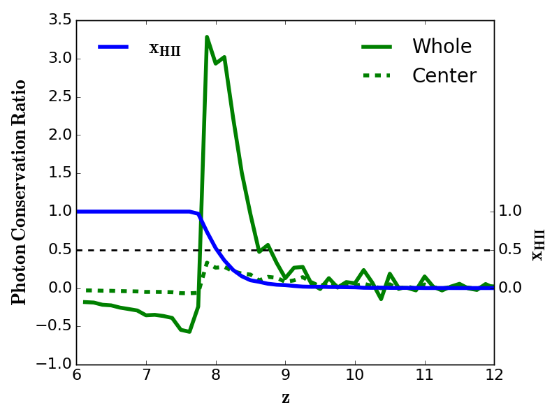
Figure 15: Photon conservation ratio from the Time-integrated EoR model using whole flagging (green solid) versus center flagging (greed dashed) scheme, with their reionisation history (blue solid). Horizontal black dashed line represents the 50% neutral/ionised fraction limit. Both methods violate the photons number conservations as seen by the under-ionisation at high redshifts and over-ionisation at end of reionisation.

However, there are two methods to flag the spherical regions as ionised in the excursion set-formalism. The first is to flag the whole cells in the bubble (whole flagging) whereas the second is to flag only the center cell of the bubble (center flagging). We next use these two methods to verify the photon conservation in our Time-integrated EoR model. We would expect that, during time interval $\rm dt$, the total number of escaped ionising photons ($\rm f_{\mathrm{esc}}{R_{\rm ion}}\,dt$) minus the total number of recombinations ($\rm{R_{\rm rec}}\,dt$) should be equal to the number of ionisations in the neutral hydrogen atoms ($\rm(x_{HII}(t_{i+1})-x_{HII}(t_{i}))N_{H}$). In other words, the successful photons that manage to escape from the interstellar medium (corrected by $f_{\mathrm{esc}}$) and from high density regions along the way (subtracted by $\rm{R_{\rm rec}}\,dt$) should be equal to the total number of neutral atoms that have been ionised during time $\rm dt$. We can write the photon conservation ratio as follows:

$$\rm Photon\,Conservation\,Ratio\,=\frac{(x_{HII}(t_{i+1})-x_{HII}(t_{i}))N_{H}}{(f_{\mathrm{esc}}{R_{\rm ion}}-{R_{\rm rec}})\,dt},$$ (9)

where $\rm dt=t_{i+1}-t_{i}$. This ratio should be equal to unity for an ideal photon conserving model. However, the ratio can be less than unity when the universe is highly ionised. We then apply this ratio to the two methods, whole flagging versus center flagging, to check the photon conservation problem in both. We note that center flagging scheme requires about 20% more ionising photons to match the reionisation history obtained by whole flagging method. We then adjust the $f_{\mathrm{esc}}$ in two methods to reproduce identical reionisation history (identical $\tau$) while keeping other parameters fixed.

In figure 15. we plot the photon conservation ratio for the two methods, whole flagging (green solid line) and center flagging (green dashed line) with the reionisation history (blue solid line). We find that the center flagging scheme under-uses photons during all reionisation redshifts, even after reionisation (z $<$ 8), which might partly explain the need for higher $f_{\mathrm{esc}}$ with this method. The photon loss in the whole flagging scheme agrees qualitatively with center flagging at higher redshifts when the universe is almost neutral.

As reionisation proceeds, the whole flagging starts to over-use photons and ionises more neutral atoms than expected. The photon excess/loss in the two methods are clearly redshift dependent. In the center flagging method, the photon loss is by a factor of $\sim$ 3,7,20 at z= 7.75, 9.25, 11 respectively. The whole flagging scheme shows photon loss (under-using photons) at high redshifts and photon excess (over-using photons) at the end of reionisation. At high redshifts, the photon loss, in the whole flagging, is by a factor of $\sim$ 2,4,7 at z= 8.75,9,11 respectively. This shows that, at high redshifts, the photon loss, in the whole flagging method, is less by a factor of $\sim$ 2,3 as compared with center flagging method. At z=8.5 ($\rm x_{HI}\sim$ 0.9), the whole flagging method satisfies the photon conservation condition as the ratio becomes unity, but the ratio does not converge at unity afterwards. After this point, the whole flagging scheme starts to overuse photons increasingly by a large amount till the end of reionisation. We find the photon excess is about 10% at z=8.4 and 70% at z=7.75 (end of reionisation).

We note that all our EoR models adopts the whole flagging method. This shows that our constrained photon escape fractions $f_{\mathrm{esc}}$ are, in fact, over-estimated by the photon excess associated with the whole flagging method. All our previous $f_{\mathrm{esc}}$ estimations can be corrected and lowered by 10% up to 70% depending on redshifts. The photon loss/excess evolution in redshift suggests that the $f_{\mathrm{esc}}$ might be required to change with redshift in order to preserve photon number conservation as a temporary solution.

7 conclusion

We have improved our SimFast21 semi-numerical code for computing the EoR on large scales by incorporating a more physically-motivated criterion for determining whether a region of space is ionised, as well as integrating our framework into a full MCMC parameter search framework so we can forecast how well current and future observations can constrain the physical properties of the sources driving reionisation.

We have calibrated our new model to various current observations of the EoR, namely the Bouwens et al. (2015) SFR observations, the Planck (2016) optical depth measurements, and the Becker & Bolton (2013) $\rm\dot{N}ion$ data. We also compared our new EoR model to our previous EoR model in Hassan et al. (2016) in terms of their EoR history, H ii bubble sizes, and 21cm power spectra. We further studied variations in the 21cm fluctuations produced by all possible variants of our ionisation conditions.

We then presented a robust MCMC analysis to constrain our generalized source model’s free parameters against current EoR observations. We used the well-calibrated EoR model to predict the 21cm power spectrum for the future EoR array experiments SKA, HERA, and LOFAR. We show how the future 21cm observations are important for complementing the existing EoR current observations in order to tightly estimate the astrophysical parameters of EoR sources.

Our key findings are as follows:

• The Time-integrated EoR model produces very large H ii bubbles as compared with the Instantaneous EoR model, and fewer small bubbles. This difference is clearly shown in their evolving HI maps (figure 2) and the ionisation field (figure 3). This results in a larger ionisation and 21cm power spectrum on large scales by 1-1.2 orders of magnitude as seen in (Figure 4 and  5).

• By considering all possible combinations between the hydrogen atoms and recombination terms in the ionisation condition, we showed that recombinations are subdominant in determining the 21cm power spectrum particularly on large scales (Figure 6). The 21cm power spectrum amplitude and shape are highly sensitive to accounting for the amount of and fluctuations in the neutral hydrogen density. This means semi-numerical models must carefully account for the neutral hydrogen to robustly predict the expected 21cm signal.

• The Bouwens et al. (2015) SFR observations provide tight constraints on the ionising emissivity amplitude ${A_{\rm ion}}$ and the slope of the ${R_{\rm ion}}$-M_h relation ${C_{\rm ion}}$, but provide no constraint on the photon escape fraction $f_{\mathrm{esc}}$ (Figure 7). The recent Planck (2016) optical depth (Figure 8) and the Becker & Bolton (2013) $\rm\dot{N}ion$ measurements (Figure 10) poorly constrain our model parameters, while they slightly prefers models with lower values of $f_{\mathrm{esc}}$, ${A_{\rm ion}}$ and ${C_{\rm ion}}$.

• Combining all of SFR, $\tau$ and $\rm\dot{N}ion$ together results in tighter parameter constraints, as seen in Figure 11. The ${A_{\rm ion}}$ and ${C_{\rm ion}}$ here follow the previous constraints by the SFR observations, but combining these measurements yields better escape fraction constraints of $f_{\mathrm{esc}}=0.25^{+0.26}_{-0.13}$, though still not very tight. The parameters determined directly from the full hydrodynamic simulations analysed in Hassan et al. (2016) are consistent with these constraints.

• Using the well-calibrated Time-integrated EoR model, we predict the 21cm power spectrum at different redshifts ($z=9,8.5,8$) for several constructed radio array designs, namely SKA, HERA, and LOFAR (Figure 12). While LOFAR does not provide strong constraints except at the largest scales, future experiments will tightly constrain the 21cm power spectrum to smaller scales that can better constrain the reionising source population.

• By adding current EoR observations (SFR, $\tau$, $\rm\dot{N}ion$) to the 21cm mock observations, we find that all experiments recovers the input model parameter accurately and the parameters error are futher improved. This illustrates how future 21cm observations can complement and substantially improve upon existing EoR observations in order to more tightly constrain the emissivity of EoR sources and their relationship to the underlying halo population.

• We find that photon conservation is sub-optimal owing to the way the excursion set formalism is generically implemented in current semi-numerical codes, including SimFast21. The root difficulty is that cells are treated as fully neutral or fully ionised, with no possibility of intermediate ionisation levels. While some tuning could be done to minimise the problem, a robust solution likely lies in replacing the excursion set-formalism with a proper photon-conserving radiative transfer approach. We leave this for future work.

We have discussed the uncertainty associated with ionization condition in the excursion set-based models and found that a slight change in the ionization condition could lead to a big difference in the 21cm power spectrum particularly on large scales as seen between the Time-integrated and Instantaneous model. A possible approach to break such degeneracy and resolve the ionization condition uncertainty is to compare these models’ 21cm power spectra to radiative transfer simulations. For this reason, we are currently developing our own radiative transfer routine (SimFast21-RT) and the result will be forthcoming.

The SimFast21-MCMC platform developed here will be applicable for a wide range of EoR forecasting science cases. By robustly incorporating all the current observables within an MCMC framework and being able to straightforwardly incorporate new data, we are building the tools necessary to optimally connect future redshifted 21cm power spectrum from the EoR to physical quantities associated with the population of reionising sources. Such a framework can be used to explore and constrain exotic source populations such as mini-quasars or Population III stars, as well as to potentially extend to multi-tracer cross-correlation approaches. The most immediate hurdle will be to develop a more robust yet still fast radiative transfer method that conserves photons, so we can more reliably assess the obtained source population parameters. There is much exciting work to be done as we continue to prepare for the 21cm EoR era.

Appendix A REIONIZATION HISTORY CONVERGENCE TEST

As mentioned earlier, our new Time-integrated EoR model is sensitive to the choice of simulation time step dz, due to implementing time-integrated ionisation condition (equation 5). The correct reionisation history is however achieved for very small values of dz (ideally when dz goes to zero), which is computationally impossible. We here present a convergence test to support our choice of dz=0.125. Figure 16 shows the well-calibrated Time-integrated model reionisation history for different time steps dz using a simulation box size of L=75 Mpc and N=140³. It is clear that the reionisation starts earlier (higher $\tau$) when adopting larger steps (dz = 1.0 in black or 0.5 in yellow) than using smaller step values (dz $\leqslant$ 0.25). This means using larger dz permits more ionising photons production, and hence lower neutral fractions as seen in the beginning of the reionisation.

Comparing the reionisation history obtained with dz = 0.125 (cyan) versus that with dz = 0.01 (blue, the most correct result), we find both models produce similar tau ($\rm\Delta\tau\sim 0.001$) and the reionisation history shape is identical. There is a very minor difference in the neutral fraction of $\rm\Delta x_{HI}\sim 0.01$ by end of reionisation. Hence we conclude that our Time-integrated model is numerically well converged for dz $\leqslant$ 0.125.

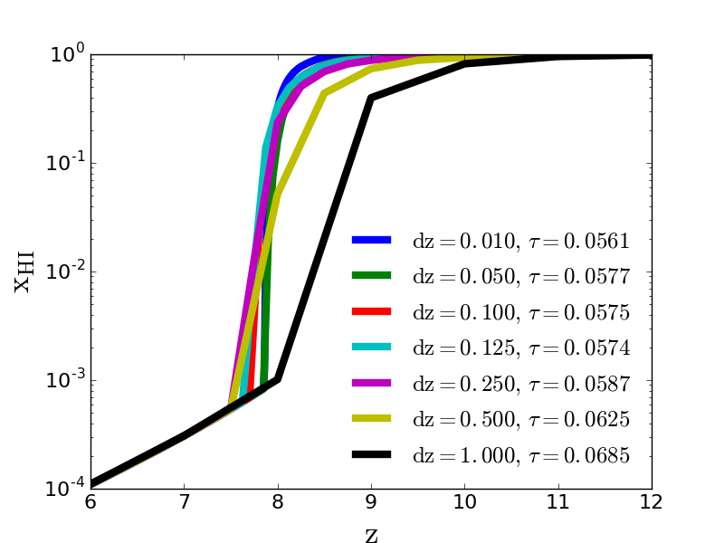
Figure 16: Reionisation history convergence test in our new Time-integrated EoR model using different time interval steps as quoted in the legend along with the corresponding optical depth. It is evident that our model is well converged for dz $\leqslant$ 0.125.

References

- Akeret et al. (2013) Akeret J., Seehars S., Amara A., Refregier A., Csillaghy A., 2013, Astronomy and Computing, 2, 27
- Barkana & Loeb (2001) Barkana, R. & Loeb, A. 2001, Phys. Rep., 349, 125
- Bauer et al. (2015) Bauer, A., Springel, V., Vogelsberger, M., Genel, S., Torrey, P., Sijacki, D., Nelson, D., Hernquist, L., 2015, MNRAS, 453, 3593.
- Beardsley et al. (2015) Beardsley, A. P., Morales, M. F., Lidz, A., Malloy, M., Sutter, P. M., 2015, ApJ, 800, 128.
- Becker & Bolton (2013) Becker, G. D., Bolton, J. S. 2013, MNRAS, 436, 1023
- Bouwens et al. (2015) Bouwens J. R., Illingworth D. G., Oesch A. P., Trenti M., Labé I., Bradley L., Carollo M., Van Dokkum G. P., Gonzalez V., Holwerda B., Franx M., Spitler L., Smit R., Magee D., 2015, ApJ, 803, 34.
- Bouwens et al. (2015) Bouwens, R. J., Illingworth, G. D., Oesch, P. A., et al., 2015, ApJ, 811, 140,
- Choudhury et al (2009) Choudhury T. R., Haehnelt M. G., Regan J., 2009, MNRAS, 394, 960
- Davé et al. (2013) Davé, R., Katz, N., Oppenheimer, B. D., Kollmeier, J. A., Weinberg, D. H. 2013, MNRAS, 434, 2645
- Dewdney (2013) Dewdney P. E., 2013, Technical report, SKA1 SYSTEM BASELINE DESIGN.
- Ewall-Wice et al. (2016) Ewall-Wice, A. et al, 2016, MNRAS, 460, 4320
- Fan et al (2006) Fan, X., Carilli, C.L., Keating B. 2006, Annual Review of Astronomy and Astrophysics, 44, 415
- Feroz et al. (2009) Feroz, F., Hobson, M. P., Bridges, M., 2009, MNRAS, 398, 1601.
- Finlator & Davé (2009) Finlator, K. Özel, F. & Davé, R. 2009, MNRAS, 393, 1090
- Finlator et al. (2011) Finlator, K., Davé, R., Özel, F. 2011, 743, 169
- Finlator et al. (2013) Finlator, Kristian; Muñoz, Joseph A.; Oppenheimer, B. D.; Oh, S. Peng; Özel, F. & Davé, 2013, MNRAS, 436, 1818
- Finlator et al. (2015) Finlator, K., Thompson, R., Huang, S., Davé, R., Zackrisson, E., Oppenheimer, B. D. 2015, MNRAS, 447, 2526
- Foreman-Mackey et al. (2013) Foreman-Mackey D., Hogg D. W., Lang D., Goodman J., 2013, PASP, 125, 306
- Foreman-Mackey (2016) Foreman-Mackey, D., 2016, JOSS, 24.
- Gnedin (2000) Gnedin, N. Y. 2000, ApJ, 542, 535
- Gnedin (2014) Gnedin, N. Y., 2014, ApJ, 793, 29.
- Greig & Mesinger (2015) Greig, B.; Mesinger, A., 2015, MNRAS, 449, 4246.
- Greig & Mesinger (2016) Greig, B.; Mesinger, A., 2016, arXiv:1605.05374
- Hassan et al. (2016) Hassan, S. and Davé, R. and Finlator, K. and Santos, M. G., 2016, MNRAS, 457, 1550
- Hinshaw et al. (2013) Hinshaw, G. et al. 2013, ApJS, 208, 19
- Iliev et al. (2014) Iliev, I. T., Mellema, G., Ahn, K., et al. 2014, MNRAS, 439, 725
- Iliev et al. (2015) Iliev, Ilian T.; Santos, Mario G.; Mesinger, Andrei; Majumdar, Suman; Mellema, Garrelt; 2015 Proc. Sci., Epoch of Reionisation modelling and simulations for SKA. SISSA, Trieste, PoS (AASKA14) 007.
- Jensen et al. (2013) Jensen, H. et al, 2013, MNRAS, 435, 460.
- Katz et al. (2016) Katz, H, Kimm, T., Sijacki, D., Haehnelt, M., 2016, arXiv:1612.01786.
- Keating et al. (2014) Keating, L. C., Haehnelt, M. G., Becker, G. D., Bolton, J. S., 2014, MNRAS, 438, 1820.
- Kennicutt (1998) Kennicutt, Jr., R. C. 1998, ARA&A, 36, 189
- Kulkarni et al. (2016) Kulkarni, G., Choudhury, T. R., Puchwein, E., Haehnelt, M. G., 2016, MNRAS, 463, 2583.
- Majumdar et al. (2014) Majumdar S., Mellema G., Datta K. K., Jensen H., Choudhury T. R., Bharadwaj S., Friedrich M. M., 2014, ArXiv e-prints, arXiv:1403.0941
- Mesinger & Furlanetto (2007) Mesinger A., Furlanetto S., 2007, ApJ, 669, 663
- Mesinger et al. (2011) Mesinger, A.; Furlanetto, S.; Cen, R. 2011, 411, 955.
- Mitra et al. (2011) Mitra, S., Choudhury T. R., Ferrara A., 2011, MNRAS, 413, 1569.
- Mitra et al. (2012) Mitra, S., Choudhury T. R., Ferrara A., 2012, MNRAS, 419, 1480.
- Mitra et al. (2013) Mitra, S., Ferrara, A., & Choudhury, T. R. 2013, MNRAS, 428, L1
- Mitra et al. (2015) Mitra S, Choudhury T. R., Ferrara A. 2015, arXiv:1505.05507
- Mellema et al (2006) Mellema, G., Iliev, I. T., Pen, U.-L., & Shapiro, P. R. 2006, MNRAS, 372, 679
- McQuinn et al (2007) McQuinn, M., Lidz, A., Zahn, O., et al. 2007, MNRAS, 377, 1043
- Paranjape et al. (2016) Paranjape, A., Choudhury, T. R, Padmanabhan, H., 2016, MNRAS, 460, 1801.
- Parsons et al. (2012) Parsons, A., Pober, J., McQuinn, M., Jacobs, D., Aguirre, J., 2012, ApJ, 753, 81.
- Pawlik & Schaye (2008) Pawlik, A. H.; Schaye, J., 2008, MNRAS, 389, 651
- Pentericci et al. (2014) Pentericci, L. et al. 2014, ApJ, 793, 113
- Pober et al. (2013) Pober, J. C., Parsons, A. R. et al, 2013, AJ, 145, 65.
- Pober et al. (2014) Pober, J. C., Liu, A. et al, 2014, ApJ, 782, 66.
- Razoumov et al (2002) Razoumov, A. O., Norman, M. L., Abel, T., & Scott, D. 2002, ApJ, 572, 695
- Planck (2015) Planck Collaboration XIII, Ade, P. A. R., Aghanim, N., et al. 2015, arXiv:1502.01589 [PC15]
- Planck (2016) Planck intermediate results. XLVII, Adam, R., Aghanim, N., et al 2016, arXiv:1605.03507
- Santos et al. (2010) Santos M. G., Ferramacho L., Silva M. B., Amblard A., Cooray A. 2010, MNRAS, 406, 2421
- Sobacchi & Mesinger (2014) Sobacchi E., Mesinger A., 2014, MNRAS, 440, 1662
- Schaerer (2003) Schaerer, D. 2003, A&A, 397, 527
- Thomas et al (2009) Thomas, R. M., Zaroubi, S., Ciardi, B., et al. 2009, MNRAS, 393, 32
- van Haarlem et al. (2013) van Haarlem, M. P. et al, 2013, A&A, 556, 2.
- Zel’Dovich (1970) Zel’Dovich Y. B., 1970, A&A, 5, 84
- Zahn et al (2007) Zahn O., Lidz A., McQuinn M., Dutta S., Hernquist L., Zaldarriaga M., Furlanetto S. R., 2007, ApJ, 654, 12
- Zahn et al (2011) Zahn O., Mesinger A., McQuinn M., Trac H., Cen R., Hernquist L. E., 2011, MNRAS, 414, 727