Abstract

We describe the new version (v2.73y) of the code hfodd which solves the nuclear Skyrme Hartree-Fock or Skyrme Hartree-Fock-Bogolyubov problem by using the Cartesian deformed harmonic-oscillator basis. In the new version, we have implemented the following new features: (i) full proton-neutron mixing in the particle-hole channel for Skyrme functionals, (ii) the Gogny force in both particle-hole and particle-particle channels, (iii) linear multi-constraint method at finite temperature, (iv) fission toolkit including the constraint on the number of particles in the neck between two fragments, calculation of the interaction energy between fragments, and calculation of the nuclear and Coulomb energy of each fragment, (v) the new version 200d of the code hfbtho, together with an enhanced interface between hfbtho and hfodd, (vi) parallel capabilities, significantly extended by adding several restart options for large-scale jobs, (vii) the Lipkin translational energy correction method with pairing, (viii) higher-order Lipkin particle-number corrections, (ix) interface to a program plotting single-particle energies or Routhians, (x) strong-force isospin-symmetry-breaking terms, and (xi) the Augmented Lagrangian Method for calculations with 3D constraints on angular momentum and isospin. Finally, an important bug related to the calculation of the entropy at finite temperature and several other little significant errors of the previous published version were corrected.  

PACS numbers: 07.05.T, 21.60.-n, 21.60.Jz

NEW VERSION PROGRAM SUMMARY

Title of the program: hfodd (v2.73y)

Catalogue number: ….

Program obtainable from: CPC Program Library,  Queen’s University of Belfast, N. Ireland (see application form in this issue)

Reference in CPC for earlier version of program: N. Schunck, J. Dobaczewski, J. McDonnell, W. Satuła, J. Sheikh, A. Staszczak, M. Stoitsov, and P. Toivanen, Comput. Phys. Commun. 183 (2012) 166-192.

Catalogue number of previous version: ADFL_v2_1

Licensing provisions: GPL v3

Does the new version supersede the previous one: yes

Computers on which the program has been tested: Intel Pentium-III, Intel Xeon, AMD-Athlon, AMD-Opteron, Cray XT4, Cray XT5

Operating systems: UNIX, LINUX, Windows${}^{\text{xp}}$

Programming language used: FORTRAN-90

Memory required to execute with typical data: 10 Mwords

No. of bits in a word: The code is written in single-precision for the use on a 64-bit processor. The compiler option -r8 or +autodblpad (or equivalent) must be used to promote all real and complex single-precision floating-point items to double precision when the code is used on a 32-bit machine.

Has the code been vectorised?: Yes

Has the code been parallelized?: Yes

No. of lines in distributed program: 159 633 (of which 62 714 are comments and separators)

Keywords: Hartree-Fock; Hartree-Fock-Bogolyubov; Skyrme interaction; Self-consistent mean field; Nuclear many-body problem; Superdeformation; Quadrupole deformation; Octupole deformation; Pairing; Nuclear radii; Single-particle spectra; Nuclear rotation; High-spin states; Moments of inertia; Level crossings; Harmonic oscillator; Coulomb field; Pairing; Point symmetries; Yukawa interaction; Angular-momentum projection; Generator Coordinate Method; Schiff moments; Isospin mixing; Isospin projection, Finite temperature; Shell correction; Lipkin method; Multi-threading; Hybrid programming model; High-performance computing.

Nature of physical problem

The nuclear mean field and an analysis of its symmetries in realistic cases are the main ingredients of a description of nuclear states. Within the Local Density Approximation, or for a zero-range velocity-dependent Skyrme interaction, the nuclear mean field is local and velocity dependent. The locality allows for an effective and fast solution of the self-consistent Hartree-Fock equations, even for heavy nuclei, and for various nucleonic ($n$-particle $n$-hole) configurations, deformations, excitation energies, or angular momenta. Similarly, Local Density Approximation in the particle-particle channel, which is equivalent to using a zero-range interaction, allows for a simple implementation of pairing effects within the Hartree-Fock-Bogolyubov method. For finite-range interactions, like Coulomb, Yukawa, or Gogny interaction, the nuclear mean field becomes nonlocal, but using the spatial separability of the deformed harmonic-oscillator basis in three Cartesian directions, the self-consistent calculations can be efficiently performed.

Method of solution

The program uses the Cartesian harmonic oscillator basis to expand single-particle or single-quasiparticle wave functions of neutrons and protons interacting by means of the Skyrme or Gogny effective interactions and zero-range or finite-range pairing interactions. The expansion coefficients are determined by the iterative diagonalization of the mean-field Hamiltonians or Routhians which depend non-linearly on the local or nonlocal neutron, proton, or mixed proton-neutron densities. Suitable constraints are used to obtain states corresponding to a given configuration, deformation or angular momentum. The method of solution has been presented in: J. Dobaczewski and J. Dudek, Comput. Phys. Commun. 102 (1997) 166.

Summary of revisions

1. Full proton-neutron mixing in the particle-hole channel for Skyrme functionals was implemented.

2. The Gogny force was implemented in both particle-hole and particle-particle channels.

3. Linear multi-constraint method based on the cranking approximation of the RPA matrix was extended at finite temperature.

4. Fission toolkit including the constraint on the number of particles in the neck between two fragments, calculation of the interaction energy between fragments, and calculation of the nuclear and Coulomb energy of each fragment.

5. The hfbtho module was updated to version 200d, and an enhanced interface between hfbtho and hfodd was implemented.

6. Parallel capabilities were significantly extended by adding several restart options for large-scale jobs.

7. The Lipkin translational energy correction method with pairing was implemented.

8. Higher-order Lipkin particle-number corrections were implemented.

9. Interface to a program plotting single-particle energies or Routhians were added.

10. Strong-force isospin-symmetry-breaking terms were implemented.

11. The Augmented Lagrangian Method for calculations with 3D constraints on angular momentum and isospin was implemented.

12. An important bug related to the calculation of the entropy at finite temperature and several other little significant errors of the previous published version were corrected.

Restrictions on the complexity of the problem

Typical running time

Unusual features of the program

The user must have access to (i) the LAPACK subroutines zhpev, zhpevx, zheevr, or zheevd, which diagonalize complex hermitian matrices, (ii) the LAPACK subroutines dgetri and dgetrf which invert arbitrary real matrices, (iii) the LAPACK subroutines dsyevd, dsytrf and dsytri which compute eigenvalues and eigenfunctions of real symmetric matrices and (iv) the LINPACK subroutines zgedi and zgeco, which invert arbitrary complex matrices and calculate determinants, (v) the BLAS routines dcopy, dscal, dgeem and dgemv for double-precision linear algebra and zcopy, zdscal, zgeem and zgemv for complex linear algebra, or provide another set of subroutines that can perform such tasks. The BLAS and LAPACK subroutines can be obtained from the Netlib Repository at the University of Tennessee, Knoxville: http://netlib2.cs.utk.edu/.

LONG WRITE-UP

1 Introduction

The method of solving the Hartree-Fock (HF) equations in the Cartesian harmonic oscillator (HO) basis was described in the publication, Ref. [1]. Six versions of the code hfodd were previously published in six independent publications: (v1.60r) [2],(v1.75r) [3], (v2.08i) [4], (v2.08k) [5], (v2.40h) [6], and (v2.49t) [7]. Version (v2.08i) [4] introduced solutions of the Hartree-Fock-Bogolyubov (HFB) equations. Below we refer to these publications by using roman capitals II–VII. The User’s Guide for version (v2.40v) is available in Ref. [8] and the code home page is at http://www.fuw.edu.pl/~dobaczew/hfodd/hfodd.html. The present paper is a long write-up of the new version (v2.73y) of the code hfodd. This extended version features the full proton-neutron mixing in the particle-hole channel for Skyrme functionals; full Gogny force in both the particle-hole an particle-particle channels; linear multi-constraint method at finite temperature; fission toolkit including the constraint on the number of particles in the neck between two fragments, calculation of the interaction energy between fragments, and calculation of the nuclear and Coulomb energy of each fragment; enhanced interface to the new version 200d of the code hfbtho; enhanced hybrid MPI/OpenMP parallel programming model with several restart options for large-scale calculations on massively parallel computers; the Lipkin translational energy correction method with pairing; higher-order Lipkin particle-number corrections; interface to a program plotting single-particle energies or Routhians; strong-force isospin-symmetry-breaking (ISB) terms; and the Augmented Lagrangian Method (ALM) for calculations with 3D constraints on angular momentum and isospin. In serial mode, it remains fully compatible with all previous versions. Information provided in previous publications [2]-[7] thus remains valid, unless explicitly mentioned in the present long write-up.

In Section 2 we review the modifications introduced in version (v2.73y) of the code hfodd. Section 3 lists all additional new input keywords and data values, introduced in version (v2.73y). In serial mode, the structure of the input data file remains the same as in the previous versions, see Section I-3. In parallel mode, two input files, with strictly enforced names, must be used: hfodd.d has the same keyword structure as all previous hfodd input files, with the restriction that not all keywords can be activated (see updated list in Section 3.2.1); hfodd_mpiio.d contains processor-dependent data, see Section 3.2.2.

2 Modifications introduced in version (v2.73y)

2.1 Proton-neutron mixing Hartree-Fock theory

The code has been extended to treat Skyrme energy density functionals (EDFs) that include proton-neutron mixing (p-n) in the particle-hole channel. Such a generalization leads to single-particle states that are no longer pure proton or neutron states but mixtures thereof. In turn, these give rise to isovector densities where all three components are possibly non zero, in contrast to the standard p-n separable EDFs that depend only on one isovector density, which is the difference between neutron and proton densities.

Generalized functionals are built according to the general rules defined by Perlińska et al. [9] and include all terms up to the next-to-leading order that are allowed by symmetries or, equivalently, up to second-order in derivatives of densities. In the limit of no Coulomb and no strong-force ISB terms, the theory becomes invariant under the rotation in the isospin space, which constitutes an invaluable test of numerical implementations. The most general isoscalar-scalar EDFs are of the following form (see Eqs. (39) and (40) in Ref. [9]):

$$\mathcal{H}=\frac{\hbar^{2}}{2m}\tau_{0}({\bm{r}})+\sum_{t=0,1}\chi_{t}({\bm{r}}),$$ (1)

where the so-called isoscalar and isovector parts, or more precisely, the parts of EDF depending, respectively, on the isoscalar and isovector densities, are

$$\chi_{0}(r) =C_{0}^{\rho}\rho_{0}^{2}+C_{0}^{\Delta\rho}\rho_{0}\Delta\rho_{0}+C_{0}^{\tau}\rho_{0}\tau_{0}+C_{0}^{J_{0}}J_{0}^{2}+C_{0}^{J_{1}}{\bm{J}}_{0}^{2}+C_{0}^{J_{2}}\underline{\sf J}_{0}^{2}+C_{0}^{\nabla J}\rho_{0}\nabla\cdot{\bm{J}}_{0}+C_{0}^{s}{\bm{s}}_{0}^{2}$$

$$+C_{0}^{\Delta s}{\bm{s}}_{0}\cdot\Delta{\bm{s}}_{0}+C_{0}^{T}{\bm{s}}_{0}\cdot{\bm{T}}_{0}+C_{0}^{j}{\bm{j}}_{0}^{2}+C_{0}^{\nabla j}{\bm{s}}_{0}\cdot{\left(\nabla\times\bm{j}_{0}\right)}+C_{0}^{\nabla s}\left({\nabla\cdot\bm{s}}_{0}\right)^{2},$$ (2)

and

$$\chi_{1}(r) =C_{1}^{\rho}\vec{\rho}^{2}+C_{1}^{\Delta\rho}\vec{\rho}\circ\Delta\vec{\rho}+C_{1}^{\tau}\vec{\rho}\circ\vec{\tau}+C_{1}^{J_{0}}\vec{J}^{2}+C_{1}^{J_{1}}\vec{\bm{J}}^{2}+C_{1}^{J_{2}}\vec{\underline{\sf J}}^{2}+C_{1}^{\nabla J}\vec{\rho}\circ\nabla\cdot\vec{\bm{J}}+C_{1}^{s}\vec{\bm{s}}^{2}$$

$$+C_{1}^{\Delta s}\vec{\bm{s}}\cdot\circ\Delta\vec{\bm{s}}+C_{1}^{T}\vec{\bm{s}}\cdot\circ\vec{\bm{T}}+C_{1}^{j}\vec{\bm{j}}^{2}+C_{1}^{\nabla j}\vec{\bm{s}}\cdot\circ{\left(\nabla\times\vec{\bm{j}}\right)}+C_{1}^{\nabla s}\left({\nabla\cdot\vec{\bm{s}}}\right)^{2}.$$ (3)

The particle, kinetic, spin, spin-kinetic, current, and spin-current densities are denoted as $\rho,\tau,{\bm{s}},{\bm{T}},{\bm{j}},$ and ${\underline{\sf J}}$, respectively. In version (v2.73y), the tensor-kinetic density ${\bm{F}}$, which appears in Eqs. (39) and (40) of Ref. [9] is not yet implemented. Boldfaced and underlined symbols refer, respectively, to vector and tensor densities in space. Isoscalar densities are labeled with the subscripts $0$, whereas isovector densities are marked with arrows. Scalar products in space are denoted by a dot; in isospace by a circle. Coupling constants $C$ of the EDF can be either expressed in terms of the original Skyrme force parameters, as given in Eq. (62) and Table I of Ref. [9], or read (modified) from the input data file.

In the p-n-mixing calculations, we employ the three-dimensional cranking method in isospace (isocranking [10]) to enforce the total isospin of the system. The technique is analogous to the well known cranking method in real space which is successfully used in high-spin physics. It is realized by adding the isocranking term to the mean-field Hamiltonian $\hat{h}$,

$$\hat{h}^{\prime}=\hat{h}-\vec{\lambda}\circ\vec{t}=\hat{h}-\lambda_{1}\hat{t}_{1}-\lambda_{2}\hat{t}_{2}-\lambda_{3}\hat{t}_{3},$$ (4)

where the single-particle isospin operators, $\vec{t}={\textstyle{\frac{1}{2}}}\vec{\tau}$, are expressed by means of the Pauli matrices $\hat{\tau}_{k}~{}(k=1,2,3)$ in isospace. By adjusting the isocranking frequencies $\vec{\lambda}$, one can control both the length and direction of the isospin vector. In the code, the isovector frequency, $\vec{\lambda}$, is parameterized as follows

$$\vec{\lambda}=(\lambda_{1},\lambda_{2},\lambda_{3})=(\lambda^{\prime}\sin\theta^{\prime}\cos\phi,\lambda^{\prime}\sin\theta^{\prime}\sin\phi,\lambda^{\prime}\cos\theta^{\prime}+\lambda_{\rm off}).$$ (5)

For $\lambda_{\rm off}=0$, it corresponds to the standard spherical coordinate-type parametrization. Offset frequency $\lambda_{\rm off}$ is introduced to facilitate calculations with the Coulomb interaction. Its proper choice allows us to compensate for the effective contribution of the $T_{3}$-dependent electrostatic interaction to the third component of the isocranking term. In this way, it helps to avoid crossings of the single-particle levels in function of the tilting angles and, consequently, to keep the total isospin fixed [11]. This trick is invaluable when performing self-consistent calculations for different members of an isobaric multiplet as demonstrated in Ref. [11], where the strategies of choosing the value of $\lambda_{\rm off}$ are discussed in detail. Table 1 shows an example of results calculated for the $T\simeq 1$ states in $A=14$ isobars with the Coulomb interaction included. We used $\lambda_{\rm off}=-1.45$ and $\lambda^{\prime}=7.20$ MeV. The $T_{3}\simeq 0$ state consists of the single-particle states in which proton and neutron components are almost equally mixed.

Table 1: Total energies calculated for the $T\simeq 1$ triplet states in $A=14$ isobars, with $(\lambda_{\rm off},\lambda^{\prime})=(-1.45,7.20)$ MeV. The Coulomb interaction is treated exactly both in the direct and exchange channels [6]. Angle $\theta$ is the polar angle of $\vec{\lambda}$ and angle $\theta^{\prime}$ is defined in Eq. (5). Expectation values of the $T_{1}$ and $T_{3}$ components of the total isospin and its polar angles $\theta_{T}$ are also shown.

$\theta^{\prime}$	$\theta_{T}$	$\theta$	$\langle\hat{T}_{1}\rangle$	$\langle\hat{T}_{3}\rangle$	$E_{\rm tot}$ [MeV]
$0^{\circ}$	$0^{\circ}$	$0^{\circ}$	0.00000	1.00000	-108.491518
$90^{\circ}$	$89.97^{\circ}$	$101.4^{\circ}$	1.00015	0.00047	-105.685256
$180^{\circ}$	$180^{\circ}$	$180^{\circ}$	0.00000	-1.00000	-102.680239

Finally, let us recall that for the phase convention used in hfodd [1], the time-reversal operator reads $\hat{T}=-i\hat{\sigma}_{y}\hat{K}$ and depends on the $y$-component of the spin Pauli matrix $\hat{\sigma}_{y}$ and complex conjugation operator $\hat{K}$. Hence, any calculation involving the $2$-component of the isocranking term, which is purely imaginary, should be performed in time-reversal-symmetry-breaking mode. For $\lambda_{2}=0$, since the other two components $-\lambda_{1}\hat{t}_{1}$ and $-\lambda_{3}\hat{t}_{3}$ are real, the time-reversal symmetry can be conserved. Note also that the Coulomb interaction is axially symmetric in isospace. It implies that the total EDF including the Coulomb term is always invariant under the rotation about the $3$-isoaxis, which allows us to set the azimuthal angle $\phi=0$ without any loss of generality.

2.2 The Gogny force

In version (v2.73y), in the case without proton-neutron mixing, the local finite-range Gogny force was implemented in both the particle-hole and particle-particle channel. We recall that the Gogny force reads [12],

$$\hat{V}=\sum_{i=1,2}e^{-\frac{(\bm{r}_{1}-\bm{r}_{2})^{2}}{\mu_{i}^{2}}}\left(W_{i}\hat{1}_{\sigma}\hat{1}_{\tau}+B_{i}\hat{P}_{\sigma}\hat{1}_{\tau}-H_{i}\hat{1}_{\sigma}\hat{P}_{\tau}-M_{i}\hat{P}_{\sigma}\hat{P}_{\tau}\right),$$ (6)

where $\hat{1}_{\sigma}$ and $\hat{1}_{\tau}$ are the spin and isospin unity operators, and $\hat{P}_{\sigma}$ and $\hat{P}_{\tau}$ are the standard spin and isospin exchange operators. In hfodd, the spin-isospin particle-hole expansion of the Gogny force is used, that is, the antisymmetrized potential is written as

$$\hat{\bar{V}}=\hat{V}(1-\hat{P}_{\sigma}\hat{P}_{\tau}\hat{P}_{M})=\sum_{i=1,2}e^{-\frac{(\bm{r}_{1}-\bm{r}_{2})^{2}}{\mu_{i}^{2}}}\sum_{\mu k}\left(V_{ST}^{(iD)}+V_{ST}^{(iE)}\hat{P}_{M}\right)\hat{\sigma}_{\mu}^{(1)}\hat{\sigma}_{\mu}^{(2)}\;\hat{\tau}_{k}^{(1)}\hat{\tau}_{k}^{(2)}=\hat{{V}}_{\text{dir}}+\hat{{V}}_{\text{exc}},$$ (7)

where $\hat{P}_{M}$ is the standard space exchange operator, $\hat{\sigma}_{\mu}$ ($\mu=0,x,y,z$) and $\hat{\tau}_{k}$ ($k=0,1,2,3$) are the spin and isospin identity and Pauli matrices,

$$\hat{{\sigma}}_{0}=\left(\begin{array}[]{rr}1&0\\ 0&1\end{array}\right),\quad\hat{{\sigma}}_{x}=\left(\begin{array}[]{rr}0&1\\ 1&0\end{array}\right),\quad\hat{{\sigma}}_{y}=\left(\begin{array}[]{rr}0&-i\\ i&0\end{array}\right),\quad\hat{{\sigma}}_{z}=\left(\begin{array}[]{rr}1&0\\ 0&-1\end{array}\right),$$ (8)

and the direct, $V_{ST}^{(iD)}$, and exchange, $V_{ST}^{(iE)}$, strength parameters of the direct, $\hat{{V}}_{\text{dir}}=\hat{V}$, and exchange, $\hat{{V}}_{\text{exc}}=-\hat{V}\hat{P}_{\sigma}\hat{P}_{\tau}\hat{P}_{M}$, interaction can be expressed in terms of parameters $W_{i}$, $B_{i}$, $H_{i}$, and $M_{i}$ of the Gogny force as

$$V^{(iD)}_{00} = \phantom{-{\textstyle{\frac{1}{2}}}}W_{i}+{\textstyle{\frac{1}{2}}}B_{i}-{\textstyle{\frac{1}{2}}}H_{i}-{\textstyle{\frac{1}{4}}}M_{i},$$ (9)

$$V^{(iD)}_{01} = -{\textstyle{\frac{1}{2}}}H_{i}-{\textstyle{\frac{1}{4}}}M_{i},$$ (10)

$$V^{(iD)}_{10} = \phantom{-}{\textstyle{\frac{1}{2}}}B_{i}-{\textstyle{\frac{1}{4}}}M_{i},$$ (11)

$$V^{(iD)}_{11} = -{\textstyle{\frac{1}{4}}}M_{i},$$ (12)

and

$$V^{(iE)}_{00} = \phantom{-{\textstyle{\frac{1}{2}}}}M_{i}+{\textstyle{\frac{1}{2}}}H_{i}-{\textstyle{\frac{1}{2}}}B_{i}-{\textstyle{\frac{1}{4}}}W_{i},$$ (13)

$$V^{(iE)}_{01} = -{\textstyle{\frac{1}{2}}}B_{i}-{\textstyle{\frac{1}{4}}}W_{i},$$ (14)

$$V^{(iE)}_{10} = \phantom{-}{\textstyle{\frac{1}{2}}}H_{i}-{\textstyle{\frac{1}{4}}}W_{i},$$ (15)

$$V^{(iE)}_{11} = -{\textstyle{\frac{1}{4}}}W_{i},$$ (16)

with values of the total spin $S$ and isospin $T$ given by $S,T=0$ for $\mu,k=0$ and $S,T=1$ for $\mu=x,y,z$ and $k=1,2,3$.

Similarly, the spin-isospin particle-particle expansion of the Gogny force, suitable for calculations in the pairing channel, is written as

$$\hat{V}=\sum_{i=1,2}e^{-\frac{(\bm{r}_{1}-\bm{r}_{2})^{2}}{\mu_{i}^{2}}}\sum_{\mu k}V_{ST}^{(iP)}\hat{\tilde{\sigma}}_{\mu}^{(L)*}\hat{\tilde{\sigma}}_{\mu}^{(R)}\;\hat{\tilde{\tau}}_{k}^{(L)*}\hat{\tilde{\tau}}_{k}^{(R)},$$ (17)

where the spin and isospin identity and Pauli matrices in the particle-particle channel are defined as

$$\left(\hat{\tilde{\sigma}}_{\mu}\right)_{\sigma_{1},\sigma_{2}} = -\sigma_{1}\left(\hat{\sigma}_{\mu}\right)_{-\sigma_{1},\sigma_{2}},$$ (18)

$$\left(\hat{\tilde{\tau}}_{k}\right)_{\tau_{1},\tau_{2}} = -\tau_{1}\left(\hat{\tau}_{k}\right)_{-\tau_{1},\tau_{2}},$$ (19)

that is,

$$\hat{\tilde{\sigma}}_{0}=\left(\begin{array}[]{rr}0&-1\\ 1&0\end{array}\right),\quad\hat{\tilde{\sigma}}_{x}=\left(\begin{array}[]{rr}-1&0\\ 0&1\end{array}\right),\quad\hat{\tilde{\sigma}}_{y}=\left(\begin{array}[]{rr}-i&0\\ 0&-i\end{array}\right),\quad\hat{\tilde{\sigma}}_{z}=\left(\begin{array}[]{rr}0&1\\ 1&0\end{array}\right),$$ (20)

and matrices denoted by $(L)$ and $(R)$ correspond to the bra and ket indices of the interaction, respectively. Since the spin and isospin identity and exchange operators recoupled to the particle-particle representation read (see Eqs. (65) in Ref. [9]),

$$\hat{1}_{\sigma} = \phantom{-}{\textstyle{\frac{1}{2}}}\hat{\tilde{\sigma}}_{0}^{(L)*}\hat{\tilde{\sigma}}_{0}^{(R)}+{\textstyle{\frac{1}{2}}}\sum_{\mu=x,y,z}\hat{\tilde{\sigma}}_{\mu}^{(L)*}\hat{\tilde{\sigma}}_{\mu}^{(R)},$$ (21)

$$\hat{P}_{\sigma} = -{\textstyle{\frac{1}{2}}}\hat{\tilde{\sigma}}_{0}^{(L)*}\hat{\tilde{\sigma}}_{0}^{(R)}+{\textstyle{\frac{1}{2}}}\sum_{\mu=x,y,z}\hat{\tilde{\sigma}}_{\mu}^{(L)*}\hat{\tilde{\sigma}}_{\mu}^{(R)},$$ (22)

$$\hat{1}_{\tau} = \phantom{-}{\textstyle{\frac{1}{2}}}\hat{\tilde{\tau}}_{0}^{(L)*}\hat{\tilde{\tau}}_{0}^{(R)}+{\textstyle{\frac{1}{2}}}\sum_{k=1,2,3}\hat{\tilde{\tau}}_{k}^{(L)*}\hat{\tilde{\tau}}_{k}^{(R)},$$ (23)

$$\hat{P}_{\tau} = -{\textstyle{\frac{1}{2}}}\hat{\tilde{\tau}}_{0}^{(L)*}\hat{\tilde{\tau}}_{0}^{(R)}+{\textstyle{\frac{1}{2}}}\sum_{k=1,2,3}\hat{\tilde{\tau}}_{k}^{(L)*}\hat{\tilde{\tau}}_{k}^{(R)},$$ (24)

we obtain the pairing strength parameters, $V_{ST}^{(iP)}$, expressed in terms of parameters $W_{i}$, $B_{i}$, $H_{i}$, and $M_{i}$ of the Gogny force as

$$V^{(iP)}_{00} = {\textstyle{\frac{1}{4}}}\left(W_{i}-B_{i}+H_{i}-M_{i}\right),$$ (25)

$$V^{(iP)}_{01} = {\textstyle{\frac{1}{4}}}\left(W_{i}-B_{i}-H_{i}+M_{i}\right),$$ (26)

$$V^{(iP)}_{10} = {\textstyle{\frac{1}{4}}}\left(W_{i}+B_{i}+H_{i}+M_{i}\right),$$ (27)

$$V^{(iP)}_{11} = {\textstyle{\frac{1}{4}}}\left(W_{i}+B_{i}-H_{i}-M_{i}\right).$$ (28)

In hfodd, the matrix elements of the particle-hole (mean-field) potential $\Gamma$ and particle-particle (pairing) potential $\Delta$ [13] are computed directly in the configuration space,

$$\Gamma_{ac}^{\text{dir}} = \sum_{bd}\langle ab|\hat{{V}}_{\text{dir}}|cd\rangle\rho_{db},$$ (29)

$$\Gamma_{ac}^{\text{exc}} = \sum_{bd}\langle ab|\hat{{V}}_{\text{exc}}|cd\rangle\rho_{db},$$ (30)

$$\Delta_{ab} = \sum_{cd}\langle ab|\hat{V}|cd\rangle\kappa_{cd},$$ (31)

where $\Gamma_{ac}=\Gamma_{ac}^{\text{dir}}+\Gamma_{ac}^{\text{exc}}$. In these expressions, $\rho_{db}$ and $\kappa_{cd}$ are the one-body density matrix and pairing tensor in the configuration space. Note that to calculate the particle-hole and particle-particle potentials we use the antisymmetrized (7) and nonantisymmetrized (17) interactions, respectively, and the former ones are split into the direct and exchange contributions. Similarly, the total potential energy is split into the direct, exchange, and pairing contributions,

$$E_{\text{pot}}=E_{\text{dir}}+E_{\text{exc}}+E_{\text{pair}},$$ (32)

where

$$E_{\text{dir}} = {\textstyle{\frac{1}{2}}}\sum_{ac}\rho_{ca}\Gamma_{ac}^{\text{dir}}={\textstyle{\frac{1}{2}}}\sum_{abcd}\rho_{ca}\langle ab|\hat{{V}}_{\text{dir}}|cd\rangle\rho_{db},$$ (33)

$$E_{\text{exc}} = {\textstyle{\frac{1}{2}}}\sum_{ac}\rho_{ca}\Gamma_{ac}^{\text{exc}}={\textstyle{\frac{1}{2}}}\sum_{abcd}\rho_{ca}\langle ab|\hat{{V}}_{\text{exc}}|cd\rangle\rho_{db},$$ (34)

$$E_{\text{pair}} = {\textstyle{\frac{1}{2}}}\sum_{ab}\kappa^{*}_{ab}\Delta_{ab}={\textstyle{\frac{1}{2}}}\sum_{abcd}\kappa^{*}_{ab}\langle ab|\hat{V}|cd\rangle\kappa_{cd}.$$ (35)

Basis states of the configuration space used in hfodd [1] are generically denoted by, e.g., $|d\rangle\equiv|\bm{n}\rangle\otimes|s\rangle\otimes|\tau\rangle$, where $\bm{n}=(n_{x},n_{y},n_{z})$ are the HO quantum numbers, $s$ stands for the $y$-simplex of the basis state and $\tau$ for its isospin projection. In this basis, matrix elements of the density matrix and pairing tensor read $\rho_{\bm{n}s\tau,\bm{m}u\chi}$ and $\kappa_{\bm{n}^{\prime}s^{\prime}\tau^{\prime},\bm{n}s\tau}$, respectively, and Eqs. (33)–(35) can be written as

$$E_{\text{dir}} = {\textstyle{\frac{1}{2}}}\sum_{i}\sum_{\mu k}V_{ST}^{(iD)}\sum_{\bm{m}^{\prime}\bm{m}\bm{n}^{\prime}\bm{n}}\rho^{\mu k}_{\bm{n}^{\prime},\bm{m}^{\prime}}G^{i}_{\bm{m}^{\prime}\bm{m}\bm{n}^{\prime}\bm{n}}\rho^{\mu k}_{\bm{n},\bm{m}},$$ (36)

$$E_{\text{exc}} = {\textstyle{\frac{1}{2}}}\sum_{i}\sum_{\mu k}V_{ST}^{(iE)}\sum_{\bm{m}^{\prime}\bm{m}\bm{n}^{\prime}\bm{n}}\rho^{\mu k}_{\bm{n}^{\prime},\bm{m}^{\prime}}G^{i}_{\bm{m}^{\prime}\bm{m}\bm{n}\bm{n}^{\prime}}\rho^{\mu k}_{\bm{n},\bm{m}},$$ (37)

$$E_{\text{pair}} = {\textstyle{\frac{1}{2}}}\sum_{i}\sum_{\mu k}V_{ST}^{(iP)}\sum_{\bm{m}^{\prime}\bm{m}\bm{n}^{\prime}\bm{n}}\kappa^{\mu k*}_{\bm{m}^{\prime},\bm{m}}G^{i}_{\bm{m}^{\prime}\bm{m}\bm{n}^{\prime}\bm{n}}\kappa^{\mu k}_{\bm{n}^{\prime},\bm{n}},$$ (38)

where the spin-isospin components of the density matrix and pairing tensor are defined as

$$\rho^{\mu k}_{\bm{n},\bm{m}} = \sum_{s\tau,u\chi}\rho_{\bm{n}s\tau,\bm{m}u\chi}\hat{\sigma}^{\mu}_{us}\;\hat{\tau}^{k}_{\chi\tau},$$ (39)

$$\kappa^{\mu k}_{\bm{n}^{\prime},\bm{n}} = \sum_{s^{\prime}\tau^{\prime},s\tau}\kappa_{\bm{n}^{\prime}s^{\prime}\tau^{\prime},\bm{n}s\tau}\hat{\tilde{\sigma}}^{\mu}_{s^{\prime}s}\;\hat{\tilde{\tau}}^{k}_{\tau^{\prime}\tau}.$$ (40)

Matrix elements of the Gaussian potential can be calculated as outlined in Ref. [6], that is,

$$G^{i}_{\bm{m}^{\prime}\bm{m}\bm{n}^{\prime}\bm{n}}=\langle\bm{m}^{\prime}\bm{m}|e^{-\frac{(\bm{r}_{1}-\bm{r}_{2})^{2}}{\mu_{i}^{2}}}|\bm{n}^{\prime}\bm{n}\rangle=G^{i}_{{m}^{\prime}_{x}{m}_{x}{n}^{\prime}_{x}{n}_{x}}G^{i}_{{m}^{\prime}_{y}{m}_{y}{n}^{\prime}_{y}{n}_{y}}G^{i}_{{m}^{\prime}_{z}{m}_{z}{n}^{\prime}_{z}{n}_{z}},$$ (41)

and the time-consuming 12-dimensional summations over $\bm{m}^{\prime}\bm{m}\bm{n}^{\prime}\bm{n}$ can be effectively performed [6]. We also note that the three Eqs. (36)–(38) can be rewritten in the identical form,

$$E_{\text{dir}} = {\textstyle{\frac{1}{2}}}\sum_{i}\sum_{\mu k}V_{ST}^{(iD)}\sum_{\bm{m}^{\prime}\bm{m}\bm{n}^{\prime}\bm{n}}\rho^{\mu k}_{\bm{n}^{\prime},\bm{m}^{\prime}}G^{i,\text{dir}}_{\bm{m}^{\prime}\bm{m}\bm{n}^{\prime}\bm{n}}\rho^{\mu k}_{\bm{n},\bm{m}},$$ (42)

$$E_{\text{exc}} = {\textstyle{\frac{1}{2}}}\sum_{i}\sum_{\mu k}V_{ST}^{(iE)}\sum_{\bm{m}^{\prime}\bm{m}\bm{n}^{\prime}\bm{n}}\rho^{\mu k}_{\bm{n}^{\prime},\bm{m}^{\prime}}G^{i,\text{exc}}_{\bm{m}^{\prime}\bm{m}\bm{n}^{\prime}\bm{n}}\rho^{\mu k}_{\bm{n},\bm{m}},$$ (43)

$$E_{\text{pair}} = {\textstyle{\frac{1}{2}}}\sum_{i}\sum_{\mu k}V_{ST}^{(iP)}\sum_{\bm{m}^{\prime}\bm{m}\bm{n}^{\prime}\bm{n}}\kappa^{\mu k*}_{\bm{n}^{\prime},\bm{m}^{\prime}}G^{i,\text{pair}}_{\bm{m}^{\prime}\bm{m}\bm{n}^{\prime}\bm{n}}\kappa^{\mu k}_{\bm{n},\bm{m}},$$ (44)

with

$$G^{i,\text{dir }}_{\bm{m}^{\prime}\bm{m}\bm{n}^{\prime}\bm{n}}=G^{i}_{\bm{m}^{\prime}\bm{m}\bm{n}^{\prime}\bm{n}},\quad G^{i,\text{exc }}_{\bm{m}^{\prime}\bm{m}\bm{n}^{\prime}\bm{n}}=G^{i}_{\bm{m}^{\prime}\bm{m}\bm{n}\bm{n}^{\prime}},\quad G^{i,\text{pair}}_{\bm{m}^{\prime}\bm{m}\bm{n}^{\prime}\bm{n}}=G^{i}_{\bm{n}^{\prime}\bm{m}^{\prime}\bm{n}\bm{m}}.$$ (45)

Therefore, all the three potential energies (42)–(44) can be calculated by the same routine, provided it is fed with matrix elements (45) with properly exchanged indices.

Finally we note that the above derivations are valid for an arbitrary proton-neutron mixing [11, 14]. Without the proton-neutron mixing, which is the option implemented in hfodd (v2.73y) for finite-range interactions, the basis states are either pure neutron, $\tau=n$, or pure proton states, $\tau=p$, that is,

$$\rho_{\bm{n}s\tau,\bm{m}u\chi} = \rho^{\tau}_{\bm{n}s,\bm{m}u}\delta_{\tau,\chi},$$ (46)

$$\kappa_{\bm{n}^{\prime}s^{\prime}\tau^{\prime},\bm{n}s\tau} = \kappa^{\tau}_{\bm{n}^{\prime}s^{\prime},\bm{n}s}\delta_{\tau^{\prime},\tau}.$$ (47)

In this case, the spin-isospin components of the density matrix (39) only involve the $k=0$ and $k=z$ terms, see Eq. (8), and those of the pairing tensor (40) only involve the $k=x$ and $k=y$ terms, see Eq. (20), and can be expressed in terms of the neutron and proton densities as,

$$\rho^{\mu 0}_{\bm{n},\bm{m}} = \phantom{-}\rho^{\mu n}_{\bm{n},\bm{m}}+\rho^{\mu p}_{\bm{n},\bm{m}},\quad\rho^{\mu z}_{\bm{n},\bm{m}}=\phantom{-i}\rho^{\mu n}_{\bm{n},\bm{m}}-\rho^{\mu p}_{\bm{n},\bm{m}},$$ (48)

$$\kappa^{\mu x}_{\bm{n}^{\prime},\bm{n}} = -\kappa^{\mu n}_{\bm{n}^{\prime},\bm{n}}+\kappa^{\mu p}_{\bm{n}^{\prime},\bm{n}},\quad\kappa^{\mu y}_{\bm{n}^{\prime},\bm{n}}=-i\kappa^{\mu n}_{\bm{n}^{\prime},\bm{n}}-i\kappa^{\mu p}_{\bm{n}^{\prime},\bm{n}}.$$ (49)

We see that both isoscalar ($T=0$) and isovector ($T=1$) coupling constants define the potential energies in the particle-hole channel, and only the isovector ones define those in the particle-particle channel. Therefore, Eqs. (42)–(44) can now be written as

$$E_{\text{dir}} = {\textstyle{\frac{1}{2}}}\sum_{i}\sum_{\mu\tau\tau^{\prime}}V_{S\tau\tau^{\prime}}^{(iD)}\sum_{\bm{m}^{\prime}\bm{m}\bm{n}^{\prime}\bm{n}}\rho^{\mu\tau}_{\bm{n}^{\prime},\bm{m}^{\prime}}G^{i,\text{dir}}_{\bm{m}^{\prime}\bm{m}\bm{n}^{\prime}\bm{n}}\rho^{\mu\tau^{\prime}}_{\bm{n},\bm{m}},$$ (50)

$$E_{\text{exc}} = {\textstyle{\frac{1}{2}}}\sum_{i}\sum_{\mu\tau\tau^{\prime}}V_{S\tau\tau^{\prime}}^{(iE)}\sum_{\bm{m}^{\prime}\bm{m}\bm{n}^{\prime}\bm{n}}\rho^{\mu\tau}_{\bm{n}^{\prime},\bm{m}^{\prime}}G^{i,\text{exc}}_{\bm{m}^{\prime}\bm{m}\bm{n}^{\prime}\bm{n}}\rho^{\mu\tau^{\prime}}_{\bm{n},\bm{m}},$$ (51)

$$E_{\text{pair}} = \phantom{{\textstyle{\frac{1}{2}}}}\sum_{i}\sum_{\mu\tau}V_{S1}^{(iP)}\sum_{\bm{m}^{\prime}\bm{m}\bm{n}^{\prime}\bm{n}}\kappa^{\mu\tau*}_{\bm{n}^{\prime},\bm{m}^{\prime}}G^{i,\text{pair}}_{\bm{m}^{\prime}\bm{m}\bm{n}^{\prime}\bm{n}}\kappa^{\mu\tau}_{\bm{n},\bm{m}},$$ (52)

where the particle-hole coupling constants, $V_{S\tau\tau^{\prime}}^{(iD)}$ and $V_{S\tau\tau^{\prime}}^{(iE)}$, are defined as

$$V_{Snn}^{(iD)}=V_{Spp}^{(iD)}=V_{S0}^{(iD)}+V_{S1}^{(iD)}, V_{Snp}^{(iD)}=V_{Spn}^{(iD)}=V_{S0}^{(iD)}-V_{S1}^{(iD)},$$ (53)

$$V_{Snn}^{(iE)}=V_{Spp}^{(iE)}=V_{S0}^{(iE)}+V_{S1}^{(iE)}, V_{Snp}^{(iE)}=V_{Spn}^{(iE)}=V_{S0}^{(iE)}-V_{S1}^{(iE)},$$ (54)

and explicitly read

$$V^{(iD)}_{0nn}=V^{(iD)}_{0pp} = \phantom{{\textstyle{\frac{1}{2}}}}W_{i}+{\textstyle{\frac{1}{2}}}B_{i}-H_{i}-{\textstyle{\frac{1}{2}}}M_{i},$$ (55)

$$V^{(iD)}_{0np}=V^{(iD)}_{0pn} = \phantom{{\textstyle{\frac{1}{2}}}}W_{i}+{\textstyle{\frac{1}{2}}}B_{i},$$ (56)

$$V^{(iD)}_{1nn}=V^{(iD)}_{1pp} = {\textstyle{\frac{1}{2}}}B_{i}-{\textstyle{\frac{1}{2}}}M_{i},$$ (57)

$$V^{(iD)}_{1np}=V^{(iD)}_{1pn} = {\textstyle{\frac{1}{2}}}B_{i},$$ (58)

and

$$V^{(iE)}_{0nn}=V^{(iE)}_{0pp} = \phantom{{\textstyle{\frac{1}{2}}}}M_{i}+{\textstyle{\frac{1}{2}}}H_{i}-B_{i}-{\textstyle{\frac{1}{2}}}W_{i},$$ (59)

$$V^{(iE)}_{0np}=V^{(iE)}_{0pn} = \phantom{{\textstyle{\frac{1}{2}}}}M_{i}+{\textstyle{\frac{1}{2}}}H_{i},$$ (60)

$$V^{(iE)}_{1nn}=V^{(iE)}_{1pp} = {\textstyle{\frac{1}{2}}}H_{i}-{\textstyle{\frac{1}{2}}}W_{i},$$ (61)

$$V^{(iE)}_{1np}=V^{(iE)}_{1pn} = {\textstyle{\frac{1}{2}}}H_{i}.$$ (62)

Table 2: Benchmark of HFB calculations with the Gogny force in ¹²⁰Sn for the D1S parametrization; see text for numerical details.

	hfodd	Spherical Code
$E_{\text{tot}}$ [MeV]	-1369.5013 26	-1369.5013 30
$E_{\text{kin}}$ [MeV]	2304.73357 3	2304.73357 6
$E^{\text{(dir)}}_{\text{Gogny}}$ [MeV]	-7239.2658 96	-7239.2658 06
$E^{\text{(exc)}}_{\text{Gogny}}$ [MeV]	-327.9558 07	-327.9558 12
$E_{\text{SO}}$ [MeV]	-69.51 7989	-69.51 8001
$r^{\text{(n)}}_{\text{rms}}$ [fm]	4.55458	4.55458
$r^{\text{(p)}}_{\text{rms}}$ [fm]	4.44765	4.44765
$E_{\text{pair}}$ [MeV]	-18.748 583	-18.748 603
$\lambda^{\text{(n)}}$ [MeV]	-7.18972	-7.18972

In Table 2, we show a benchmark comparison of hfodd against a spherical-harmonic-oscillator Gogny code developed in Madrid and used in studies of neutron-rich nuclei [15, 16]. Calculations were performed in ¹²⁰Sn with the D1S interaction in a spherical basis with $N_{\mathrm{shell}}=10$ full shells and an oscillator length $b=2.0390475$ fm. The direct and exchange part of the Coulomb force were switched off for the test. For the kinetic energy term, we use the default value hard-coded in hfodd for the D1S parametrization, $\hbar^{2}/2m=20.736676229$ MeV.fm²; see the test input and output files provided with the source code. We emphasize that a possible source of numerical differences is in the density-dependent term of the interaction. Implementations of this term depend on the Gauss quadrature integration schemes, which are different: Gauss-Laguerre in the spherical code and Gauss-Hermite in hfodd. Nevertheless, the largest relative difference observed in Table 2 is for the pairing energy, where the 20 eV difference between the two codes represent about 0.0001 % relative error.

2.3 Linear multi-constraint method at finite temperature

Version (v2.73y) of the code hfodd features multiple linear constraints for the multipole moments and Gaussian-neck operators both at zero and finite temperature. At each iteration, the Lagrange multipliers are readjusted based on the cranking approximation of the QRPA matrix. This method was very briefly sketched in Ref. [12] and only quickly summarized in Refs. [17] and [7]. Since the extension of this technique to finite temperature has not been presented so far, we take this opportunity to provide a complete derivation of this very powerful method at $T\geq 0$.

2.3.1 HFB equations with multiple constraints

We introduce the one-body constraint operators $\hat{F}_{a}$,

$$\hat{F}_{a}=\sum_{ij}F_{a;ij}c_{i}^{\dagger}c_{j}=\sum_{ij}\langle i|\hat{F}_{a}|j\rangle c_{i}^{\dagger}c_{j}.$$ (63)

Solving the finite-temperature HFB equations with constraints on the expectation values $\bar{F}_{a}$ of $\hat{F}_{a}$ is achieved by minimizing the Routhian:

$$\mathcal{E}=E-\text{Tr}\left[\Lambda(\mathcal{R}^{2}-\mathcal{R})\right]-\sum_{a}\lambda_{a}\left[\text{Tr}(\hat{F}_{a}\rho)-\bar{F}_{a}\right].$$ (64)

Here, $E=\langle\Psi|\hat{H}_{0}|\Psi\rangle/\langle\Psi|\Psi\rangle$ with $|\Psi\rangle$ the quasi-particle vacuum, $\hat{H}_{0}$ is the original effective two-body Hamiltonian, $\mathcal{R}$ is the generalized density matrix and $\rho$ the one-body density matrix, and $\bm{\lambda}\equiv(\lambda_{1},\dots,\lambda_{N})$ is the set of Lagrange multipliers. Using the representation of the operator $\hat{F}_{a}$ in the doubled single-particle basis,

$$\mathcal{F}_{a}=\left(\begin{array}[]{cc}F_{a}&0\\ 0&-F_{a}^{*}\end{array}\right),$$ (65)

one can show that $\mathcal{E}$ becomes

$$\mathcal{E}=E-\text{Tr}\left[\Lambda(\mathcal{R}^{2}-\mathcal{R})\right]-\sum_{a}\lambda_{a}\left[\frac{1}{2}\text{Tr}(F_{a})+\frac{1}{2}\text{Tr}(\mathcal{F}_{a}\mathcal{R})-\bar{F}_{a}\right].$$ (66)

We impose that the variations $\delta\mathcal{E}$ vanish under variations $\delta\mathcal{R}$ of the generalized density matrix, which yields the familiar Bogoliubov equations

$$\left[\mathcal{R},\mathcal{H}-\frac{1}{2}\sum_{a}\lambda_{a}\mathcal{F}_{a}\right]=0.$$ (67)

with $\mathcal{H}$ the HFB matrix.

2.3.2 Variations around the HFB minimum

In the next step, we denote by $\mathcal{R}^{(0)}$ a particular solution to the HFB equations, i.e., the generalized density matrix that diagonalizes the HFB matrix $\mathcal{H}^{(0)}$ under the set of constraints $\hat{F}_{a}$. Under small variations $\delta\mathcal{R}$ of the density matrix, we can write formally

$$\mathcal{R}=\mathcal{R}^{(0)}+\delta\mathcal{R},\ \ \ \ \mathcal{H}=\mathcal{H}^{(0)}+\delta\mathcal{H},\ \ \ \ \lambda_{a}=\lambda_{a}^{(0)}+\delta\lambda_{a},\ \ \ \forall a.$$ (68)

Substituting Eqs. (68) into Eq. (67), and keeping only the terms up to first order in $\delta\mathcal{R}$, we obtain

$$\left[\delta\mathcal{R},\mathcal{H}^{(0)}-\frac{1}{2}\sum_{a}\lambda_{a}\mathcal{F}_{a}\right]+[\mathcal{R}^{(0)},\delta\mathcal{H}]-\frac{1}{2}\sum_{a}\delta\lambda_{a}[\mathcal{R}^{(0)},\mathcal{F}_{a}]=0.$$ (69)

In the cranking approximation of the QRPA, we neglect the variation of the HFB matrix under a change of the generalized density (second term). Equation (69) is the central part of the method: it relates the variations of the Lagrange parameters to the variations of the generalized density.

2.3.3 Extension to finite temperature

At finite temperature, the Fermi-Dirac statistical occupation factors of quasi-particles depend on the q.p. energies, which themselves are implicit functions of the generalized density matrix. In other words, variations of the generalized density matrix induce changes in the q.p. energies, which, in turn, affect the occupation factors, and hence the generalized density. This implies that the variation of $\mathcal{R}$ should now be written as

$$\delta\mathcal{R}\rightarrow\delta\mathcal{R}|_{f^{(0)}}+\left.\frac{\partial\mathcal{R}}{\partial f}\right|_{f^{(0)}}\!\!\!\delta f,$$ (70)

where $f^{(0)}$ is the set of occupation factors corresponding to the unperturbed generalized density $R^{(0)}$. In Eq. (70), $\delta f$ is a matrix of the same size as $\mathcal{R}$. Equation (69) then becomes

$$\left[\delta\mathcal{R}|_{f^{(0)}},\mathcal{H}^{(0)}-\frac{1}{2}\sum_{a}\lambda_{a}\mathcal{F}_{a}\right]+\left[\left.\frac{\partial\mathcal{R}}{\partial f}\right|_{f^{(0)}}\!\!\!\delta f,\mathcal{H}^{(0)}-\frac{1}{2}\sum_{a}\lambda_{a}\mathcal{F}_{a}\right]-\frac{1}{2}\sum_{a}\delta\lambda_{a}[\mathcal{R}^{(0)},\mathcal{F}_{a}]=0.$$ (71)

Hereafter, we will refer to equation (71) as the master equation.

2.3.4 Solutions to the master equation

Equation (71) is best solved in the q.p. basis, where several of the matrices involved take special forms. In particular, we have

$$\delta\mathcal{R}|_{f^{(0)}}=\left(\begin{array}[]{cc}R^{11}&R^{12}\\ R^{21}&R^{22}\end{array}\right),\ \ \ \left.\frac{\partial\mathcal{R}}{\partial f}\right|_{f^{(0)}}\!\!\!\delta f=\left(\begin{array}[]{cc}\delta f&0\\ 0&-\delta f\end{array}\right),\ \ \ \mathcal{F}_{a}=\left(\begin{array}[]{cc}F_{a}^{11}&F_{a}^{12}\\ F_{a}^{21}&F_{a}^{22}\end{array}\right),\$$ (72)

and

$$\mathcal{H}^{(0)}-\frac{1}{2}\sum_{a}\lambda_{a}\mathcal{F}_{a}=\left(\begin{array}[]{cc}E&0\\ 0&-E\end{array}\right).$$ (73)

The non-trivial structure of the matrix of the generalized density comes from the fact that it is not a projector at $T>0$. After some trivial algebra, we find the following relations

$$R^{11}_{\mu\nu} = +\frac{1}{E_{\nu}-E_{\mu}}\left[\frac{1}{2}\sum_{a}\delta\lambda_{a}(f_{\mu}-f_{\nu})F_{a;\mu\nu}^{11}\right]-\delta f_{\mu\nu},\ \ \mu\neq\nu,\vskip 6.0pt plus 2.0pt minus 2.0pt$$ (74)

$$R^{12}_{\mu\nu} = -\frac{1}{E_{\nu}+E_{\mu}}\left[\frac{1}{2}\sum_{a}\delta\lambda_{a}(1+f_{\mu}+f_{\nu})F_{a;\mu\nu}^{12}\right].$$ (75)

These equations contain the variations of the statistical occupation factors $\delta f_{\nu\mu}$, which read

$$\delta f_{\nu\mu}=\delta_{\mu\nu}\delta f_{\nu}=\frac{\partial f_{\nu}}{\partial E_{\nu}}\delta E_{\nu}=-\frac{\beta e^{\beta E_{\nu}}}{\left(1+e^{\beta E_{\nu}}\right)^{2}}\delta E_{\nu}=-\beta f_{\nu}(f_{\nu}-1)\delta E_{\nu}.$$ (76)

Using similar arguments, we can show that variations of the q.p. energies are related to the term $F_{a;\mu\nu}^{11}$ as

$$\delta E_{\nu}=-\frac{1}{2}\sum_{b}\delta\lambda_{b}F_{b;\nu\nu}^{11}.$$ (77)

2.3.5 Readjustment of the Lagrange parameters

We now assume that at the iteration $n$ of the self-consistent loop, the deviation between the actual and requested value of the constraint operators are

$$\delta F_{a}=\bar{F}_{a}-\langle\hat{F}_{a}\rangle^{(n)},\ \ \forall a.$$ (78)

Using the vector of constraint operators $\bm{\hat{F}}$ and the related vector $\bm{\lambda}$ of values of the linear constraints, we define the vector of perturbations $\delta\bm{\lambda}$ such that

$$\langle\bm{\hat{F}}(\bm{\lambda}+\delta\bm{\lambda})\rangle=\langle\Psi(\bm{\lambda}+\delta\bm{\lambda})|\bm{\hat{F}}|\Psi(\bm{\lambda}+\delta\bm{\lambda})\rangle.$$ (79)

This yields

$$\delta\bm{F}=\frac{1}{2}\text{Tr}(\bm{F}\delta\mathcal{R}).$$ (80)

In the q.p. basis, the trace can be expressed as

$$\delta F_{a}=\mathfrak{Re}\left(F_{a}^{11}R^{11}-F_{a}^{12}R^{12\;*}\right),$$ (81)

with $\mathfrak{Re}$ denoting the real part. Inserting relations (74)-(75) into (81), we can introduce the matrix $M\equiv M_{ab}$ that has the following elements,

$$M_{ab}=-\frac{1}{2}\sum_{\mu\nu}F_{a;\mu\nu}^{11}\left(\frac{f_{\nu}-f_{\mu}}{E_{\nu}-E_{\mu}}+\delta_{\nu\mu}\beta f_{\nu}(f_{\nu}-1)\right)F_{b;\nu\mu}^{11}-\frac{1}{2}\sum_{\mu\nu}F_{a;\mu\nu}^{12}\frac{1+f_{\nu}+f_{\mu}}{E_{\mu}+E_{\nu}}F_{b;\nu\mu}^{12\;*}.$$ (82)

This is an $N\times N$ matrix, where $N$ is the number of constraints, and it verifies

$$\delta\bm{F}=M\delta\bm{\lambda}.$$ (83)

At every iteration $n$, the variation $\delta\bm{F}$ represents the deviations between the requested values of the constraints and their actual values. Matrix $M$ can be easily computed and inverted; hence the unknown quantity $\delta\bm{\lambda}$ can be obtained and used to iterate the Lagrange parameters. At the limit $T\rightarrow 0$, i.e., $f_{\mu}\rightarrow 0$, the term proportional to $F_{a}^{11}$ disappears.

2.3.6 Implementation in hfodd

In version (v2.73y), the method described above has been implemented in the case where simplex symmetry is conserved. In the simplex-conserving basis used in the code, the matrices thus take the following block structure

$$V=\left(\begin{array}[]{cc}V_{+}&0\\ 0&V_{-}\end{array}\right),\ \ \ U=\left(\begin{array}[]{cc}0&U_{+}\\ U_{-}&0\end{array}\right),\ \ \ F_{a}=\left(\begin{array}[]{cc}F_{+}^{(a)}&0\\ 0&F_{-}^{(a)}\end{array}\right).$$ (84)

It follows that, in the q.p. basis, we have the following structure for the matrix of the constrained operator,

$$\begin{array}[]{l}F_{a}^{11}=\left(\begin{array}[]{cc}U_{-}^{\dagger}F_{-}^{(a)}U_{-}-V_{+}^{\dagger}F_{+}^{(a)\;*}V_{+}&0\\ 0&U_{+}^{\dagger}F_{+}^{(a)}U_{+}-V_{-}^{\dagger}F_{-}^{(a)\;*}V_{-}\end{array}\right)=\left(\begin{array}[]{cc}F_{+}^{11}&0\\ 0&F_{-}^{11}\end{array}\right),\vskip 6.0pt plus 2.0pt minus 2.0pt\\ F_{a}^{12}=\left(\begin{array}[]{cc}0&U_{-}^{\dagger}F_{-}^{(a)}V_{-}^{*}-V_{+}^{\dagger}F_{+}^{(a)\;*}U_{+}^{*}\\ U_{+}^{\dagger}F_{+}^{(a)}V_{+}^{*}-V_{-}^{\dagger}F_{-}^{(a)\;*}U_{-}^{*}&0\end{array}\right)=\left(\begin{array}[]{cc}0&F_{+}^{12}\\ -F_{+}^{12\;T}\end{array}\right).\end{array}$$ (85)

Forming the auxiliary matrices

$$\begin{array}[]{l}G^{11}_{\mu\nu;\pm}=\displaystyle-\left[\frac{f_{\mu}-f_{\nu}}{E_{\mu}-E_{\nu}}+\delta_{\mu\nu}\beta f_{\mu}(f_{\mu}-1)\right]F_{\mu\nu;\pm}^{11}\vskip 6.0pt plus 2.0pt minus 2.0pt\\ G^{12}_{\mu\nu;\pm}=\displaystyle\frac{1+f_{\mu}+f_{\nu}}{E_{\mu}+E_{\nu}}F_{\mu\nu;\pm}^{12},\end{array}$$ (86)

we can show that the matrix of the constraints becomes

$$M_{ab}=\frac{1}{2}\text{Tr}(F_{+}^{11}G_{+}^{11})+\frac{1}{2}\text{Tr}(F_{-}^{11}G_{-}^{11})+\text{Tr}(F_{+}^{12\;T}G_{+}^{12\;*}).$$ (87)

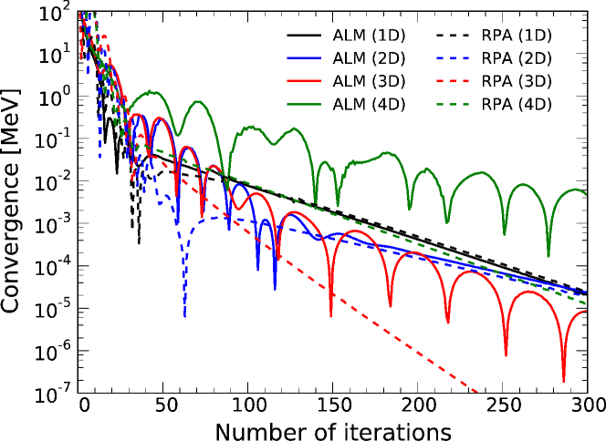
Figure 1: (color online) Convergence of the HFB calculation as function of the number of iterations in ²⁴⁰Pu for four different sets of constraints, see text for details.

2.3.7 Comparison with the Augmented Lagrangian Method

We illustrate in Fig. 1 the performance of the RPA-based method for multiconstraints by comparing it with the ALM, see Section 2.2.2 of [7]. Calculations were all performed in ²⁴⁰Pu for the SkM* functional using a deformed stretched HO basis of 20 shells and deformation $\beta_{2}=0.3$. Four different configurations were considered: (i) a 1D case with only a constraint on $\langle\hat{Q}_{20}\rangle=60$ b, (ii) a 2D case with a constraint on both $\langle\hat{Q}_{20}\rangle=60$ b and $\langle\hat{Q}_{22}\rangle=0$ b, (iii) a 3D case with the constraints $\langle\hat{Q}_{20}\rangle=60$ b, $\langle\hat{Q}_{22}\rangle=0$ b, and $\langle\hat{Q}_{40}\rangle=5$ b², and finally (iv) a 4D case with the constraints $\langle\hat{Q}_{10}\rangle=0$ fm, $\langle\hat{Q}_{20}\rangle=60$ b, $\langle\hat{Q}_{22}\rangle=0$ b, and $\langle\hat{Q}_{30}\rangle=10$ b^3/2. The main advantage of the RPA-based method is that it does take into account correlations between the constraints: while its performance is comparable to the ALM in the 1D and even 2D case, it becomes more and more efficient when the number of constraints increases. Note that the constraints need not be limited to multipole moments: any operator can be included in the list.

2.4 Fission toolkit

Version (v2.73y) of the code hfodd contains a collection of routines employed primarily in fission studies. Among others, they provide

• the capability to impose a constraint on the number of particles in the neck. The Gaussian neck operator is defined as

  $$\hat{Q}_{N}=e^{-(z-z_{N})^{2}/a_{N}^{2}},$$ (88)

  where $z_{N}$ gives the position of the neck (along the $z-$axis of the intrinsic reference frame) between two nascent fragments. It is defined as the point near the origin of the intrinsic reference frame where the density is the lowest. The range $a_{N}$ gives the spatial extent of the neck: in the code, it is fixed at 1 fm.

• the charge, mass, total kinetic, nuclear and pairing energy of each fragment. Expectation values of the multipole moments are also computed, both in the reference frame of the fissioning nucleus and in those of each of the individual fragments.

• the interaction energy between the fragments. Both the nuclear (Skyrme) interaction energy and the direct Coulomb energy are computed. The direct Coulomb energy is a measure of the total kinetic energy of fission fragments.

• the capability to perform a unitary transformation of q.p. operators so as to maximize the spatial localization of each q.p. within a pre-fragment.

All these routines are collected in module hfodd_fission_7.f90 and require (at least) the option IFRAGM=1 set in the input file. Below we give a brief description of each of these features.

2.4.1 Constraint on the size of the neck

The Gaussian neck operator (88) is purely spatial and does not depend on spin or isospin degrees of freedom. Its expectation value is computed in coordinate space on the Gauss-Hermite quadrature grid used in hfodd,

$$\langle\hat{Q}_{N}\rangle=\int d^{3}\bm{r}\hat{Q}_{N}\rho(\bm{r}),$$ (89)

where $\rho(\bm{r})$ is the isoscalar density. The integral is computed by using the quadrature relation

$$\frac{1}{b_{\mu}}\int d\xi_{\mu}f(\xi_{\mu})\;e^{-2\xi_{\mu}^{2}}=\sum_{k_{\mu}}\frac{w_{k_{\mu}}}{b_{\mu}\sqrt{2}}f\left(\frac{\eta_{k_{\mu}}}{\sqrt{2}}\right)$$ (90)

valid for any function $f(x_{\mu})$, with $\xi_{\mu}=b_{\mu}x_{\mu}$ the dimensionless coordinate, $b_{\mu}$ the oscillator length in the direction $\mu$, $\omega_{k_{\mu}}$ and $\eta_{k_{\mu}}$ the weights and nodes of the Gauss-Hermite quadrature. In hfodd, the isoscalar density $\rho(\bm{r})$ is represented by the array DENSIT, which is defined at the points $\eta_{k_{\mu}}/\sqrt{2}$. The function $f$ to integrate for the Gaussian neck operator is, therefore,

$$f(\bm{\xi})=\rho_{0}(\bm{\xi})e^{2\bm{\xi}^{2}}e^{-(\xi_{z}-\xi_{N})^{2}/\alpha_{N}^{2}},$$ (91)

with $\alpha_{N}=b_{z}a_{N}$ and $\xi_{N}=b_{z}z_{N}$.

In order to add a constraint on the expectation value of the neck operator, its matrix elements in the HO basis are also needed. They take the simple form

$$\langle n_{x}n_{y}n_{z}|\hat{Q}_{N}|m_{x}m_{y}m_{z}\rangle=\delta_{n_{x}m_{x}}\delta_{n_{y}m_{y}}I_{n_{z}m_{z}}$$ (92)

with

$$I_{n_{z}m_{z}}=\sum_{k_{z}=0}^{n_{z}+m_{z}}C^{k_{z}}_{n_{z}m_{z}}(00)\int d\xi_{z}\;H_{k_{z}}^{(0)}(\xi_{z})e^{-\xi_{z}^{2}}e^{-\left(\frac{\xi_{z}-\xi_{N}}{\alpha_{N}}\right)^{2}}.$$ (93)

The normalized Hermite polynomials $H_{k_{\mu}}^{(0)}(\xi_{\mu})$ and expansion coefficients $C^{k}_{nm}(00)$ are defined in Section 4.3 of Ref. [1]. One can show that the integral in $I_{n_{z}m_{z}}$ can be computed exactly. Its expression is

$$\int d\xi_{z}\;H_{k_{z}}^{(0)}(\xi_{z})e^{-\xi_{z}^{2}}e^{-\left(\frac{\xi_{z}-\xi_{N}}{\alpha_{N}}\right)^{2}}=\sqrt{\frac{\pi b_{z}a_{N}^{2}}{G_{z}}}e^{-\frac{1}{2}\frac{\alpha_{N}^{2}}{G_{z}}}\frac{1}{G_{z}^{k/2}}\psi_{k_{z}}\left(\frac{\alpha_{N}}{\sqrt{G_{z}}}\right),$$ (94)

with $G_{z}=1+b_{z}^{2}a^{2}_{N}$, and $\psi_{k_{z}}$ is the HO wave-function. From this expression, the matrix elements of $\hat{Q}_{N}$ in the good-simplex basis are easily found using the relations (84) of [1].

2.4.2 Fission fragment properties

The identification of fission fragments is based on the position of the neck and the spatial occupation of quasi-particles. We start from the set of q.p. in the compound nucleus defined by the Bogoliubov matrices $U$ and $V$. We may write the coordinate space representation of the full one-body density matrix (in coordinate$\otimes$spin space) as

$$\rho(\bm{r}\sigma,\bm{r}^{\prime}\sigma^{\prime})=\sum_{\mu}\rho_{\mu}(\bm{r}\sigma,\bm{r}^{\prime}\sigma^{\prime}),$$ (95)

with the q.p. density operator $\rho_{\mu}(\bm{r}\sigma,\bm{r}^{\prime}\sigma^{\prime})$ of q.p. $\mu$ defined (at temperature $T$) by

$$\rho_{\mu}(\bm{r}\sigma,\bm{r}^{\prime}\sigma^{\prime})=\sum_{ij}\left[(1-f_{\mu})V_{i\mu}^{*}V_{j\mu}+f_{\mu}U_{i\mu}U_{j\mu}^{*}\right]\psi_{i}(\bm{r}\sigma)\psi_{j}^{*}(\bm{r}^{\prime}\sigma^{\prime}),$$ (96)

with $\psi_{i}(\bm{r}\sigma)$ the basis functions and $f_{\mu}$ the Fermi-Dirac statistical occupation at temperature $T$. The spatial occupation of the q.p. $\mu$ is then defined as

$$N_{\mu}=\sum_{\sigma}\int d^{3}\bm{r}\;\rho_{\mu}(\bm{r}\sigma,\bm{r}\sigma).$$ (97)

Since the basis $\{\psi_{i}\}$ is orthonormal, this reduces to the expression

$$N_{\mu}=\sum_{ij}\left[(1-f_{\mu})V_{i\mu}^{*}V_{j\mu}+f_{\mu}U_{i\mu}U_{j\mu}^{*}\right],$$ (98)

with the total number of particles defined as $N=\sum_{\mu}N_{\mu}$.

We can then define the occupation of the q.p. $\mu$ in the fragment (1) as

$$N_{1,\mu}=\sum_{ij}\left[(1-f_{\mu})V_{i\mu}^{*}V_{j\mu}+f_{\mu}U_{i\mu}U_{j\mu}^{*}\right]d_{ij}(z),$$ (99)

where

$$d_{ij}(z)=\sum_{\sigma}\int_{-\infty}^{+\infty}dx\int_{-\infty}^{+\infty}dy\int_{-\infty}^{z_{N}}dz\;\psi_{i}(\bm{r}\sigma)\psi_{j}^{*}(\bm{r}\sigma).$$ (100)

The occupation of the q.p. in the fragment (2) is simply $N_{2,\mu}=N_{\mu}-N_{1,\mu}$. We then assign the q.p. $\mu$ to fragment (1) if $N_{1,\mu}\geq 0.5N_{\mu}$, and to fragment (2) if $N_{1,\mu}<0.5N_{\mu}$. This gives us two sets of q.p. with which we can define objects analogs to the density matrix and pairing tensor of each of the fragments.

It was observed that the coordinate representation $\rho_{1}(\bm{r})$ and $\rho_{2}(\bm{r})$ of the densities in a given fragment has a tail that extends significantly into the other fragment [18]. This delocalization of the density can be traced back to the individual quasi-particles, and can be captured by the following indicator

$$\ell_{\mu}=\frac{|N_{1,\mu}-N_{2,\mu}|}{N_{\mu}^{2}},$$ (101)

with $N_{\mu}$ defined by Eq. (98) and $N_{1,\mu},N_{2,\mu}$ by Eq. (99). If $\ell_{\mu}=0$, the q.p. $\mu$ is fully delocalized, if $\ell_{\mu}=1$ it is fully localized either in the left or in the right fragment. The tails in the densities are produced by the contributions from the delocalized q.p. states with relatively large occupation and $0\leq\ell_{\mu}\ll 1$.

2.4.3 Interaction energies

As mentioned above, the identification of a set of q.p. for each fragment fully defines an analog of the density matrix and pairing tensor for each fragment. In coordinate$\otimes$spin space, these objects take the form

$$\rho_{\text{f}}(\bm{r}\sigma,\bm{r}^{\prime}\sigma^{\prime})=\sum_{\mu\in(\text{f})}\sum_{ij}\left[(1-f_{\mu})V_{i\mu}^{*}V_{j\mu}+f_{\mu}U_{i\mu}U_{j\mu}^{*}\right]\;\psi_{i}(\bm{r}\sigma)\psi_{j}^{*}(\bm{r}^{\prime}\sigma^{\prime}),\vskip 6.0pt plus 2.0pt minus 2.0pt$$ (102)

$$\kappa_{\text{f}}(\bm{r}\sigma,\bm{r}^{\prime}\sigma^{\prime})=\sum_{\mu\in(\text{f})}\sum_{ij}\left[(1-f_{\mu})V_{i\mu}^{*}U_{j\mu}+f_{\mu}U_{i\mu}V_{j\mu}^{*}\right]\;\psi_{i}(\bm{r}\sigma)\psi_{j}^{*}(\bm{r}^{\prime}\sigma^{\prime}),$$ (103)

where $\text{f}=1,2$ refers to the fragment. Note that these quantities are not true density operators. In particular, they do not necessarily obey the usual relations $\rho^{2}+\kappa\kappa^{*}=0$. We refer to them as pseudodensities. The diagonal components of the pseudodensities (in coordinate$\otimes$spin space) for each fragment, $\rho_{1}(\bm{r})$, $\rho_{2}(\bm{r})$, $\kappa_{1}(\bm{r})$ and $\kappa_{2}(\bm{r})$, are obtained as usual [19].

From these definitions, fragment energies and interaction energies can be computed in a straightforward manner [20]. The total direct Coulomb interaction energy is computed as

$$E_{\text{Cou}}^{(\text{dir})}=2e^{2}\int d^{3}\bm{r}\int d^{3}\bm{r}^{\prime}\;\frac{\rho_{1}(\bm{r})\rho_{2}(\bm{r}^{\prime})}{|\bm{r}-\bm{r}^{\prime}|},$$ (104)

where $\rho_{f}$ is the proton density in fragment f. In our calculations, this energy was computed using the Green function method as in [1]. The total exchange Coulomb energy is defined as

$$E_{\text{Cou}}^{(\text{dir})}=2e^{2}\int d^{3}\bm{r}\int d^{3}\bm{r}^{\prime}\;\frac{\rho_{1}(\bm{r},\bm{r}^{\prime})\rho_{2}(\bm{r}^{\prime},\bm{r})}{|\bm{r}-\bm{r}^{\prime}|},$$ (105)

In hfodd (v2.73y), the exchange Coulomb energy of each fragment is computed at the Slater approximation, while the Coulomb exchange interaction energy between fragments is computed “exactly” by using an expansion of the Coulomb potential as a sum of Gaussians [6]. The nuclear Skyrme interaction energy is given by

$$E_{\text{int}}^{\text{Skyrme}} =E_{\text{int}}^{1\rightarrow 2}+E_{\text{int}}^{2\rightarrow 1}$$ (106)

$$=\sum_{t=0,1}\int d^{3}\bm{r}\left\{C_{t}^{\rho}\rho_{t}^{(1)}\rho_{t}^{(2)}+C_{t}^{\Delta\rho}\rho_{t}^{(1)}\Delta\rho_{t}^{(2)}\right.$$

$$\qquad+\left.C_{t}^{\tau}\rho_{t}^{(1)}\tau_{t}^{(2)}+C_{t}^{J}\sum_{\mu\nu}J_{\mu\nu,t}^{(1)}J_{\mu\nu,t}^{(2)}+C_{t}^{\nabla J}\rho_{t}^{(1)}\bm{\nabla}\cdot\bm{J}_{t}^{(2)}\right\}$$

$$+\sum_{t=0,1}\int d^{3}\bm{r}\left\{C_{t}^{\rho}\rho_{t}^{(2)}\rho_{t}^{(1)}+C_{t}^{\Delta\rho}\rho_{t}^{(2)}\Delta\rho_{t}^{(1)}\right.$$

$$\qquad+\left.C_{t}^{\tau}\rho_{t}^{(2)}\tau_{t}^{(1)}+C_{t}^{J}\sum_{\mu\nu}J_{\mu\nu,t}^{(2)}J_{\mu\nu,t}^{(1)}+C_{t}^{\nabla J}\rho_{t}^{(2)}\bm{\nabla}\cdot\bm{J}_{t}^{(1)}\right\},$$ (107)

with the traditional densities $\rho$, $\tau$, $\mathbb{J}$ and $\bm{J}$ built from either set (1) or set (2) of q.p. Note that, while some of these terms are symmetric under an exchange $(1)\leftrightarrow(2)$ (terms proportional to $C_{t}^{\rho}$, $C_{t}^{\Delta\rho}$, $C_{t}^{J}$), others are not (those proportional to $C_{t}^{\tau}$ and $C_{t}^{\nabla J}$).

2.4.4 Rotation of Quasiparticles in Fock space

In version (v2.73y), the code hfodd can perform a unitary transformation of the quasiparticles of the HFB solution. In the context of fission, this rotation (in the Fock space) was introduced by Younes and Gogny in Ref. [18] as a method to “localize” the fission fragments. It is the transposition in nuclei of the localization methods introduced long ago in electronic structure theory to describe molecular bonding [18, 20]. We note here that this localization is a different concept than the one discussed recently in terms of the cluster localization [21]. Our unitary transformation is defined by its action on pairs $(\mu,\nu)$ of q.p. states,

$$\begin{array}[]{rclcrcl}U^{\prime}_{\mu}&=&\phantom{-}\cos\theta_{\mu\nu}U_{\mu}+\sin\theta_{\mu\nu}U_{\nu}&,&V^{\prime}_{\mu}&=&\phantom{-}\cos\theta_{\mu\nu}V_{\mu}+\sin\theta_{\mu\nu}V_{\nu},\\ U^{\prime}_{\nu}&=&-\sin\theta_{\mu\nu}U_{\mu}+\cos\theta_{\mu\nu}U_{\nu}&,&V^{\prime}_{\nu}&=&-\sin\theta_{\mu\nu}V_{\mu}+\cos\theta_{\mu\nu}V_{\nu}.\end{array}$$ (108)

Angles of the rotation $\theta_{\mu\nu}$ can be different for every pair of q.p. states. We can, of course, apply a sequence of unitary transformations (108) for arbitrarily selected pairs one after another, and obtain a total unitary transformation that depends on all angles $\theta_{\mu\nu}$. In version (v2.73y), each unitary transformations (108) is chosen so as to maximize the localization (101) in a given pair of q.p. states.

Under transformation (108), the full density matrix of the compound nucleus $\rho$ remains unchanged. However, occupation (98) of a given q.p. $\mu$ becomes

$$N^{\prime}_{\mu}=\sum_{ij}\left[\cos^{2}\theta_{\mu\nu}V^{*}_{i\mu}V_{j\mu}+\sin^{2}\theta_{\mu\nu}V^{*}_{i\nu}V_{j\nu}+\sin\theta_{\mu\nu}\cos\theta_{\mu\nu}(V^{*}_{i\mu}V_{j\nu}+V^{*}_{i\nu}V_{j\mu})\right].$$ (109)

Denoting

$$\omega_{\mu\nu}(z)=\sum_{ij}(V^{*}_{i\mu}V_{j\nu}+V^{*}_{i\nu}V_{j\mu})d_{ij}(z),$$ (110)

we find that the occupations of q.p. $\mu$ in each of the fragment then reads

$$\begin{array}[]{l}\displaystyle N^{\prime}_{1,\mu}=\cos^{2}\theta_{\mu\nu}N_{1,\mu}+\sin^{2}\theta_{\mu\nu}N_{1,\nu}+\sin\theta_{\mu\nu}\cos\theta_{\mu\nu}\;[\omega_{\mu\nu}(-\infty)-\omega_{\mu\nu}(z_{N})],\vskip 6.0pt plus 2.0pt minus 2.0pt\\ \displaystyle N^{\prime}_{2,\mu}=\cos^{2}\theta_{\mu\nu}N_{2,\mu}+\sin^{2}\theta_{\mu\nu}N_{2,\nu}+\sin\theta_{\mu\nu}\cos\theta_{\mu\nu}\;\omega_{\mu\nu}(z_{N}),\end{array}$$ (111)

while for q.p. $\nu$ they are

$$\begin{array}[]{l}\displaystyle N^{\prime}_{1,\nu}=\cos^{2}\theta_{\mu\nu}N_{1,\nu}+\sin^{2}\theta_{\mu\nu}N_{1,\mu}-\sin\theta_{\mu\nu}\cos\theta_{\mu\nu}\;[\omega_{\nu\mu}(-\infty)-\omega_{\nu\mu}(z_{N})],\vskip 6.0pt plus 2.0pt minus 2.0pt\\ \displaystyle N^{\prime}_{2,\nu}=\cos^{2}\theta_{\mu\nu}N_{2,\nu}+\sin^{2}\theta_{\mu\nu}N_{2,\mu}-\sin\theta_{\mu\nu}\cos\theta_{\mu\nu}\;\omega_{\nu\mu}(z_{N}).\end{array}$$ (112)

In the current implementation of the localization method in the code hfodd, the code first searches for all possible pairs $(\mu,\nu)$ such that $|\Delta E|=|E_{\mu}-E_{\nu}|\leq\Delta$, the localization of both q.p. is $\ell_{\mu},\ell_{\nu}\leq\ell_{\mathrm{max}}$ and their occupation is $N_{\mu},N_{\nu}\geq N_{\mathrm{min}}$. The quantities $\Delta$, $\ell_{\mathrm{max}}$, and $N_{\mathrm{min}}$ are user inputs. The localization of q.p. is only performed on those q.p. states that match all these conditions. The code also allows to perform several successive q.p. rotations. Note that, after the first rotation, the HFB matrix is not diagonal anymore: the definition of $\Delta E$ is, therefore, not based on q.p. energies but on the diagonal elements $E_{\mu\mu}$ and $E_{\nu\nu}$ of the rotated HFB matrix.

2.5 Interface with hfbtho

Since version (v2.49t), the code hfodd includes the hfbtho DFT solver as a module. In version (v2.49t), the hfbtho kernel was the one published in [22]. In the current version (v2.73y), we have upgraded the hfbtho kernel to the version 2.00d of [23]. This offers additional capabilities such as the constraints on (axial) multipole moments, the breaking of parity to describe asymmetric nuclear shapes, the finite-temperature HFB theory, etc. In addition to being able to initialize a hfodd calculation with the hfbtho solution, version (v2.73y) also offers the reverse option: the code can read a previous hfodd solution, use it to initialize and run hfbtho before to convert back again to hfodd. Such an option can be useful in axial multi-constrained calculations in heavy nuclei (where hfodd calculations can be time- and resource-consuming) which serve as initial conditions for triaxial calculations. To activate this mode, the user must set IF_THO to 2 in the input file, and must have the hfodd fields recorded on disk.

2.6 Parallel capabilities

Compared to version (v2.49t), several routines have been substantially accelerated through the use of shared memory parallelism with OpenMP. The routines affected are nilasp, nilapn, denmac, spaver, pnaver, gauopt, denshf. In addition, several linear algebra operations such as matrix multiplication or matrix-vector multiplication are now handled by BLAS routines instead of being hard-coded in the program. Since several standard implementations of BLAS and LAPACK are multi-threaded (for instance the Intel MKL or AMD ACML libraries), additional speed-ups can be thus achieved on multicore architectures.

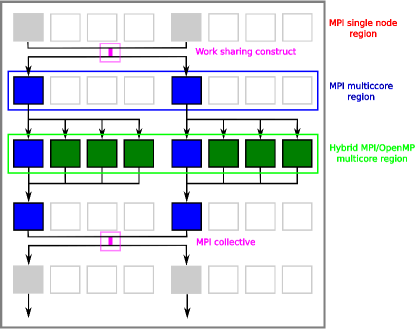
Figure 2: (color online) Schematic representation of the hybrid MPI/OpenMP programming model of hfodd. The figure corresponds to the case where a single HFB calculation is spread across 2 MPI processes, each invoking 4 threads. Light-gray colored boxes show MPI processes working independently of each other; dark blue colored boxes represent MPI processes sharing work; dark green colored boxes show OpenMP threads sharing work of a given MPI process.

In version (v2.73y), the two time-consuming routines denshf and gauopt have also been explicitly parallelized to take advantage of massively parallel architectures (very large node count). As a result, the user can choose to spread one HFB calculation across several MPI processes (typically, between 4 and 8), each MPI process being able to invoke several threads. Note that this option is only available when running in MPI mode and requires specifying at compile time the number of MPI processes handling a given hfodd calculation; see section 4.2 for details. In such a case, the program handles three different levels of parallelism for:

Level 1 Number of HFB calculations $N$;

Level 2 Number of MPI processes involved in each HFB calculation $N_{\mathrm{p}}$;

Level 3 Number of OpenMP threads called in each MPI process $N_{\mathrm{t}}$.

The total number of cores required in such a calculation is thus $N_{\mathrm{cores}}=N\times N_{\mathrm{p}}\times N_{\mathrm{t}}$. Internally, the program splits MPI_COMM_WORLD into three sets of communicators: one corresponding to each group of processes handling a HFB calculation; one including all the master processors across all groups; the last one including all the slaves across all groups. MPI collective operations can then be easily defined within a given group. Note that the ratio (time of calculation)/(time of communication) remains very large so that load imbalance issues are negligible at this stage.

Figure 2 schematically illustrates the workflow of a single HFB calculation in this case. Most of the code execution is serial: all MPI processes involved perform exactly the same task. When the code enters a parallelized segment of the code, work is shared explicitly across available MPI processes. In both routines, the parallel segment involves nested loops: each MPI process handles different values of the index of the outermost loop. Some time within the parallel region, each MPI task may enter a multi-threaded region (OpenMP). At the end of the MPI parallel region, results from each MPI process are combined and broadcast back to each MPI process. This step involves blocking collective MPI operations.

In denshf, the outermost loop involves the node index $k_{z}$ of the Gauss-Hermite mesh in the $z$ direction. Each MPI process computes different $k_{z}$ values in parallel, hence a sub-array of the full density array. For example, with 2 MPI tasks, process 0 would compute all densities at all even values of $k_{z}$, while process 1 would compute all odd values. At the end, a call to mpi_allgatherv gathers these different subarrays into the full density array. In gauopt, the outermost loop involves a summation over the quantum number $n_{x}$. Each MPI process thus performs a partial summation over a subset of $n_{x}$ values, and the collective MPI operation at the end of the routine is thus a call to mpi_allreduce, which sums all contributions from the different MPI processes.

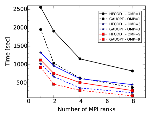
Figure 3: (color online) Scaling of execution time for 10 iterations of the Gogny force as a function of the number of MPI processes per HFB calculation and the number of OpenMP threads. Curves with plain lines correspond to the full HFODD execution time, curves with dashed lines for the time spent in the routine GAUOPT; see text for details.

Figure 3 shows the speed-up achieved by parallelizing the kernel of a HFB calculation in the case of the Gogny force. Calculations were performed in a full spherical basis of 14 major oscillator shells and the number of Gauss-Hermite points was set to 30 in each Cartesian direction. The full two-body center of mass correction was included. Results can be reproduced by using the file sn120_gogny.dat included with the code and increasing the size of the basis accordingly. With the current implementation, execution time can be reduced by a factor 8.5 between a pure serial mode and a hybrid MPI-OpenMP mode with 8 MPI ranks and 9 OpenMP threads; a speed-up of 3 can be achieved between serial and non-threaded MPI mode.

2.7 Lipkin translational energy

The Lipkin method was proposed in the early nineteen sixties to approximately restore broken symmetries at the mean-field level by adding terms in the functional that cancel out the effects of quantum fluctuations on the total energy [24]. The method requires defining the Lipkin operator to add to the two-body effective Hamiltonian [25, 7]. In the case of the translational-symmetry restoration, the Lipkin operator reads

$$\hat{K}=\sum_{i=x,y,z}k_{i}\hat{P}_{i}^{2}$$ (113)

where $\hat{P}_{i}$ is the total linear momentum in the direction $i$, and $k_{i}$ is a parameter weighting the dependence of $\hat{P}_{i}^{2}$ in the energy. In version (2.49t), all parameters $k_{i}$ were forced to be equal, and the correction could not be computed in the presence of pairing correlations (BCS or HFB). In version (v2.73y), these restrictions have been removed. Note that different values of $k_{i}$ allow us to treat differences of the linear-momentum fluctuations along the three principal axes of a deformed nucleus.

The expectation value of $\hat{P}_{i}^{2}$ in the HFB ground-state reads

$$\langle\hat{P}_{i}^{2}\rangle=\left[{\mathrm{T}r}\left(P_{i}\rho\right)\right]^{2}+{\mathrm{T}r}\left[P_{i}^{2}\rho\right]-{\mathrm{T}r}\left[P_{i}\rho P_{i}\rho\right]-{\mathrm{T}r}\left[P_{i}\kappa\left(P_{i}\kappa\right)^{*}\right]$$ (114)

where $P_{i}$ is the matrix of $\hat{P}_{i}$ in the good-simplex basis of hfodd, $\rho$ is the one-body density matrix, and $\kappa$ is the pairing tensor. The last term is non-zero only when pairing is active.

Since operator $\hat{P}_{i}^{2}$ does not break time-reversal, simplex, parity, or T-simplex symmetries (see [4] for a definition of these symmetries), the code can maintain them during the calculation except when determining parameters $k_{i}$ by shifting wave functions. This is because the shifted wave functions may lose some of the symmetries. For example, after a shift along the $y$ axis, the wave function no longer conserves the simplex.

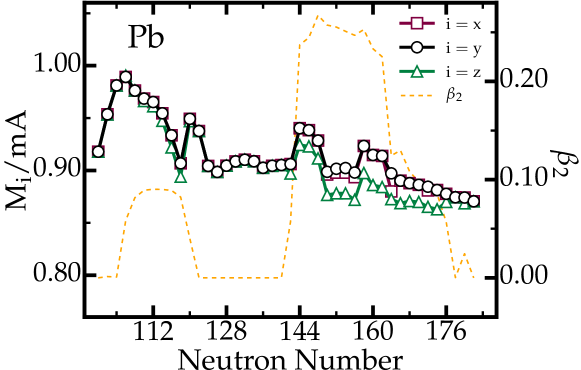
Figure 4: Ratios $M_{i}/mA$ between the renormalized (along $i=x$, $y$ or $z$ axis) and exact masses for the Pb isotopic chain after Lipkin minimization. For reference, the $\beta_{2}$ axial quadrupole deformation is also plotted.

When pairing is active, the determination procedure of parameters $k_{i}$ is still the same as that outlined in Ref. [25]. By shifting wave functions in the $i$th direction by $R_{i}$, $\left|\Phi\left(R_{i}\right)\right\rangle=\text{$\exp$}\left(i\hat{P}_{i}R_{i}\right)\left|\Phi\right\rangle$, and calculating overlaps and matrix elements, respectively, $\left\langle\Phi\right|\hat{H}\left|\Phi\left(R_{i}\right)\right\rangle$ and $\left\langle\Phi\right|\hat{P}_{i}^{2}\left|\Phi\left(R_{i}\right)\right\rangle$, one reaches a new point on the $E=E\left(\langle P_{i}^{2}\rangle\right)$ curve and then one can extract the slope in direction $i$, which is just $k_{i}$.

Calculation of the parameters $k_{i}$ can also be performed using the Gaussian overlap approximation [7]. In the case with pairing, overlaps $\left\langle\Phi|\Phi(R_{i})\right\rangle$ are calculated using the Pfaffian techniques [26, 27].

Fig. 4 shows ratios of the renormalized and exact masses for the Pb isotope chain. Calculations were performed in the space of $N_{0}=16$ HO shells and with the SLy4 parametrization of the Skyrme EDF. A volume zero-range pairing interaction with a cutoff window of $E_{\mathrm{cut}}=60$ MeV was used with the pairing strengths of $V_{n}=-159$ and $V_{p}=-152$ MeV fm³ for neutrons and protons, respectively. The renormalized mass is defined as $M_{i}=1/2k_{i}$. As one can see, if the nucleus is deformed, renormalized masses in different directions are not equal. Note that even small differences in masses can have a large impact on the total energy, especially in heavy nuclei.

2.8 Higher-order Lipkin particle-number corrections

Version (v2.73y) of the code hfodd allows for the treatment of Lipkin particle-number corrections to higher orders [28]. The Lipkin method [24] was proposed as a computationally inexpensive way to obtain an approximate variation-after-particle energy. For the case of the variation after particle-number projection (VAPNP), it is realized through an auxiliary Routhian,

$$\hat{H}^{\prime}=\hat{H}-\hat{K}[\hat{N}-N_{0}]\,,$$ (115)

where the Lipkin operator $\hat{K}$ is a function of the shifted particle-number operator $\hat{N}-N_{0}$. The role of the Lipkin operator $\hat{K}$ is to “flatten" the average Routhian as a function of the particle number [24, 25, 28], that is, to make it independent of the particle-number fluctuations. As there exists no such an exact operator, assumptions for the Lipkin operator $\hat{K}$ have to be made. As proposed by Lipkin [24], the simplest and manageable ansatz is in the form of a polynomial,

$$\hat{K}[\hat{N}-N_{0}]=\sum_{m=1}^{M}k_{m}(\hat{N}-N_{0})^{m}\,,$$ (116)

where $k_{1}\equiv\lambda$ is the Fermi energy, which is used as a Lagrange multiplier to fix the average particle number. The higher-order Lipkin parameters $k_{m}$ for $m>1$, which are used to best describe the particle-number dependence of the average energies of projected states, can no longer be regarded as Lagrange multipliers, but they are determined as follows.

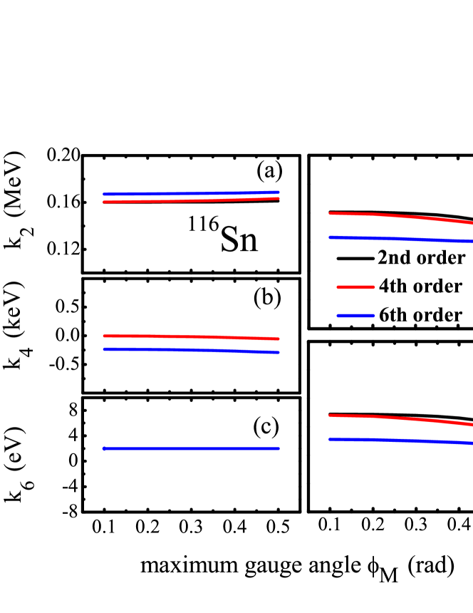
Figure 5: The Lipkin parameters $k_{2}$ (a), $k_{4}$ (b), and $k_{6}$ (c), Lipkin correction energy $E_{\text{corr}}=-\sum_{m=1}^{M}k_{m}n_{m}(0)$ (d), and Lipkin VAPNP energy $E_{N_{0}}=\langle\Phi|\hat{H}-\hat{K}[\hat{N}-N_{0}]|\Phi\rangle$ (e), determined for neutrons in ¹¹⁶Sn at second, fourth, and sixth orders, as functions of the maximum gauge angle $\phi_{M}$. The Lipkin parameters $k_{2}$, $k_{4}$, and $k_{6}$ are in units of MeV, keV, and eV, respectively, illustrating the rapid convergence of the power expansions. The particle-hole channel was described with the SIII parametrization of the Skyrme EDF [29], and the particle-particle channel by a volume pairing force with strength $V_{0}=-155.45$ MeV. The proton pairing was switched off.

We begin by defining the HFB wave functions shifted in the gauge space as $|\Phi(\phi)\rangle=\exp\left(i\phi(\hat{N}-N_{0})\right)|\Phi\rangle$, which gives us the overlap, energy, and particle-number kernels $I(\phi)=\langle\Phi|\Phi(\phi)\rangle$, $H(\phi)=\langle\Phi|\hat{H}|\Phi(\phi)\rangle$, and $N_{m}(\phi)=\langle\Phi|(\hat{N}-N_{0})^{m}|\Phi(\phi)\rangle$, respectively. Then, Eqs. (115) and (116) combine to

$$h^{\prime}(\phi)=h(\phi)-\sum_{m=1}^{M}k_{m}n_{m}(\phi)\,,$$ (117)

where the reduced kernels are

$$h^{\prime}(\phi)=\frac{H^{\prime}(\phi)}{I(\phi)}\,,~{}h(\phi)=\frac{H(\phi)}{I(\phi)}\,,~{}n_{m}(\phi)=\frac{N_{m}(\phi)}{I(\phi)}\,.$$ (118)

Assuming that the reduced Routhian kernel $h^{\prime}(\phi)$ is perfectly flat, that is, $h^{\prime}(\phi)\equiv{C}$ for all $\phi$, the Lipkin parameters $k_{m}$ for $m=1,\ldots,M$ can be determined from

$$C+\sum_{m}k_{m}n_{m}(\phi_{i})=h(\phi_{i})\,.$$ (119)

This equation is assumed to hold at gauge angle $\phi=\phi_{0}=0$ and also at $M$ other nonzero values of the gauge angle $\phi_{i}$, which gives a set of linear equations for $k_{m}$. In practice, equally spaced values of $\phi_{i}=i\phi_{1}$ can be used [28], which gives the maximum gauge angle $\phi_{M}=M\phi_{1}$. At convergence of the expansion of the Lipkin operator (116), the resulting Lipkin parameters should not depend on the maximum gauge angle.

When calculating the projected energies, the largest contributions to the integrals in the gauge space come from the vicinity of the origin due to the largest weight [30]. The singularities caused by the vanishing overlaps have quite small influences on the reduced kernels near the origin [31]. Therefore, we evaluate Lipkin parameters $k_{m}$ using the gauge-shifted HFB states not far away from the origin, that is, the value of the maximum gauge angle (the largest gauge angle chosen for the determinations of Lipkin parameters) should be small.

In Fig. 5, we show an example of the Lipkin parameters calculated for the neutron states in ¹¹⁶Sn. The results for the second, fourth, and sixth orders ar shown as functions of the maximum gauge angle $\phi_{M}$. For ¹¹⁶Sn, which is a typical mid-shell nucleus, the dependence of the Lipkin parameter on $\phi_{M}$ is weak already at second order, and thus higher-order Lipkin method does not give much of an improvement, see Ref. [28] for the full discussion.

2.9 Interface to a plotting program

The hfodd review file FILREV, see Section II-3.9 [2], is a plain-text file that can be used to extract information necessary for creating various kinds of plots. As an example, the present distribution (v2.73y) contains script getLevels.py, which reads the hfodd review file and prepares data files that can be used to plot single-particle energies or Routhians as functions of deformation ($Q_{20}$ moment) or rotational frequency ($\omega$).

In order to use the script, one has to run hfodd for a series of deformations/frequencies, corresponding to different values of QASKED (under the keyword MULTCONSTR in the hfodd input file) or OMEGAY (under keyword OMEGAY or OMEGA_XYZ). It should be remembered, however, that multipole moment $q_{20}$ of a converged solution may not be exactly equal to QASKED — discrepancies can be quite large, but, at least to some extend, can be controlled by adjusting stiffness parameter (STIFFQ under keyword MULTCONSTR in the hfodd’s input data file). Alternatively, one can use the ALM, see Section VI-2.2.2 [6]. Of course, the hfodd review file has to contain data describing single-particle levels, which means the parameter IREVIE (under the keyword REVIEW in the hfodd input file) must be set to at least 2.

In the present distribution (v2.73y), two examples of hfodd review files are provided: DyDef.rev corresponds to a series of deformations and DyOme.rev to a series of rotational frequencies. These two review files were obtained by running the code hfodd on input data files DyDef.dat and DyOme.dat, respectively.

Having a hfodd review file prepared, one can run the script getLevels.py with three or four arguments:

• The first (required) argument is the name of the hfodd review file produced by running the code hfodd – it should correspond to a series of results obtained from runs of the code hfodd with input data differing by the value of deformation (QASKED) or rotational frequency (OMEGAY or OMEGAX or OMEGAZ). Such a file can also be merged “by hand” from several files created in separate runs.

• The second (required) argument specifies the quantity which plays the role of the independent variable:
        ’d’ (or ’D’, or ’q’, or ’Q’) — deformation (q20);
        ’f’ (or ’F’, or ’o’, or ’O’) — rotational frequency ($\omega$); by default $\omega_{y}$ is understood, but adding letter ’x’ or ’y’ or ’z’ (e.g., ’fy’ or ’oz’) another component may be selected

• The third (required) argument is:
        ’N’ (or ’n’) — neutrons,
        ’Z’ (or ’z’, or ’P’, or ’p’) — protons.

• The fourth (optional) argument determines the name of the output file; if it is name, then the output file will be name_XXX_Y.lev, where XXX is def for curves vs. deformation ($q_{20}$) and omQ for curves vs. rotational frequency, with ’Q’ equal to ’x’, ’y’ or ’z’, while Y is N for neutrons and Z for protons. If not specified, name defaults to the name of the input file with its extension .rev stripped off.

For example, with the two review files mentioned above, one can run

            ./getLevels.py DyDef.rev d n
            ./getLevels.py DyDef.rev d z
            ./getLevels.py DyOme.rev f n
            ./getLevels.py DyOme.rev f z

to get files DyDef_def_N.lev, DyDef_def_Z.lev, DyOme_omy_N.lev, and DyOme_omy_Z.lev, respectively.

The output file of the script is a pure text file and has the following format:

• The first ten lines constitute a header containing some metadata about the current run; they look like this

          # Created on  : 2016-07-21 23:38:22.843367
          # Version     : 1.1
          # Run by      : <user name>
          # Input file  : DyDef.rev
          # Output file : DyDef_def_N.lev
          # N and Z     : 86 66
          # Levels for  : neutrons
          # Curves vs.  : 10 deformations (q20)
          # Phony ene   : 16.0 MeV
          # No of curves: 111
          
  

  For curves in function of frequency, the name of the output file will contain omy instead of def (line 5) and omegas instead of deformations (line 8).

• After the header, information on all extracted curves is written one after another. The number of curves is specified in the last line of the header. Data corresponding to each curve are preceded by exactly one blank line. A segment of data describing one curve has the following two forms:

  • In the case of single-particle energies as functions of deformation:

                    #  3/2 +1 7
                    -11.469401879 -2.0959741301 |4,1,1,3/2>
                    1.724126373 -3.8251360412 |6,3,1,3/2>
                    7.4711027963 -5.8204478799 |6,5,1,3/2>
                    9.6541267607 -6.684000508 |6,5,1,3/2>
                    13.883562273 -7.8581971 |6,5,1,3/2>
                    23.059344121 -9.0080832634 |4,0,2,3/2>
                    39.292223291 -5.9512624571 |4,0,2,3/2>
                    41.950864161 -5.3978081111 |4,0,2,3/2>
                    44.87486028 -5.7117002799 |6,4,2,3/2>
                    48.23253362 -6.5226929621 |6,4,2,3/2>
                    
    

    where the three elements in the first, comment line denote $j_{z}$, parity and curve number (starting from 1 for the lowest state with given $j_{z}$ and parity). Each point of the curve is then represented by three space-separated elements: deformation ($q_{20}$), energy, and the Nilsson label of the leading component of a given state (the label will not contain any embedded spaces.) Note that the label does not have to be the same for all points along a single curve.

  • In the case of Routhians as functions of the rotational frequency:

                    # -1 +1 23
                    0.001 -7.3419171589 |5,2,1,3/2>
                    0.1 -7.3449823643 |5,2,1,3/2>
                    0.2 -7.3563104158 |5,2,1,3/2>
                    0.3 -7.3826283035 |5,2,1,3/2>
                    0.4 -7.4347954666 |5,2,1,3/2>
                    0.5 -7.5198781158 |5,2,1,3/2>
                    0.6 -7.634943286 |5,2,1,3/2>
                    0.7 -7.76903774 |5,2,1,3/2>
                    0.8 -7.9093199047 |5,2,1,3/2>
                    
    

    the form is similar, but the comment line specifies parity, signature and the curve number. The first number on each line now denotes the rotational frequency.

It may happen that states which belong to a given orbital are present at some deformations (frequencies) but are missing at other deformations, as they were too high to be calculated and/or output by hfodd. In this situation, the script adds “artificial” points to the curve with all quantum numbers in the Nilsson label set to zero and energy set to phonyEne. The value of phonyEne can be found in the ninth line of the header and is guaranteed to be larger by at least 2MeV than the largest “true” energy present in the data. Additionally, an asterisk is added at the end of lines corresponding to these “artifical” points. For example, for data in file DyDef_def_N.lev, the value of phonyEne is 16 MeV, and one of the orbital is written as

                #  1/2 -1 11
                -29.988366225 16.0 |0,0,0,0/2> *
                -19.994324961 7.0230247553 |5,4,1,1/2>
                -8.59922993 -0.79098160199 |5,4,1,1/2>
                0.54349578927 -2.3664542895 |5,3,0,1/2>
                10.031225775 -4.0948376775 |5,1,0,1/2>
                21.183531098 -2.7050254605 |7,7,0,1/2>
                30.131724613 -6.1232544454 |7,7,0,1/2>
                40.0 -5.758469044 |5,2,1,1/2>
                50.000000013 -7.0317367018 |7,6,1,1/2>
                60.143378687 -8.1834216685 |7,6,1,1/2>
                

2.10 Strong-force isospin-symmetry-breaking terms

It is well known that mean-field models involving isospin-invariant strong force and the Coulomb interaction constituting the only source of the ISB fail to reproduce both mirror displacement energies (MDEs) [32] and triplet displacement energies (TDEs) [33]. These primary indicators of the ISB effects are defined as

$$\mathrm{MDE} = \mathrm{BE}\left(T,T_{3}=-T\right)-\mathrm{BE}\left(T,T_{3}=+T\right),$$ (120)

$$\mathrm{TDE} = \mathrm{BE}\left(T=1,T_{3}=-1\right)+\mathrm{BE}\left(T=1,T_{3}=+1\right)-2\mathrm{BE}\left(T=1,T_{3}=0\right),$$ (121)

where $\mathrm{BE}(T,T_{3})$ denotes the binding energy of a nucleus with total isospin $T$ and its projection $T_{3}$. To account quantitatively for the MDEs and TDEs, mean-field models must be extended by including charge dependent components originating from the strong force.

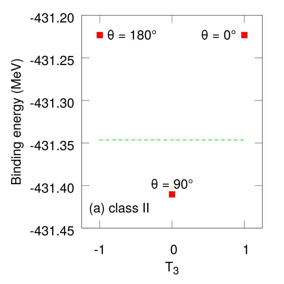
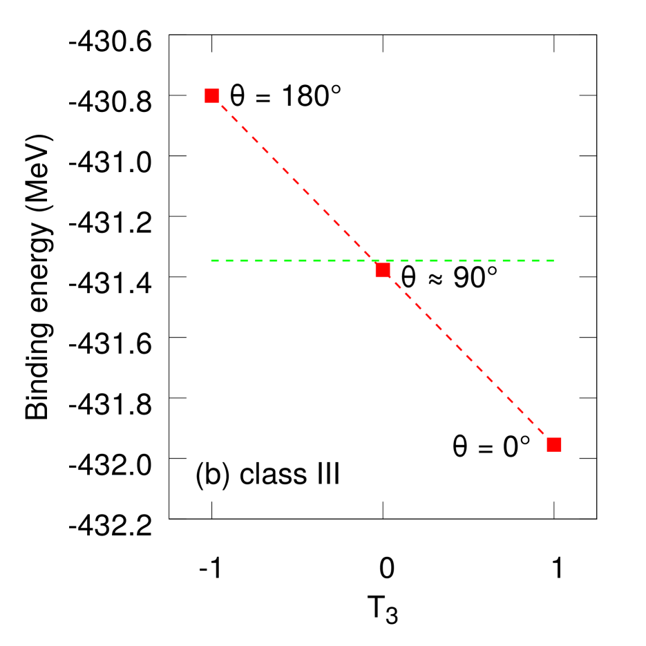
Figure 6: Ground-state energies in the $A=42$ isobaric-triplet nuclei. Calculations were performed without the Coulomb interaction. Panel (a) shows the result obtained using the class II force only with $t_{0}^{\mathrm{II}}=+20$ MeV fm³; Panel (b) shows the result obtained using the class III force only with $t_{0}^{\mathrm{III}}=-8$ MeV fm³. In both panels, the horizontal dashed line shows the ground-state energy obtained using charge-independent model. The slanted dashed line in panel (b) indicates an almost exact linear trend in the calculated masses.

Table 3: Ground-state energies in the $A=42$ isobaric-triplet nuclei. Results obtained without and with the Coulomb interaction are shown in the second and the third column, respectively. The energies, MDEs and TDEs are given in MeV. The first column gives values of the coupling constants $t^{\mathrm{II}}_{0}$ and $t^{\mathrm{III}}_{0}$ in MeV fm³.

		Without Coulomb					With Coulomb
		$\theta$ [∘]	$T_{3}$	Energy	MDE	TDE	$\theta$ [∘]	$T_{3}$	Energy	MDE	TDE
$\scriptstyle t_{0}^{\mathrm{II}}=\;0.0$ $\scriptstyle t^{\mathrm{III}}_{0}=\;0.0$		0.0	1	$-$431.346	0.000	0.000	0.0	1	$-$358.274	13.789	0.159
		90.0	0	$-$431.346			88.9	0	$-$351.459
		180.0	$-$1	$-$431.346			180.0	$-$1	$-$344.485
$\scriptstyle t^{\mathrm{II}}_{0}=\;20.0$ $\scriptstyle t^{\mathrm{III}}_{0}=\;0.0$		0.0	1	$-$431.223	0.000	0.374	0.0	1	$-$358.141	13.783	0.525
		90.0	0	$-$431.410			88.9	0	$-$351.512
		180.0	$-$1	$-$431.223			180.0	$-$1	$-$344.358
$\scriptstyle t_{0}^{\mathrm{II}}=\;0.0$ $\scriptstyle t^{\mathrm{III}}_{0}=\,-8.0$		0.0	1	$-$431.955	1.153	$-$0.002	0.0	1	$-$359.038	14.899	0.145
		95.5	0	$-$431.377			94.0	0	$-$351.661
		180.0	$-$1	$-$430.801			180.0	$-$1	$-$344.139
$\scriptstyle t_{0}^{\mathrm{II}}=\;20.0$ $\scriptstyle t^{\mathrm{III}}_{0}=\,-8.0$		0.0	1	$-$431.827	1.147	0.372	0.0	1	$-$358.894	14.888	0.511
		95.5	0	$-$431.440			94.0	0	$-$351.706
		180.0	$-$1	$-$430.680			180.0	$-$1	$-$344.007

In version (v2.73y), the strong-force ISB terms were added as effective, two-body, zero-range corrections to the conventional isospin-invariant Skyrme interaction. Contributions of class II and class III forces (according to the classification of Henley and Miller [34]) were implemented as follows

$$\hat{V}^{\textit{II}}(i,j) = \frac{1}{2}t^{\mathrm{II}}_{0}\,\delta\left(\bm{r}_{i}-\bm{r}_{j}\right)\left(1-x^{\mathrm{II}}_{0}\,\hat{P}^{\sigma}_{ij}\right)\left[3\hat{\tau}_{3}(i)\hat{\tau}_{3}(j)-\vec{\tau}(i)\circ\vec{\tau}(j)\right],$$ (122)

$$\hat{V}^{\textit{III}}(i,j) = \frac{1}{2}t^{\mathrm{III}}_{0}\,\delta\left(\bm{r}_{i}-\bm{r}_{j}\right)\left(1-x^{\mathrm{III}}_{0}\,\hat{P}^{\sigma}_{ij}\right)\left[\hat{\tau}_{3}(i)+\hat{\tau}_{3}(j)\right],$$ (123)

where $i$, $j$ label nucleons, $t_{0}^{\mathrm{II}}$, $x_{0}^{\mathrm{II}}$, $t_{0}^{\mathrm{III}}$, and $x_{0}^{\mathrm{III}}$ are coupling constants, $\hat{P}^{\sigma}_{ij}$ is the usual spin-exchange operator, and $\vec{\tau}\equiv(\hat{\tau}_{1},\hat{\tau}_{2},\hat{\tau}_{3})$ are the isospin Pauli matrices. Both forces are charge dependent, but only class III breaks charge symmetry. The corresponding energy densities read

$$\mathcal{H}^{\textit{II}} = \frac{1}{2}t^{\mathrm{II}}_{0}\left(1-x^{\mathrm{II}}_{0}\right)\left(\rho_{n}^{2}+\rho_{p}^{2}-2\rho_{n}\rho_{p}-2\rho_{np}\rho_{pn}-\bm{s}_{n}^{2}-\bm{s}_{p}^{2}+2\bm{s}_{n}\cdot\bm{s}_{p}+2\bm{s}_{np}\cdot\bm{s}_{pn}\right),$$ (124)

$$\mathcal{H}^{\textit{III}} = \frac{1}{2}t^{\mathrm{III}}_{0}\left(1-x^{\mathrm{III}}_{0}\right)\left(\rho_{n}^{2}-\rho_{p}^{2}-\bm{s}_{n}^{2}+\bm{s}_{p}^{2}\right),$$ (125)

and the contributions to the mean-field potentials of Ref. [9] are:

$$\begin{array}[]{rcl}U^{\textit{II}}_{n}&=&t^{\mathrm{II}}_{0}\left(1-x^{\mathrm{II}}_{0}\right)\left(+\rho_{n}-\rho_{p}\right),\\[4.30554pt] U^{\textit{II}}_{p}&=&t^{\mathrm{II}}_{0}\left(1-x^{\mathrm{II}}_{0}\right)\left(-\rho_{n}+\rho_{p}\right),\\[4.30554pt] U^{\textit{II}}_{np}&=&t^{\mathrm{II}}_{0}\left(1-x^{\mathrm{II}}_{0}\right)\left(-\rho_{np}\right),\\[4.30554pt] U^{\textit{III}}_{n}&=&t^{\mathrm{III}}_{0}\left(1-x^{\mathrm{III}}_{0}\right)\left(+\rho_{n}\right),\\[4.30554pt] U^{\textit{III}}_{p}&=&t^{\mathrm{III}}_{0}\left(1-x^{\mathrm{III}}_{0}\right)\left(-\rho_{p}\right),\end{array}\hskip 56.9055pt\begin{array}[]{rcl}\bm{\Sigma}^{\textit{II}}_{n}&=&t^{\mathrm{II}}_{0}\left(1-x^{\mathrm{II}}_{0}\right)\left(-\bm{s}_{n}+\bm{s}_{p}\right),\\[4.30554pt] \bm{\Sigma}^{\textit{II}}_{p}&=&t^{\mathrm{II}}_{0}\left(1-x^{\mathrm{II}}_{0}\right)\left(+\bm{s}_{n}-\bm{s}_{p}\right),\\[4.30554pt] \bm{\Sigma}^{\textit{II}}_{np}&=&t^{\mathrm{II}}_{0}\left(1-x^{\mathrm{II}}_{0}\right)\left(+\bm{s}_{np}\right),\\[4.30554pt] \bm{\Sigma}^{\textit{III}}_{n}&=&t^{\mathrm{III}}_{0}\left(1-x^{\mathrm{III}}_{0}\right)\left(-\bm{s}_{n}\right),\\[4.30554pt] \bm{\Sigma}^{\textit{III}}_{p}&=&t^{\mathrm{III}}_{0}\left(1-x^{\mathrm{III}}_{0}\right)\left(+\bm{s}_{p}\right).\end{array}$$ (126)

The formulas above indicate that the parameters $x^{\mathrm{II}}_{0}$ and $x^{\mathrm{III}}_{0}$ are redundant and can be set to zero what we do hereafter. However, to maintain compatibility with future implementations of the finite-range ISB interactions, parameters $x^{\mathrm{II}}_{0}$ and $x^{\mathrm{III}}_{0}$ can still be specified explicitely in the input file, see Sect. 3.1.1.

Note that the contributions due to class II forces depend explicitly on the p-n-mixed scalar and vector densities $\rho_{np}$ and $\bm{s}_{np}$, respectively. Therefore, such forces can only be used within the mean-field formalism involving p-n mixing, whereas calculations with class III forces, which only depend on the standard isoscalar densities, do not require p-n mixing. For the sake of consistency, however, all numerical results shown in this Section have been obtained in the framework involving p-n mixing developed in Ref. [11] and described in detail in Sect. 2.1. Note also, that the spin density $\bm{s}$ is non-zero only when time-reversal symmetry is internally broken, which is the case for the odd and odd-odd nuclei.

To verify the influence of the new terms on the HF ground-state solutions, we have performed test calculations without the Coulomb interaction. This simplification allows for direct testing of the ISB effects caused separately by class II and class III terms. Fig. 6(a) shows the effect of class II force on the ground-state energies in the isospin triplet. As anticipated, the class II interaction is responsible for the curvature of the binding energies of the triplet. Indeed, in this case the $T_{3}=\pm 1$ nuclei are shifted up in the energy by the same value whereas the $T_{3}=0$ nucleus is shifted down (cf. Table 3). Results obtained with class III force are shown in Fig. 6(b). In this case the $T_{3}=0$ nucleus is almost unaffected, whereas the $T_{3}=\pm 1$ nuclei are shifted in opposite directions by nearly the same energy (cf. Table 3). These results confirm that the class II (III) forces modify the TDE (MDE) essentially not influencing the MDE (TDE), respectively.

Table 3 shows the calculated MDE and TDE for a representative example of the $A=42$ triplet using different variants of the model. By comparing the calculated values to the experimental data MDE${}_{exp}=15.007$ MeV and TDE${}_{exp}=0.590$ MeV one immediately concludes that the Coulomb interaction alone is indeed not sufficient to reproduce the data. Taking into account the ISB strong components clearly improves the agreement between theory and experiment. More systematic preliminary study performed in Ref. [35] shows that the class II and III terms implemented here allow to reproduce quite well experimental data on MDE and TDE in a wide range of masses.

2.11 Augmented Lagrangian Method for calculations with 3D constraints on angular momentum and isospin

Following the previous implementation in the hfodd code of the ALM for multipole moments, see Section VI-2.2.2, in version (v2.73y) we implemented the same methodology for constraints on angular momentum and isospin. To this effect, we added to the total energy ${\cal E}$ the ALM constraints as

$${\cal E}^{\prime}={\cal E}-\sum_{\mu=x,y,z}\omega_{\mu}\left(\langle\hat{J}_{\mu}\rangle-\bar{J}_{\mu}\right)+\sum_{\mu=x,y,z}C_{\mu}\left(\langle\hat{J}_{\mu}\rangle-\bar{J}_{\mu}\right)^{2}-\sum_{k=1,2,3}\lambda_{k}\left(\langle\hat{t}_{k}\rangle-\bar{t}_{k}\right)+\sum_{k=1,2,3}C_{k}\left(\langle\hat{t}_{k}\rangle-\bar{t}_{k}\right)^{2}.$$ (127)

In fact, the constraints on the angular momentum were already implemented in version (2.08i), see Section VI-2.3 [6], so the ALM only required introducing corrective terms $\delta\omega_{\mu}$, and updating the angular frequencies as $\omega_{\mu}=\omega^{0}_{\mu}+\delta\omega_{\mu}$, with $\omega^{0}_{\mu}$ denoting the previous fixed values. A similar technology was used for the constraints on the isospin, whereby the previous fixed values of the isocranking frequencies $\lambda^{0}_{k}$, see Section 2.1, were updated as $\lambda_{k}=\lambda^{0}_{k}+\delta\lambda_{k}$.

2.12 Corrected errors

In the present version (v2.73y), we have corrected the following errors of the previous published version (v2.49t) [7].

2.12.1 Entropy

The entropy calculated in version (v2.49t) was too small by a factor two. As a consequence, the Maxwell relations of thermodynamics could not be satisfied.

2.12.2 Finite Temperature BCS Calculations

In the extension of the Hartree-Fock with BCS pairing correlations at finite temperature, the spectral gap is defined by

$$\Delta=\frac{\sum_{n}u_{n}v_{n}\Delta_{n}}{\sum_{n}{u_{n}v_{n}}},$$ (128)

where $u_{n}$ and $v_{n}$ are the usual BCS occupations of single-particle states. When temperature increases, pairing correlations vanish and the denominator of this expression can become zero. In version (v2.49t), the value of the denominator was not tested, which could lead to undefined values.

2.12.3 Symmetries

When calculating contributions to the mean field from the finite-range Coulomb (exchange), Yukawa, or Gogny interactions, the densities are computed directly in the configuration space $\rho_{ij}$ (that is, on the HO basis), which involves the whole $\mathbb{R}^{3}$ domain, irrespective of symmetries of the problem. Conversely, the Skyrme-type mean fields, including the density-dependent terms, are expressed as functions of densities. Therefore, they are computed in the coordinate-space representation $\rho(\bm{r})$, and thus are explicitly symmetrized, so as to benefit from symmetries of the problem. When both types of mean fields are simultaneously present, this may create an inconsistency between the two contributions. In version (v2.49t), in the case of the Gogny force, the resulting small numerical inconsistency was building up along the self-consistent iterations and led to divergences. Enforcing the calculation of unsymmetrized coordinate-space densities resolved the problem.

2.12.4 Skyrme parameters

The Skyrme-force parameter sets predefined for acronyms SLY4, SLY5, SLY7 and sly4, sly5, sly7 were coded in an opposite way with respect to what was presented in Section VI-2.4.2 [6]. Moreover, parameter sets predefined for acronyms SLY6 and SLY7 were incorrectly accompanied by the switch IETACM=1 (two-body center-of-mass correction after variation), whereas these forces have been fitted with the center-of-mass correction before variation, and should have been accompanied the switch IETACM=2. In addition, for acronym UDF0, the values predefined for the Skyrme force UNEDF0 corresponded to preliminary results and not to the final values given in Ref. [36].

2.12.5 HO basis

In case of the HO basis definition with NLIMIT<0, see Section II-3.6 [2], that is, when the basis was supposed to be cut based on the energies of the HO states, an incorrect safety check performed for the number of HO states was stopping the code.

2.12.6 Shell correction

In the parallel mode, the proton smoothing factor for the shell correction was equal to that for neutrons.

2.12.7 Initialized Lagrange parameters

For IACONT=0, see Section VI-3.2 [6], the initialized Lagrange parameters were not printed.

2.12.8 Iterations

In subroutines skfild, skpair, and linmix, the slow-down parameters were incorrectly implemented, and as a result the code was sometimes iterating with an incorrect slow-down or without any slow-down, and could then crash.

2.12.9 Occupation numbers

In subroutines canqua and canquz, canonical occupation numbers were treated differently. As a result, during the iterations, results obtained for conserved and broken simplex symmetry could be different. Fortunately, the differences disappeared for converged results.

2.12.10 Reduced transition probabilities

Reduced transition probabilities, see Section V-2.2 [5], have been calculated for the scaled multipole operators, see Table III-5 [3], and not for the standard electric multipole operators.

2.12.11 Lipkin-Nogami method

In versions (v2.40h) and (v.2.49t), for the Lipkin-Nogami calculations, the slowing-down of convergence was performed in a different way than described in Section IV-3.2. First, the Lipkin-Nogami parameters $\lambda_{2}$ were slowed-down twice, which amounted to the true slowing-down parameter of $\epsilon(2-\epsilon)$ instead of the value of $\epsilon$ provided by the user (keyword SLOWLIPKIN). For example, the input value of 0.5 resulted in a slower convergence corresponding to the value of 0.75. Second, density matrices defining the Lipkin-Nogami corrections were also slowed-down by the same factor of $\epsilon$. In the present version (v2.73y), this latter feature is maintained, but another slowing-down parameter is used to this effect, see parameter SLOWLD under keyword SLOWLIPMTD in Section 3.1.2.

3 Input Data File

3.1 Input data for serial mode

The structure of the input data file has been described in Section II-3 [2]; in version (v2.73y) of the code hfodd this structure is exactly the same. All previous items of the input data file remain valid, and several new items were added, as described in Sections 3.1.1–3.1.7. For some pervious items, new features or new values of variables were added (Section 3.1.8), whereas some other items, although still active and allowed, have become obsolete and their further use is not recommended (Section 3.1.9).

3.1.1 Interaction

Keyword: GOGNY_SET
Keyword: GOGNY_SET  D1S = GOGNAM

The keyword GOGNAM specifies the name of the parametrization of the Gogny interaction. In version (v2.73y), the D1S and D1N parametrizations are supported. Additional parametrizations can be predefined in subroutine pargog. Code hfodd treats the density-dependent term of the Gogny interaction as a term of the Skyrme interaction. Therefore, to avoid inconsistencies, for a given choice of GOGNAM, variable SKYRME under keyword SKYRME_SET must be set to the same value.

Keyword: GOGNY
Keyword: GOGNY  0 = I_GOGA

For I_GOGA>0, the average value of the finite-range Gogny interaction in the particle-hole channel is calculated In addition, for I_GOGA=2 or 3, direct contributions to the mean field are included in the calculation, and for I_GOGA=2 or 4, exchange contributions to the mean-field are included in the calculation. Therefore, to perform typical self-consistent calculations for the Gogny interaction one sets I_GOGA=2.

Keyword: GOGNY_PAIR
Keyword: GOGNY_PAIR  0 = IGOGPA

For IGOGPA>0, the average value of the finite-range Gogny interaction in the particle-particle channel is calculated. In addition, for IGOGPA=2, the contributions to the pairing mean field are also included. Therefore, to perform typical self-consistent HF or HFB calculations for the Gogny interaction one sets IGOGPA=0 or IGOGPA=2, respectively. IGOGPA>0 requires I_GOGA>0.

Keyword: CHARBREAK2
Keyword: CHARBREAK2  0., 0., 0 = T02CBR, X02CBR, I02CBR

For I02CBR=1, class II ISB terms are included in the calculation with parameters $t^{\mathrm{II}}_{0}$=T02CBR and $x^{\mathrm{II}}_{0}$=X02CBR. Note, that the interaction of class II requires p-n mixing (IPNMIX=1).

Keyword: CHARBREAK3
Keyword: CHARBREAK3  0., 0., 0 = T03CBR, X03CBR, I03CBR

For I03CBR=1, class III ISB terms are included in the calculation with parameters $t^{\mathrm{III}}_{0}$=T03CBR and $x^{\mathrm{III}}_{0}$=X03CBR.

Keyword: POWERDENSI
Keyword: POWERDENSI  1., 1 = POWERD, KETA_P

For KETA_P=1, the code uses the density-dependent term with the power of the density dependence predefined for a given Skyrme interaction, whereas for KETA_P=2, the predefined value is overwritten by the value of POWERD.

Keyword: TIMEREPAIR
Keyword: TIMEREPAIR  0 = ITIREP

For ITIREP=1, the code neglects time-odd (imaginary) parts of the pairing densities.

3.1.2 Symmetries

Keyword: PROTNEUMIX
Keyword: PROTNEUMIX  0 = IPNMIX

For IPNMIX=1, the p-n mixing calculation is performed, in which single-particle states are expressed as superpositions of the proton and neutron components. In version (v2.73y), the p-n mixing is implemented for the HF calculations (no pairing correlations) and at zero temperature only, that is, IPNMIX=1 requires IPAIRI=0 and IFTEMP=0. Moreover, IPNMIX=1 requires IBROYD=0, I_YUKA=0, I_GOGA=0, IF_RPA=0, IFSHEL=0, IFRAGM=0, and MIN_QP=0.

Keyword: SLOWLIPMTD
Keyword: SLOWLIPMTD  0.5, 0.5, 0.5, 0.5 = SLOWLD, SLOWTP, SLOWRP, SLOWLM

Variable SLOWLD is a slow-down mixing fraction $\epsilon$ used for slowing-down density matrices determining the Lipkin-Nogami corrections, see Section 2.12.11. Variable SLOWTP is the analogous mixing fraction used for the Lipkin parameter in the Lipkin translational-energy correction. Variable SLOWRP is reserved for a similar role in future implementations of the Lipkin rotational energy correction. Variable SLOWLM is a mixing fraction used for slowing-down density matrices determining the Lipkin center-of-mass or rotational corrections.

Keyword: LIPORDER
Keyword: LIPORDER  0, 0 = ILIPON, ILIPOP

For ILIPON$>$0 or ILIPOP$>$0, the code performs calculations with the Lipkin VAPNP method for neutrons or protons, respectively. Values of ILIPON and ILIPOP give orders of the Lipkin operators. In version (v2.73y), only even orders 2, 4, and 6 (second, fourth, and sixth) are allowed The present implementation of the Lipkin VAPNP method requires conservation of the simplex (ISIMPY=1) and time-reversal (IROTAT=0) symmetries. ILIPON$>$0 or ILIPOP$>$0 requires LIPKIN$=$0 and LIPKIP$=$0, that is, the Lipkin-Nogami (Section VI-2.9) and Lipkin VAPNP methods cannot be used simultaneously.

Keyword: GAUGESHIFT
Keyword: GAUGESHIFT  0.123 = GAUSHI

GAUSHI gives the value of the maximum gauge angle $\phi_{M}$ of the Lipkin VAPNP method, Section 2.8. The Lipkin VAPNP methods for neutrons and protons share the same value of the maximum gauge angle. GAUSHI must be larger than 0 and smaller than $2\pi$.

Keyword: GAUGEFRACT
Keyword: GAUGEFRACT  -1 = MAXGAU

For MAXGAU>0 or MAXGAU=0, the codes sets GAUSHI=$2\pi$/MAXGAU or GAUSHI=$2\pi$/51, respectively, whereas values of MAXGAU<0 are ignored.

Keyword: TRANSLMASS
Keyword: TRANSLMASS  1., 1., 1. = HBMRIN(1), HBMRIN(2), HBMRIN(3)

For KETACM=2, see Section 3.1.8, the two-body center-of-mass correction is included before variation for values of translational masses in three Cartesian directions $x$, $y$, and $z$ that are scaled by factors HBMRIN(1), HBMRIN(2), and HBMRIN(3), respectively.

Keyword: TWOBODYLIN
Keyword: TWOBODYLIN  0 = ITWOLI

For KETACM=2, see Section 3.1.8, the mean-field terms generated by the variation of the two-body center-of-mass correction break time-reversal, signature, and simplex symmetries. Therefore, for KETACM=2 and ITWOLI=1 the code stops unless these symmetries are broken, that is, unless IROTAT=1, ISIMPY=0, and ISIQTY=0. However, usually these symmetry-breaking terms do not induce symmetry breaking on their own, and thus for self-consistent solutions their contributions vanish. Hence, value of ITWOLI=0 (which is the default) allows for simply neglecting these terms and for performing calculations with the symmetries conserved, which requires much less CPU time. In addition, value of ITWOLI=-1 allows for taking into account only those symmetry-breaking terms, which are compatible with selected conserved symmetries.

3.1.3 Configurations

Keyword: VACSIG_NUC
Keyword: VACSIG_NUC  38, 38, 38, 38 = KVAMIG(0,0), KVAMIG(0,1), KVAMIG(1,0), KVAMIG(1,1)

Numbers of lowest p-n mixed nucleon states occupied in the four parity-signature blocks, denoted by $(+,+),(+,-),(-,+),$ and $(-,-)$, of given (parity, signature) combinations, i.e., $(\pi,r)=(+1,+i),(+1,-i),(-1,+i)$, and $(-1,-i)$, respectively. These numbers define the parity-signature reference configuration from which the particle-hole excitations are counted. The definitions of parity-signature reference configuration and excitations are ignored unless IPNMIX=1, ISIMPY=1, ISIGNY=1, and IPAIRI=0.

Keyword: VACSIM_NUC
Keyword: VACSIM_NUC  76, 76 = KVAMIM(0), KVAMIM(1)

Numbers of lowest p-n mixed nucleon states occupied in the two simplex blocks, denoted by $(+)$ and $(-)$, of given simplexes, $s=+i$ and $s=-i$, respectively. These numbers define the simplex reference configuration from which the particle-hole excitations are counted. The definitions of simplex reference configuration and excitations are ignored unless IPNMIX=1, ISIMPY=1, ISIGNY=0, and IPAIRI=0.

Keyword: VACPAR_NUC
Keyword: VACPAR_NUC  76, 76 = KVAMPA(0), KVAMPA(1)

Numbers of lowest p-n mixed nucleon states occupied in the two parity blocks, denoted by $(+)$ and $(-)$, of given parities, $\pi=+1$ and $\pi=-1$, respectively. These numbers define the parity reference configuration from which the particle-hole excitations are counted. The definitions of parity reference configuration and excitations are ignored unless IPNMIX=1, ISIMPY=0, IPARTY=1, and IPAIRI=0.

Keyword: PHSIGN_NUC
Keyword: PHSIGN_NUC  1, 0, 0, 0, 0, 0, 0, 0, 0 = NUPAHO, LPPPSP, LPPPSM, LPPMSP, LPPMSM, LHPPSP, LHPPSM, LHPMSP, LHPMSM,

Nucleon particle-hole excitations in the parity-signature blocks for the p-n mixing calculation. Basic principles are the same as those for the excitations in the parity-signature blocks for no p-n mixing calculation, defined by the keywords PHSIGN_NEU and PHSIGN_PRO. NUPAHO is the consecutive number from 1 to 5 (up to five sets of excitations can be specified in separate items). Particles are removed from the LHPPSP-th state in the $(+,+)$ block, from the LHPPSM-th state in the $(+,-)$ block, from the LHPMSP-th state in the $(-,+)$ block, and from the LHPMSM-th state in the $(-,-)$ block, and put in the LPPPSP-th state in the $(+,+)$ block, in the LPPPSM-th state in the $(+,-)$ block, in the LPPMSP-th state in the $(-,+)$ block, and in the LPPMSM-th state in the $(-,-)$ block. These particle-hole excitations are ignored unless IPNMIX=1, ISIMPY=1, ISIGNY=1, and IPAIRI=0.

Keyword: PHSIMP_NUC
Keyword: PHSIMP_NUC  1, 0, 0, 0, 0 = NUPAHO, LPSIMP, LPSIMM, LHSIMP, LHSIMM,

Nucleon particle-hole excitations in the simplex blocks for the p-n mixing calculation. Basic principles are the same as those for the excitations in the simplex blocks for no p-n mixing calculation, defined by the keywords PHSIMP_NEU and PHSIMP_PRO. NUPAHO is the consecutive number from 1 to 5 (up to five sets of excitations can be specified in separate items). Particles are removed from the LHSIMP-th state in the $(+)$ block, and from the LHSIMM-th state in the $(-)$ block, and put in the LPSIMP-th state in the $(+)$ block, and in the LPSIMM-th state in the $(-)$ block. These particle-hole excitations are ignored unless IPNMIX=1, ISIMPY=1, ISIGNY=0, and IPAIRI=0.

Keyword: PHPARI_NUC
Keyword: PHPARI_NUC  1, 0, 0, 0, 0 = NUPAHO, LPSIQP, LPSIQM, LHSIQP, LHSIQM,

Nucleon particle-hole excitations in the parity blocks for the p-n mixing calculation. Basic principles are the same as those for the excitations in the parity blocks for no p-n mixing calculation, defined by the keywords PHSIQP_NEU and PHSIQP_PRO. NUPAHO is the consecutive number from 1 to 5 (up to five sets of excitations can be specified in separate items). Particles are removed from the LHSIQP-th state in the $(+)$ block, and from the LHSIQM-th state in the $(-)$ block, and put in the LPSIQP-th state in the $(+)$ block, and in the LPSIQM-th state in the $(-)$ block. These particle-hole excitations are ignored unless IPNMIX=1, ISIMPY=0, IPARTY=1, and IPAIRI=0.

Keyword: PHNONE_NUC
Keyword: PHNONE_NUC  1, 0, 0 = NUPAHO, LPNONE, LHNONE

Nucleon particle-hole excitations for the p-n mixing calculation with no conserved simplex, parity, or parity symmetry. Basic principles are the same as those for the excitations for no p-n mixing calculation, defined by the keywords PHNONE_NEU and PHNONE_PRO. NUPAHO is the consecutive number from 1 to 5 (up to five sets of excitations can be specified in separate items). Particles are removed from the LHNONE-th state and put in the LPNONE-th state. These particle-hole excitations are ignored unless IPNMIX=1, ISIMPY=0, IPARTY=0, and IPAIRI=0.

Keyword: DIASIG_NUC
Keyword: DIASIG_NUC  2, 2, 2, 2, 1, 1, 1, 1, 0, 0, 0, 0 = KPMLIG(0,0), KPMLIG(0,1), KPMLIG(1,0), KPMLIG(1,1), KHMLIG(0,0), KHMLIG(0,1), KHMLIG(1,0), KHMLIG(1,1), KOMLIG(0,0), KOMLIG(0,1), KOMLIG(1,0), KOMLIG(1,1),

The diabatic blocking of p-n mixed single-particle parity-signature configurations. Matrices KPMLIG contain the indices of particle states in the four parity-signature blocks denoted by $(+,+)$, $(+,-)$, $(-,+)$, and $(-,-)$, of given (parity, signature) combinations, i.e., $(\pi,r)=(+1,+i)$, $(+1,-i)$, $(-1,+i)$, and $(-1,-i)$, respectively. Matrices KHMLIG contain analogous indices of hole states. The type of blocking is defined by matrices KOMLIG according to Table III-6 [3]. In addition, the following option is also available for the p-n mixing calculation:

$${\tt{KOMLIG}}=+11 \Longleftrightarrow\mbox{The state which has the }\mbox{\it larger}\mbox{ isospin z-alignment is occupied.}$$

$${\tt{KOMLIG}}=-11 \Longleftrightarrow\mbox{The state which has the }\mbox{\it smaller}\mbox{ isospin z-alignment is occupied.}$$

Keyword: DIASIM_NUC
Keyword: DIASIM_NUC  2, 2, 1, 1, 0, 0 = KPMLIM(0), KPMLIM(1), KHMLIM(0), KHMLIM(1), KOMLIM(0), KOMLIM(1),

The diabatic blocking of p-n mixed single-particle simplex configurations. Matrices KPMLIM contain the indices of particle states in the two simplex blocks denoted by $(+)$ and $(-)$, of given simplex values, i.e., $s=+i$, and $-i$, respectively. Matrices KHMLIM contain analogous indices of hole states, and matrices KOMLIM define the type of blocking in analogy to KOMLIG.

Keyword: DIAPAR_NUC
Keyword: DIAPAR_NUC  2, 2, 1, 1, 0, 0 = KPMLIQ(0), KPMLIQ(1), KHMLIQ(0), KHMLIQ(1), KOMLIQ(0), KOMLIQ(1),

The diabatic blocking of p-n mixed single-particle parity configurations. Matrices KPMLIQ contain the indices of particle states in the two parity blocks denoted by $(+)$ and $(-)$, of given parities, i.e., $\pi=+1$, and $-1$, respectively. Matrices KHMLIQ contain analogous indices of hole states, and matrices KOMLIQ define the type of blocking in analogy to KOMLIG.

Keyword: DIANON_NUC
Keyword: DIANON_NUC  2, 1, 0 = KPMLIZ, KHMLIZ, KOMLIZ

The diabatic blocking of p-n mixed single-particle configurations in the situation when all nucleons are in one common block. KPMLIZ and KHMLIQ contain the indices of a particle state and a hole state, respectively. KOMLIZ defines the type of blocking in analogy to KOMLIG.

Keyword: VACUUMCONF
Keyword: VACUUMCONF  0 = IVACUM

For IVACUM=1, the HF calculations are performed by occupying in each iteration the states having the lowest single-particle energies (the vacuum configuration), and the configuration data are ignored. The user should be aware that code may then diverge if during the iterations levels cross at the Fermi energy. IVACUM=1 is ignored unless IPAIRI=0 and is not yet implemented for IPNMIX=1.

3.1.4 Numerical parameters

Keyword: FREQBASIS
Keyword: FREQBASIS  1.0, 1.0, 1.0, 0 = HBARIX, HBARIY, HBARIZ, INPOME

For INPOME=1, the frequencies of the HO basis are set as $\hbar\omega_{x}$=HBARIX, $\hbar\omega_{y}$=HBARIY, and $\hbar\omega_{z}$=HBARIZ, and the standard rules of defining these frequencies (see Section I-3.6) are ignored.

Keyword: BASISAUTOM
Keyword: BASISAUTOM  0 = IBASIS

For IBASIS=1, the code determines the spherical frequency $\hbar\omega_{0}$ and axial deformation $\alpha_{20}$ of the HO basis according to the following empirical formulas,

$$\hbar\omega_{0}=\left\{\begin{array}[]{l}8.1464\quad\mbox{for}\quad|Q_{20}|\leq 30\,\mathrm{b},\\ 6.5+0.1Q_{20}\exp(-0.02Q_{20})\quad\mbox{for}\quad|Q_{20}|>30\,\mathrm{b},\end{array}\right.$$ (129)

and $\alpha_{20}=0.05\sqrt{Q_{20}}$, where $\hbar\omega_{0}$ is in MeV and the axial component of quadrupole moment $Q_{20}$ is in b. Frequencies $\hbar\omega_{x}$, $\hbar\omega_{y}$, and $\hbar\omega_{z}$ are extracted from $\hbar\omega_{0}$ and $\alpha_{20}$ following the prescription given in Section II-2.

3.1.5 Constraints

Keyword: NECK_CONST
Keyword: NECK_CONST  0, 1.0, 0.0 = IFNECK, Q0NECK, G_NECK

For IFNECK=1, the code uses the constraint on the number of particles in the neck. The expectation value $\langle\hat{Q}_{N}\rangle$ (89) of the Gaussian neck operator (88) is constrained to the value of Q0NECK. When IF_RPA=1 (keyword RPA_CONSTR), which is strongly recommended, the constraint on the neck is handled simultaneously with other possible constraints on the multipole moments by using the linear RPA method. G_NECK is then the value of the Lagrange multiplier. When IACONT=1 (keyword CONTAUGMEN), the value of the Lagrange multiplier is read from the record file.

Keyword: ISO_FERMI
Keyword: ISO_FERMI  0.0, 0.0, 0.0 = FERISO(1), FERISO(2), FERISO(3)

Values of isocranking frequencies $\lambda_{1}$=FERISO(1), $\lambda_{2}$=FERISO(2), and $\lambda_{3}$=FERISO(3) in Eq. (5). They are ignored unless IPNMIX=1. FERISO(2) $\neq 0.0$ requires broken time-reversal symmetry, that is, ITIREV=0 or IROTAT=1.

Keyword: FERMI_RTP
Keyword: FERMI_RTP  0.0, 0.0, 0.0, 0.0 = FE_RAD, FE_THE, FE_PHI, FE_OFF

Values of parameters $\lambda^{\prime}$=FE_RAD, $\theta^{\prime}$=FE_THE, $\phi$=FE_PHI, and $\lambda_{\rm off}$=FE_OFF in Eq. (5). They are ignored unless IPNMIX=1. Values of FE_THE and FE_PHI are in degrees. FE_PHI $\neq 0.0$ requires ITIREV=0. Values of FE_RAD, FE_THE, FE_PHI, and FE_OFF simply redefine values of FERISO(1), FERISO(2), and FERISO(3), so keywords FERMI_RTP and ISO_FERMI can be used interchangeably.

Keyword: FERMI_SCA
Keyword: FERMI_SCA  0.0 = FERISO(0)

Value of the isoscalar Fermi energy $\lambda_{0}$=FERISO(0), which is introduced here for compatibility with future implementation of the p-n mixing with pairing.

Keyword: SPINLAGRAN
Keyword: SPINLAGRAN  0.0 0 = DALSPI(2),IFLALI(2)

For IFLALI(2)=1, the ALM corrections are included for the simplex-conserving $y$ component of the angular momentum, whereby DALSPI(2) is the initial value of the corresponding ALM correction $\delta\omega_{y}$ to angular frequency $\omega_{y}$, see Section 2.11. IFLALI(2)=1 requires IFLAGI(2)=1, see keyword SPINCONSTR or SPICON_XYZ, where the target value of the average angular momentum $\langle\hat{J}_{y}\rangle$ must be specified in ASKEDI(2). IFLALI(2)=1 cannot be used together with the adjustable direction of the angular frequency IMOVAX=1, see keyword OMEGA_TURN and Section IV-2.3 [4].

Keyword: SPINLA_XYZ
Keyword: SPINLA_XYZ  0.0 0 = DALSPI(1),IFLALI(1)
Keyword: SPINLA_XYZ  0.0 0 = DALSPI(2),IFLALI(2)
Keyword: SPINLA_XYZ  0.0 0 = DALSPI(3),IFLALI(3)

The three consecutive lines are the analogues of the line described for keyword SPINLAGRAN, and correspond to the components $\mu=x$, $y$, and $z$ of the average angular momentum $\langle\hat{J}_{\mu}\rangle$, respectively. To read values of DALSPI(2) and IFLALI(2), keywords SPINLA_XYZ and SPINLAGRAN can be used interchangeably.

Keyword: ISO_CONSTR
Keyword: ISO_CONSTR  0.0 0.0 0 = STIFFT(1),ASKEDT(1),IFLAGT(1)
Keyword: ISO_CONSTR  0.0 0.0 0 = STIFFT(2),ASKEDT(2),IFLAGT(2)
Keyword: ISO_CONSTR  0.0 0.0 0 = STIFFT(3),ASKEDT(3),IFLAGT(3)

The three consecutive lines are the analogues of the lines defining the 3D angular-momentum constraints, described for keyword SPICON_XYZ in Section IV-3.5 [4], and correspond to the 3D isospin constraints on the average isospin $\langle\hat{t}_{k}\rangle$, see Section 2.11. For IFLAGT=1, the quadratic constraint on one of the Cartesian components of isospin is used together with the linear constraint. Values of STIFFT and ASKEDT correspond, respectively, to $C_{k}$ and $\bar{t}_{k}$ in Eq. (127), where $k=1$, $2$, or $3$. For IFLAGT=0, there is no quadratic constraint on a given component. IFLAGT(1)=1, IFLAGT(2)=1, or IFLAGT(3)=1 requires p-n mixing, that is, IPNMIX=1. IFLAGT(2)=1 requires broken time-reversal symmetry, that is, ITIREV=0 or IROTAT=1.

Keyword: ISO_LAGRAN
Keyword: ISO_LAGRAN  0.0 0 = DALISO(1),IFLALT(1)
Keyword: ISO_LAGRAN  0.0 0 = DALISO(2),IFLALT(2)
Keyword: ISO_LAGRAN  0.0 0 = DALISO(3),IFLALT(3)

The three consecutive lines are the analogues of the lines defining the ALM for the 3D angular-momentum constraints, described for keyword SPINLA_XYZ above, and correspond to the ALM for the 3D isospin constraints on the average isospin $\langle\hat{t}_{k}\rangle$, see Section 2.11. For IFLALT(k)=1, the ALM corrections are included for the $k$th component of the isospin, whereby DALISO(k) is the initial value of the corresponding ALM correction $\delta\lambda_{k}$ to isocranking frequency $\lambda_{k}$, see Section 2.11. IFLALT(k)=1 requires IFLAGT(k)=1, see keyword ISO_CONSTR, where the target value of the average isospin $\langle\hat{t}_{k}\rangle$ must be specified in ASKEDT(2).

3.1.6 Output parameters

Keyword: MASSFRAGME
Keyword: MASSFRAGME  0 = IFRAGM

For IFRAGM=1, fission fragment properties are computed at the last iteration. The code determines the position of the neck, that is, the point near the center of the nucleus where the density is the lowest. The neck divides the compound nucleus in two parts: the occupation of each quasi-particle $\mu$ is computed for both fragments, $N_{1,\mu}$ and $N_{2,\mu}$ (with the total occupation $N_{\mu}=N_{1,\mu}+N_{2,\mu}$). If $N_{1,\mu}\geq 0.5N_{\mu}$, then the q.p. $\mu$ is assigned to fragment (1), else to fragment (2). The set of all q.p. is thus divided in two subsets corresponding to the two fragments. These subsets define, in turn, the local densities $\rho_{1}(\bm{r})$ and $\rho_{1}(\bm{r})$ of each fragment, which allow to compute the total charge, mass, Skyrme energy, Coulomb energy, pairing energy and multipole moment expectation values within each fragment. The nuclear interaction energy and Coulomb energy(fission fragments) between the fragments is also computed. A table that gives localization indicator $\ell_{\mu}$ for each q.p. is also printed in the output.

Keyword: QPROTATION
Keyword: QPROTATION  0 = MIN_QP, DELTAE, XLOCMX, V2_MIN, ITRMAX, NTHETA

For MIN_QP=1, pairs of quasiparticles are rotated in order to minimize the tail of the density in each of the two fission fragments. All pairs of quasiparticles with $|\Delta E|=|E_{\mu}-E_{\nu}|\leq\Delta$, localization $\ell_{\mu},\ell_{\nu}\leq\ell_{\mathrm{max}}$ and occupation $N_{\mu},N_{\nu}\geq N_{\mathrm{min}}$ are considered for rotation. The quantities $\Delta$, $\ell_{\mathrm{max}}$, and $N_{\mathrm{min}}$ are DELTAE, XLOCMX, V2_MIN, respectively. The localization can be performed several times successively, with ITERMAX the number of iterations. At each iteration of the rotation method, the code searches over NTHETA value of the rotation angle $\theta_{\mu\nu}$.

Keyword: PRINT_SYME
Keyword: PRINT_SYME  0 = ISYMDE

For ISYMDE=1, the code determines and prints tables of spatial symmetries of particle-hole and particle-particle densities. ISYMDE=1 cannot be used together with projection, that is, with IPRGCM>0, see keyword PROJECTGCM in Section VI-3.2 [6].

3.1.7 Starting and restarting the iteration

Keyword: CONTCMCORR
Keyword: CONTCMCORR  0 = IMCONT

For IMCONT=1, average values of linear momenta, which are stored in the hfodd replay file, see Section II-3.9 [2], will be used in the first iteration of calculations that include two-body center-of-mass correction before variation, see Section 3.1.8; otherwise these average values are put to zero. Using the stored values allows for a smooth continuation of iterations. For IMCONT=1 and IRENMA>0, also the stored values of the renormalized translational masses, see keyword RENORMASS in Section VII-3.1 [7], will be used. IMCONT=1 requires switching on the center-of-mass correction before variation, that is, KETACM=2. IMCONT=1 requires continuation of iterations, that is, ICONTI=1, see Section II-3.10 [2].

Keyword: CONTAUGSPI
Keyword: CONTAUGSPI  0 = ISCONT

For ISCONT=1, the ALM corrections $\delta\omega_{\mu}$ to angular frequencies $\omega_{\mu}$, see Section 2.11, which are stored in the hfodd replay file, see Section II-3.9 [2], will be used in the first iteration; otherwise the values read with keywords SPINLA_XYZ or SPINLAGRAN are used. Using the stored values allows for a smooth continuation of iterations. ISCONT=1 requires switching on the ALM for angular momentum, that is, IFLALI(1)=1, IFLALI(2)=1, or IFLALI(3)=1. ISCONT=1 requires continuation of iterations, that is, ICONTI=1, see Section II-3.10 [2].

Keyword: CONTAUGISO
Keyword: CONTAUGISO  0 = ITCONT

For ITCONT=1, the ALM corrections $\delta\lambda_{k}$ to isocranking frequencies $\lambda_{k}$, see Section 2.11, which are stored in the hfodd replay file, see Section II-3.9 [2], will be used in the first iteration; otherwise the values read with keyword ISO_LAGRAN are used. Using the stored values allows for a smooth continuation of iterations. ITCONT=1 requires switching on the ALM for isospin, that is, IFLALT(1)=1, IFLALT(2)=1, or IFLALT(3)=1. ITCONT=1 requires continuation of iterations, that is, ICONTI=1, see Section II-3.10 [2].

3.1.8 New features of previous items

Keyword: SKYRME-STD
Keyword: SKYRME-STD  0, 1, 0, 0, 0 = ISTAND,KETA_J,KETA_W,KETACM,KETA_M

In version (v2.73y), the two-body center-of-mass correction before variation was fully implemented both in particle-hole and particle-particle channel. Value of KETACM=2 is now thus allowed, see Section IV-3.1 [4], and it has also be encoded for the standard Skyrme forces that use this option.

Keyword: TWOBASIS
Keyword: TWOBASIS  0 = ITWOBA

In version (v2.73y), the two-basis method, see Sections VII-2.2.1 and VII-3.2 [7], has been implemented for all symmetries, and thus ITWOBA=1 does not any more requires ISIMPY=0 and IPARTY=0.

Keyword: SKYRME-SET
Keyword: SKYRME-SET  SKM* = SKYRME

In addition to acronyms of Skyrme forces listed in Section IV-3.1 [4], in version (v2.73y), the following ones were added: SII, SVI, SKI2, SKI3, SKI4, SKI5, SLY6, SLY7, UDF0, UDF1, UDF2, SAMi, and SD1S.

Keyword: ONE_LINE
Keyword: ONE_LINE  1 = I1LINE

In addition to values of I1LINE=1 or 2, described in Section VI-3.6 [6], for I1LINE=3 the code prints values of entropy, neutron and proton Fermi energies, and neutron and proton pairing energies; and for I1LINE=4, 5, or 6 it prints values of components $k=1$, 2, or 3, respectively, of the total isospin and isocranking frequency.

Keyword: RENORMASS
Keyword: RENORMASS  0, 0.0, 0.0, 0.0 = IRENMA, DISTAX, DISTAY, DISTAZ

As discussed in Section 2.7, for IRENMA>0, the Lipkin translational corrections introduced in Section VII-3.1 [7] can now be performed for paired states. However, for the q.p. blocking in odd nuclei, see Section VI-2.7 [6], these corrections have not yet been implemented.

3.1.9 Obsolete items

In version (v2.73y), for options involving calculations with the Yukawa forces or for the Lipkin-Nogami method, the code can be restarted using matrix elements of the mean field saved in the field file, see keyword FIELD_SAVE in Section VI-3.7 [6]. Therefore, keywords pertaining to saving files specific to these options have become obsolete, although they are still active and allowed. This concerns keywords YUKAWASAVE, LIPKINSAVE, REPYUKFILE, RECYUKFILE, REPLIPFILE, RECLIPFILE, and CONTYUKAWA. For IFCONT=1 (keyword CONTFIELDS), see Section VI-3.8 [6], when the code is restarted, the Yukawa or Lipkin-Nogami calculations can be automatically smoothly continued, and the contents of the Yukawa and Lipkin files is ignored. Then, for ILCONT=0 or 1 (keyword CONTLIPKIN), the Lipkin parameters are read from the input or record file, respectively. For IFCONT=0, by using the Yukawa or Lipkin files, a smooth continuation of the Yukawa or Lipkin-Nogami calculations, respectively, is still possible, but this option is not any more recommended.

3.2 Input data for parallel mode

3.2.1 Updated list of active keywords in hfodd.d

In parallel mode, the code hfodd in version (v2.73y) reads all user-defined sequential data from the input file named hfodd.d. Since version (v2.49t), a few additional hfodd options have been activated in parallel mode. The updated subset of hfodd keywords that can be activated is given below:

• General data and iterations - ITERATIONS, BROYDEN, SLOW_DOWN, SLOW_PAIR,
  SLOWLIPKIN, ITERAT_EPS, MAXANTIOSC, PING_PONG, CHAOTIC,

• Specific features - FINITETEMP, SHELLCORCT, SHELLPARAM, HFBTHOISON, COULOMBPAR, MASSFRAGME,

• Interaction - UNEDF_PROJ,SKYRME-SET, SKYRME_STD,

• Pairing - PAIRING, HFB, CUTOFF, BCS, HFBMEANFLD, LIPKIN, PAIR_INTER, PAIRNINTER, PAIRPINTER,

• Symmetries - SIMPLEXY, SIGNATUREY, PARITY, ROTATION, TSIMPLEX3D,

• Parameters of the HO basis - BASISAUTOM, BASIS_SIZE, HOMEGAZERO, OPTI_GAUSS, GAUSHERMIT, SURFAC_DEF,

• Multipole moments - RPA_CONSTR,MAX_MULTIP

• Angular momentum - OMEGAY,

• Output-file parameters - ONE_LINE, NILSSONLAB, BOHR_BETAS,

• I/O Flags - FIELD_SAVE, REVIEW,

• Starting the iteration - RESTART, CONT_PAIRI, CONTLIPKIN, CONTFIELDS, CONTAUGMEN, EXECUTE.

In principle, these options provide enough flexibility to cover the majority of hfodd applications in parallel mode. The user interested in some specific option which could not be activated by one of the keywords above can still manually modify the routine PREDEF prior to compilation. This routine pre-defines all hfodd input data.

3.2.2 Structure of hfodd_mpiio.d

In version 2.49t, the keyword CONSTR_LIN was used to activate the readjustment of the constraints using the RPA method. This keyword is not active anymore: the user should use the keyword RPA_CONSTR in hfodd.d instead.

Keyword: CALCULMODE
Keyword: CALCULMODE  1, 0 = mpidef, mpibas

Compared to version (v2.49t), there are now 3 more possible values for the variable mpidef, which provide additional flexibility when running large-scale parallel calculations of potential energy surfaces. In the cases of mpidef=2 and mpidef=4, the program assumes that

• In the sub-directory ./restart of the directory where the program is executed, there exists a set of valid hfodd record files.
  Names of these files must be of the type HFODD_XXXXXXXX.REC, where XXXXXXXX is a 8-digit integer number (padded with 0 if needed).

• There also exists sub-directory ./rec, where the new record files would are written.

• If the Lipkin-Nogami prescription is requested, e.g., when UNEDF functionals are used, there should also exist sub-directory ./lic, which would contain Lipkin files.

These various sub-directories must be created by the user, or the code would fail to execute properly.

Providing the proper directory structure has been set up as described above, the different options to use the hfodd record files for restart in a new parallel run are the following:

• For mpidef=2, the list of record files in ./restart must correspond exactly to the deformation grid defined under keyword MULTICONST. The actual deformation grid for the run is then defined under keyword MULTIRESTA. The new grid cannot be smaller than the old one.

• For mpidef=3, the program computes an arbitrary path in a user-defined collective space. Calculations are initialized from scratch. This mode requires a file named hfodd_path.d containing a list of points that define the path. The first line contains two integers, the number of different constraints $k$, and the total number of points in the path $n$. Each line $i$ then has the structure

  $$\lambda^{(i)}_{1}\ \ \mu^{(n)}_{1}\ \ Q^{(i)}_{\lambda\mu,1}\ \ \lambda^{(i)}_{2}\ \ \mu^{(n)}_{2}\ \ Q^{(i)}_{\lambda\mu,2}\ \ \dots\lambda^{(i)}_{k}\ \ \mu^{(n)}_{k}\ \ Q^{(i)}_{\lambda\mu,k}$$

  For example, the following content of hfodd_path.d

            3 2
            1 0   0.000 2 0  300.000   3 0   0.000
            1 0   0.000 2 0  315.000   3 0   0.000
            
  

  defines a list of 2 points in the collective space, with $\langle\hat{Q}_{10}\rangle=\langle\hat{Q}_{30}\rangle=0$, and $\langle\hat{Q}_{20}\rangle$ taking the values from 300.0 b and 315.0 b. By convention, the multipolarity $\lambda=0$, $\mu=0$ corresponds to constraints on the size of the neck.

• For mpidef=4, the code also computes an arbitrary path in the collective space. However, this path is now defined in the file hfodd_path_new.d, which has the same structure as described above. In addition, calculations in this mode are initialized from existing, valid, hfodd record files that correspond to another, pre-calculated path. This initial path is defined (still using the same conventions as before) in the file hfodd_path.d. If the initial path has $n$ points, the program assumes that the directory restart/ contains $n$ valid hfodd record files, numbered from 1 to $n$ in the format HFODD_XXXXXXXX.REC which correspond exactly to the $n$ points defined in the file hfodd_path.d. For example, suppose the file hfodd_path.d has the structure

            3 2
            1 0   0.000 2 0  300.000   3 0   5.000
            1 0   0.000 2 0  315.000   3 0   0.000
            
  

  and the file hfodd_path_new.d is

            3 1
            1 0   0.000 2 0  300.000   3 0   0.000
            
  

  In this case, the program assumes that the directory restart/ contains two files named HFODD_00000001.REC and HFODD_00000002.REC, the first one associated to the point $\langle\hat{Q}_{20}\rangle$ = 300 b, $\langle\hat{Q}_{30}\rangle$ = 5 b^3/2, the second one to the point $\langle\hat{Q}_{20}\rangle$ = 315 b, $\langle\hat{Q}_{30}\rangle$ = 0. In this particular example, the point with constraints $\langle\hat{Q}_{20}\rangle$ = 300 b and $\langle\hat{Q}_{30}\rangle$ = 0 will be computed by restarting from the file HFODD_00000001.REC. [For each point in the new collective path, the program will automatically determines which point in the old path is the closest, and will use the corresponding hfodd record file as restart file.]

To summarize: mpidef=2 uses a regular grid as restart points to compute a new regular grid; mpidef=3 computes an irregular grid from scratch; mpidef=4 uses an irregular grid to compute an irregular grid. Refer to the examples included with the program for more information.

Keyword: ALL_FORCES
Keyword: ALL_FORCES  1, SKM* = numero, skyrme

This keyword (i) overwrites the definition of the Skyrme force in the hfodd.d file containing process-independent input data and (ii) allows to define a parallel job containing calculations with several different Skyrme functionals. To run a calculation with a single Skyrme functional, set numero=1 and skyrme to one of the keys for Skyrme functionals; to run a calculation with more than one Skyrme functional, add one line per functional, all but the last line having a negative value for numero (same convention as for multipole moments)

Keyword: BATCH_MODE
Keyword: BATCH_MODE  0, 1 = ibatch, nbatch

Keyword: BATCH_SPEC
Keyword: BATCH_SPEC  3, 0 = lambda, miu

In batch mode, the code will attempt to converge to a given solution by successive steps. Let us assume a target value $\bar{Q}_{\lambda\mu}\equiv\langle\hat{Q}_{\lambda\mu}\rangle$ for the multipolarity $\lambda,\mu$, and a requested number of iterations equal to $N$. The code will first divide the interval $[0,\bar{Q}_{\lambda\mu}]$ in $p$ segments. The first $N/p$ iterations will have the target value $\bar{Q}_{\lambda\mu}/N$, and will start from scratch; the iterations $kN/p$ to $(k+1)N/p$ will have the target value $(k+1)\bar{Q}_{\lambda\mu}/N$ and will restart from the solution obtained for the previous target value $k\bar{Q}_{\lambda\mu}/N$. This multi-step process allows to converge to a solution that is quite distant from the initial point without crashing the iteration process. In practice, ibatch=1 activates the batch mode, and nbatch$=p$. The batch mode is compatible with multiple constraints, but only one of them, defined by lambda and miu, will be segmented as described.

Keyword: MULTIRESTA
Keyword: MULTIRESTA  2, 0, 10.0, 10.0, 4 = lambda_res, miu_res, qBegin_res, qFin_res, numberQ_res

This keyword is only active when mpidef=2. It defines the new regular deformation grid that will be computed in this run.

Keyword: BASIS-NSTA
Keyword: BASIS-NSTA  165, 2, 1 = nsmini, nsstep, nofsta

For mpibas=1, the total number of states in the HO basis, $N_{\text{states}}$, can take different values of the form

$$N_{\text{states}}(k)=N_{\text{states}}(0)+(k-1)\delta N_{\text{states}},\ \ \ k=1,\dots,N_{S}.$$ (130)

Then, $N_{\text{states}}(0):=$ nsmini, $\delta N_{\text{states}}:=$ nsstep, $N_{S}:=$ nofsta.

4 Fortran Source Files

The FORTRAN source of version (v2.73y) of the code hfodd is provided in the file hfodd.f and its accompanying modules

• hfodd_fission_7b.f90: Toolkit for fission calculations. Contains several routines to compute fission fragments properties such as charge, mass, total energy, interaction energy; the routines needed to use a constraint on the number of particles in the neck; the routines used for the quantum localization method.

• hfodd_fits_15.f90: Fit module. Allows the code hfodd to work as a routine in an external program.

• hfodd_functional_3.f90: Interface to UNEDF functionals.

• hfodd_hfbtho_200j.f90: hfbtho DFT solver based on version 200d published in Ref. [23].

• hfodd_interface_4.f90: Interface between the hfbtho and hfodd solvers. Contains the routine to transform the HFB matrix from the HO basis used in hfbtho (hfodd) to the basis used in hfodd (hfbtho).

• hfodd_lipcorr_7c.f90: Toolkit for the Lipkin method.

• hfodd_modules_17b.f: Definition of memory-consuming modules. Defines, among others, the matrices of the Bogoliubov transformation, the eigenvectors of the HF equations, etc.

• hfodd_mpiio_5b.f90: IO interface in MPI calculations. Contains the routine to read input data for parallel hfodd calculations.

• hfodd_mpimanager_4b.f90: MPI toolkit. Defines the list of MPI tasks based on the data read in the parallel input file hfodd_mpiio.d.

• hfodd_pnp_6.f90: Toolkit for particle number projection.

• hfodd_shell_4b.f: Toolkit for the shell correction.

• hfodd_sizes_2.f90: Static array size declaration. Contains all PARAMETER statements controlling the size of all the statically (and some of the dynamically allocated) arrays used in the code.

• hfodd_SLsiz_3.f90: ScaLAPACK interface. Experimental module testing the ScaLAPACK diagonalization routine for simplex-breaking HFB calculations.

The FORTRAN source of version (v2.73y) of the code hfodd contains numerous undocumented and untested features that are under development. The user should not attempt to activate or inverse-engineer these features, because this can certainly lead to an unpredictable behaviour of the code, and even to a damage to computer hard drive.

4.1 Standard Libraries

The code hfodd requires an implementation of the BLAS and LAPACK libraries to function correctly, see Section V-5.2 [5] for details. In this version, the interface to older NAGLIB routines has been discontinued.

4.2 Parallel Mode

We recall that a parallel machine is made of a certain number of sockets, each containing one processor. Every processor contains a number of CPU units, or cores, sharing the same memory.

4.2.1 Basic MPI

To activate multi-core calculations, hfodd requires an implementation of the Message Passing Interface (MPI). The current version was tested on two different implementations:

• MPICH-1 and MPICH-2, available at:

  http://www.mcs.anl.gov/research/projects/mpich2/

• Open MPI available at: http://www.open-mpi.org/

In parallel mode, the code hfodd is compiled by setting USE_MPI to 1 in the project Makefile. Typically, the executable is run as follows (bash syntax):

mpiexec -np [number of processes] hf273y < /dev/null >& hf273y.out

where hf273y.out is a redirection file for the output and files hfodd.d and hfodd_mpiio.d must be in the directory where this command is run. The code will automatically generate output files with the names hfodd_XXXXXX.out, where XXXXXX is between 1 and the number $N$ of MPI processes requested. Note that the naming convention is slightly different from version (2.49t) where the filenames were numbered from 0 to $N-1$.

4.2.2 Basic Hybrid OpenMP/MPI Mode

Multi-threading is activated by switching the USE_OPENMP to 1 in the project Makefile. This option can be used on its own, or in combination with USE_MPI=1, in which case the programming model is hybrid MPI/OpenMP. We recall that to activate multi-threading, the environment variable OMP_NUM_THREADS must be set to the required number of threads prior to execution. If every processor has 6 cores, then to run 12 MPI processes with 3 threads each, the following command line (in the OPENMPI implementation) should be executed:

export OMP_NUM_THREADS = 3

mpiexec -np 12 -npersocket 2 hf273y < /dev/null >& hf273y.out

Therefore, instead of the 12 MPI processes being executed by all the 12 cores of 2 full processors, the -npersocket 2 option imposes that only 2 cores within a given socket are actually used, leaving the remaining 4 available when multi-threading kicks in. Such an instruction requires 6 processors instead of 2 in the pure MPI mode, and up to (12 processes)$\times$ (3 threads) = 36 cores may be active at a given time .

4.2.3 Advanced Hybrid OpenMP/MPI Mode

In advanced MPI mode, each HFB calculation is spread across several MPI processes, see section 2.6 above. This option is activated by setting the Makefile| variable USE_MANYCORES to 1. In addition, the user must specify at compile time the number of MPI per HFB calculation. This is done by setting the variables M_GRID and N_GRID. The total number of MPI processes per HFB calculation $N_{\mathrm{p}}$ is $N_{\mathrm{p}}=\mathtt{N\_GRID}\times\mathtt{M\_GRID}$. The calling sequence of the program is the same as in the basic MPI mode. However, file handling will be different: the output and record files will embed in their name both the job number (corresponding to one of the $N$ requested HFB calculations) and the MPI process number within a group. For example, the output file will take the form procXXX_hfoddXXXXXX.out, where XXX is between 1 and $N_{\mathrm{p}}$ and XXXXXX between 1 and $N$. Similar file naming convention holds for the record file, the Lipkin files and the hfbtho file.

5 Acknowledgments

Discussions with Hai Ah Nam and Robert Parrish are warmly acknowledged. X.B. Wang wishes to thank the National Natural Science Foundation of China for support under Grant Nos. 11505056 and 11605054. This work was supported in part by the THEXO JRA within the EU-FP7-IA project ENSAR (No. 262010), by the ERANET-NuPNET grant SARFEN of the Polish National Centre for Research and Development (NCBiR), by the Polish National Science Centre (NCN) under Contracts Nos. 2014/15/N/ST2/03454 and 2015/17/N/ST2/04025, by the Academy of Finland and University of Jyväskylä within the FIDIPRO program, and by the U.S. Department of Energy under Contract Nos. DE-AC52-07NA27344 (Lawrence Livermore National Laboratory) and DE-SC0008499 (NUCLEI SciDAC Collaboration).

Computing support for this work came from the Lawrence Livermore National Laboratory (LLNL) Institutional Computing Grand Challenge program. Computational resources were also provided by a computational grant from the Interdisciplinary Centre for Mathematical and Computational Modeling (ICM) of the Warsaw University and by the Swierk Computing Centre (CIS) at the National Centre for Nuclear Research (NCBJ). We acknowledge an award of computer time by the Innovative and Novel Computational Impact on Theory and Experiment (INCITE) program. This research used resources of the Oak Ridge Leadership Computing Facility located in the Oak Ridge National Laboratory, which is supported by the Office of Science of the U.S. Department of Energy under Contract No. DE-AC05-00OR22725, and of the National Energy Research Scientific Computing Center, which is supported by the Office of Science of the U.S. Department of Energy under Contract No. DE-AC02-05CH11231. We acknowledge the CSC-IT Center for Science Ltd., Finland, for the allocation of computational resources.

References

- [1] J. Dobaczewski and J. Dudek, Comput. Phys. Commun. 102, 166 (1997).
- [2] J. Dobaczewski and J. Dudek, Comput. Phys. Commun. 102, 183 (1997).
- [3] J. Dobaczewski and J. Dudek, Comput. Phys. Commun. 131, 164 (2000).
- [4] J. Dobaczewski and P. Olbratowski, Comput. Phys. Commun. 158, 158 (2004).
- [5] J. Dobaczewski and P. Olbratowski, Comput. Phys. Commun. 167, 214 (2005).
- [6] J. Dobaczewski, W. Satuła, B.G. Carlsson, J. Engel, P. Olbratowski, P. Powałowski, M. Sadziak, J. Sarich, N. Schunck, A. Staszczak, M.V. Stoitsov, M. Zalewski, and H. Zduńczuk, Comput. Phys. Commun. 180, 2361 (2009).
- [7] N. Schunck, J. Dobaczewski, J. McDonnell, W. Satuła, J.A. Sheikh, A. Staszczak, M. Stoitsov, and P. Toivanen, Comput. Phys. Commun. 183, 166 (2012).
- [8] J. Dobaczewski, B.G. Carlsson, J. Dudek, J. Engel, P. Olbratowski, P. Powałowski, M. Sadziak, J. Sarich, W. Satuła, N. Schunck, A. Staszczak, M.V. Stoitsov, M. Zalewski, and H. Zduńczuk, HFODD (v2.40h): User’s Guide, arXiv:0909.3626.
- [9] E. Perlińska, S.G. Rohoziński, J. Dobaczewski, and W. Nazarewicz, Phys. Rev. C 69, 014316 (2004).
- [10] W. Satuła and R. Wyss. Phys. Rev. Lett. 86, 4488 (2001); 87, 052504 (2001).
- [11] K. Sato, J. Dobaczewski, T. Nakatsukasa, and W. Satuła, Phys. Rev. C 88, 061301(R) (2013).
- [12] J. Dechargé and D. Gogny, Phys. Rev. C 21, 1568 (1980).
- [13] P. Ring and P. Schuck, The Nuclear Many-Body Problem (Springer-Verlag, Berlin, 1980).
- [14] J.A. Sheikh, N. Hinohara, J. Dobaczewski, T. Nakatsukasa, W. Nazarewicz, and K. Sato, Phys. Rev. C 89, 054317 (2014).
- [15] N. Schunck and J.-L.Egido, Phys. Rev. C 77, 011301(R) (2008).
- [16] N. Schunck and J.-L.Egido, Phys. Rev. C 78, 064305 (2008).
- [17] W. Younes and D. Gogny, Phys. Rev. C 80, 054313 (2009).
- [18] W. Younes and D. Gogny, Phys. Rev. Lett. 107, 132501 (2011).
- [19] M. Bender, P.-H. Heenen, and P.-G. Reinhard, Rev. Mod. Phys. 75, 121 (2003).
- [20] N. Schunck, D. Duke, H. Carr, and A. Knoll, Phys. Rev. C 90, 054305 (2014).
- [21] C.L. Zhang, B. Schuetrumpf, and W. Nazarewicz, arXiv:1607.00422.
- [22] M.V. Stoitsov, J. Dobaczewski, W. Nazarewicz, and P. Ring, Comput. Phys. Commun. 167, 43 (2005).
- [23] M. Stoitsov, N. Schunck, M. Kortelainen, N. Michel, H.A. Nam, E. Olsen, J. Sarich, and S. Wild, Comp. Phys. Comm. 184, 1592 (2013).
- [24] H.J. Lipkin, Ann. of Phys., 9, 272 (1960).
- [25] J. Dobaczewski, J. Phys. G: Nucl. Part. Phys. 36, 105105 (2009).
- [26] L.M. Robledo, Phys. Rev. C 79, 021302 (2009).
- [27] C. González-Ballestero, L.M. Robledo, and G.F. Bertsch, Comput. Phys. Commun. 182, 2213 (2011).
- [28] X.B. Wang, J. Dobaczewski, M. Kortelainen, L.F. Yu, and M.V. Stoitsov, Phys. Rev. C 90, 014312 (2014).
- [29] M. Beiner, H. Flocard, N. Van Giai, and P. Quentin, Nucl. Phys. A238, 29 (1975).
- [30] H. Flocard and N. Onishi, Ann. Phys. (NY) 254, 275 (1997).
- [31] J. Dobaczewski, M.V. Stoitsov, W. Nazarewicz, and P.-G. Reinhard, Phys. Rev. C 76, 054315 (2007).
- [32] J.A. Nolen and J.P. Schiffer, Ann. Rev. Nuc. Sci. 19, 471 (1969).
- [33] W. Satuła, J. Dobaczewski, M. Konieczka, and W. Nazarewicz, Acta Phys. Pol. B45, 167 (2014).
- [34] E.M. Henley and G.A. Miller, Mesons in Nuclei (North-Holland Publishing Company, Amsterdam, 1979), p. 405.
- [35] P. Ba̧czyk, J. Dobaczewski, M. Konieczka, W. Satuła, Acta Phys. Pol. B Proc. Suppl. 8, 539 (2015).
- [36] M. Kortelainen, T. Lesinski, J. Moré, W. Nazarewicz, J. Sarich, N. Schunck, M.V. Stoitsov, and S. Wild, Phys. Rev. C 82, 024313 (2010).