The Method of Gauss-Newton to Compute Power Series Solutions of Polynomial Homotopies††thanks: This material is based upon work supported by the National Science Foundation under Grant No. 1440534. Date: 25 October 2017.
Department of Mathematics, Statistics, and Computer Science
851 S. Morgan Street (m/c 249), Chicago, IL 60607-7045, USA
{nbliss2,janv}@uic.edu)
Abstract
We consider the extension of the method of Gauss-Newton from complex floating-point arithmetic to the field of truncated power series with complex floating-point coefficients. With linearization we formulate a linear system where the coefficient matrix is a series with matrix coefficients, and provide a characterization for when the matrix series is regular based on the algebraic variety of an augmented system. The structure of the linear system leads to a block triangular system. In the regular case, solving the linear system is equivalent to solving a Hermite interpolation problem. We show that this solution has cost cubic in the problem size. In general, at singular points, we rely on methods of tropical algebraic geometry to compute Puiseux series. With a few illustrative examples, we demonstrate the application to polynomial homotopy continuation.
1 Introduction
1.1 Preliminaries
A polynomial homotopy is a family of polynomial systems which depend on one parameter. Numerical continuation methods to track solution paths defined by a homotopy are classical, see e.g.: [3] and [27]. Studies of deformation methods in symbolic computation appeared in [10], [11], and [17]. In particular, the application of Padé approximants in [22] stimulated our development of methods to compute power series.
Problem statement. We want to define an efficient, numerically stable, and robust algorithm to compute a power series expansion for a solution curve of a polynomial homotopy. The input is a list of polynomials in several variables, where one of the variables is a parameter denoted by , and a value of near which information is desired. The output of the algorithm is a tuple of series in that vanish up to a certain degree when plugged in to either the original equations or, in special cases, a transformation of the original equations.
A power series for a solution curve forms the input to the computation of a Padé approximant for the solution curve, which will then provide a more accurate predictor in numerical path trackers. Polynomial homotopies define deformations of polynomial systems starting at generic instances and moving to specific instances. Tracking solution paths that start at singular solutions is not supported by current numerical polynomial homotopy software systems. At singular points we encounter series with fractional powers, Puiseux series.
Background and related work. As pointed out in [7], polynomials, power series, and Toeplitz matrices are closely related. A direct method to solve block banded Toeplitz systems is presented in [12]. The book [6] is a general reference for methods related to approximations and power series. We found inspiration for the relationship between higher-order Newton-Raphson iterations and Hermite interpolation in [24]. The computation of power series is a classical topic in computer algebra [16]. In [4], new algorithms are proposed to manipulate polynomials by values via Lagrange interpolation.
The Puiseux series field is one of the building blocks of tropical algebraic geometry [26]. For the leading terms of the Puiseux series, we rely on tropical methods [9], and in particular on the constructive proof of the fundamental theorem of tropical algebraic geometry [21], see also [23] and [28]. Computer algebra methods for Puiseux series in two dimensions can be found in [29].
Our contributions. Via linearization, rewriting matrices of series into series with matrix coefficients, we formulate the problem of computing the updates in Newton’s method as a block structured linear algebra problem. For matrix series where the leading coefficient is regular, the solution of the block linear system satisfies the Hermite interpolation problem. For general matrix series, where several of the leading matrix coefficients may be rank deficient, Hermite-Laurent interpolation applies. We characterize when these cases occur using the algebraic variety of an augmented system. To solve the block diagonal linear system, we propose to reduce the coefficient matrix to a lower triangular echelon form, and we provide a brief analysis of its cost.
The source code for the algorithm presented in this paper is archived at github via our accounts nbliss and janverschelde.
Acknowledgments. We thank the organizers of the ILAS 2016 minisymposium on Multivariate Polynomial Computations and Polynomial Systems, Bernard Mourrain, Vanni Noferini, and Marc Van Barel, for giving the second author the opportunity to present this work. In addition, we are grateful to the anonymous referee who supplied many helpful remarks.
1.2 Motivating Example: Padé Approximant
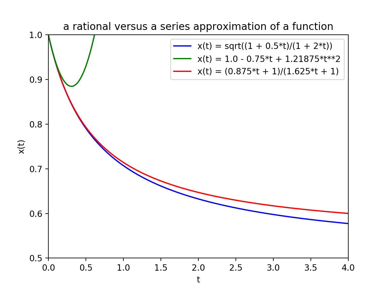
One motivation for finding a series solution is that once it is obtained, one can directly compute the associated Padé approximant, which often has much better convergence properties. Padé approximants [6] are applied in symbolic deformation algorithms [22]. In this section we reproduce [6, Figure 1.1.1] in the context of polynomial homotopy continuation. Consider the homotopy
| (1) |
The function is a solution of this homotopy.
Its second order Taylor series at is . The Padé approximant of degree one in numerator and denominator is . In Figure 1 we see that the series approximates the function only in a small interval and then diverges, whereas the Padé approximant is more accurate.
1.3 Motivating Example: Viviani’s Curve
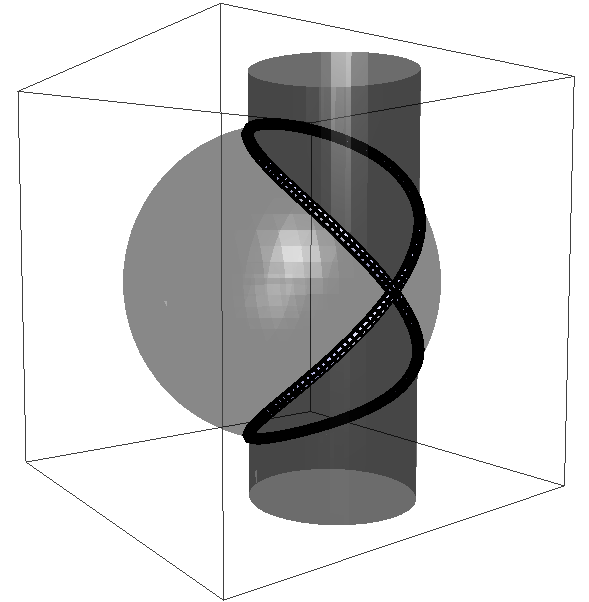
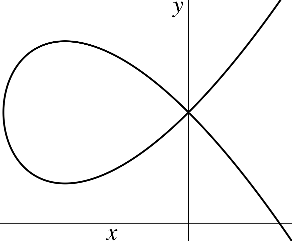
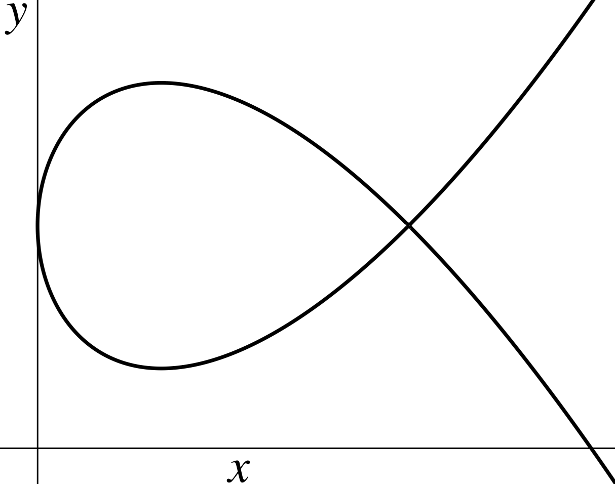
Viviani’s curve is defined as the intersection of the sphere and the cylinder such that the surfaces are tangent at a single point; see Figure 2. Our methods will allow us to find the Taylor series expansion around any point on a 1-dimensional variety, assuming we have suitable starting information. For example, the origin satisfies both equations of Viviani’s curve. This is the point where the curve intersects itself, so the curve is singular111Definition 2.1 makes this precise for general curves. there, meaning algebraically that the Jacobian drops rank, and geometrically that the tangent space does not have the expected dimension. If we apply our methods at this point, we obtain the following series solution for :
| (2) |
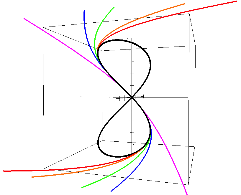
This solution is plotted in Figure 3 for a varying number of terms. To check the correctness, we can substitute (2) into the original equations, obtaining series in . The vanishing of the lower-order terms confirms that we have indeed found an approximate series solution. Such a solution, possibly transformed into an associated Padé approximant, would allow for path tracking starting at the origin.
2 The Problem and Our Solution
2.1 Problem Setup
For a polynomial system where each , the solution variety is the set of points such that . Let be a system such that the solution variety is 1-dimensional over and is not contained in the coordinate hyperplane. We seek to understand by treating the ’s as elements of , or in other words, polynomials in with coefficients in the ring of formal Laurent series . In this context we will denote the system by .
Our approach is to use Newton iteration on the system . Namely, we find some starting and repeatedly solve
| (3) |
for the update to , where is the Jacobian matrix of with respect to . This is a system of equations that is linear over , so the problem is well-posed. Computationally speaking, one approach to solving it would be to overload the operators on (truncated) power series and apply basic linear algebra techniques. A main point of our paper is that this method can be improved upon.
Of course, applying Newton’s method requires a starting guess; here we must define what it means to be singular:
Definition 2.1.
A point on a -dimensional component of a variety is regular if the Jacobian of evaluated at has rank . Points that are not regular are called singular.
In most cases the starting guess for Newton’s method can just be a point such that is in . However, if is a singular point, this is insufficient. In addition, could be a branch point (which we define later), in which case it is also not enough to use as the starting guess for Newton’s method.
We solve two problems in this paper. First, we find an effective way to perform the Newton step; the framework is established in Section 2.2, and our solution is laid out in Section 2.4. And second, we discuss the prelude to Newton’s method in Section 2.3, characterizing when techniques from tropical geometry are needed to transform the problem and obtain the starting guess.
2.2 The Newton Step
Solving the Newton step (3) amounts to solving a linear system
| (4) |
over the field . Our first step is linearization, which turns a vector of series into a series of vectors, and likewise for a matrix series. In other words, we refactor the problem and think of and as in instead of , and as in instead of .
Suppose that is the lowest order of a term in , and the lowest order of a term in . Then we can write the linearized
| (5) | ||||
| (6) | ||||
| (7) |
where and . Expanding and equating powers of , the linearized version of (4) is therefore equivalent to solving
for some . This can be written in block matrix form as
| (9) |
For the remainder of this paper, we will use and to denote vectors of series, while and will denote their linearized counterparts, that is, series which have vectors for coefficients.
Example 1.
Let
| (10) |
Starting with , the first Newton step can be written:
| (11) |
To put in linearized form, we have , ,
| (12) |
| (13) |
Since is regular, we can solve in staggered form as in (2.2), which yields the next term:
| (14) |
After another iteration, our series solution is
| (15) |
In fact this is the entire series solution for — substituting (15) into causes both polynomials to vanish completely.
Remark 1.
We constructed the example above so its solution is a series with finitely many terms, a polynomial. The solution of (4) can be interpreted as the solution obtained via Hermite interpolation. Observe that for a series
| (16) |
its Maclaurin expansion is
| (17) |
where denotes the -th derivative of evaluated at zero. Then:
| (18) |
Solving (4) up to degree implies that all derivatives up to degree of at match the solution. If the solution is a polynomial, then this polynomial will be obtained if (4) is solved up to the degree of the polynomial.
2.3 The Starting Guess, and Related Considerations
Our hope is that a solution of parameterizes the curve in some neighborhood of a point . In other words, if is the projection map of onto the -coordinate axis, then should be a branch of .
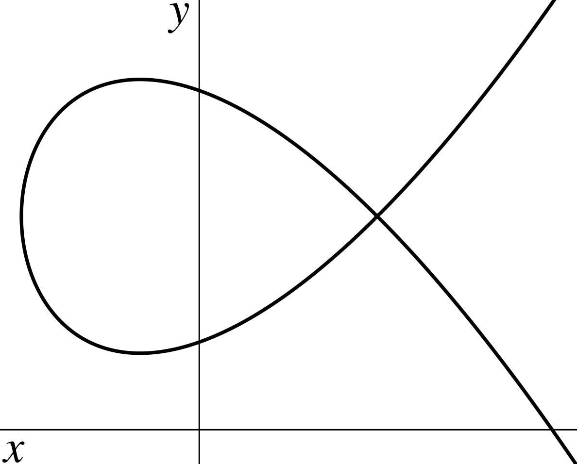
It is natural to think that there are two scenarios for the starting point , namely that it is a regular point or it is singular. And indeed, when is singular, tropical methods are required. Intuitively speaking, when at a singular point, knowing just the point itself is insufficient to determine the series; higher-derivative information is required. Observe the second frame of Figure 4.
The point being regular, however, is not enough. Consider the third frame of Figure 4. Here cannot be lifted because the origin is a branch point of the curve. In other words, the derivative at in terms of is undefined, so a Taylor series in is impossible without a transformation of the problem.
The proper way to check if Newton’s method can be applied directly to , or whether tropical methods are needed, is by checking if is a singular point of . Setting , we have . We can thus use to distinguish the first frame of Figure 4 from the latter two. This is summarized and proven in the following.
Proposition 2.2.
Let , and set . Then is a regular point of if and only if for every step of Newton’s method applied to , and has full rank.
Proof.
By definition, is a regular point of if and only if has full rank. But note that is
| (19) |
and is
| (20) |
So has full rank at if and only if has full rank at . Thus it suffices to show that after each Newton step, and remain true, so that continues to have full rank.
We clearly have at every step, since the Newton iteration cannot introduce negative exponents. At the beginning, and hold trivially. Inducting on the Newton steps, if and at some point in the algorithm, then the next , namely , is the same matrix as in the last step, hence it is again regular and is 0. Since , must be strictly greater than 0. Thus the next Newton update must have positive degree in all components, leaving unchanged.
To summarize the cases:
Lemma 2.3.
There are three possible scenarios for :
In the first case, we can simply use to start the Newton iteration. In the second, we must defer to tropical methods in order to obtain the necessary starting , which will lie in . In the final case, we also defer to tropical methods, which provide a starting that will have negative exponents. A change of coordinates brings the problem back into one of the first two cases, and we can apply our method directly. It is important to reiterate that may be a regular point of but a singular point of , as is the case in the third frame of Figure 4. The following example also demonstrates this behavior.
Example 2 (Viviani, continued).
In Section 1.3 we introduced the example of Viviani’s curve. If we translate by a substitution so that setting gives not the singular point at the origin, but instead the highest and lowest points on the curve, the system becomes
| (21) |
When we obtain the two points and , which are both regular points. For the augmented system , the Jacobian is
| (22) |
which at the point becomes
| (23) |
This matrix drops rank, hence is a singular point of and we are in the second case of Lemma 2.3. Following Lemma 2.3, we defer to tropical methods to begin, obtaining the transformation and the starting term . Now the first Newton step can be written:
| (24) |
Note that is now invertible over . Its inverse begins with negative exponents of :
| (25) |
To linearize, we first observe that and , so will have degree at least . The linearized block form of (24) is then
| (26) |
Whether we solve (24) over or solve (26) in the least squares sense, we obtain the same Newton update
| (27) |
or in non-linearized form,
| (28) |
Substituting into (21) produces , and we have obtained the desired cancellation of lower-order terms.
The matrix in (26) we call a Hermite-Laurent matrix, because its correspondence with Hermite-Laurent interpolation.
2.4 A Lower Triangular Echelon Form
When we are in the regular case of Lemma 2.3 and the condition number of is low, we can simply solve the staggered system (2.2). When this is not possible, we are forced to solve (9). Figure 5 shows the structure of the coefficient matrix (9) for the regular case, when is regular and all block matrices are dense. The essence of this section is that we can use column operations to reduce the block matrix to a lower triangular echelon form as shown at the right of Figure 5, solving (9) in the same time as (2.2).
The lower triangular echelon form of a matrix is a lower triangular matrix with zero elements above the diagonal. If the matrix is regular, then all diagonal elements are nonzero. For a singular matrix, the zero rows of its echelon form are on top (have the lowest row index) and the zero columns are at the right (have the highest column index). Every nonzero column has one pivot element, which is the nonzero element with the smallest row index in the column. All elements at the right of a pivot are zero. Columns may need to be swapped so that the row indices of the pivots of columns with increasing column indices are sorted in decreasing order.
Example 3.
(Viviani, continued). For the matrix series in (26), we have the following reduction:
| (29) |
Because of the singular matrix coefficients in the series, we find zeros on the diagonal in the echelon form.
Given a general -by- dimensional matrix , the lower triangular echelon form can be described by one -by- row permutation matrix which swaps the zero rows of and a sequence of column permutation matrices (of dimension ) and multiplier matrices (also of dimension ). The matrices define the column swaps to bring the pivots with lowest row indices to the lowest column indices. The matrices contain the multipliers to reduce what is at the right of the pivots to zero. Then the construction of the lower triangular echelon form can be summarized in the following matrix equation:
| (30) |
Similar to solving a linear system with a LU factorization, the multipliers are applied to the solution of the lower triangular system which has as its coefficient matrix.
3 Some Preliminary Cost Estimates
Working with truncated power series is somewhat similar to working with extended precision arithmetic. In this section we make some observations regarding the cost overhead.
3.1 Cost of one step
First we compare the cost of computing a single Newton step using the various methods introduced. We let denote the degree of the truncated series in , and the dimension of the matrix coefficients in as before.
The staggered system. In the case that and the leading coefficient of the matrix series is regular, the equations in (2.2) can be solved with operations. The cost is for the decomposition of the matrix , and for the back substitutions using the decomposition of and the convolutions to compute the right hand sides.
The big block matrix. Ignoring the triangular matrix structure, the cost of solving the larger linear system (9) is .
The lower triangular echelon version. If the leading coefficient in the matrix series is regular (as illustrated by Figure 5), we may copy the lower triangular echelon form of to all blocks on the diagonal and apply the permutation and column operations as defined by to all other column blocks in . The regularity of implies that we may use the lower triangular echelon form of to solve (9) with substitution. Thus with this quick optimization we obtain the same cost as solving the staggered system (2.2).
In general, and several other matrix coefficients may be rank deficient, and the diagonal of nonzero pivot elements will shift towards the bottom of . We then find as solutions vectors in the null space of the upper portion of the matrix .
3.2 Cost of computing terms
Assume that . In the regular case, assuming quadratic convergence, it will take steps to compute terms. We can reuse the factorization of at each step, so we have for the decomposition plus
| (31) |
for the back substitutions. Putting these together, we find the cost of computing terms to be .
4 Computational Experiments
Our power series methods have been implemented in PHCpack [33] and are available to the Python programmer via phcpy [34]. To set up the problems we used the computer algebra system Sage [32], and for tropical computations we used Gfan [8] and Singular [13] via the Sage interface.
4.1 The Problem of Apollonius
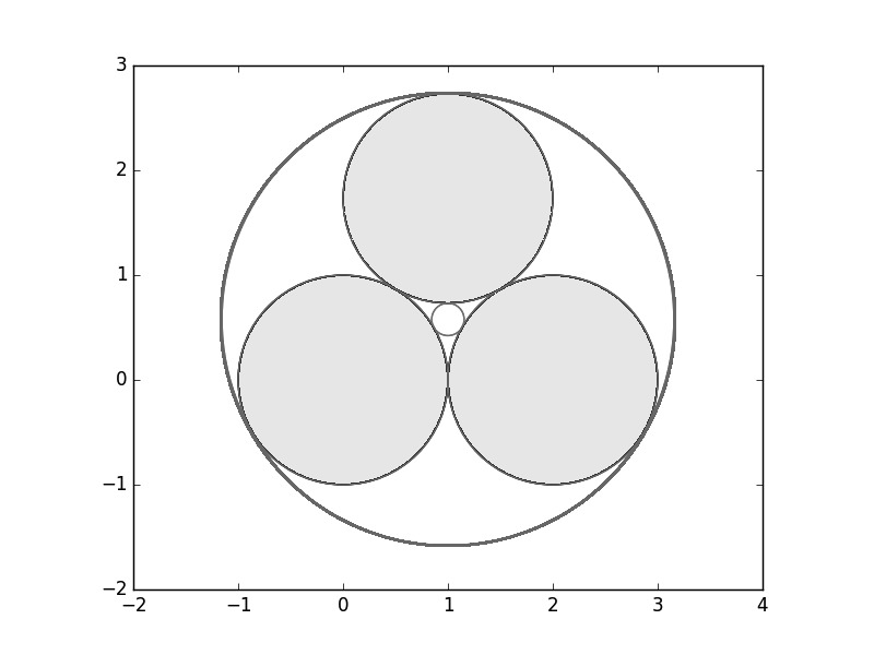
The classical problem of Apollonius consists in finding all circles that are simultaneously tangent to three given circles. A special case is when the three circles are mutually tangent and have the same radius; see Figure 6. Here the solution variety is singular – the circles themselves are double solutions. In this figure, all have radius 3, and centers , , and . We can study this configuration with power series techniques by introducing a parameter to represent a vertical shift of the upper circle. We then examine the solutions as we vary . This is represented algebraically as a solution to
| (32) |
Because we are interested in power series solutions of (32) near , we use as our free variable. To simplify away the , we substitute , , and the system becomes
| (33) |
Call this system . Now we examine the system at . The Jacobian at is
| (34) |
so — and by extension — is singular at , and we are in the second case of Lemma 2.3. Tropical methods give two possible starting solutions, which rounded for readability are and . We will continue with the second; call it . For the first step of Newton’s method, is
| (35) |
and is
| (36) |
From these we can construct the linearized system
| (37) |
Solving in the least squares sense, we obtain two more terms of the series, so in total we have
| (38) |
By comparison, the series we obtain from the other possible starting solution is
| (39) |
From these, we get a good idea of what happens near : the first solution circle grows rapidly (corresponding to the larger coefficients in (38)), while the other stays small (corresponding to the smaller coefficient in (39)). This is illustrated in Figure 7, which shows the solutions of the system at .
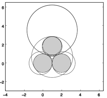
This example demonstrates the application of power series solutions in polynomial homotopies. Current numerical continuation methods cannot be applied to track the solution paths defined by the homotopy in (32), because at , the start solutions are double solutions. The power series solutions provide reliable predictions to start tracking the solution paths defined by (32).
4.2 Tangents to Four Spheres
Our next example is that of finding all lines mutually tangent to four spheres in ; see [14], [25], [30], and [31]. If a sphere has center and radius , the condition that a line in is tangent to is given by
| (40) |
where and are the moment and tangent vectors of the line, respectively. For four spheres, this gives rise to four polynomial equations; if we add the equation to require that and are perpendicular and to require that , we have a system of 6 equations in 6 unknowns which we expect to be 0-dimensional.
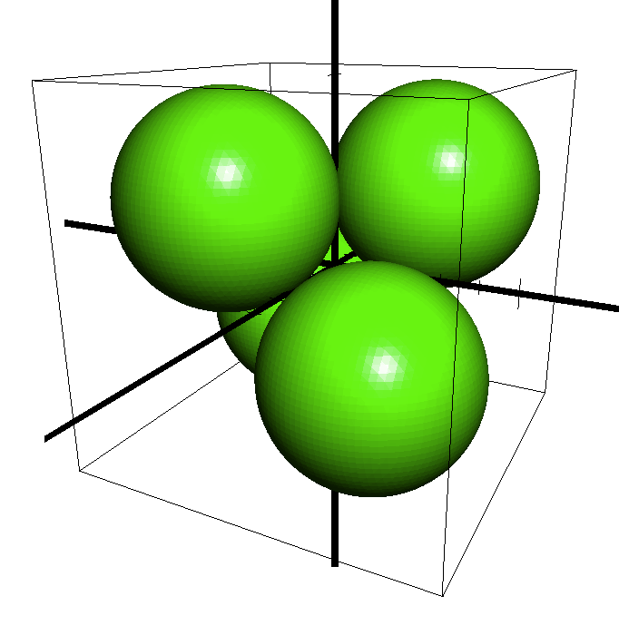
If we choose the centers to be , , , and and the radii to all be , the spheres all mutually touch and the configuration is singular; see Figure 8. In this case, the number of solutions drops to three, each of multiplicity 4.
Next we introduce an extra parameter to the equations so that the radii of the spheres are . This results in a 1-dimensional system , which we omit for succinctness. is singular at , so we are once again in the second case of Lemma 2.3. Tropical and algebraic techniques — in particular, the tropical basis [8] in Gfan [20] and the primary decomposition in Singular [13] — decompose into three systems, one of which is
| (41) |
Using our methods we can find several solutions to this, one of which is
Substituting back into yields series in , confirming the calculations. This solution could be used as the initial predictor in a homotopy beginning at the singular configuration.
In contrast to the small Apollonius circle problem, this example is computationally more challenging, as covered in [14], [25], [30], and [31]. It illustrates the combination of tropical methods in computer algebra with symbolic-numeric power series computations to define a polynomial homotopy to track solution paths starting at multiple solutions.
4.3 Series Developments for Cyclic 8-Roots
A vector of a unitary matrix is biunimodular if for : and for . The following system arises in the study [15] of biunimodular vectors:
| (42) |
Cyclic 8-roots has solution curves not reported by Backelin [5]. Note that because of the last equation, the system has no solution for , or in other words . Thus we are in the third case of Lemma 2.3.
In [1, 2], the vector gives the leading exponents of the series. The corresponding unimodular coordinate transformation is
| (43) |
Solving the transformed system with set to gives the leading coefficient of the series.
After 2 Newton steps, invoked in PHCpack with phc -u, the series for is
(-1.25000000000000E+00 + 1.25000000000000E+00*i)*z0^2
+( 5.00000000000000E-01 - 2.37676980513323E-17*i)*z0
+(-5.00000000000000E-01 - 5.00000000000000E-01*i);
After a third step, the series for is
( 7.12500000000000E+00 + 7.12500000000000E+00*i)*z0^4
+(-1.52745512076048E-16 - 4.25000000000000E+00*i)*z0^3
+(-1.25000000000000E+00 + 1.25000000000000E+00*i)*z0^2
+( 5.00000000000000E-01 - 1.45255178343636E-17*i)*z0
+(-5.00000000000000E-01 - 5.00000000000000E-01*i);
Bounds on the degree of the Puiseux series expansion to decide whether a point is isolated are derived in [18]. While the explicit bounds (which can be computed without prior knowledge of the degrees of the solution curves) are large, the test of whether a point is isolated can still be performed efficiently with our quadratically convergent Newton’s method.
In a future work, we plan to apply the power series methods to the cyclic 16-roots problem, the 16-dimensional version of this polynomial system, for which the tropical prevariety was computed recently [19].
References
- [1] D. Adrovic and J. Verschelde. Computing Puiseux series for algebraic surfaces. In J. van der Hoeven and M. van Hoeij, editors, Proceedings of the 37th International Symposium on Symbolic and Algebraic Computation (ISSAC 2012), pages 20–27. ACM, 2012.
- [2] D. Adrovic and J. Verschelde. Polyhedral methods for space curves exploiting symmetry applied to the cyclic -roots problem. In V.P. Gerdt, W. Koepf, E.W. Mayr, and E.V. Vorozhtsov, editors, Computer Algebra in Scientific Computing, 15th International Workshop, CASC 2013, Berlin, Germany, volume 8136 of Lecture Notes in Computer Science, pages 10–29, 2013.
- [3] E. L. Allgower and K. Georg. Introduction to Numerical Continuation Methods, volume 45 of Classics in Applied Mathematics. SIAM, 2003.
- [4] A. Amiraslani, R. M. Corless, L. Gonzalez-Vega, and A. Shakoori. Polynomial algebra by values. Technical report, Ontario Research Centre for Computer Algebra, 2004.
- [5] J. Backelin. Square multiples n give infinitely many cyclic n-roots. Reports, Matematiska Institutionen 8, Stockholms universitet, 1989.
- [6] G. A. Baker and P. Graves-Morris. Padé Approximants, volume 59 of Encyclopedia of Mathematics and its Applications. Cambridge University Press, 2nd edition, 1996.
- [7] D. A. Bini and B. Meini. Solving block banded block Toeplitz systems with structured blocks: Algorithms and applications. In D. A. Bini, E. Tyrtyshnikov, and P. Yalamov, editors, Structured Matrices, pages 21–41. Nova Science Publishers, Inc., Commack, NY, USA, 2001.
- [8] T. Bogart, M. Hampton, and W. Stein. groebner_fan module of Sage. The Sage Development Team, 2008.
- [9] T. Bogart, A. N. Jensen, D. Speyer, B. Sturmfels, and R. R. Thomas. Computing tropical varieties. Journal of Symbolic Computation, 42(1):54–73, 2007.
- [10] A. Bompadre, G. Matera, R. Wachenchauzer, and A. Waissbein. Polynomial equation solving by lifting procedures for ramified fibers. Theoretical Computer Science, 315(2-3):335–369, 2004.
- [11] D. Castro, L. M. Pardo, K. Hägele, and J. E. Morais. Kronecker’s and Newton’s approaches to solving: A first comparison. Journal of Complexity, 17(1):212–303, 2001.
- [12] A. Chesnokov and M. Van Barel. A direct method to solve block banded block Toeplitz systems with non-banded Toeplitz blocks. Journal of Computational and Applied Mathematics, 234(5):1485–1491, 2010.
- [13] W. Decker, G.-M. Greuel, G. Pfister, and H. Schönemann. Singular 4-1-0 — A computer algebra system for polynomial computations. http://www.singular.uni-kl.de, 2016.
- [14] C. Durand. Symbolic and Numerical Techniques for Constraint Solving. PhD thesis, Purdue University, 1998.
- [15] H. Führ and Z. Rzeszotnik. On biunimodular vectors for unitary matrices. Linear Algebra and its Applications, 484:86–129, 2015.
- [16] K. O. Geddes, S. R. Czapor, and G. Labahn. Algorithms for Computer Algebra. Kluwer Academic Publishers, 1992.
- [17] J. Heintz, T. Krick, S. Puddu, J. Sabia, and A. Waissbein. Deformation techniques for efficient polynomial equation solving. Journal of Complexity, 16(1):70–109, 2000.
- [18] M. I. Herrero, G. Jeronimo, and J. Sabia. Puiseux expansions and nonisolated points in algebraic varieties. Communications in Algebra, 44(5):2100–2109, 2016.
- [19] A. Jensen, J. Sommars, and J. Verschelde. Computing tropical prevarieties in parallel. In H.-W. Loidl, M. Monagan, and J.-C. Faugère, editors, Proceedings of the International Workshop on Parallel Symbolic Computation (PASCO 2017). ACM, 2017.
- [20] A. N. Jensen. Computing Gröbner fans and tropical varieties in Gfan. In M.E. Stillman, N. Takayama, and J. Verschelde, editors, Software for Algebraic Geometry, volume 148 of The IMA Volumes in Mathematics and its Applications, pages 33–46. Springer-Verlag, 2008.
- [21] A. N. Jensen, H. Markwig, and T. Markwig. An algorithm for lifting points in a tropical variety. Collectanea Mathematica, 59(2):129–165, 2008.
- [22] G. Jeronimo, G. Matera, P. Solernó, and A. Waissbein. Deformation techniques for sparse systems. Found. Comput. Math., 9:1–50, 2009.
- [23] E. Katz. A tropical toolkit. Expositiones Mathematicae, 27:1–36, 2009.
- [24] H. T. Kung and J. F. Traub. Optimal order of one-point and multipoint iteration. Journal of the Association of Computing Machinery, 21(4):643–651, 1974.
- [25] I. G. Macdonald, J. Pach, and T. Theobald. Common tangents to four unit balls in . Discrete and Computational Geometry, 26(1):1–17, 2001.
- [26] D. Maclagan and B. Sturmfels. Introduction to Tropical Geometry, volume 161 of Graduate Studies in Mathematics. American Mathematical Society, 2015.
- [27] A. Morgan. Solving polynomial systems using continuation for engineering and scientific problems, volume 57 of Classics in Applied Mathematics. SIAM, 2009.
- [28] S. Payne. Fibers of tropicalization. Mathematische Zeitschrift, 262:301–311, 2009.
- [29] A. Poteaux and M. Rybowicz. Good reduction of Puiseux series and applications. Journal of Symbolic Computation, 47(1):32–63, 2012.
- [30] F. Sottile. Real Solutions to Equations from Geometry, volume 57 of University Lecture Series. AMS, 2011.
- [31] F. Sottile and T. Theobald. Line problems in nonlinear computational geometry. In J.E. Goodman, J. Pach, and R. Pollack, editors, Computational Geometry - Twenty Years Later, pages 411–432. AMS, 2008.
- [32] W. A. Stein et al. Sage Mathematics Software (Version 6.9). The Sage Development Team, 2015. http://www.sagemath.org.
- [33] J. Verschelde. Algorithm 795: PHCpack: A general-purpose solver for polynomial systems by homotopy continuation. ACM Trans. Math. Softw., 25(2):251–276, 1999.
- [34] J. Verschelde. Modernizing PHCpack through phcpy. In P. de Buyl and N. Varoquaux, editors, Proceedings of the 6th European Conference on Python in Science (EuroSciPy 2013), pages 71–76, 2014.