Spin precession and spin waves in a chiral electron gas: beyond Larmor’s theorem

Abstract

Larmor’s theorem holds for magnetic systems that are invariant under spin rotation. In the presence of spin-orbit coupling this invariance is lost and Larmor’s theorem is broken: for systems of interacting electrons, this gives rise to a subtle interplay between the spin-orbit coupling acting on individual single-particle states and Coulomb many-body effects. We consider a quasi-two-dimensional, partially spin-polarized electron gas in a semiconductor quantum well in the presence of Rashba and Dresselhaus spin-orbit coupling. Using a linear-response approach based on time-dependent density-functional theory, we calculate the dispersions of spin-flip waves. We obtain analytic results for small wave vectors and up to second order in the Rashba and Dresselhaus coupling strengths $\alpha$ and $\beta$. Comparison with experimental data from inelastic light scattering allows us to extract $\alpha$ and $\beta$ as well as the spin-wave stiffness very accurately. We find significant deviations from the local density approximation for spin-dependent electron systems.

I Introduction

Larmor’s theorem LandauLifshitz ; Lipparini states that in a system of charges, all with the same charge-mass ratio $q/m$, moving in a centrally symmetric electrostatic potential and in a sufficiently weak magnetic field $\bf B$, the charges precess about the direction of the magnetic field with the frequency

$$\Omega_{L}=g\frac{qB}{2m}$$ (1)

(in SI units), where $g$ is the gyromagnetic ratio or g-factor.

In condensed-matter physics, Larmor’s theorem applies to the long-wavelength limit of spin-wave excitations in magnetic systems which are invariant under spin rotation. Yosida In particular, the electrons in a two-dimensional electron gas (2DEG) in the presence of a constant uniform magnetic field carry out a precessional motion at the single-particle Larmor frequency, despite the presence of Coulomb interactions.

If spin-rotational invariance is broken—for instance, in the presence of spin-orbit coupling (SOC)—Larmor’s theorem is no longer guaranteed to hold, and there will be corrections to $\Omega_{L}$. This was experimentally observed over three decades ago for a 2DEG in a GaAs/AlGaAs heterostructure, using electron spin resonance (ESR). Stein1983 Subsequently, several theoretical studies addressed the breaking of Larmor’s theorem in collective spin excitations in 2DEGs.Longo1993 ; Califano2006 ; Zhang2008 ; Roldan2010 ; Krishtopenko2015 ; Maiti2016 The corrections to $\Omega_{L}$ are caused by a subtle interplay between SOC and Coulomb many-body effects, which poses significant formal and computational challenges; on the other hand, this offers interesting opportunities for the experimental determination of SOC parameters and the study of many-body interactions.

In this paper, we present a joint experimental and theoretical study of the spin-wave dispersions of a partially spin-polarized 2DEG in a semiconductor quantum well. The influence of Rashba and Dresselhaus SOC on collective electronic modes in quantum wells was first theoretically predicted to cause an angular modulation of the intersubband plasmon dispersion. Ullrich2002 ; Ullrich2003 The effect was later experimentally confirmed, Baboux2012 and then extended to spin-wave dispersions.Baboux2013 ; Baboux2015 ; Baboux2016 ; Perez2016

In the absence of SOC, the real part of the spin-wave dispersion of a paramagnetic 2DEG has the following form for small wave vectors:Perez2009

$$\hbar\omega_{\rm sw}({\bf q})=Z+\frac{1}{2}S_{\rm sw}q^{2}\>,$$ (2)

where $Z$ is the bare Zeeman energy, and $S_{\rm sw}$ is the spin-wave stiffness, which depends on Coulomb many-body effects (explicit expressions for $Z$ and $S_{\rm sw}$ will be given in Section II). We recently discoveredPerez2016 that, to first order in the Rashba and Dresselhaus spin-orbit coupling strengths $\alpha$ and $\beta$, the spin-wave dispersion is unchanged apart from a chiral shift by a constant wave vector ${\bf q}_{0}$ (defined in Sec. III) which depends on $\alpha$, $\beta$ and the angle $\varphi$ between the magnetization direction and the [010] crystalline axis (see Fig. 1). In other words, to quadratic order in the wave vector, we find

$$\hbar\omega_{\rm sw}^{\rm SO}({\bf q})=Z+\frac{1}{2}S_{\rm sw}|{\bf q}+{\bf q}_{0}|^{2}+{\cal O}(\alpha^{2},\beta^{2}).$$ (3)

The spin-wave stiffness $S_{\rm sw}$ remains unchanged, to leading order in $\alpha,\beta$. The physical interpretation is that the spin wave behaves as if it were transformed into a spin-orbit twisted reference frame. This opens up new possibilities for manipulating spin waves, which may lead to new applications in spintronics.

To account for higher-order SOC effects in the spin-wave dispersion, it is sensible to rewrite Eq. (3) in a more general manner:

$$\omega_{\rm sw}^{\rm SO}({\bf q})=E_{0}(\varphi)+E_{1}(\varphi)q+E_{2}(\varphi)q^{2}\>,$$ (4)

where the coefficients $E_{0}$, $E_{1}$ and $E_{2}$ depend on the propagation direction $\varphi$ (see Fig. 1). From Eq. (3), the linear coefficient is given to leading order in SOC by $E_{1}(\varphi)=S_{\rm sw}{\bf q}\cdot{\bf q}_{0}/q$, which can be expressed asPerez2016

$$E_{1}(\varphi)=-\frac{2}{\zeta}\frac{Z}{(Z^{*}-Z)}(\alpha+\beta\sin 2\varphi)\>,$$ (5)

where $\zeta$ is the spin polarization of the 2DEG, and $Z^{*}$ is the renormalized Zeeman splitting, to be defined below in Section IIB.

We will present a linear-response approach based on time-dependent density-functional theory (TDDFT) which allows us to obtain analytical results for $E_{0}$, to second order in $\alpha,\beta$, and numerical results for $E_{1}$ and $E_{2}$ to all orders in SOC. The breaking of Larmor’s theorem is expressed in the coefficient $E_{0}$, which has $\varphi$-dependent corrections to $Z$. In Section IV we will obtain the following result to leading order in SOC:

$$E_{0}(\varphi) = Z+\frac{2\pi N_{s}}{Z^{*}f_{T}}\big{[}(\alpha^{2}+\beta^{2})(3f_{T}+2)$$ (6)

$${}+2\alpha\beta\sin(2\varphi)(f_{T}+2)\big{]},$$

where $f_{T}=(Z-Z^{*})/Z^{*}$.

Our analytical and numerical results will be compared with experimental results, obtained via inelastic light scattering. By fitting $E_{0}$, $E_{1}$ and $E_{2}$ we are able to extract values for $Z$, $\alpha$ and $\beta$ and present evidence for the $\varphi$ dependence of $E_{0}$ and $E_{2}$, which had not been considered in our earlier work.Perez2016 Comparison to theory shows significant deviations from the standard approximation in TDDFT, the adiabatic local-density approximation (ALDA). This provides new incentives to search for better exchange-correlation functionals for transverse spin excitations of electronic systems.

This paper is organized as follows. In Section II we discuss Larmor’s theorem without SOC: first, for completeness, we present a general proof for interacting many-body systems, and then we discuss Larmor’s theorem from a TDDFT perspective. This will lead to a new constraint for the exchange-correlation kernel of linear-response TDDFT. In Section III we consider the electronic states in a quantum well with SOC and an in-plane magnetic field. Section IV contains the derivation of the spin-wave dispersions from linear-response TDDFT, in the presence of SOC. In Section V we compare our theory with experimental results and discuss our findings. Section VI gives our conclusions.

II Larmor’s theorem

In this section we consider Larmor’s theorem in a 2DEG, from a general many-body perspective (the proof given in Sec. II.1 is not newLipparini but included here to keep the paper self-contained), and from the perspective of TDDFT. This will set the stage for the discussions in the following sections where the effects of SOC are included.

II.1 Long-wavelength limit of spin waves a 2DEG

Let us consider a 2DEG in the presence of a uniform magnetic field ${\bf B}=B\hat{e}_{z}$, where $\hat{e}_{z}$ is a unit vector lying in the plane of the 2DEG. The Hamiltonian is

$$\hat{H}=\sum_{i}\left[\frac{\hat{\bf p}^{2}_{i}}{2m}+\frac{Z}{2}\hat{\sigma}_{z,i}\right]+\frac{e^{2}}{2}\sum_{ij}\frac{1}{|{\bf r}_{i}-{\bf r}_{j}|}\>.$$ (7)

Here, $m$ and $e$ are the electron mass and charge, $Z=g\mu_{B}B$ is the Zeeman energy (the splitting between the spin-up and spin-down bands), and $\mu_{B}=|e|\hbar/2m$ is the Bohr magneton. For a 2DEG embedded in a semiconductor, $m$, $e$, and $g$ are replaced by the effective mass, charge and g-factor, $m^{*}$, $e^{*}$ and $g^{*}$, where $g^{*}$ could be a positive or negative number.

Since the magnetic field is applied in the plane of the 2DEG (in this section, we assume for simplicity that the 2DEG has zero thickness), its only effect is on the electron spin and there is no Landau level quantization. Later on, when we discuss quantum wells of finite width, we will exclude situations where the magnetic length $l_{B}=\sqrt{\hbar/|eB|}$ is smaller than the well width, and hence continue to disregard any orbital angular momentum contributions.

Let us define the spin-wave operator Perez2009 ; Perez2011

$$\hat{S}_{+,{\bf q}}=\frac{1}{2}\sum_{i}\hat{\sigma}_{+,i}e^{-i{\bf q}\cdot{\bf r}_{i}}\>,$$ (8)

where $\hat{\sigma}_{+}=\hat{\sigma}_{x}+i\hat{\sigma}_{y}$. This operator satisfies the Heisenberg equation of motion

$$\frac{d}{dt}\hat{S}_{+,{\bf q}}=\frac{1}{i\hbar}[\hat{S}_{+,{\bf q}},\hat{H}]=i\omega_{\rm sw}({\bf q})\hat{S}_{+,{\bf q}}\>,$$ (9)

where $\omega_{\rm sw}({\bf q})$ is the spin-wave frequency dispersion of the 2DEG. We are interested in the special case ${\bf q}=0$, and abbreviate $\omega_{\rm sw}({\bf q}=0)=\omega_{\rm sw,0}$. The operator $\hat{S}_{+,0}=\frac{1}{2}\sum_{i}\hat{\sigma}_{+,i}$ commutes with the kinetic and electron-electron interaction parts of $\hat{H}$, and we obtain

$$[\hat{S}_{+,0},\hat{H}]=\frac{Z}{4}\sum_{i}[\hat{\sigma}_{+,i},\hat{\sigma}_{z,i}]\\ =-Z\hat{S}_{+,0}\>,$$

where we used the standard commutation relations between the Pauli matrices $\hat{\sigma}_{x}$, $\hat{\sigma}_{y}$ and $\hat{\sigma}_{z}$. Together with Eq. (9), this yields

$$\frac{d}{dt}\hat{S}_{+,0}=\frac{i}{\hbar}Z\hat{S}_{+,0}\>,$$ (10)

and hence

$$\hbar\omega_{\rm sw,0}=Z\>.$$ (11)

Larmor’s theorem thus says that the long-wavelength limit of the spin-wave dispersion of a 2DEG is given by the bare Zeeman energy, regardless of the presence of Coulomb interactions. By comparison with Eq. (1) we have $\Omega_{L}=Z/\hbar$.

II.2 TDDFT perspective

TDDFT is a formally exact approach to calculate excitations in electronic systems.Gross1985 ; TDDFTbook In the most general case of a magnetic system, TDDFT can be formulated using the spin-density matrix $\underline{n}$ as basic variable, whose elements are defined as

$$n_{\sigma\sigma^{\prime}}({\bf r},t)=\langle\Psi(t)|\hat{\psi}_{\sigma^{\prime}}^{\dagger}({\bf r})\hat{\psi}_{\sigma}({\bf r})|\Psi(t)\rangle\>,$$ (12)

where $\Psi(t)$ is the time-dependent many-body wave function, and $\hat{\psi}_{\sigma}({\bf r}),\psi_{\sigma^{\prime}}^{\dagger}({\bf r})$ are fermionic field operators for spins $\sigma$ and $\sigma^{\prime}$, respectively. The spin-density matrix is diagonal for spatially uniform magnetic fields if the spin quantization axis is along the direction of the field. However, spin-flip excitations involve the transverse (off-diagonal) spin-density matrix response.

The frequency- and momentum-dependent linear-response equation for a 2DEG has the following form:

$$n_{\sigma\sigma^{\prime}}^{(1)}({\bf q},\omega)=\sum_{\tau\tau^{\prime}}\chi_{\sigma\sigma^{\prime},\tau\tau^{\prime}}^{\rm int}({\bf q},\omega)v_{\tau\tau^{\prime}}^{(1)}({\bf q},\omega)\>,$$ (13)

where $v_{\tau^{\prime}\tau^{\prime}}^{(1)}({\bf q},\omega)$ is a spin-dependent perturbation, and $\chi_{\sigma\sigma^{\prime},\tau\tau^{\prime}}^{\rm int}({\bf q},\omega)$ is the spin-density matrix response function of the interacting many-body system.

The TDDFT counterpart of Eq. (13) is

$$n_{\sigma\sigma^{\prime}}^{(1)}({\bf q},\omega)=\sum_{\tau\tau^{\prime}}\chi_{\sigma\sigma^{\prime},\tau\tau^{\prime}}({\bf q},\omega)v_{\tau\tau^{\prime}}^{(1)\rm eff}({\bf q},\omega)\>,$$ (14)

where $\chi_{\sigma\sigma^{\prime},\tau\tau^{\prime}}({\bf q},\omega)$ is the response function of the corresponding noninteracting 2DEG, and the effective perturbation is

$$\delta v_{\tau\tau^{\prime}}^{(1)\rm eff}({\bf q},\omega) = v_{\tau\tau^{\prime}}^{(1)}({\bf q},\omega)$$

$$+ \sum_{\lambda\lambda^{\prime}}\left[\frac{2\pi}{q}+f^{\rm xc}_{\tau\tau^{\prime},\lambda\lambda^{\prime}}({\bf q},\omega)\right]n_{\lambda\lambda^{\prime}}^{(1)}({\bf q},\omega).$$

Here, $f^{\rm xc}_{\tau\tau^{\prime},\lambda\lambda^{\prime}}({\bf q},\omega)$ is the exchange-correlation (xc) kernel for the spin-density matrix response of the 2DEG.

Let us now consider a noninteracting spin-polarized 2DEG with the Kohn-Sham Hamiltonian

$$\hat{h}=\sum_{i}\left[\frac{\hat{\bf p}^{2}_{i}}{2m}+\frac{Z^{*}}{2}\hat{\sigma}_{z,i}\right]\>,$$ (16)

which produces two parabolic, spin-split energy bands $\hbar^{2}k^{2}/2m+\varepsilon_{\uparrow,\downarrow}$ (spin-up and spin-down are taken with respect to the $z$ axis). In the following let us assume that $\varepsilon_{\uparrow}-\varepsilon_{\downarrow}>0$, so $\zeta<0$. The renormalized Zeeman energy is therefore given by

$$Z^{*}=\varepsilon_{\uparrow}-\varepsilon_{\downarrow}=Z+v_{\rm xc\uparrow}-v_{\rm xc\downarrow}\>.$$ (17)

From the xc energy per particle of a spin-polarized 2DEG,Attaccalite2002 $e_{\rm xc}(n,\zeta)$ (where $n$ and $\zeta$ are the density and spin polarization, respectively), the spin-dependent xc potentials are obtained as

$$v_{\rm xc\uparrow} = e_{\rm xc}+n\>\frac{\partial e_{\rm xc}}{\partial n}+(1-\zeta)\frac{\partial e_{\rm xc}}{\partial\zeta}$$ (18)

$$v_{\rm xc\downarrow} = e_{\rm xc}+n\>\frac{\partial e_{\rm xc}}{\partial n}-(1+\zeta)\frac{\partial e_{\rm xc}}{\partial\zeta}\>,$$ (19)

so the renormalized Zeeman energy isPerez2007 ; Perez2009

$$Z^{*}=Z+2\frac{\partial e_{\rm xc}}{\partial\zeta}\>.$$ (20)

Now let us calculate the collective spin-flip excitations using linear response theory. Since the ground state of the 2DEG has no transverse spin polarization, the spin-density-matrix response decouples into longitudinal and transverse channels, and we can write the associated noninteracting response functions as

$$\underline{\chi}_{L}({\bf q},\omega) = \left(\begin{array}[]{cc}\chi_{\uparrow\uparrow,\uparrow\uparrow}&\chi_{\uparrow\uparrow,\downarrow\downarrow}\\ \chi_{\downarrow\downarrow,\uparrow\uparrow}&\chi_{\downarrow\downarrow,\downarrow\downarrow}\end{array}\right)$$ (23)

$$\underline{\chi}_{T}({\bf q},\omega) = \left(\begin{array}[]{cc}\chi_{\uparrow\downarrow,\uparrow\downarrow}&\chi_{\uparrow\downarrow,\downarrow\uparrow}\\ \chi_{\downarrow\uparrow,\uparrow\downarrow}&\chi_{\downarrow\uparrow,\downarrow\uparrow}\end{array}\right),$$ (26)

and similar for the interacting case. The transverse part of the interacting response function is diagonal, and can be expressed via TDDFT as

$$\underline{\chi}_{T}^{\rm int}({\bf q},\omega)=\left(\begin{array}[]{cc}\frac{\chi_{\uparrow\downarrow,\uparrow\downarrow}}{1-\chi_{\uparrow\downarrow,\uparrow\downarrow}f^{\rm xc}_{\uparrow\downarrow,\uparrow\downarrow}}&0\\ 0&\frac{\chi_{\downarrow\uparrow,\downarrow\uparrow}}{1-\chi_{\downarrow\uparrow,\downarrow\uparrow}f^{\rm xc}_{\downarrow\uparrow,\downarrow\uparrow}}\end{array}\right).$$ (27)

We now consider the case ${\bf q}=0$, where the spin-flip Lindhard functions have the simple form

$$\chi_{\uparrow\downarrow,\uparrow\downarrow}(0,\omega) = -\frac{n\zeta}{\omega-Z^{*}}$$ (28)

$$\chi_{\downarrow\uparrow,\downarrow\uparrow}(0,\omega) = \frac{n\zeta}{\omega+Z^{*}}$$ (29)

(for a comprehensive discussion of the Lindhard function—the response function of the noninteracting electron gas—see Ref. GiulianiVignale, ). We get a collective excitation at that frequency where $\underline{\chi}_{T}^{\rm int}$ is singular. We substitute Eqs. (28) and (29) into Eq. (27) and set the determinant of the $2\times 2$ transverse response matrix $\underline{\chi}_{T}^{\rm int}$ to zero. Furthermore, because the system has no transverse spin polarization in the ground state, we have

$$f^{\rm xc}_{\uparrow\downarrow,\uparrow\downarrow}(q,\omega)=f^{\rm xc}_{\downarrow\uparrow,\downarrow\uparrow}(q,\omega)\equiv f^{\rm xc}_{T}(q,\omega)\>.$$ (30)

This yields the ${\bf q}=0$ limit of the spin-flip wave of the 2DEG as

$$\omega_{\rm sw,0}=Z^{*}-n\zeta f^{\rm xc}_{T}(0,\omega_{\rm sw,0}).$$ (31)

This expression is formally exact. Comparing with the many-body result (11), and using Eq. (20), gives

$$f^{\rm xc}_{T}(0,Z)=\frac{2}{n\zeta}\frac{\partial e_{\rm xc}}{\partial\zeta}\>.$$ (32)

Equation (32) is an exact constraint on the transverse xc kernel of the 2DEG, based on Larmor’s theorem. It is not difficult to show that it is satisfied by the adiabatic local-density approximation (ALDA), where the xc kernel is frequency- and momentum-independent.Rajagopal1978 ; Perez2009

For small but finite wave vectors, one obtains the long-wavelength spin-flip wave dispersion:Perez2009

$$\omega_{\rm sw,q}=Z-\frac{1}{|\zeta|}\frac{Z}{Z^{\ast}-Z}\frac{\hbar}{2m^{\ast}}q^{2}$$ (33)

which yields the spin-wave stiffness $S_{\rm sw}=-\frac{1}{|\zeta|}\frac{Z}{Z^{\ast}-Z}\frac{\hbar}{m^{\ast}}$, see Eq. (2).

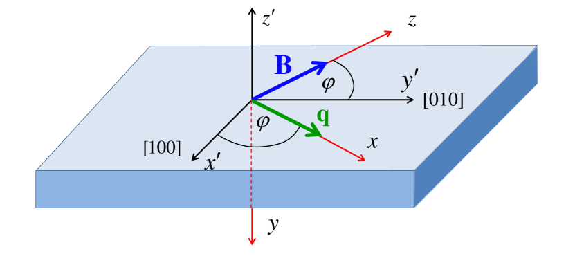
Figure 1: (Color online) Reference frames ${\cal R}^{\prime}$ (black) and $\cal R$ (red) used to describe the electronic states in a quantum well with in-plane magnetic field ${\bf B}$ and spin-wave propagation direction ${\bf q}$.

III Quantum well with in-plane magnetic field and SOC

In this Section we will consider the electronic ground state of an $n$-doped semiconductor quantum well with in-plane magnetic field and Rashba and Dresselhaus SOC, using DFT and the effective-mass approximation. The setup is illustrated in Figure 1, which defines two reference frames. The reference frame $\cal R^{\prime}$ is fixed with respect to the quantum well: the quasi-2DEG lies in the $x^{\prime}-y^{\prime}$ plane, where the $x^{\prime}$-axis points along the crystallographic [100] direction and the $y^{\prime}$-axis points along the [010] direction. The $z^{\prime}$-axis is along the direction of quantum confinement of the well.

The coordinate system $\cal R$ is oriented such that its $x-z$ plane lies in the quantum well plane, and the $z$-axis points along the in-plane magnetic field ${\bf B}$. In the inelastic light scattering experiments that we will discuss below, ${\bf B}$ is always perpendicular to the wave vector ${\bf q}$ of the spin waves. Here, ${\bf q}$ is along the $x$-axis, which is at an angle $\varphi$ with respect to the $x^{\prime}$-axis.

The single-particle states in the reference frame $\cal R^{\prime}$ can be written as

$$\Psi^{\prime}_{j{\bf k}}({\bf r}^{\prime})=e^{i{\bf k}\cdot{\bf r}^{\prime}}\psi^{\prime}_{j{\bf k}}(z^{\prime})\>.$$ (34)

Here, ${\bf k}=(k_{x^{\prime}},k_{y^{\prime}},0)$ is the in-plane wave vector and $j$ is the subband index; in the following, we are only interested in the lowest spin-split subband, so the subband index $j$ will be replaced by the index $p=\pm 1$. The two-component spinors $\psi^{\prime}_{p{\bf k}}(z^{\prime})$ are obtained from the following Kohn-Sham equation:

$$[h_{0}\hat{\sigma}_{0}+h_{x^{\prime}}\hat{\sigma}_{x^{\prime}}+h_{y^{\prime}}\hat{\sigma}_{y^{\prime}}]\psi^{\prime}_{p{\bf k}}(z^{\prime})=E_{p{\bf k}}\psi^{\prime}_{p{\bf k}}(z^{\prime})\>,$$ (35)

where $\hat{\sigma}_{0}$ is the $2\times 2$ unit matrix. The spin-independent, diagonal part of the single-particle Hamiltonian is

$$h_{0}=\frac{k^{2}}{2}-\frac{1}{2}\frac{d^{2}}{dz^{\prime 2}}+v_{\rm conf}(z^{\prime})+v_{\rm H}(z^{\prime})+v_{\rm xc}^{+}(z^{\prime})\>.$$ (36)

Here, $v_{\rm conf}(z^{\prime})$ is the quantum well confining potential (an asymmetric square well), $v_{\rm H}(z^{\prime})$ is the Hartree potential, and we define $v_{\rm xc}^{\pm}(z^{\prime})=[v_{\rm xc\uparrow}(z^{\prime})\pm v_{\rm xc\downarrow}(z^{\prime})]/2$.

The off-diagonal parts in Eq. (35) contain the Zeeman energy $Z$ plus xc and SOC contributions:

$$h_{x^{\prime}} = -\left(\frac{Z}{2}+v_{\rm xc}^{-}(z^{\prime})\right)\sin\varphi+\alpha k_{y^{\prime}}+\beta k_{x^{\prime}}$$ (37)

$$h_{y^{\prime}} = \left(\frac{Z}{2}+v_{\rm xc}^{-}(z^{\prime})\right)\cos\varphi-\alpha k_{x^{\prime}}-\beta k_{y^{\prime}}\>,$$ (38)

where $\alpha$ and $\beta$ are the standard Rashba and Dresselhaus coupling parameters.

To find the solutions of the Kohn-Sham system, it is convenient to transform into the reference system $\cal R$ of Fig. 1, whose $z$-axis is along the magnetic field direction. We introduce two in-plane vectors, ${\bf q}_{0}$ and ${\bf q}_{1}$, whose components (in the frame ${\cal R}^{\prime}$) are

$$q_{0x^{\prime}} = 2(\alpha\cos\varphi+\beta\sin\varphi)$$ (39)

$$q_{0y^{\prime}} = 2(\alpha\sin\varphi+\beta\cos\varphi)$$ (40)

and

$$q_{1x^{\prime}} = 2(-\alpha\sin\varphi+\beta\cos\varphi)$$ (41)

$$q_{1y^{\prime}} = 2(\alpha\cos\varphi-\beta\sin\varphi)\>.$$ (42)

With this, Eq. (35) transforms into

$$\left[h_{0}\hat{\sigma}_{0}+\left(\frac{Z-{\bf k}\cdot{\bf q}_{0}}{2}+v_{\rm xc}^{-}\right)\hat{\sigma}_{z}+\frac{{\bf k}\cdot{\bf q}_{1}}{2}\hat{\sigma}_{x}\right]\psi_{p{\bf k}}=E_{p{\bf k}}\psi_{p{\bf k}}$$ (43)

(the scalar products ${\bf k}\cdot{\bf q}_{0}$ and ${\bf k}\cdot{\bf q}_{1}$ are invariant under this coordinate transformation). The solutions of Eq. (43) can be written as follows:

$$E_{p{\bf k}}=\frac{k^{2}}{2}+\frac{\varepsilon_{\uparrow}+\varepsilon_{\downarrow}}{2}+\frac{p}{2}\sqrt{\left(Z^{*}-{\bf k}\cdot{\bf q}_{0}\right)^{2}+({\bf k}\cdot{\bf q}_{1})^{2}}\>,$$ (44)

where $Z^{*}=\varepsilon_{\uparrow}-\varepsilon_{\downarrow}$ and $p=\pm 1$. The associated eigenfunctions are

$$\psi_{+,{\bf k}}(y) = \frac{1}{\sqrt{1+b^{2}}}\left(\begin{array}[]{c}1\\ b\end{array}\right)\phi(y)$$ (47)

$$\psi_{-,{\bf k}}(y) = \frac{1}{\sqrt{1+b^{2}}}\left(\begin{array}[]{c}-b\\ 1\end{array}\right)\phi(y)$$ (50)

and

$$b=\frac{1}{{\bf k}\cdot{\bf q}_{1}}\left[\sqrt{\left(Z^{*}-{\bf k}\cdot{\bf q}_{0}\right)^{2}+({\bf k}\cdot{\bf q}_{1})^{2}}-Z^{*}+{\bf k}\cdot{\bf q}_{0}\right].$$ (51)

The solutions (44)–(51) have been expressed in terms of the solutions in the absence of SOC, $\varepsilon_{\uparrow,\downarrow}$ and $\phi(y)$, which follow from

$$\left[h_{0}\pm\left(\frac{Z}{2}+v_{\rm xc}^{-}\right)\right]\phi_{\uparrow,\downarrow}=\varepsilon_{\uparrow,\downarrow}\phi_{\uparrow\downarrow}\>.$$ (52)

The spin-up and spin-down envelope functions $\phi_{\uparrow}$ and $\phi_{\downarrow}$ are practically identical for the systems considered here, which allowed us to use $\phi_{\uparrow}\approx\phi_{\downarrow}\equiv\phi$ to express the solutions (47) and (50) in a relatively compact form.

Finally, let us expand the solutions (44)–(51) in powers of the SOC coefficients $\alpha$ and $\beta$. We obtain to second order in SOC

$$E_{p{\bf k}}=\frac{k^{2}}{2}+\frac{\varepsilon_{\uparrow}+\varepsilon_{\downarrow}}{2}+\frac{p}{2}\!\left(Z^{*}-{\bf k}\cdot{\bf q}_{0}+\frac{({\bf k}\cdot{\bf q}_{1})^{2}}{2Z^{*}}\right)$$ (53)

and

$$\psi_{+}(y) = \left(\begin{array}[]{c}\displaystyle 1-\frac{({\bf k}\cdot{\bf q}_{1})^{2}}{8Z^{*2}}\\[5.69054pt] \displaystyle\frac{{\bf k}\cdot{\bf q}_{1}}{2Z^{*}}+\frac{({\bf k}\cdot{\bf q}_{0})({\bf k}\cdot{\bf q}_{1})}{2Z^{*2}}\end{array}\right)\!\phi(y)$$ (56)

$$\psi_{-}(y) = \left(\begin{array}[]{c}\displaystyle-\frac{{\bf k}\cdot{\bf q}_{1}}{2Z^{*}}-\frac{({\bf k}\cdot{\bf q}_{0})({\bf k}\cdot{\bf q}_{1})}{2Z^{*2}}\\[5.69054pt] \displaystyle 1-\frac{({\bf k}\cdot{\bf q}_{1})^{2}}{8Z^{*2}}\end{array}\right)\!\phi(y).$$ (59)

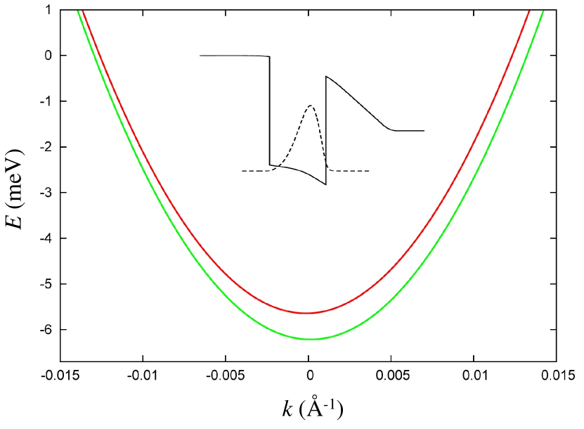
Figure 2: (Color online) Spin-split lowest subband, Eq. (44), of an asymmetrically doped 20 nm CdTe quantum well with $B=4.18$ T, with $\alpha=2.2$ meVÅ and $\beta=3.9$ meVÅ, taken at an angle $\varphi=45^{\rm o}$ (i.e. along [110]). The inset shows the quantum well profile and the electronic density distribution.

We illustrate the energy dispersion (44) of the lowest spin-split subband in Fig. 2. Here, we consider an asymmetrically doped CdMn quantum well of width 20 nm and electron density $2.6\times 10^{11}$ $\rm cm^{-1}$. An applied magnetic field of $B=4.18$ T leads to the bare and renormalized Zeeman energies $Z=0.40$ meV and $Z^{*}=0.573$ meV, respectively, using the LDA. Here, we use the effective-mass parameters $m^{*}=0.105m$, $e^{*}=1/\sqrt{10}$, and $g^{*}=-1.64$ for CdTe.

We choose the Rashba and Dresselhaus parameters $\alpha=2.2$ meVÅ and $\beta=3.9$ meVÅ (see below), which causes the two subband to be slightly displaced horizontally with respect to one another (in Fig. 2, we plot $k$ along the [110] direction, i.e., for $\varphi=45^{\rm o}$).

IV Spin-flip waves dispersion

IV.1 Linear-response formalism

In the following, we are interested in the collective spin-flip modes in a quantum well with in-plane magnetic field and SOC. Based on the translational symmetry in the $x-z$ plane, one can Fourier transform with respect to the in-plane position vector ${\bf r}=(x,z)$; this introduces the in-plane wave vector ${\bf q}$. The TDDFT linear-response equation (14) then becomes

$$n^{(1)}_{\sigma\sigma^{\prime}}({\bf q},y,\omega)=\sum_{\tau\tau^{\prime}}\int dy^{\prime}\chi_{\sigma\sigma^{\prime},\tau\tau^{\prime}}({\bf q},y,y^{\prime},\omega)v^{(1)\rm eff}_{\tau\tau^{\prime}}({\bf q},y^{\prime},\omega),$$ (60)

where the noninteracting response function is given by

$$\chi_{\sigma\sigma^{\prime},\tau\tau^{\prime}}({\bf q},y,y^{\prime},\omega)=$$

$$-\sum_{pp^{\prime}}^{\pm 1}\int\!\frac{d^{2}k}{(2\pi)^{2}}\>\frac{\theta(E_{F}-E_{p{\bf k}})}{\omega-E_{p{\bf k}}+E_{p^{\prime}{\bf k}-{\bf q}}+i\eta}$$

$${}\times\psi_{p\sigma}({\bf k},y)\psi^{*}_{p^{\prime}\sigma^{\prime}}({\bf k}-{\bf q},y)\psi^{*}_{p\tau}({\bf k},y^{\prime})\psi_{p^{\prime}\tau^{\prime}}({\bf k}-{\bf q},y^{\prime})$$

$${}+\sum_{pp^{\prime}}^{\pm 1}\int\!\frac{d^{2}k}{(2\pi)^{2}}\>\frac{\theta(E_{F}-E_{p{\bf k}})}{\omega+E_{p{\bf k}}-E_{p^{\prime}{\bf k}+{\bf q}}+i\eta}$$

$${}\times\psi_{p^{\prime}\sigma}({\bf k}+{\bf q},y)\psi^{*}_{p\sigma^{\prime}}({\bf k},y)\psi^{*}_{p^{\prime}\tau}({\bf k}+{\bf q},y^{\prime})\psi_{p\tau^{\prime}}({\bf k},y^{\prime}).$$

The energy eigenvalues $E_{p{\bf k}}$ and the single-particle states $\psi_{p\sigma}({\bf k},y)$ are defined in Eqs. (53)–(59). $\theta$ is the step function, and the Fermi energy is given by $E_{F}=\pi N_{s}-(\alpha^{2}+\beta^{2})$, where $N_{s}$ is the electronic sheet density (the number of electrons per unit area). We assume here that both spin-split subbands are occupied, which is different from the situation considered in Refs. Ashrafi2012, ; Maiti2015a, ; Maiti2015b, .

In the response function (IV.1) we only consider spin-flip excitations within the lowest spin-split subband of the quantum well; contributions from higher subbands are ignored, because they will be irrelevant as long as the Zeeman splitting is small compared to the separation between the lowest and higher subbands, which is safely the case here.

An interesting property of the response equation (60) is that it is invariant under the simultaneous sign changes $\alpha\to-\alpha$, $\beta\to-\beta$, and ${\bf q}\to-{\bf q}$, as can easily be seen from the form of the response function (IV.1). From this we conclude that an expansion of the coefficients $E_{0}$ and $E_{2}$ in Eq. (4) only has even orders of $\alpha,\beta$, while only odd orders of $\alpha,\beta$ contribute to $E_{1}$.

The $4\times 4$ matrix response equation (60) can be solved numerically, within the ALDA, to yield the spin-wave dispersions. Ullrich2002 ; Ullrich2003 However, much physical insight can be gained by an analytic treatment, which can be done for small wave vectors ${\bf q}$: the spin-wave dispersion then takes on the form of Eq. (4), and our goal is to determine the coefficients $E_{0}$ and $E_{2}$ and compare them to experiment. We have done this analytically for $E_{0}$ and numerically for $E_{2}$, as discussed below.

Instead of the spin-density-matrix response (60), it is convenient to work with the density-magnetization response: we replace the spin-density matrix $n_{\sigma\sigma^{\prime}}$, defined in Eq. (12), with the total density $n\equiv m_{0}$ and the three components of the magnetization $m_{x,y,z}$ as basic variables. In the following, we replace the labels $(x,y,z)$ with $(1,2,3)$ to streamline the notation.

The connection between the two sets of variables is made via the Pauli matrices:

$$m_{i}({\bf r})=\mbox{tr}\{\hat{\sigma}_{i}\underline{n}({\bf r})\}\>,\qquad i=0,\ldots,3.$$ (62)

We can also express this through a $4\times 4$ transformation matrix $\underline{\underline{T}}$, connecting the elements $m_{i}$ and $n_{\sigma\sigma^{\prime}}$ arranged as column vectors: $\vec{m}=\underline{\underline{T}}\vec{n}$. In detail,

$$\left(\begin{array}[]{c}m_{0}\\ m_{1}\\ m_{2}\\ m_{3}\end{array}\right)=\left(\begin{array}[]{cccc}1&0&0&1\\ 0&1&1&0\\ 0&i&-i&0\\ 1&0&0&-1\end{array}\right)\left(\begin{array}[]{c}n_{\uparrow\uparrow}\\ n_{\uparrow\downarrow}\\ n_{\downarrow\uparrow}\\ n_{\downarrow\downarrow}\end{array}\right).$$ (63)

In a similar way, one can transform the spin-density-matrix response equation (60) into the response equation for the density-magnetization:

$$m^{(1)}_{i}({\bf q},y,\omega)=\sum_{k=0}^{3}\int dy^{\prime}\Pi_{ik}({\bf q},y,y^{\prime},\omega)V^{(1)}_{k}({\bf q},y^{\prime},\omega)\>,$$ (64)

where $\underline{\underline{\Pi}}=2\underline{\underline{T}}\,\underline{\underline{\chi}}\,\underline{\underline{T}}^{-1}$ is the noninteracting density-magnetization response function, and $\vec{V}^{(1)}=\frac{1}{2}\underline{\underline{T}}\vec{v}^{(1)\rm eff}$ is the effective perturbing potential.

We are only interested in the spin-flip excitations, which are eigenmodes of the system: hence, no external perturbation is necessary. Furthermore, the Hartree contributions drop out in the spin channel, so the effective potential only consists of the xc part:

$$V^{(1)}_{k}({\bf q},y,\omega)=\sum^{3}_{l=0}\int dy^{\prime}h^{\rm xc}_{kl}({\bf q},y,y^{\prime},\omega)m^{(1)}_{l}({\bf q},y^{\prime},\omega)\>.$$ (65)

In the ALDA, the xc kernels $h^{\rm xc}_{kl}$ do not depend on frequency and wave vector.Ullrich2002 Once we have the density-magnetization response, we can multiply it with the xc matrix. The xc matrix has a simple form, because in this reference frame the spin polarization direction is along $z$:

$$\underline{\underline{H}}^{\rm xc}=\left(\begin{array}[]{cccc}h^{\rm xc}_{00}&0&0&h^{\rm xc}_{03}\\ 0&h^{\rm xc}_{11}&0&0\\ 0&0&h^{\rm xc}_{22}&0\\ h^{\rm xc}_{30}&0&0&h^{\rm xc}_{33}\end{array}\right)$$ (66)

where

$$h^{\rm xc}_{00} = 2\frac{\partial e_{\rm xc}}{\partial n}+n\frac{\partial^{2}e_{\rm xc}}{\partial n^{2}}-2\zeta\frac{\partial^{2}e_{\rm xc}}{\partial n\partial\zeta}+\frac{\zeta^{2}}{n}\frac{\partial^{2}e_{\rm xc}}{\partial n^{2}}$$ (67)

$$h^{\rm xc}_{03} = h^{\rm xc}_{30}=\frac{\partial^{2}e_{\rm xc}}{\partial n\partial\zeta}-\frac{\zeta}{n}\frac{\partial^{2}e_{\rm xc}}{\partial\zeta^{2}}$$ (68)

$$h^{\rm xc}_{11} = h^{\rm xc}_{22}=\frac{1}{n\zeta}\frac{\partial e_{\rm xc}}{\partial\zeta}$$ (69)

$$h^{\rm xc}_{33} = \frac{1}{n}\frac{\partial^{2}e_{\rm xc}}{\partial\zeta^{2}}\>.$$ (70)

All quantities are evaluated at the local density $n(y)$ and spin polarization $\zeta(y)$ and multiplied with $\delta(y-y^{\prime})$. Here, $e_{\rm xc}$ is the xc energy per particle of the 3D electron gas.Perdew1992

To find the collective modes, we can recast the response equation (64) in such a way that the $y$-dependence goes away; the xc kernels $h^{\rm xc}_{kl}$ are then replaced by their averages over $\phi^{4}(y)$. We need to determine those frequencies where the matrix

$$\underline{\underline{M}}({\bf q},\omega)=\underline{\underline{H}}^{\rm xc}({\bf q},\omega)\underline{\underline{\Pi}}({\bf q},\omega)$$ (71)

has the eigenvalue 1. In other words, we solve the $4\times 4$ eigenvalue problem

$$\underline{\underline{M}}({\bf q},\omega)\vec{x}=\lambda({\bf q},\omega)\vec{x}$$ (72)

and find the mode frequencies by solving $\lambda({\bf q},\omega)=1$ for $\omega$, where ${\bf q}$ is fixed. In general there will be 4 solutions. This is in principle exact, provided we know the exact Hxc matrix, which, in general, depends on $({\bf q},\omega)$. In ALDA, it is a constant (for given density and spin polarization).

IV.2 Beyond Larmor’s theorem: leading SOC corrections

In the presence of SOC, the spin-wave dispersions are modified in an interesting and subtle manner. For small values of ${\bf q}$, the spin-wave dispersion has the quadratic form given in Eq. (4). Our goal is now to obtain the coefficient $E_{0}$ to leading order in the Rashba and Dresselhaus coupling strengths $\alpha$ and $\beta$. To do this, we carry out a perturbative expansion of the eigenvalue problem (72) in orders of SOC. At $q=0$, the matrix can be written as

$$\underline{\underline{M}}(0,\omega)=\underline{\underline{M}}^{(0)}+\underline{\underline{M}}^{(2)}+\ldots\$$ (73)

where superscripts indicate the order of SOC (the linear order vanishes at $q=0$).

We first solve the zero-order eigenvalue problem $\underline{\underline{M}}^{(0)}\vec{x}^{(0)}=\lambda^{(0)}\vec{x}^{(0)}$. The zero-order spin-flip response function is

$$\underline{\underline{\Pi}}^{(0)}(0,y,y^{\prime},\omega)=\frac{Z^{*}\phi^{2}(y)\phi^{2}(y^{\prime})}{\pi(\omega^{2}-{Z^{*}}^{2})}\left(\begin{array}[]{cccc}0&0&0&0\\ 0&Z^{*}&-i\omega&0\\ 0&i\omega&Z^{*}&0\\ 0&0&0&0\end{array}\right)\>.$$ (74)

Defining

$$f_{T}=\int dy\frac{\phi^{4}(y)}{\pi n(y)\zeta(y)}\left.\frac{\partial e_{\rm xc}}{\partial\zeta}\right|_{n(y),\zeta(y)}\>,$$ (75)

where $f_{T}<0$, we obtain

$$\underline{\underline{M}}^{(0)}=\frac{Z^{*}f_{T}}{\omega^{2}-{Z^{*}}^{2}}\left(\begin{array}[]{cccc}0&0&0&0\\ 0&Z^{*}&-i\omega&0\\ 0&i\omega&Z^{*}&0\\ 0&0&0&0\end{array}\right).$$ (76)

This matrix has eigenvalue 1 for

$$\omega=Z^{*}+Z^{*}f_{T}=Z$$ (77)

(we discard the negative-frequency solution) in accordance with Larmor’s theorem. The associated eigenvector is $\vec{x}^{(0)}=2^{-1/2}(0,-i,1,0)$.

To obtain the change of the collective spin precession caused by the presence of SOC, we need to determine $\lambda^{(2)}$. Using perturbation theory we obtain the second-order correction of the eigenvalue as

$$\lambda^{(2)}=[\vec{x}^{(0)}]^{\dagger}\underline{\underline{M}}^{(2)}\vec{x}^{(0)}\>,$$ (78)

To construct $\underline{\underline{M}}^{(2)}$ we need $\underline{\underline{\Pi}}^{(2)}(0,\omega)$, the spin-flip response matrix expanded to second order in $\alpha$ and $\beta$, which requires a rather lengthy calculation (see supplemental materialsupplemental ). We end up with

$$\lambda^{(2)}=\frac{2\pi N_{s}}{{Z^{*}}^{2}f_{T}^{2}}\big{[}(\alpha^{2}+\beta^{2})(3f_{T}+2)+2\alpha\beta\sin(2\varphi)(f_{T}+2)\big{]}$$ (79)

The condition $1=\lambda^{(0)}+\lambda^{(2)}$ gives the final result for $E_{0}$, see Eq. (6).

Let us now turn to the other two coefficients in Eq. (4). The leading contribution to the linear coefficient $E_{1}$ is in first order in $\alpha$ and $\beta$, see Eq. (5), and was already obtained in Ref. Perez2016, . The quadratic coefficient $E_{2}$ describes the renormalization of the spin-wave stiffness $S_{\rm sw}$ due to SOC. We did not attempt to derive an analytical expression for $E_{2}$, as it was done without SOC in Eq. (33), although this could in principle (and with much effort) be done along the same lines as for $E_{0}$. Instead, we extract $E_{2}$ from a fully numerical solution of the linear-response equation for the spin waves, which includes all orders of $\alpha$ and $\beta$.

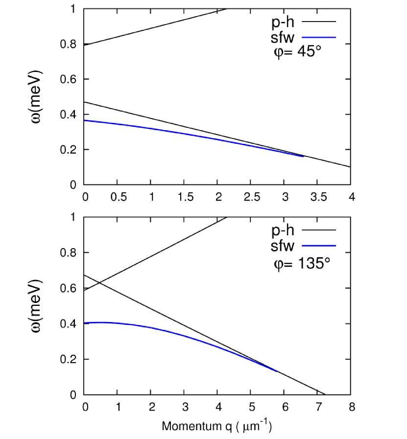
Figure 3: (Color online) Spin-flip excitation spectra with SOC for $\varphi=45^{\rm o}$ and $\varphi=135^{\rm o}$, calculated using the ALDA for the same quantum well as in Fig. 2. Solid black lines: boundaries of the single-particle spin-flip continuum. Blue dashed lines: spin-wave dispersions.

V Results and discussion

According to the theory presented above, the spin-flip excitations in a 2DEG in the presence of SOC depend on the direction of the applied magnetic field (direction $z$ in Fig. 1). Figure 3 depicts the spin-excitation spectra for $\varphi=45^{\rm o}$ and $\varphi=135^{\rm o}$, calculated using ALDA, for the same quantum well as in Fig. 2. Clearly, the spin-wave dispersions and single-particle spin-flip continua differ drastically, depending on the direction of the in-plane momentum. In the following, we will compare our theory with experiment.

V.1 Electronic Raman scattering

We use electronic Raman scattering, whereby a well-controlled in-plane momentum ${\bf q}$ is transferred to the spin excitations of the 2DEG. Under the quasi-scattering geometry shown in Fig. 4a, the transferred momentum is given by ${\bf q}=\boldsymbol{\kappa}_{i,\parallel}-{\boldsymbol{\kappa}}_{s,\parallel}\simeq\frac{4\pi}{\lambda}\sin\theta\,\boldsymbol{e}_{x}$, where $\boldsymbol{\kappa}_{i}$ and $\boldsymbol{\kappa}_{s}$ are the wave vectors of the linearly cross-polarized incoming and scattered photons, and $\lambda$ is the incoming wavelength. Our setup allows us to vary ${\bf q}$ both in magnitude and in-plane orientation, while the magnetic field $\mathbf{B}_{\mathrm{ext}}$ is applied in the plane of the well and always perpendicular to $\mathbf{q}$.

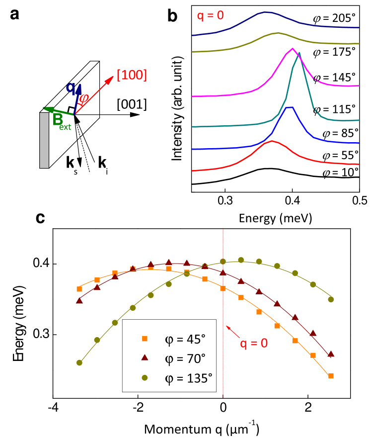
Figure 4: (Color online) (a) Electronic Raman scattering geometry: $\boldsymbol{k}_{i}$ and $\boldsymbol{k}_{s}$ are the incoming and scattered light wave vectors, respectively; $\mathbf{q}$ is the transferred momentum, of in-plane orientation measured by the angle $\varphi$ from $[100]$. An external magnetic field $\mathbf{B}_{\mathrm{ext}}$ is applied perpendicularly to $\mathbf{q}$. (b) Raman spectra of the spin wave, obtained at $B_{\mathrm{ext}}=2$ T and $q=0$, for a series of in-plane angles $\varphi$. (c) Momentum dispersion of the spin wave for different in-plane angles.

Our sample is an asymmetrically modulation-doped, $20$ nm-thick Cd_1-xMn_xTe ($x\simeq 0.13\%$) quantum well, grown along the $\left[001\right]$ direction by molecular beam epitaxy, and immersed in a superfluid helium bath at temperature 2 K. The density of the electron gas is $N_{s}=2.6\times 10^{11}$ cm^-2 and the mobility is $1.7\times 10^{5}$ cm²V^-1s^-1. The small concentration of Mn introduces localized magnetic moments into the quantum well, which are polarized by the external $B$-field, and act to amplify it.Perez2007 ; footnote

Figure 4b shows a series of spin-wave Raman lines obtained at fixed $B_{\mathrm{ext}}=2$ T and $q=0$, and for various in-plane angles $\varphi$. We observe a clear modulation of the spin-wave energy with $\varphi$, evidencing the above predicted breakdown of Larmor’s theorem.

To better understand the phenomenon, we measure the full spin-wave dispersion by varying the transferred momentum $q$. Fig. 4c shows the dispersions for three different values of $\varphi$: they exhibit a quadratic dependence with $q$, with a maximum shifted from the zone center. This shift from the zone center is well understood in the frame of the spin-orbit twist model: Perez2016 SOC produces a rigid shift of the spin-wave dispersion by a momentum $-{\bf q_{0}}$, see Eq. (39), which depends on $\varphi$. This produces the linear term in $q$ in the energy dispersion of Eq. (4).

We have systematically measured the spin-wave dispersions for angles $\varphi$ between zero and $360^{\rm o}$; for each angle, the data are fit to a parabola (as in Fig. 4c), which allows us to extract the coefficients $E_{0,1,2}(\varphi)$. The experimental results are shown in both Figs. 5 and 6 (dots), clearly exhibiting the predicted sinusoidal modulations.

The modulation of $E_{0}$, with a relative amplitude of about 6%, demonstrates the breakdown of Larmor’s theorem. This effect is of second order in the SOC. By contrast, the modulation of $E_{1}$ is a first-order SOC effect. Another second-order SOC effect is the modulation of the curvature of the spin-wave dispersion, i.e. the spin-wave stiffness $S_{\rm sw}$. The bottom panels of Figs. 5 and 6 show the curvature $E_{2}=S_{\rm sw}/2$ as a function the in-plane angle $\varphi$. Again, a sinusoidal variation is observed, with a relative amplitude of about $10\%$; the phase of the modulation is opposite to that of $E_{0}$ and $E_{1}$.

V.2 Comparison with theory

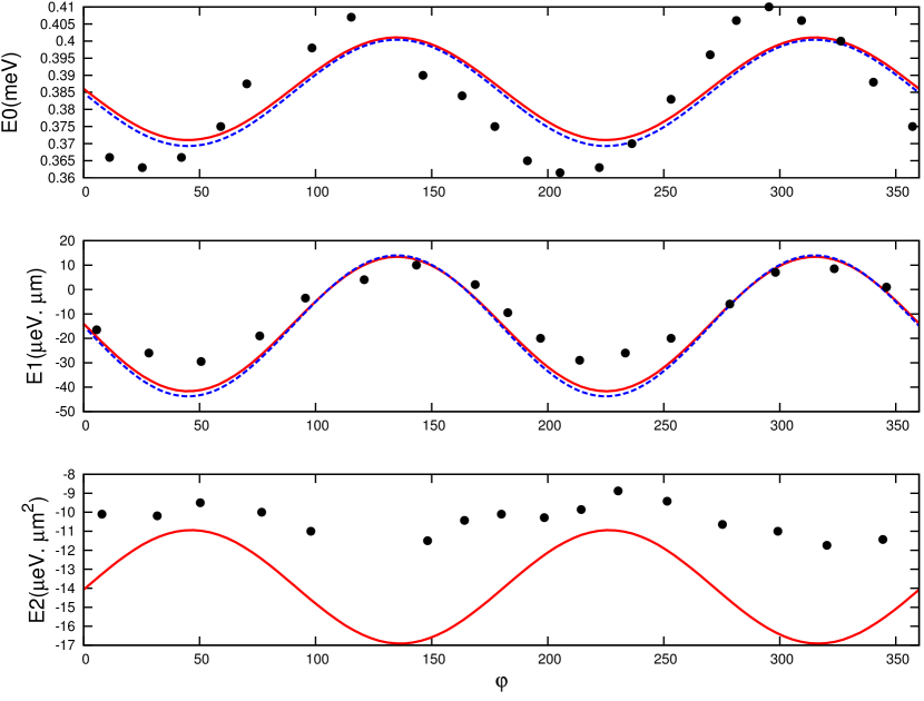
Figure 5: (Color online) Coefficients $E_{0}$, $E_{1}$, and $E_{2}$ of the spin-wave dispersion, Eq. (4), as a function of angle $\varphi$. Dots: experimental data. Lines: theoretical results using $Z^{*}=0.573$ meV obtained with ALDA, and $\alpha=1.6$ meVÅ and $\beta=3.1$ meVÅ obtained by fitting $E_{0}$ and $E_{1}$. The red lines follow from the fully numerical solution of Eq. (72), the dashed blue lines follow from the analytical formulas (6) and (5).

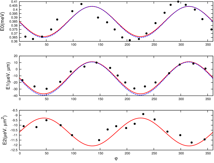
Figure 6: (Color online) Same as Fig. 5, but using $Z^{*}=0.63$ meV, $\alpha=2.2$ meVÅ, and $\beta=3.9$ meVÅ obtained from a best fit to the experimental data.

In Figures 5 and 6, the experimental data for $E_{0}(\varphi)$, $E_{1}(\varphi)$, and $E_{2}(\varphi)$ is compared with theory (lines). In our calculations, we consider, as before, a CdTe quantum well of width 20 nm and density $N_{s}=2.6\times 10^{11}$ $\rm cm^{-2}$. The value of bare Zeeman splitting $Z$ is extracted from the data as follows. According to Eq. (6), $E_{0}$ can be written in the form $E_{0}(\varphi)=Z-a-b\sin(2\varphi)$. For the range of input parameters $\alpha$, $\beta$, $Z$ and $Z^{*}$ under consideration (see below), the ratio $b/a\approx 1.5$ is almost constant. We temporary fix this ratio, and a fit with the data from the top panel of Fig. 5 then yields $Z=0.40$ meV and $b=0.024$ meV to within about 3 $\mu$eV. We can then calculate $Z^{*}$ using the ALDA xc kernel [see Eq. (77)], where $Z^{*}_{\rm ALDA}=Z/(1+f_{T})=0.573$ meV. Now fixing $Z$, $Z^{*}$ and letting $b/a=1.5$, we fit $\alpha$ and $\beta$ from $E_{0}(\varphi)$ and $E_{1}(\varphi)$. An optimal agreement with the experimental results for $E_{0}$ and $E_{1}$ is achieved with $\alpha=1.6$ meVÅ and $\beta=3.1$ meVÅ.

Having determined the set of parameters $Z$, $Z^{*}$, $\alpha$ and $\beta$, we run the fully numerical solution of the linear-response equation (72) for the spin-flip waves, and fit the small-$q$ dispersion to a parabola for a given angle $\varphi$ to extract $E_{0}$, $E_{1}$, and $E_{2}$. As shown in Fig. 5, both the analytical formulas of Eqs. (5) and (6) and the numerical solutions (the dashed blue and solid red lines, respectively) are in very good agreement with the experimental data for $E_{0}$ and $E_{1}$, apart from a shift in the phase of the experimental modulation of $E_{0}$, which is not accounted for by the theory. It is likely due to an in-plane anisotropy of the g-factor, Eldridge2013 neglected in the above analysis.

An additional observation from Fig. 5 is that the analytical formulas and the numerical results for $E_{0}$ and $E_{1}$ are extremely close to each other. This is not surprising, since the next higher-order corrections to $E_{0}$ and $E_{1}$ are of fourth and third order in $\alpha,\beta$, respectively (as we showed in Section IV.A), and hence negligible.

On the other hand, the bottom panel of Fig. 5 shows that the calculation dramatically fails to reproduce $E_{2}$. Therefore, we repeated the calculations, but now using a renormalized Zeeman energy $Z^{*}$ that does not follow from the ALDA, but from a numerical fit. We fit the numerical solutions with $Z^{*}$, $\alpha$ and $\beta$ and then find that using $\alpha=2.2$ meVÅ, $\beta=3.9$ meVÅ and $Z^{*}_{\rm fit}=0.63$ meV we obtain an excellent agreement with the experimental results for all three modulation parameters, $E_{0}$, $E_{1}$, and $E_{2}$, as shown in Fig. 6.

The comparison between theory and experiment of the spin-wave modulation parameters thus demonstrates that the ALDA underestimates $Z^{*}$ by about 10%, which seems to be a relatively minor deviation. However, $E_{0}$, $E_{1}$, and $E_{2}$ depend very sensitively on $Z^{*}$, which suggests a need for a more accurate description of dynamical xc effects beyond the ALDA.

V.3 Density dependence of $E_{0}$

To further test our theoretical prediction for the breakdown of Larmor’s theorem [Eq. (6)], we will now explore the density dependence of the parameter $E_{0}$. In order to vary the electronic density in our sample, we shine an additional continuous-wave green laser beam ($514.5$ nm) on the quantum well. This illumination is above the band gap and generates electron-hole pairs in the barrier layer: the electrons neutralize some donor elements of the doping plane, while the holes migrate to the quantum well where they capture free electrons. This leads to a depopulation of the electron gas, which can be precisely controlled by the power of the above-gap illumination.Baboux2015 Using this technique, the density in our sample can be reproducibly reduced by up to a factor $2$. We measured $E_{0}(\varphi)$ for different values of $N_{s}$, and plot in Fig. 7 the amplitude of the $q=0$ modulation (solid circles), $\Delta E_{0}=(\text{Max}E_{0}-\text{Min}E_{0})/2$, as a function of the electron density.

Again, the data is well reproduced by the analytical result of Eq. (6) (blue line). The red circle represents the amplitude of $E_{0}$ for the reference density $N_{s}^{\rm ref}=2.6\times 10^{11}\>\rm cm^{-2}$, obtained from our numerical fit in the top panel of Fig. 6. To generate the blue line, we need $Z^{*}$ as a function of $N_{s}$, which we approximate as

$$Z^{*}(N_{s})\approx Z^{*}_{\rm fit}(N_{s}^{\rm ref})\frac{Z^{*}_{\rm ALDA}(N_{s})}{Z^{*}_{\rm ALDA}(N_{s}^{\rm ref})}=1.10\,Z^{*}_{\rm ALDA}(N_{s})\>,$$ (80)

i.e., we approximate the density scaling using the ALDA. We also need the density dependence of the Rashba and Dresselhaus parameters $\alpha,\beta$. We approximate their density scaling using the ${\bf k}\cdot{\bf p}$ results of Ref. Baboux2015, . Both approximations are well justified by the excellent agreement between theory and experiment in Fig. 7.

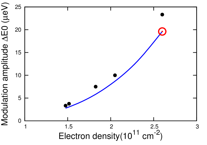
Figure 7: (Color online) Amplitude of the modulation of the $q=0$ spin-wave energy, $\Delta E_{0}=(\text{Max}E_{0}-\text{Min}E_{0})/2$, as a function of the sheet density $N_{s}$ of the electron gas in the quantum well. Black dots: experimental data. Blue line: analytical results using Eq. (6).

VI Conclusions

In this paper, we presented a detailed theoretical and experimental study of spin-wave dispersions in a 2DEG in the presence of Rashba and Dresselhaus SOC. In earlier workPerez2016 we had limited ourselves to the leading (first-order) SOC effects, which causes a momentum-dependent shift of the spin-wave dispersions, but leaves the spin-wave stiffness as well as Larmor’s theorem intact. We have now discovered some subtle corrections which arise when second-order SOC effects are taken into account: Larmor’s theorem is broken, and the spin-wave stiffness is modified. Both corrections are relatively small (of order 10% or less) but experimentally detectable.

We presented a linear-response theory, based on TDDFT, to fully account for SOC effects to first, second and higher orders in SOC. A detailed comparison with experimental data, obtained using inelastic light scattering, confirmed the accuracy of the theory and allowed us to extract the SOC parameters $\alpha$ and $\beta$, as well as the renormalized Zeeman splitting $Z^{*}$.

A major outcome of our study is that we discovered that the ALDA does not lead to a satisfactory description of the second-order SOC modulation effects of the spin waves. At present, there are only few approaches in ground-state DFT for noncollinear magnetism that go beyond the LDA, such as the optimized effective potential (OEP)Sharma2007 or gradient corrections.Scalmani2012 ; Eich2013a ; Eich2013b This provides motivation for the search for better xc functionals in TDDFT for noncollinear spins. In particular, any such new xc functional should be well-behaved in the crossover between three-and two-dimensional systems.Karimi2014

The study of spin waves in electron gases confined in semiconductor quantum wells under the presence of SOC is also of practical interest. Manipulation of the Rashba and Dresselhaus coupling strengths can be used to control the spin-wave group velocity.Perez2016 Since spin waves can be used as carriers of spin-based information, this may lead to applications in spintronics. Here we have provided a suitable theoretical framework to describe these effects.

- (1) L. D. Landau and E. M. Lifshitz, The classical theory of fields, 4th edition (Butterworth-Heinemann, Oxford, 1975).
- (2) E. Lipparini, Modern many-particle physics, 2nd edition (World Scientific, Singapore, 2008).
- (3) K. Yosida, Theory of magnetism (Springer, Berlin, 1996).
- (4) D. Stein, K. v. Klitzing, and G. Weimann, Phys. Rev. Lett. 51, 130 (1983).
- (5) J. P. Longo and C. Kallin, Phys. Rev. B 47, 4429 (1993).
- (6) M. Califano, T. Chakraborty, P. Pietiläinen, and C.-M. Hu, Phys. Rev. B 73, 113315 (2006).
- (7) Y.-T. Zhang, Z.-F. Song, and Y.-C. Li, Phys. Lett. A 373, 144 (2008).
- (8) R. Roldán, J.-N. Fuchs, and M. O. Goerbig, Phys. Rev. B 82, 205418 (2010).
- (9) S. S. Krishtopenko, Semicond. 49, 174 (2015).
- (10) S. Maiti, M. Imran, and D. L. Maslov, Phys. Rev. B 93, 045134 (2016).
- (11) C. A. Ullrich and M. E. Flatté, Phys. Rev. B 66, 205305 (2002).
- (12) C. A. Ullrich and M. E. Flatté, Phys. Rev. B 68, 235310 (2003).
- (13) F. Baboux, F. Perez, C. A. Ullrich, I. D’Amico, J. Gomez, and M. Bernard, Phys. Rev. Lett. 109, 166401 (2012).
- (14) F. Baboux, F. Perez, C. A. Ullrich, I. D’Amico, G. Karczewski, and T. Wojtowicz, Phys. Rev. B 87, 121303(R) (2013).
- (15) F. Baboux, F. Perez, C. A. Ullrich, G. Karczewski, and T. Wojtowicz, Phys. Rev. B 92, 125307 (2015).
- (16) F. Baboux, F. Perez, C. A. Ullrich, G. Karczewski, and T. Wojtowicz, Phys. Stat. Solidi RRL 10, 315 (2016).
- (17) F. Perez, F. Baboux, C. A. Ullrich, I. D’Amico, G. Vignale, G. Karczewski, and T. Wojtowicz, Phys. Rev. Lett. 117, 137204 (2016).
- (18) F. Perez, Phys. Rev. B 79, 045306 (2009)
- (19) F. Perez, J. Cibert, M. Vladimirova, and D. Scalbert, Phys. Rev. B 83, 075311 (2011).
- (20) E. K. U. Gross and W. Kohn, Phys. Rev. Lett. 55, 2850 (1985).
- (21) C. A. Ullrich, Time-dependent density-functional theory: concepts and applications (Oxford University Press, Oxford, 2012).
- (22) C. Attaccalite, S. Moroni, P. Gori-Giorgi, and G. B. Bachelet, Phys. Rev. Lett. 88, 256601 (2002).
- (23) F. Perez, C. Aku-leh, D. Richards, B. Jusserand, L. C. Smith, D. Wolverson and G. Karczewski, Phys. Rev. Lett. 99, 026403 (2007)
- (24) A. K. Rajagopal, Phys. Rev. B 17, 2980 (1978).
- (25) G. F. Giuliani and G. Vignale, Quantum Theory of the Electron Liquid (Cambridge University Press, 2005).
- (26) A. Ashrafi and D. L. Maslov, Phys. Rev. Lett. 109, 227201 (2012).
- (27) S. Maiti, V. Zyuzin, and D. L. Maslov, Phys. Rev. B 91, 035106 (2015).
- (28) S. Maiti and D. L. Maslov, Phys. Rev. Lett. 114, 156803 (2015).
- (29) J. P. Perdew and Y. Wang, Phys. Rev. B 45, 13244 (1992).
- (30) See Supplemental Material at http://…
- (31) In our numerical calculations, the Mn magnetic moments are not included, which does not affect the electronic structure and dynamics. However, we need to compensate by using a larger magnetic field (4.18 T) compared to experiment (2 T).
- (32) Note that in Ref. Perez2016, we obtained slightly different SOC parameters ( meVÅ and meVÅ) by using the ALDA for and fitting to only.
- (33) P. S. Eldridge, J. Hübner, S. Oertel, R. T. Harley, M. Henini, and M. Oestreich, Phys. Rev. B 83, 041301(R) (2011).
- (34) S. Sharma, J. K. Dewhurst, C. Ambrosch-Draxl, S. Kurth, N. Helbig, S. Pittalis, S. Shallcross, L. Nordström, and E. K. U. Gross, Phys. Rev. Lett. 98, 196405 (2007).
- (35) G. Scalmani and M. J. Frisch, J. Chem. Theor. Comput. 8, 2193 (2012).
- (36) F. G. Eich and E. K. U. Gross, Phys. Rev. Lett. 111, 156401 (2013).
- (37) F. G. Eich, S. Pittalis, and G. Vignale, Phys. Rev. B 88, 245102 (2013).
- (38) S. Karimi and C. A. Ullrich, Phys. Rev. B 90, 245304 (2014).