Pump-power-driven mode switching in a microcavity device
and its relation to Bose-Einstein condensation

Abstract

We investigate the switching of the coherent emission mode of a bimodal microcavity device, occurring when the pump power is varied. We compare experimental data to theoretical results and identify the underlying mechanism to be based on the competition between the effective gain on the one hand and the intermode kinetics on the other. When the pumping is ramped up, above a threshold the mode with the largest effective gain starts to emit coherent light, corresponding to lasing. In contrast, in the limit of strong pumping it is the intermode kinetics that determines which mode acquires a large occupation and shows coherent emission. We point out that this latter mechanism is akin to the equilibrium Bose-Einstein condensation of massive bosons. Thus, the mode switching in our microcavity device can be viewed as a minimal instance of Bose-Einstein condensation of photons. We, moreover, show that the switching from one cavity mode to the other occurs always via an intermediate phase where both modes are emitting coherent light and that it is associated with both superthermal intensity fluctuations and strong anticorrelations between both modes.

I Introduction

The development of optical cavities He et al. (2013); Vahala (2003); Kryzhanovskaya et al. (2014); Cao and Wiersig (2015) has led to (laser-)devices with an almost vanishing lasing threshold Lermer et al. (2013); Nomura et al. (2010). Bimodal (micro)lasers have been realized in various types of systems, such as ring lasers Lett et al. (1981); Mandel and Wolf (1995), vertical-cavity surface-emitting lasers Sondermann et al. (2003), its quantum-dot micropillar variant Leymann et al. (2013a, b), and 2D photonic crystal cavity lasers Zhukovsky et al. (2007). In these systems, the switching of the mode showing coherent emission Sondermann et al. (2003); Choquette et al. (1994); Sun et al. (1995); Martin-Regalado et al. (1997); Rubio et al. (2001); Ackemann and Sondermann (2001); Marconi et al. (2016) has gathered substantial interest due to potential technical applications as optical flip-flop memories, tunable sensitive switches Ge et al. (2016); Alharthi et al. (2015) and as a simple realization of non-equilibrium phase transitions Agarwal and Dattagupta (1982); Gartner and Halati (2016).

In this article, we study the switching of the coherent emission mode in bimodal micropillar lasers occurring when the pump power is ramped up. By comparing experimental data to theoretical results based on a phenomenological model, we identify the basic mechanism underlying the mode switching to be the competition between effective gain on the one hand and the intermode kinetics on the other. Namely, the mechanism that selects which of the modes shows coherent emission is found to be fundamentally different for weak pumping (just above the threshold) and in the limit of strong pumping. For weak pumping, the selected mode (i.e. the mode selected for coherent emission) is characterized by the largest effective gain and coherent emission corresponds to lasing. In contrast, for strong pumping, the selected mode depends neither on the coupling to the gain medium nor on the loss rates of both modes. Instead it is determined completely by the intermode kinetics, i.e. by processes that transfer photons from one mode to the other. We show that this mechanism is formally identical to the one leading to Bose-Einstein condensation of an ideal gas of massive bosons (i.e. with a conserved particle number) in contact with a thermal bath. Therefore, the mode switching in our system can be viewed as a minimal instance of Bose-Einstein condensation of photons.

The question, whether a system of photons (or bosonic quasiparticles) with non-conserved particle number can undergo Bose-Einstein condensation in a similar way as a thermal gas of massive bosons has raised considerable interest in the last decade. Here the problem to be overcome is to achieve a quasi-equilibrium situation, where a single mode acquires a macroscopic occupation via a thermalizing kinetics, despite the non-equilibrium nature of the system resulting from particle loss to be balanced by pumping. Beautiful experiments, showing that such a situation can indeed be achieved, have been conducted in systems of exciton-polaritons Kasprzak et al. (2006); Balili et al. (2007); Deng et al. (2010); Wertz et al. (2010); Carusotto and Ciuti (2013); Byrnes et al. (2014); Fischer et al. (2014) magnons Demokritov et al. (2006); Bunkov and Volovik (2008); Vainio et al. (2015); Fang et al. (2016), and photons in dye-filled cavities Klaers et al. (2010). While the microcavity device investigated in this article is simpler than these systems, in the sense that it is described in terms of two relevant modes only, it captures one of the most important aspects of photon condensation in a minimal fashion, namely that the condensate mode is selected not by pumping but rather by the kinetics of the photons.

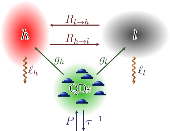
Figure 1: Illustration of the relevant processes in our bimodal system. The intermode kinetics between the modes $h$ and $l$ is determined by the rates $R_{i\to j}$. The modes lose their photons with rates $\ell_{i}$. This loss is compensated by new excitation from the quantum dots (QDs) with gain rates $g_{i}$. The quantum dots are pumped with rate $P$ and lose their excitations spontaneously with rate $\tau^{-1}$.

The starting point of our theoretical decription of a bimodal micropillar is a generic phenomenological master equation describing the relevant processes of the system Rice and Carmichael (1994); Leymann et al. (2013a): the coupling between the pumped medium and the cavity modes, loss, and the intermode kinetics (Fig. 1). Such birth-death models have also been used to study (analogs of Bose-Einstein condensation in) population dynamics Knebel et al. (2013, 2015), transport Hirschberg et al. (2009); Evans and Hanney (2005), and networks Bianconi and Barabási (2001) as well as quantum gases of massive bosons Vorberg et al. (2013, 2015). This approach, which is different from the microscopic modeling pursued in former studies of bimodal (micro) lasers Haken and Sauermann (1963); Tehrani and Mandel (1978); Mandel and Wolf (1995); Leymann et al. (2013a); Khanbekyan et al. (2015); Ge et al. (2016); Redlich et al. (2016); Fanaei et al. (2016) and interacting exciton-polariton systems, e.g., Refs. Krizhanovskii et al. (2008); Dagvadorj et al. (2015); Altman et al. (2015), provides excellent agreement with the experimental data (Fig. 2). In order to treat these equations analytically, we work out an approximation scheme that combines the theory of Bose selection, which was recently developed to describe (non-equilibrium) Bose condensation of ideal gases of massive bosons with conserved particle number Vorberg et al. (2013), with particle loss and the coupling to a pumped reservoir (gain medium). We justify this approximation by exact numerical simulations. Somewhat counter-intuitively, our theory shows that it is the limit of strong pumping, where the selected mode is determined by the intermode kinetics, which is described by terms that are formally identical to those appearing in the description of massive bosons and their equilibrium condensation. We also find that the mode switching occurs via an intermediate phase where both modes are emitting coherently (see phase diagram in Fig. 3 below).

Figure 2: Measured and calculated microcavity input-output characteristics (high-effective-gain mode in red, low-effective-gain mode in gray). The injection current $I$ is proportional to the pump rate $P$. Here, circles (connected to guide the eye), solid curves, and dashed curves refer to experimentally measured data, exact Monte-Carlo results, and asymptotic mean-field theory, respectively. Panel (a) depicts the mean occupations of the modes and the number of excited carriers (light green) in arbitrary units. The colored bars at the bottom of this panel mark the phases determined by the asymptotic theory (see Sec. IV.3). Panel (b) shows the autocorrelation $g_{ii}^{(2)}$ for both modes in comparison with the value 2 expected for thermal emission (dotted black line). Panel (c) depicts the crosscorrelation $g_{hl}^{(2)}$ in comparison to the value 1 for correlated emission (dotted black line). For the theoretical curves, we use $s=0$, $G=0.77$ as well as (in units of the spontaneous loss rate $\tau^{-1}$) $g_{h}=1.6\cdot 10^{-3}$, $g_{l}=2.1\cdot 10^{-3}$, $\ell_{h}=2.2\cdot 10^{-2}$, $\ell_{l}=3.8\cdot 10^{-2}$, $R_{l\to h}=1.7\cdot 10^{-4}$, $A_{h\to l}=8.5\cdot 10^{-6}$ (see App. A).

We investigate also the statistical properties of our system. In bimodal lasers, where one mode dominates the emission for all pump rates, the non-lasing mode exhibits usually super-thermal intensity fluctuations Lett et al. (1981); Leymann et al. (2013a) and the emission of both modes is strongly anticorrelated Lett (1986); Mandel and Wolf (1995); Roy et al. (1980); Murthy and Dattagupta (1985); Redlich et al. (2016). In the situation where mode switching occurs, we find that the super-thermal intensity fluctuations of the non-selected mode and strong anti-correlations occur whenever a mode starts or ceases to be selected. We show that these experimentally observed statistical properties can be described theoretically by an effective reduction of the spontaneous inter-mode transitions caused by mode interactions.

This paper is organized as follows. In Sec. II the experimental setup is presented. The theoretical description in terms of a master equation is introduced in Sec. III. An analytical theory of the mode switching and its relation to Bose-Einstein condensation is then worked out in Sec. IV. Finally, in Sec. V, we investigate the statistical properties of the system, before coming to the conclusions in Sec. VI.

II Experiment

Electrically-pumped quantum-dot micropillars are fabricated by etching of a planar AlAs/GaAs distributed Bragg reflector $\lambda$-cavity in which a single active layer of self-assembled In_0.3Ga_0.7As quantum dots is embedded centrally Kistner et al. (2008). A detailed description can be found in Ref. Böckler et al. (2008). The micropillar used in this study has a diameter of $3.0~{}\mu m$. Due to the strong confinement of light, the micropillars exhibit a spectrum of discrete modes. The fundamental modes $HE_{1,1}$ are composed of two orthogonally linearly polarized components, which are ideally energetically degenerate. In reality, however, asymmetries in the manufacturing process, which results in slightly elliptical structures, lift the energetical degeneracy of the fundamental modes He et al. (2013); Reitzenstein et al. (2007). The resulting mode splitting of the micropillar used in this study is $(42\pm 2)~{}\mu eV$. Besides a finite mode splitting the two fundamental modes also exhibit slightly different quality factors, $14000\pm 1500$ and $12500\pm 1500$, respectively. The different spectral and local overlaps of the modes with the gain medium and the modes polarization alters their coupling to the quantum dot emitters. As a consequence, the former mode (mode $h$) is characterized by a higher effective gain [i.e. gain-loss ratio, see Eq. (4) below] than the latter one, which has a lower effective gain (mode $l$).

A high-resolution ($25~{}\mu eV$) micro-electroluminescence setup is used to characterize the micropillars spectrally at cryogenic temperatures of $15\,K$. A linear polarizer as well as a $\lambda/4$-plate in front of the monochromator enables polarization-resolved spectroscopy. For statistical analysis via the autocorrelation function $g^{(2)}_{ii}(\tau=0)$ with zero delay time of the emission a fiber-coupled Hanbury Brown and Twiss setup is used. The temporal resolution of the Hanbury Brown and Twiss configuration based on fast Si avalanche photon diodes is $\tau_{\mathrm{res}}=40~{}ps$. For measuring the equal-time crosscorrelation function $g^{(2)}_{hl}(\tau=0)$ between the orthogonally polarized micropillar modes the emission is selected by a polarization maintaining 50/50 beamsplitter and the split beam is directed to a second identical spectrometer - with the polarizer in front of the second monochromator oriented orthogonally to the first. These equal-time correlations are defined by

$$g^{(2)}_{ij}(\tau=0)=\frac{\langle\hat{b}^{\dagger}_{i}\hat{b}^{\dagger}_{j}\hat{b}_{i}\hat{b}_{j}\rangle}{\langle\hat{b}^{\dagger}_{i}\hat{b}_{i}\rangle\langle\hat{b}^{\dagger}_{j}\hat{b}_{j}\rangle}\equiv g^{(2)}_{ij},$$ (1)

where $\hat{b}_{i}$ is the bosonic annihilator operator of mode $i$. The emission characteristics of the CW-pumped micropillar are shown in Fig. 2. In (a) the output characteristics of modes $h$ (red) and $l$ (gray) are shown as a function of the injection current $I$ (quantifying the pumping strength). Up to about $13~{}\mu A$ (phase A) both modes are below threshold and show a small increase in output emission only. Between $13~{}\mu A$ and $36~{}\mu A$ (phase B) the mode $h$ is selected and its emission increases strongly while that of mode $l$ remains small. Between $36~{}\mu A$ and $50~{}\mu A$ (phase C) both modes are selected, but while the emission intensity of mode $l$ increases that of mode $h$ decreases. Beyond $50~{}\mu A$ (phase D) only mode $l$ is selected. In Fig. 2 (b) and (c) the zero-delay autocorrelation $g_{ii}^{(2)}$ and crosscorrelation $g_{hl}^{(2)}$ functions are plotted. Note that, due to finite temporal resolution of the avalanche photodiode detectors and the low coherence time of the modes, we could not properly resolve $g_{ii}^{(2)}$ experimentally for values above $1$ in phase A and B Ulrich et al. (2007).

III Master Equation

Our starting point for the theoretical description of the system is a phenomenological master equation for the probabilities $\rho^{{\bm{n}}}_{N}$ to find the system in a state with $N$ excited emitters and photon numbers ${\bm{n}}=(n_{h},n_{l})$ in the high- and the low-effective-gain mode. It takes the form

$$\frac{\mathrm{d}}{\mathrm{d}t}\rho^{{\bm{n}}}_{N}=C_{\text{laser}}(\rho)+C_{\text{kin}}(\rho)$$ (2)

and shall be solved for the steady-state state obeying

$$\frac{\mathrm{d}}{\mathrm{d}t}\rho^{{\bm{n}}}_{N}=0.$$

The first term on the right hand side of the master equation (2) describes how photons leave and enter the cavity modes via loss and coupling to the emitters. It is given by

$$C_{\text{laser}}(\rho)= P\left[\rho^{{\bm{n}}}_{N-1}-\rho^{{\bm{n}}}_{N}\right]-\tau^{-1}[N\rho^{{\bm{n}}}_{N}-(N+1)\rho^{{\bm{n}}}_{N+1}]$$

$$-\sum_{i}g_{i}[N(n_{i}+1)\rho^{{\bm{n}}}_{N}-(N+1)n_{i}\rho^{{{\bm{n}}}-{\bf e_{i}}}_{N+1}]$$

$$-\sum_{i}\ell_{i}[n_{i}\rho^{{\bm{n}}}_{N}-(n_{i}+1)\rho^{{{\bm{n}}}+{\bf e_{i}}}_{N}],$$ (3)

where $P$ and $\tau^{-1}$ denote the pump and the loss rate of the emitters, respectively, $g_{i}$ quantifies the gain of cavity mode $i$ from the emitters, and $\ell_{i}$ is the loss rate of cavity mode $i$. An additional or removed photon in mode $i$ is denoted by $\pm{\bf e_{i}}$, [i.e., ${\bm{e}}_{h}=(1,0)$, ${\bm{e}}_{l}=(0,1)$]. The modes $h$ and $l$ are defined by the higher and lower effective gain $g_{i}/l_{i}$, respectively, so that we obtain an effective-gain ratio

$$G\equiv\frac{g_{l}/\ell_{l}}{g_{h}/\ell_{h}}<1.$$ (4)

The terms contained in $C_{\text{laser}}(\rho)$ are sufficient for a theoretical description of single-mode lasing in mode $h$ Rice and Carmichael (1994).

The second term of the master equation (2) captures the intermode kinetics and reads

$$C_{\text{kin}}(\rho)= -\sum_{i,j}R_{i\to j}\big{[}n_{i}(n_{j}+s)\rho^{{\bm{n}}}_{N}$$

$$-(n_{i}+1)(n_{j}-1+s)\rho^{{{\bm{n}}}+{\bf e_{i}}-{\bf e_{j}}}_{N}\big{]}.$$ (5)

It is characterized by the rates $R_{i\to j}$ for a transition from mode $i$ to mode $j$. The rate asymmetry of the direct intermode transitions

$$A_{i\to j}=R_{i\to j}-R_{j\to i}$$ (6)

is generally nonzero. The origin of this rate asymmetry was attributed to stimulated scattering due to carrier population oscillations, e.g., in coupled photonic crystal nanolasers Marconi et al. (2016). Furthermore asymmetric backscattering of electromagnetic waves was observed in optical microcavities Wiersig et al. (2008); Wiersig (2011); Peng et al. (2016). In our system the rate asymmetry $A_{h\to l}$ is positive,

$$A_{h\to l}>0,$$ (7)

so that the low-effective-gain mode $l$ is favored by the intermode kinetics. The parameter $s$ in Eq. (III) quantifies the ratio between spontaneous and induced intermode transitions. Its natural value is $s=1$. However, a reduction of $s$ to values $s<1$ is a simple way to effectively capture inter-mode interactions that lead to a relative enhancement of transitions into strongly occupied modes. We will show below that, while $s$ has (practically) no impact on the phase transition and the mean occupation(s) of the selected mode(s), it does affect the occupation of the non-selected mode. Only for $s<1$, the master equation can describe the experimentally observed super-thermal fluctuations $g^{(2)}_{il}>2$ of the non-selected mode. The numerical data shown in Figs. 2, 4, and 5 are obtained for $s=0$.

The form of the term $C_{\text{kin}}(\rho)$ capturing the intermode kinetics is identical to that of the master equation for an ideal gas of massive bosons in contact with an environment Vorberg et al. (2013). If such a system of massive bosons is coupled to a thermal environment characterized by the temperature $T$, the intermode rates obey $R_{j\to i}/R_{i\to j}=\exp[-\Delta_{ij}/(k_{B}T)]$ with Boltzmann constant $k_{B}$ and energy splitting $\Delta_{ij}=E_{i}-E_{j}$ between modes (single-particle states) with energy $E_{i}$. In the quantum degenerate regime of low temperature or high boson density, the system will form a Bose-Einstein condensate in the single-particle state of lowest energy. When increasing the total number of bosons $N_{B}$ in this regime, the occupation of an excited mode $i$ approaches the finite value $\langle\hat{n}_{i}\rangle=(e^{E_{i}/k_{B}T}-1)^{-1}$, while the ground-state occupation increases linearly with $N_{B}$. Even for a finite number of discrete energy levels $i$, in the limit $N_{B}\to\infty$ this behavior clearly describes Bose-Einstein condensation as the macroscopic occupation of one single-particle state (see e.g. Ref. Vorberg et al. (2015)).

The most intriguing result of this paper, shown below, is that the behavior of the bimodal system in the limit of strong pumping strength $P$ closely resembles that of a Bose-Einstein condensed gas of massive bosons in equilibrium. Remarkably here the selected mode does not depend on the effective gain, but is determined exclusively by the intermode transitions $R_{i\to j}$. This countner intuitive result is related to the fact that the intermode kinetics scales quadratically, but gain and loss only linearly with the mode occupations.

It is instructive to define the dimensionless parameter $\varepsilon$,

$$\frac{R_{l\to h}}{R_{h\to l}}\equiv\exp(-\varepsilon),$$ (8)

which can be interpreted as the ratio $\varepsilon=\Delta^{\text{eff}}_{hl}/(k_{B}T_{\text{eff}})$ of an effective energy splitting $\Delta^{\text{eff}}_{hl}$ between both modes and an effective temperature $T_{\text{eff}}$. In the limit of strong pumping, the intermode kinetics makes the photons condense into the mode corresponding to the lower effective energy. That is for $\varepsilon>0$ or $A_{h\to l}>0$ ($\varepsilon<0$ or $A_{h\to l}<0$) a Bose-Einstein condensate of photons is formed in mode $l$ (mode $h$). In contrast, it is always the mode $h$, characterized by the higher effective gain, that starts lasing when the pump power $P$ is ramped up. Thus, a rate asymmetry $A_{h\to l}>0$ implies a switching from lasing in mode $h$ to condensation in mode $l$, when the pump power is ramped up. In the following section, we derive an analytical theory, which describes this effect and establishes the analogy to equilibrium Bose-Einstein condensation for strong pumping.

IV Kinetic Theory

IV.1 Mean-field approximation

In order to obtain a closed set of kinetic equations for the mean mode occupations $\langle\hat{n}_{i}\rangle=\sum_{{\bm{n}},N}\rho_{N}^{{\bm{n}}}n_{i}$ and the mean number of excited emitters $\langle\hat{N}\rangle=\sum_{{{\bm{n}}},N}\rho_{N}^{{\bm{n}}}N$, we perform the mean-field approximation

$$\langle\hat{n}_{i}\hat{n}_{j}\rangle\approx\langle\hat{n}_{i}\rangle\langle\hat{n}_{j}\rangle\quad\text{and}\quad\langle\hat{N}\hat{n}_{i}\rangle\approx\langle\hat{N}\rangle\langle\hat{n}_{i}\rangle.$$ (9)

This approximation, which ignores non-trivial two-particle correlations, is later justified by comparing it to exact solutions of the full master equation (2) obtained from Monte-Carlo simulations (see Fig. 2). Employing it, we derive kinetic equations of motion for the mean occupations:

$$\frac{\mathrm{d}}{\mathrm{d}t}\langle\hat{n}_{i}\rangle= \sum_{j}\big{[}R_{j\to i}\langle\hat{n}_{j}\rangle(\langle\hat{n}_{i}\rangle+s)-R_{i\to j}\langle\hat{n}_{i}\rangle(\langle\hat{n}_{j}\rangle+s)\big{]}$$

$$+g_{i}\langle\hat{N}\rangle\big{(}\langle\hat{n}_{i}\rangle+1\big{)}-\ell_{i}\langle\hat{n}_{i}\rangle,$$ (10)

$$\frac{\mathrm{d}}{\mathrm{d}t}\langle\hat{N}\rangle= -\frac{\langle\hat{N}\rangle}{\tau}+P-\sum_{i}g_{i}\langle\hat{N}\rangle\big{(}\langle\hat{n}_{i}\rangle+1\big{)}.$$ (11)

IV.2 Asymptotic theory

In a next step, for the sake of finding an analytical expression for the mean occupation(s) of the selected mode(s), in Eq. (IV.1) we neglect spontaneous processes relative to corresponding stimulated ones, $(\langle\hat{n}_{i}\rangle+a)\simeq\langle\hat{n}_{i}\rangle$ with $a=1,s$. This approximation is valid asymptotically in the limit of large occupations of the emitters and the selected mode(s). Note, for high-$\beta$ cavities, where almost the entire spontaneous emission goes into the cavity modes, this assumption is plagued by the strong presence of spontaneous emission at the first threshold. Still, this assumption is valid in the coherent emission regime and, in particular, when describing transitions, where the selected modes change. Using the asymptotic approximation above, the stationary solution of Eq. (IV.1) obeys

$$\langle\hat{n}_{i}\rangle\Big{[}g_{i}\langle\hat{N}\rangle-\ell_{i}+\sum_{j}A_{j\to i}\langle\hat{n}_{j}\rangle\Big{]}=0.$$ (12)

This equation is solved by mean occupations that can be divided into two classes. For the non-selected modes $i\notin\mathcal{S}$, one finds the trivial solution $\langle\hat{n}_{i}\rangle=0$, whereas the occupations of the selected modes $i\in\mathcal{S}$ obey a linear set of equations:

$$\sum_{j\in\mathcal{S}}A_{j\to i}\langle\hat{n}_{j}\rangle =\ell_{i}-g_{i}\langle\hat{N}\rangle,\quad\forall i\in\mathcal{S}.$$ (13)

The occupation of the non-selected states, which vanishes in leading order [Eq. (12)], can be computed in the next order of our approximation. For this purpose, we take into account those terms, which are linear in the number of excited emitters $\langle\hat{N}\rangle$ or the occupations $\langle\hat{n}_{i}\rangle$ of the selected modes. We find:

$$\langle\hat{n}_{i}\rangle=\frac{g_{i}\langle\hat{N}\rangle+s\sum_{j\in\mathcal{S}}R_{j\to i}\langle\hat{n}_{j}\rangle}{\ell_{i}-g_{i}\langle\hat{N}\rangle-\sum_{j\in\mathcal{S}}A_{j\to i}\langle\hat{n}_{j}\rangle}\quad\forall i\notin\mathcal{S}.$$ (14)

The dependence of the number of excited emitters on the pumping can be obtained by analogue reasoning,

$$\langle\hat{N}\rangle=\frac{P}{\tau^{-1}+\sum_{j\in\mathcal{S}}g_{j}\langle\hat{n}_{j}\rangle}.$$ (15)

Following the strategy recently employed for massive bosons Vorberg et al. (2013), the set of selected modes $\mathcal{S}$ can now be determined by the physical requirement that all modes (both selected and non-selected modes) must have positive occupations,

$$\langle\hat{n}_{i}\rangle\geq 0\ \forall i.$$ (16)

For the non-selected modes this implies that the denominator of Eq. (14) has to be positive. Thus, the set of selected modes and their occupations are independent of the parameter $s$ since $s$ occurs neither in Eq. (13) nor in the denominator of Eq. (14).

IV.3 Phase diagram of the bimodal microcavity system

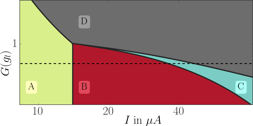
Figure 3: Phase diagram with phases (A) no selected mode, (B) mode $h$ is selected, (C) both modes are selected, and (D) mode $l$ is selected. Plotted versus the injection current $I$ that is proportional to pump rate $P$ and the ratio of the effective gain rates $G=g_{l}\ell_{h}/g_{h}\ell_{l}$ with fixed $g_{h}\ell_{l}/\ell_{h}$. Except for $g_{l}$ all parameters are the same as in Fig. 2. The dashed line indicates the value of $g_{l}$ used in Fig. 2. While for $G<1$ all phases are present when increasing the pump rate $P$, for $G>1$ the mode $l$, that is favored by the direct mode coupling becomes actually the high-effective-gain mode so that no mode switching occurs.

Based on the asymptotic theory, we can now compute the non-equilibrium phase diagram. The concept of selected modes, which appeared naturally in the asymptotic theory, clearly separates the parameter space into different phases, where no, one, or both modes are selected. A transition, where one of the non-selected modes becomes selected and starts emitting coherent light, is indicated by the divergence of its occupation described by Eq. (14). In turn, a selected mode ceases to be selected when its occupation, obtained by solving Eq. (13), drops to zero. In this section we will use this argument to compute the phase boundaries analytically. The resulting phase diagram is depicted in Fig. 3.

In phase A, for small pumping power $P$, neither mode is selected, $\mathcal{S}=\{\}$. According to Eq. (14) the mode occupations read

$$\langle\hat{n}_{i}\rangle_{A}\approx\frac{1}{\ell_{i}/(g_{i}\langle\hat{N}\rangle)-1}\ ,$$ (17)

and the number of excited emitters increases linearly with the pump rate,

$$\langle\hat{N}\rangle_{A}=\tau P.$$ (18)

When the pumping is increased and reaches

$$P_{AB}\approx\frac{\ell_{h}}{g_{h}\tau},$$ (19)

the occupation of the high-effective-gain mode diverges indicating the transition to a regime where this mode is selected and starts emitting coherently (see Eq. (14)). Since before the transition no mode is selected yet, this asymptotic estimate for the critical pumping strength cannot be expected to mark precisely the threshold in the high-$\beta$ limit. Note, however, that the estimates for further thresholds at $P_{BC}$ and $P_{CD}$ are not plagued by this problem, since they occur in the regime where at least one mode is selected already.

In phase B the high-effective-gain mode is selected, $\mathcal{S}=\{h\}$, and the number of excited emitters is clamped at the threshold value [see Eq. (13) and Fig. 2 (a)]

$$\langle\hat{N}\rangle_{B}=\frac{\ell_{h}}{g_{h}}.$$ (20)

The excitation provided by increasing the pumping is directly transferred to the selected mode Siegman (1986). Consequently, the occupation of the selected high-effective-gain mode depends linearly on the pump rate [use Eq. (15)]

$$\langle\hat{n}_{h}\rangle_{B}=\frac{P}{\ell_{h}}-\frac{1}{\tau g_{h}}.$$ (21)

The occupation in the non-selected low-effective-gain mode is given by [see Eq. (14)]

$$\langle\hat{n}_{l}\rangle_{B}=\frac{g_{l}\langle\hat{N}\rangle_{B}+sR_{h\to l}\langle\hat{n}_{h}\rangle_{B}}{\ell_{l}-g_{l}\langle\hat{N}\rangle_{B}-A_{h\to l}\langle\hat{n}_{h}\rangle_{B}}.$$ (22)

In a case where the mode-coupling rates would favor the high-effective-gain mode $(A_{h\to l}<0)$, Eq. (22) would be valid for all pumping powers $P>P_{AB}$. However, in our case, where the mode-coupling rates favor the low-effective-gain mode $(A_{h\to l}>0)$, increasing the pump rate (and with it also $\langle\hat{n}_{h}\rangle_{B}$), eventually leads to the divergence of the right-hand side of Eq. (22). This occurs at the pump rate

$$P_{BC}=\frac{\ell_{h}}{g_{h}}\left[\frac{1}{\tau}+\frac{1}{A_{h\to l}}(g_{h}\ell_{l}-g_{l}\ell_{h})\right]$$ (23)

and indicates the transition to phase C.

In phase C both modes are selected, $\mathcal{S}=\{h,l\}$. The number of excited emitters increases again linearly with the pump rate $P$,

$$\langle\hat{N}\rangle_{C}=P\left[\frac{1}{\tau}+\frac{1}{A_{h\to l}}(g_{h}\ell_{l}-g_{l}\ell_{h})\right]^{-1}.$$ (24)

The occupations of the high- and low-effective-gain mode de- and increase linearly with $\langle\hat{N}\rangle_{C}$, respectively,

$$\langle\hat{n}_{h}\rangle_{C} =-\frac{g_{l}\langle\hat{N}\rangle_{C}-\ell_{l}}{A_{h\to l}},$$ (25)

$$\langle\hat{n}_{l}\rangle_{C} =\frac{g_{h}\langle\hat{N}\rangle_{C}-\ell_{h}}{A_{h\to l}}.$$ (26)

When the number of the emitters $\langle\hat{N}\rangle_{C}$ reaches $\ell_{l}/g_{l}$, the occupation $\langle\hat{n}_{h}\rangle_{C}$ becomes zero, indicating the transition to the phase where this mode is no longer selected. The threshold pump rate $P_{CD}$ can be obtained from Eq. (24) analogously to the expression for $P_{BC}$ and reads

$$P_{CD}=\frac{P_{BC}}{G}.$$ (27)

Thus the extent of phase C is determined by the inverse effective gain ratio $G$ [Eq. (4)].

In phase D, only mode $l$ is selected, $\mathcal{S}=\{l\}$. The number of excited emitters remains at the higher threshold value

$$\langle\hat{N}\rangle_{D}=\frac{\ell_{l}}{g_{l}},$$ (28)

and the occupation of the selected mode $l$ reads

$$\langle\hat{n}_{l}\rangle_{D}=\frac{P}{\ell_{l}}-\frac{1}{\tau g_{l}}.$$ (29)

The occupation of the non-selected mode $h$ is given by

$$\langle\hat{n}_{h}\rangle_{D}=\frac{g_{h}\langle\hat{N}\rangle_{D}+sR_{l\to h}\langle\hat{n}_{l}\rangle_{D}}{\ell_{h}-g_{h}\langle\hat{N}\rangle_{D}+A_{h\to l}\langle\hat{n}_{l}\rangle_{D}}.$$ (30)

The crucial difference to Eq. (22) is that for $A_{h\to l}>0$ an increase of $\langle\hat{n}_{l}\rangle_{D}$ cannot produce a further root in the denominator of Eq. (30). Thus no further transition will occur [unless other parameters change as well when the pump power is ramped up].

Figure 3 shows the phase diagram resulting from the asymptotic theory with respect to the effective-gain ratio $G$ (varied by varying the gain rate $g_{l}$) and the pumping strength $P$ (proportional to the injection current $I$). While the precise shape of the phase boundaries depends on the parameters (and which of them are varied in order to modify the effective-gain ratio $G$), the topology of the phase diagram is generic. For $G<1$ (and $A_{h\to l}>0$), the system always undergoes a sequence of three transitions between the phases A, B, C, D when the pump rate is increased. For $G>1$ (and $A_{h\to l}>0$), where the mode labeled $l$ actually becomes the high effective gain mode, only a single transition from phase A to phase D occurs. In summary, when the pump power $P$ is ramped up, the system starts lasing in the mode characterized by the higher effective gain, whereas in the limit of strong pumping the selected mode is the one favored by the intermode kinetics. Moreover, the switching from selection of mode $h$ to selection of mode $l$ has to occur via an intermediate phase, where both modes are selected (unless the system is fine-tuned to $G=1$).

The data plotted in Fig. 2 corresponds to a cut through this phase diagram following the dashed horizontal line in Fig. 3. The different phases obtained from the asymptotic theory are indicated by the colors at the bottom of panel (a). In Fig. 2(a), we can clearly see that the mean occupations obtained from the asymptotic theory (dashed lines) nicely reproduce the exact solution (solid line) of the master equation (2), which was obtained by Monte-Carlo simulations (for a detailed description of the method see Ref. Vorberg et al. (2015)). This agreement justifies both the mean-field approximation and the asymptotic theory. More importantly, the theoretical curves also describe the experimental data (circles in Fig. 2) very well. In appendix A we explain how the parameters of our model are determined.

IV.4 Relation to Bose-Einstein condensation

We have seen that in the limit of strong pumping strength $P$ the selected mode is determined exclusively by the intermode kinetics, which is described by the rates $R_{i\to j}$. It is remarkable that in this limit neither the loss rates of the modes $\ell_{i}$ nor their coupling $g_{i}$ to the emitters influences the selection of the mode. This counter-intuitive result is related to the fact that gain and loss scale only linearly with the mode occupations, whereas the rates for the intermode kinetics have a quadratic dependence on the mode occupations. It implies that the mechanism leading to a macroscopic (or large) occupation of one of the modes is the same as the one that leads to the Bose-Einstein condensation of massive bosons in contact with a thermal environment. This is based on Bose-enhanced inter-mode kinetics (scattering) described, e.g., in Ref. Vorberg et al. (2013) on the basis of a rate equation comprising the same terms as $C_{\text{kin}}$ [Eq. (III)].

Even though the system consists of two levels only, the notion of Bose condensation becomes sharp in the limit $P\to\infty$, where the occupation of mode $l$, given by Eq. (29), approaches infinity, while that of mode $h$, given by Eq. (30), remains below a finite value. Note that also the number of excited emitters, given by Eq. (28), remains at a finite value in this limit. This has the important consequence that the occupation of the non-condensed mode $h$ is determined completely by the intermode kinetics described by the rates $R_{i\to j}$. In the limit $P\to\infty$ it approaches

$$\langle\hat{n}_{h}\rangle\simeq\frac{s}{\exp(\varepsilon)-1},$$ (31)

where $\varepsilon$ is the parameter defined in Eq. (8). Thus, for $s=1$ the occupation of mode $l$ precisely corresponds to that of an excited state of energy $\varepsilon k_{B}T$ in a Bose condensed system of massive bosons at temperature $T$. The fact that the “excited-state” occupation $\langle\hat{n}_{h}\rangle$ (the depletion) approaches a constant value for strong pumping, so that increasing the number of photons (bosons) in the system will only increase the condensate occupation, is another clear analogy to equilibrium Bose condensation. Irrespective of the value of $s$, for strong pumping the selection of the coherent emission mode is a result of the intermode kinetics.

V Photon statistics

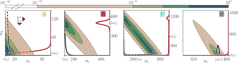
Figure 4: Two-mode photon statistics obtained from the reduced master equation (see Appendix 7) with single-mode statistics for mode $l$ at the bottom (black) and mode $h$ at the right (red) axis, for injection currents $I=12.5\,\mu A,27.4\,\mu A,41.7\,\mu A,60\,\mu A$ (phase A, B, C, D). These pump rates are also indicated by arrows in Fig. 2(b). The labels $\langle\hat{n}_{h}\rangle$ and $\langle\hat{n}_{l}\rangle$ mark the position of the expectation value for each mode. For a better comparison the single-mode statistics are depicted up to $0.025$% in solid lines, while the remaining part is dashed. Note that plotted range of photon numbers increases from left to right.

In microlasers, where almost the entire spontaneous emission goes into a single mode, no sharp intensity jump is visible at the lasing threshold Rice and Carmichael (1994); Lermer et al. (2013). Instead the transition to coherent emission is indicated in the autocorrelation Glauber (1963) of the emitted photons Strauf et al. (2006); Ulrich et al. (2007); Wiersig et al. (2009); Aßmann et al. (2009); Leymann et al. (2014); Chow et al. (2014); Jin et al. (1994). To confirm the coherence properties of the emitted photons, we examine the photon statistics. The equal-time photon correlation functions (1), which we can write like

$$g^{(2)}_{ij}=\begin{cases}\big{(}\langle\hat{n}_{i}\hat{n}_{i}\rangle-\langle\hat{n}_{i}\rangle\big{)}/\langle\hat{n}_{i}\rangle^{2}&\mbox{ if }i=j\\ \langle\hat{n}_{i}\hat{n}_{j}\rangle/\langle\hat{n}_{i}\rangle\langle\hat{n}_{j}\rangle&\mbox{ if }i\neq j~{},\end{cases}$$ (32)

measure the occupation number fluctuations of each mode and the crosscorrelation between the modes, respectively. In Fig. 2 (b) and (c) experimental and theoretical results for $g^{(2)}_{ii}$ and $g^{(2)}_{hl}$ are depicted. The theoretical values for $g^{(2)}_{ij}$ are determined by a numerically exact Monte-Carlo simulation of the full master equation (2). As discussed above a change from $g^{(2)}_{hh}=2$ to $g^{(2)}_{hh}=1$ indicates the first threshold where the coherent emission in mode $h$ sets in, as can be seen clearly in Fig. 2. For even stronger pumping, when entering or leaving phase $C$, in which both modes are selected, we observe pronounced anticorrelations between both modes ($g_{hl}<1$) as well as superthermal intensity flucutations ($g_{ii}>2$) of that mode $i$ that changes its state from non-selected to selected or vice versa. Note that for our system parameters, phase C appears in a narrow interval of pump powers only so that its properties are overshadowed by those of the transitions BC and CD. As a result, the two minima of the crosscorrelations occurring at the transitions have merged to a single one.

In order to reproduce the measured superthermal intensity fluctuations at the transitions BC and CD theoretically, we have to choose $s<1$, corresponding to the presence of intermode interactions. The best results are obtained for the value $s=0$, which we used also in the simulations (the role of $s$ will be discussed in more detail below and in Appendix C).

We will now investigate the signatures of the mode switching in the reduced two-mode photon distribution $\rho^{n_{h},n_{l}}=\sum_{N}\rho^{n_{h},n_{l}}_{N}$, which gives the probability to find the system in a state with $n_{h}$ and $n_{l}$ photons in mode $h$ and mode $l$, respectively. We compute this quantity by solving either the full master equation (phases A and B) or the reduced master equation for $\rho^{n_{h},n_{l}}$ (phases C and D, see Appendix 7 for details). Results for four different pump powers $P$, corresponding to the four phases A to D, are depicted in Fig. 4. The corresponding single-mode distributions $\rho^{n_{h}}=\sum_{n_{l}}\rho^{n_{h},n_{l}}$ and $\rho^{n_{l}}$ are shown as well.

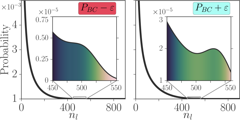
Figure 5: Photon statistics of mode $l$ ($\rho^{n_{l}}$) for pump rates below ($P_{BC}-\varepsilon$, left panel) and above ($P_{BC}+\varepsilon$, right panel) with $\varepsilon=0.016\mu A$. Only in the right panel the photon statistics exhibits a second local maximum. The system parameters are the same as in Fig. 2.

In the non-selected phase A the distribution possesses a single maximum at ${\bm{n}}=(n_{h},n_{l})=(0,0)$. The selection of mode $h$ (phases B and C) is associated with a maximum of the distribution at ${\bm{n}}=(n^{\text{max}}_{h},0)$ lying on the vertical axis, whereas the selection of mode $l$ (phases C and D) with a maximum at ${\bm{n}}=(0,n^{\text{max}}_{l})$ lying on the horizontal axis. Thus, in phase $C$ where both modes are selected, the distribution possesses two local maxima that are separated by a saddle point . The emergence of the second maximum when entering phase $C$, is visible also in the occupation distribution of the mode that starts emitting coherently, as can be seen in Fig. 5 showing $\rho^{n_{l}}$ directly before and after the transition from $B$ to $C$. The build-up and later the presence of the second maximum in $\rho^{n_{l}}$ is accompanied by the strong (superthermal) number fluctuations in this mode.

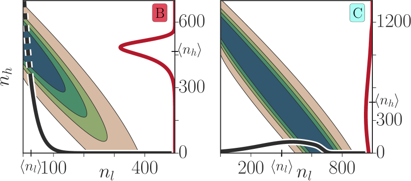
Figure 6: Two-mode photon statistics obtained from the reduced master equation for the same parameters as in Fig. 4 B and C but with fully included spontaneous transitions between the modes. In contrast to the case with suppressed spontaneous transitions, the statistics are no longer attracted to the axis. The colorbar is the same as in Fig. 4. For a better comparison the single-mode statistics are depicted up to $0.015$% in solid lines, while the remaining part is dashed.

The impact of the effective parameter $s$ is illustrated in Fig. 6, where the two-mode distribution is shown for $s=1$ in phases $B$ and $C$ for the same parameters used in the corresponding panels in Fig. 4. For $s=1$ states with zero occupation in one of the modes (situated along the axes of the plot) are much less attractive than for the value $s=0$ considered before. As a striking consequence, the selection of both modes in phase C is not associated with two maxima in the distribution anymore, but rather with a single central maximum. The transition from phase B to phase C now corresponds to the shifting of the single maximum away from the horizontal axis. As a result, for $s=1$ the system does not show the experimentally observed superthermal photon number fluctuations, as we discuss in more detail in Appendix  C. It is an interesting observation that neglecting or taking into account the spontaneous emission between the modes has such a strong impact on the statistical properties of the modeled bimodal system. Note, however, that despite this strong impact on the statistics, the mean occupations of the modes and the critical parameters for the phase transition do not show a strong dependence on $s$. This is also the result predicted by the asymptotic theory presented in the previous section.

VI Conclusion

In this paper we investigated the pump-power driven mode switching in a bimodal microcavity. We presented experimental results and their explanation in terms of a transparent analytical theory. In particular we found that the transition has to occur via an intermediate phase where both modes are selected. Our theoretical description reveals, moreover, a close connection to the physics of equilibrium Bose-Einstein condensation in quantum gases of massive bosons. The mode switching can, therefore, be viewed as a minimal instance of Bose-Einstein condensation of photons and its demarcation to lasing.

We also investigated the statistical properties of the system and pointed out that the mode switching is accompanied by superthermal intensity fluctuations as well as anticorrelations between both modes. This observation can be technically relevant, since a device producing a drastically increased occurrence rate of photon pairs (with a very narrow linewidth Khanbekyan et al. (2015)) could be used to enhance two-photon excitation process used in fluorescence microscopy Jechow et al. (2013). Furthermore a device that changes its predominantly emitting mode in dependence of the injection current could be applied for optical memories and other types of mode management Zhukovsky et al. (2007); Lv et al. (2014).

Appendix A Extracting system parameters from the measured data

The asymptotic theory describes the generic form of the mode switching and its analytic expressions can thus be used to obtain the parameters of the master equation model. However, the theoretical parameters cannot be related directly to experimental parameters due to the unknown proportionality factor $a_{i}$ between the intensity of the emitted light $J_{i}$ and the occupation of modes, $\langle\hat{n}_{i}\rangle=a_{i}J_{i}$, and the unknown excitation efficiency $b$ of the pumping with respect to the injection current, $P=bI$.

The main properties of the switching are captured by the effective-gain ratio $G$ which determines whether a switching occurs and the extent of phase C, $\frac{P_{CD}}{P_{BC}}=G^{-1}$ [see Eq. (27)]. This ratio can be obtained in the following way: Apply first a linear fit for the intensities of the selected modes $i$ in each of the phases B, C, D,

$$J_{i}(I)|_{R}=A_{iR}I+B_{iR}.$$ (33)

The ratio $\frac{P_{CD}}{P_{BC}}=\frac{I_{CD}}{I_{BC}}$ is then determined either by the intersections of $J_{h}|_{B}(I_{BC})=J_{h}|_{C}(I_{BC})$ and $J_{l}|_{C}(I_{CD})=J_{l}|_{D}(I_{CD})$ or via the points where the occupation of the modes approach zero $J_{h}|_{C}(I_{CD})=0$ and $J_{l}|_{C}(I_{BC})=0$. Both procedures give similar values for the effective-gain ratio $G$ via Eq. (27), namely 1.22 and 1.27, respectively. Thus determining $G$ does not require the knowledge of the excitation efficiency $b$ and the absolute number of cavity photons via $a_{i}$.

The parameters $A_{h\to l}$, $g_{h}$, $g_{l}$, $\ell_{h}$, $\ell_{l}$, are extracted for comparison between theory and experiment via the least squares method for all experimental data with $I<80~{}\mu A$ and are listed in the caption of Fig. 2. Since the time scale in Eq. (2) does not affect steady state properties, all parameters are measured in units of $\tau$. The individual rates $R_{l\to h}$ and $R_{h\to l}$ do not affect the asymptotic theory, only the rate asymmetry $A_{l\to h}$ does [as discussed above]. But the correlation function $g^{(2)}_{ll}$ does depend on the individual rates, so that $R_{l\to h}$ is chosen to reproduce this correlation function.

In the experiment the orientation of a polarization filter is chosen parallel to the passive cavity modes at the inversion point. Due to the interactions induced by the common gain medium the polarization-resolved spectrum exhibits a double peak structure, indicating that each polarization direction contains small portions of the other mode Khanbekyan et al. (2015). To make numerical and experimental fluctuations comparable we take into account that in each polarization a small fraction of the other mode is detected by introducing the mixing

$$n^{\mathrm{meas}}_{h,l}=(1-c)\,n_{h,l}\pm c\,n_{l,h},$$ (34)

where $n^{\mathrm{meas}}_{h,l}$ denotes the quantity that is measured. The mode mixing prevents the experimental observed fluctuations of the non-selected mode from increasing monotonically in phase D [see Fig. 2(b)]. Comparing the theoretical results with the experimental data, we find the optimal value of the mixing parameter to be very small, $c=8\cdot 10^{-3}$. Its impact of the mixing is negligible in phases A, B, and C. It is taken into account in the numerical data presented in Figs. 2 and 8, where the index ‘$\mathrm{meas}$’ is dropped.

Appendix B Reduced density matrix

Figure 7: Comparison of $\langle n_{i}\rangle$ and $g^{(2)}_{ij}$ obtained from the numerical exact Monte-Carlo simulation of Eq. (2) (solid lines) with the ones obtained from the direct solution of the reduced density matrix Eq. (35) (dashed lines). Note that the pump in the reduced density matrix is scaled to compensate that $\beta\neq 1$.

Under the (idealizing) assumption that all spontaneous emission goes into the selected modes i.e. $\tau^{-1}=0$ and $\beta=1$ a reduced density matrix of the form $\rho^{n_{h},n_{l}}$ can be derived. To derive the equation of motion for the reduced density matrix we need to consider only the parts of Eq. (2) describing the pump and the photon emission into the cavity

$$\frac{\mathrm{d}}{\mathrm{d}t}\rho^{{{\bm{n}}}}_{N}=+ P\left[\rho^{{{\bm{n}}}}_{N-1}-\rho^{{{\bm{n}}}}_{N}\right]+[\dots]$$ (35)

$$- \sum_{i}g_{i}[N(n_{i}+1)\rho^{{\bm{n}}}_{N}-(N+1)n_{i}\rho^{{{\bm{n}}}-{\bf e_{i}}}_{N+1}].$$

Here and in the following equation $[\dots]$ stands for terms that describe describe the loss of the individual modes as well as intermode transitions. When no spontaneous emission is lost into non-selected modes the carrier recombination and emission into the cavity modes is faster than any other process so that the term ${\sum_{i}g_{i}N(n_{i}+1)\rho^{{\bm{n}}}_{N}}$ can be substituted by $P\rho^{{\bm{n}}}_{N-1}$. This means that whenever an emitter is excited by the pump its excitation is immediately emitted into the cavity, thus the emission into the modes can be described directly by $P\rho^{{\bm{n}}}_{N-1}$ Rice and Carmichael (1994). By the same reasoning or by simply shifting the indices (${\rho^{{\bm{n}}-{\bf e_{i}}}_{N+1}}$) one can find a substitute for all terms in Eq. (2) that correspond to the photon emission. Now we can trace over the emitter subspace ($\sum_{N}$), resulting in an equation of motion for the reduced density matrix,

$$\frac{\mathrm{d}}{\mathrm{d}t}\rho^{{{\bm{n}}}}=- P\rho^{{{\bm{n}}}}+\sum_{i}\frac{P\,g_{i}n_{i}\rho^{{\bm{n}}-{\bf e_{i}}}}{\sum_{j}g_{j}(n_{j}+1)-g_{i}}+[\dots].$$

As argued above, the reduced density matrix approach works under the assumption of $\beta=1$. In our case $\beta\simeq 0.2$, so only a fraction of the pump effectively creates photons in the cavity. To be able to compare the reduced density matrix to the full model the pump power is scaled accordingly. Figure 7 shows the results of the Monte-Carlo simulations of the full equation compared to the results obtained from numerical solution of the reduced equation. The deviation of the reduced density matrix approach for small pump rates is not a problem since for low pump rates the full equation can still be solved numerically exactly (as it is done for Fig. 4 A and B). Importantly, the reduced equation reproduces the results in the regime of high pump rates, where the exact solution for the full equation can no longer be obtained.

Appendix C The role of spontaneous intermode transitions

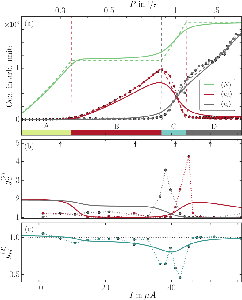
Figure 8: Calculated input-output characteristics and fluctuation for both modes in the presence of spontaneous transitions between the modes, $s=1$. The fluctuation are restricted to values $g^{(2)}_{ii}\leq 2$. All parameters are chosen as in Fig. 2.

In this appendix we investigate the impact of the effective parameter $s$, which quantifies spontaneous intermode transitions. Figure 8 shows the mode characteristics for the case with full spontaneous transitions between the modes ($s=1$). In contrast to Fig. 2, the sharp kinks in the occupations [panel (a)] and the cross correlation [panel (c)] in phase C are less pronounced. However, the most significant deviation appears in the photon autocorrelations. For $s=1$ the computed autocorrelation does not reproduce the experimentally observed superthermal fluctuations, $g^{(2)}\leq 2$.

This numerical observation can be backed analytically using the following argument. In phase B and D the joint distribution $\rho^{{{\bm{n}}}}_{N}$ factorizes approximately into two parts, one describing the non-selected mode $i$ and the other one describing the selected mode $j$ and the emitters, $\rho^{{{\bm{n}}}}_{N}\approx\rho^{n_{i}}\rho^{n_{j}}_{N}$. This statement is confirmed by the numerical solution of the full master equation. Such a factorization allows one, to trace out both the selected mode and the emitters, to obtain an equation of motion for the photon number distribution of the non-selected mode:

$$\frac{\mathrm{d}}{\mathrm{d}t}\rho^{n} =-\langle\hat{N}\rangle g[(n+1)\rho^{n}-n\rho^{n-1}]$$

$$- \ell[n\rho^{n}-(n+1)\rho^{n+1}]$$

$$- R_{j\to i}\langle\hat{n}_{j}\rangle\big{[}(n+s)\rho^{n}-(n-1+s)\rho^{n-1}\big{]}$$

$$- R_{i\to j}(\langle\hat{n}_{j}\rangle+s)\big{[}n\rho^{n}-(n+1)\rho^{n+1}\big{]}.$$ (36)

Here, $n$ denotes the photon number of the non-selected mode, $\langle\hat{n}_{j}\rangle,\langle\hat{N}\rangle$ the mean occupations of the selected mode and the emitters respectively, $R_{j\to i}(R_{i\to j})$ the transition rate from (to) the selected mode $j$ to (from) the non-selected mode, and $g$, $\ell$ the gain and loss rate of the non selected mode. If spontaneous transitions are fully included, $s=1$, Eq. (36) is solved by a distribution of the form $\rho^{n}=(1-\alpha)\alpha^{n}$, which always yields $g^{(2)}=2$. This explains why we do not find superthermal fluctuations for $s=1$.

References

- He et al. (2013) Lina He, Şahin Kaya Özdemir, and Lan Yang, “Whispering gallery microcavity lasers,” Laser Photon. Rev. 7, 60–82 (2013).
- Vahala (2003) Kerry J. Vahala, “Optical microcavities,” Nature 424, 839–846 (2003).
- Kryzhanovskaya et al. (2014) N. V. Kryzhanovskaya, M. V. Maximov, and A. E. Zhukov, “Whispering-gallery mode microcavity quantum-dot lasers,” Quantum Electron. 44, 189 (2014).
- Cao and Wiersig (2015) Hui Cao and Jan Wiersig, “Dielectric microcavities: Model systems for wave chaos and non-Hermitian physics,” Rev. Mod. Phys. 87, 61–111 (2015).
- Lermer et al. (2013) M. Lermer, N. Gregersen, M. Lorke, E. Schild, P. Gold, J. Mørk, C. Schneider, A. Forchel, S. Reitzenstein, S. Höfling, and M. Kamp, “High beta lasing in micropillar cavities with adiabatic layer design,” Appl. Phys. Lett. 102, 052114 (2013).
- Nomura et al. (2010) Masahiro Nomura, Naoto Kumagai, Satoshi Iwamoto, Yasutomo Ota, and Yasuhiko Arakawa, “Laser oscillation in a strongly coupled single-quantum-dot–nanocavity system,” Nature Phys. 6, 279–283 (2010).
- Lett et al. (1981) P. Lett, W. Christian, Surendra Singh, and L. Mandel, “Macroscopic Quantum Fluctuations and First-Order Phase Transition in a Laser,” Phys. Rev. Lett. 47, 1892–1895 (1981).
- Mandel and Wolf (1995) Leonard Mandel and Emil Wolf, Optical Coherence and Quantum Optics (Cambridge University Press, 1995).
- Sondermann et al. (2003) M. Sondermann, M. Weinkath, T. Ackemann, J. Mulet, and S. Balle, “Two-frequency emission and polarization dynamics at lasing threshold in vertical-cavity surface-emitting lasers,” Phys. Rev. A 68, 033822 (2003).
- Leymann et al. (2013a) H. A. M. Leymann, C. Hopfmann, F. Albert, A. Foerster, M. Khanbekyan, C. Schneider, S. Höfling, A. Forchel, M. Kamp, J. Wiersig, and S. Reitzenstein, “Intensity fluctuations in bimodal micropillar lasers enhanced by quantum-dot gain competition,” Phys. Rev. A 87, 053819 (2013a).
- Leymann et al. (2013b) Heinrich A. M. Leymann, Alexander Foerster, Mikayel Khanbekyan, and Jan Wiersig, “Strong photon bunching in a quantum-dot-based two-mode microcavity laser,” Phys. Status Solidi B 250, 1777–1780 (2013b).
- Zhukovsky et al. (2007) Sergei V. Zhukovsky, Dmitry N. Chigrin, Andrei V. Lavrinenko, and Johann Kroha, “Switchable Lasing in Multimode Microcavities,” Phys. Rev. Lett. 99, 073902 (2007).
- Choquette et al. (1994) Kent D Choquette, DA Richie, and RE Leibenguth, “Temperature dependence of gain-guided vertical-cavity surface emitting laser polarization,” Appl. Phys. Lett. 64, 2062–2064 (1994).
- Sun et al. (1995) Decai Sun, Elias Towe, Paul H Ostdiek, Jeffery W Grantham, and Gregory J Vansuch, “Polarization control of vertical-cavity surface-emitting lasers through use of an anisotropic gain distribution in [110]-oriented strained quantum-well structures,” IEEE J. Sel. Top. Quantum Electron. 1, 674–680 (1995).
- Martin-Regalado et al. (1997) J Martin-Regalado, JLA Chilla, JJ Rocca, and P Brusenbach, “Polarization switching in vertical-cavity surface emitting lasers observed at constant active region temperature,” Appl. Phys. Lett. 70, 3350–3352 (1997).
- Rubio et al. (2001) Jaime Rubio, Loren Pfeiffer, Marzena H Szymanska, Aron Pinczuk, Song He, Harold U Baranger, Peter B Littlewood, Ken W West, and Brian S Dennis, “Coexistence of excitonic lasing with electron–hole plasma spontaneous emission in one-dimensional semiconductor structures,” Solid State Communications 120, 423–427 (2001).
- Ackemann and Sondermann (2001) T Ackemann and M Sondermann, “Characteristics of polarization switching from the low to the high frequency mode in vertical-cavity surface-emitting lasers,” Appl. Phys. Lett. 78, 3574–3576 (2001).
- Marconi et al. (2016) M. Marconi, J. Javaloyes, F. Raineri, J. A. Levenson, and A. M. Yacomotti, “Asymmetric mode scattering in strongly coupled photonic crystal nanolasers,” Opt. Lett. 41, 5628–5631 (2016).
- Ge et al. (2016) Li Ge, David Liu, Alexander Cerjan, Stefan Rotter, Hui Cao, Steven G. Johnson, Hakan E. Türeci, and A. Douglas Stone, “Interaction-induced mode switching in steady-state microlasers,” Opt. Express 24, 41 (2016).
- Alharthi et al. (2015) S. S. Alharthi, A. Hurtado, V.-M. Korpijarvi, M. Guina, I. D. Henning, and M. J. Adams, “Circular polarization switching and bistability in an optically injected 1300 nm spin-vertical cavity surface emitting laser,” Appl. Phys. Lett. 106, 021117 (2015).
- Agarwal and Dattagupta (1982) G. S. Agarwal and S. Dattagupta, “Higher-order phase transitions in systems far from equilibrium: Multicritical points in two-mode lasers,” Phys. Rev. A 26, 880–887 (1982).
- Gartner and Halati (2016) P. Gartner and C. M. Halati, “Laser transition in the thermodynamic limit for identical emitters in a cavity,” Phys. Rev. A 93, 013817 (2016).
- Kasprzak et al. (2006) J. Kasprzak, M. Richard, S. Kundermann, A. Baas, P. Jeambrun, J. M. J. Keeling, F. M. Marchetti, M. H. Szymanska, R. Andre, J. L. Staehli, V. Savona, P. B. Littlewood, B. Deveaud, and Le Si Dang, “Bose–einstein condensation of exciton polaritons,” Nature 443, 409–414 (2006).
- Balili et al. (2007) R. Balili, V. Hartwell, D. Snoke, L. Pfeiffer, and K. West, “Bose-Einstein Condensation of Microcavity Polaritons in a Trap,” Science 316, 1007–1010 (2007).
- Deng et al. (2010) Hui Deng, Hartmut Haug, and Yoshihisa Yamamoto, “Exciton-polariton bose-einstein condensation,” Rev. Mod. Phys. 82, 1489–1537 (2010).
- Wertz et al. (2010) E. Wertz, L. Ferrier, D. D. Solnyshkov, R. Johne, D. Sanvitto, A. Lemaître, I. Sagnes, R. Grousson, A. V. Kavokin, P. Senellart, G. Malpuech, and J. Bloch, “Spontaneous formation and optical manipulation of extended polariton condensates,” Nature Phys. 6, 860–864 (2010).
- Carusotto and Ciuti (2013) Iacopo Carusotto and Cristiano Ciuti, “Quantum fluids of light,” Rev. Mod. Phys. 85, 299 (2013).
- Byrnes et al. (2014) Tim Byrnes, Na Young Kim, and Yoshihisa Yamamoto, “Exciton-polariton condensates,” Nature Phys. 10, 803–813 (2014).
- Fischer et al. (2014) J. Fischer, I. G. Savenko, M. D. Fraser, S. Holzinger, S. Brodbeck, M. Kamp, I. A. Shelykh, C. Schneider, and S. Höfling, “Spatial Coherence Properties of One Dimensional Exciton-Polariton Condensates,” Phys. Rev. Lett. 113, 203902 (2014).
- Demokritov et al. (2006) S. O. Demokritov, V. E. Demidov, O. Dzyapko, G. A. Melkov, A. A. Serga, B. Hillebrands, and A. N. Slavin, “Bose–einstein condensation of quasi-equilibrium magnons at room temperature under pumping,” Nature 443, 430–433 (2006).
- Bunkov and Volovik (2008) Yuriy M. Bunkov and Grigory E. Volovik, “Bose-einstein condensation of magnons in superfluid 3he,” J. Low Temp. Phys. 150, 135–144 (2008).
- Vainio et al. (2015) O. Vainio, J. Ahokas, J. Järvinen, L. Lehtonen, S. Novotny, S. Sheludiakov, K.-A. Suominen, S. Vasiliev, D. Zvezdov, V. V. Khmelenko, and D. M. Lee, “Bose-einstein condensation of magnons in atomic hydrogen gas,” Phys. Rev. Lett. 114, 125304 (2015).
- Fang et al. (2016) Fang Fang, Ryan Olf, Shun Wu, Holger Kadau, and Dan M. Stamper-Kurn, “Condensing magnons in a degenerate ferromagnetic spinor bose gas,” Phys. Rev. Lett. 116, 095301 (2016).
- Klaers et al. (2010) Jan Klaers, Julian Schmitt, Frank Vewinger, and Martin Weitz, “Bose-einstein condensation of photons in an optical microcavity,” Nature 468, 545–548 (2010).
- Rice and Carmichael (1994) Perry R. Rice and H. J. Carmichael, “Photon statistics of a cavity-QED laser: A comment on the laser-phase-transition analogy,” Phys. Rev. A 50, 4318–4329 (1994).
- Knebel et al. (2013) Johannes Knebel, Torben Krüger, Markus F. Weber, and Erwin Frey, “Coexistence and survival in conservative lotka-volterra networks,” Phys. Rev. Lett. 110, 168106 (2013).
- Knebel et al. (2015) Johannes Knebel, Markus F. Weber, Torben Krueger, and Erwin Frey, “Evolutionary games of condensates in coupled birth-death processes,” Nat. Commun. 6 (2015), 10.1038/ncomms7977.
- Hirschberg et al. (2009) Ori Hirschberg, David Mukamel, and Gunter M. Schütz, “Condensation in temporally correlated zero-range dynamics,” Phys. Rev. Lett. 103, 090602 (2009).
- Evans and Hanney (2005) Martin R. Evans and Tom Hanney, “Nonequilibrium statistical mechanics of the zero-range process and related models,” J. Phys. A 38, R195 (2005).
- Bianconi and Barabási (2001) Ginestra Bianconi and Albert-László Barabási, “Bose-einstein condensation in complex networks,” Phys. Rev. Lett. 86, 5632–5635 (2001).
- Vorberg et al. (2013) Daniel Vorberg, Waltraut Wustmann, Roland Ketzmerick, and André Eckardt, “Generalized Bose-Einstein Condensation into Multiple States in Driven-Dissipative Systems,” Phys. Rev. Lett. 111, 240405 (2013).
- Vorberg et al. (2015) Daniel Vorberg, Waltraut Wustmann, Henning Schomerus, Roland Ketzmerick, and André Eckardt, “Nonequilibrium steady states of ideal bosonic and fermionic quantum gases,” Phys. Rev. E 92, 062119 (2015).
- Haken and Sauermann (1963) H. Haken and H. Sauermann, “Nonlinear interaction of laser modes,” Z. Physik 173, 261–275 (1963).
- Tehrani and Mandel (1978) M. M Tehrani and L. Mandel, “Coherence theory of the ring laser,” Phys. Rev. A 17, 677–693 (1978).
- Khanbekyan et al. (2015) M. Khanbekyan, H. A. M. Leymann, C. Hopfmann, A. Foerster, C. Schneider, S. Höfling, M. Kamp, J. Wiersig, and S. Reitzenstein, “Unconventional collective normal-mode coupling in quantum-dot-based bimodal microlasers,” Phys. Rev. A 91, 043840 (2015).
- Redlich et al. (2016) Christoph Redlich, Benjamin Lingnau, Steffen Holzinger, Elisabeth Schlottmann, Sören Kreinberg, Christian Schneider, Martin Kamp, Sven Höfling, Janik Wolters, Stephan Reitzenstein, and Kathy Lüdge, “Mode-switching induced super-thermal bunching in quantum-dot microlasers,” New J. Phys. 18, 063011 (2016).
- Fanaei et al. (2016) M. Fanaei, A. Foerster, H. A. M. Leymann, and J. Wiersig, “Effect of direct dissipative coupling of two competing modes on intensity fluctuations in a quantum-dot-microcavity laser,” Phys. Rev. A 94, 043814 (2016).
- Krizhanovskii et al. (2008) D. N. Krizhanovskii, S. S. Gavrilov, A. P. D. Love, D. Sanvitto, N. A. Gippius, S. G. Tikhodeev, V. D. Kulakovskii, D. M. Whittaker, M. S. Skolnick, and J. S. Roberts, “Self-organization of multiple polariton-polariton scattering in semiconductor microcavities,” Phys. Rev. B 77, 115336 (2008).
- Dagvadorj et al. (2015) G. Dagvadorj, J. M. Fellows, S. Matyjaśkiewicz, F. M. Marchetti, I. Carusotto, and M. H. Szymańska, “Nonequilibrium phase transition in a two-dimensional driven open quantum system,” Phys. Rev. X 5, 041028 (2015).
- Altman et al. (2015) Ehud Altman, Lukas M. Sieberer, Leiming Chen, Sebastian Diehl, and John Toner, “Two-dimensional superfluidity of exciton polaritons requires strong anisotropy,” Phys. Rev. X 5, 011017 (2015).
- Lett (1986) P. Lett, “Investigation of first-passage-time problems in the two-mode dye laser,” Phys. Rev. A 34, 2044–2057 (1986).
- Roy et al. (1980) Rajarshi Roy, R. Short, J. Durnin, and L. Mandel, “First-Passage-Time Distributions under the Influence of Quantum Fluctuations in a Laser,” Phys. Rev. Lett. 45, 1486–1490 (1980).
- Murthy and Dattagupta (1985) K. P. N. Murthy and S. Dattagupta, “Monte Carlo calculations of switching-time statistics in a two-mode laser,” Phys. Rev. A 32, 3481–3486 (1985).
- Kistner et al. (2008) C. Kistner, T. Heindel, C. Schneider, A. Rahimi-Iman, S. Reitzenstein, S. Höfling, and A. Forchel, “Demonstration of strong coupling via electro-optical tuning in high-quality QD-micropillar systems,” Opt. Express, OE 16, 15006–15012 (2008).
- Böckler et al. (2008) C Böckler, S Reitzenstein, C Kistner, R Debusmann, A Löffler, T Kida, S Höfling, A Forchel, L Grenouillet, J Claudon, et al., “Electrically driven high-q quantum dot-micropillar cavities,” Appl. Phys. Lett. 92 (2008).
- Reitzenstein et al. (2007) S. Reitzenstein, C. Hofmann, A. Gorbunov, M. Strauß, S. H. Kwon, C. Schneider, A. Löffler, S. Höfling, M. Kamp, and A. Forchel, “AlAs∕GaAs micropillar cavities with quality factors exceeding 150.000,” Appl. Phys. Lett. 90, 251109 (2007).
- Ulrich et al. (2007) S. M. Ulrich, C. Gies, S. Ates, J. Wiersig, S. Reitzenstein, C. Hofmann, A. Löffler, A. Forchel, F. Jahnke, and P. Michler, “Photon Statistics of Semiconductor Microcavity Lasers,” Phys. Rev. Lett. 98, 043906 (2007).
- Wiersig et al. (2008) J. Wiersig, S. W. Kim, and M. Hentschel, “Asymmetric scattering and nonorthogonal mode patterns in optical microspirals,” Phys. Rev. A 78, 053809 (2008).
- Wiersig (2011) J. Wiersig, “Structure of whispering-gallery modes in optical microdisks perturbed by nanoparticles,” Phys. Rev. A 84, 063828 (2011).
- Peng et al. (2016) Bo Peng, Şahin Kaya Özdemir, Matthias Liertzer, Weijian Chen, Johannes Kramer, Huzeyfe Yılmaz, Jan Wiersig, Stefan Rotter, and Lan Yang, “Chiral modes and directional lasing at exceptional points,” Proc. Natl. Acad. Sci. U.S.A. 113, 6845–6850 (2016).
- Siegman (1986) A. E. Siegman, “The laser threshold region,” in Lasers (University Science Books, Sausalito, 1986) pp. 516–519.
- Glauber (1963) Roy J. Glauber, “The Quantum Theory of Optical Coherence,” Phys. Rev. 130, 2529–2539 (1963).
- Strauf et al. (2006) S Strauf, K Hennessy, MT Rakher, Y-S Choi, A Badolato, LC Andreani, EL Hu, PM Petroff, and D Bouwmeester, “Self-tuned quantum dot gain in photonic crystal lasers,” Phys. Rev. Lett. 96, 127404 (2006).
- Wiersig et al. (2009) J. Wiersig, C. Gies, F. Jahnke, M. Aßmann, T. Berstermann, M. Bayer, C. Kistner, S. Reitzenstein, C. Schneider, S. Höfling, A. Forchel, C. Kruse, J. Kalden, and D. Hommel, “Direct observation of correlations between individual photon emission events of a microcavity laser,” Nature 460, 245–249 (2009).
- Aßmann et al. (2009) M. Aßmann, F. Veit, M. Bayer, M. van der Poel, and J. M. Hvam, “Higher-Order Photon Bunching in a Semiconductor Microcavity,” Science 325, 297–300 (2009).
- Leymann et al. (2014) H. A. M. Leymann, A. Foerster, and J. Wiersig, “Expectation value based equation-of-motion approach for open quantum systems: A general formalism,” Phys. Rev. B 89, 085308 (2014).
- Chow et al. (2014) Weng W. Chow, Frank Jahnke, and Christopher Gies, “Emission properties of nanolasers during the transition to lasing,” Light Sci Appl 3, e201 (2014).
- Jin et al. (1994) R. Jin, D. Boggavarapu, M. Sargent, P. Meystre, H. M. Gibbs, and G. Khitrova, “Photon-number correlations near the threshold of microcavity lasers in the weak-coupling regime,” Phys. Rev. A 49, 4038–4042 (1994).
- Note (1) This double peak structure can be associated to mode switching in the time domain Lett (1986); Redlich et al. (2016).
- Jechow et al. (2013) Andreas Jechow, Michael Seefeldt, Henning Kurzke, Axel Heuer, and Ralf Menzel, “Enhanced two-photon excited fluorescence from imaging agents using true thermal light,” Nat. Photon. 7, 973–976 (2013).
- Lv et al. (2014) X. M. Lv, Y. D. Yang, L. X. Zou, H. Long, J. L. Xiao, Y. Du, and Y. Z. Huang, “Mode Characteristics and Optical Bistability for AlGaInAs/InP Microring Lasers,” IEEE Photon. Technol. Lett. 26, 1703–1706 (2014).