Efficient Representation of Multidimensional Data over Hierarchical Domains

Abstract

We consider the problem of representing multidimensional data where the domain of each dimension is organized hierarchically, and the queries require summary information at a different node in the hierarchy of each dimension. This is the typical case of OLAP databases. A basic approach is to represent each hierarchy as a one-dimensional line and recast the queries as multidimensional range queries. This approach can be implemented compactly by generalizing to more dimensions the $k^{2}$-treap, a compact representation of two-dimensional points that allows for efficient summarization queries along generic ranges. Instead, we propose a more flexible generalization, which instead of a generic quadtree-like partition of the space, follows the domain hierarchies across each dimension to organize the partitioning. The resulting structure is much more efficient than a generic multidimensional structure, since queries are resolved by aggregating much fewer nodes of the tree.

1 Introduction

In many application domains the data is organized into multidimensional matrices. In some cases, like GIS and 3D modelling, the data are actually points that lie in a two- or three-dimensional discretized space. There are, however, other domains such as OLAP systems [7, 5] where the data are sets of tuples that are regarded as entries in a multidimensional cube, with one dimension per attribute. The domains of those attributes are not necessarily numeric, but may have richer semantics. A typical case in OLAP [10], in particular in snowflake schemes [12], is that each tuple contains a numeric summary (e.g., amount of sales), which is regarded as the value of a cell in the data cube. The domain of each dimension is hierarchical, so that each value in the dimension corresponds to a leaf in a hierarchy (e.g., countries, cities, and branches in one dimension, and years, months, and days in another). Queries ask for summaries (sums, maxima, etc.) of all the cells that are below some node of the hierarchy across each dimension (e.g., total sales in New York during the previous month).

A way to handle OLAP data cubes is to linearize the hierarchy of the domain of each dimension, so that each internal node corresponds to a range. Summarization queries are then transformed into multidimensional range queries, which are solved with multidimensional indexes [14]. Such a structure is, however, more powerful than necessary, because it is able to handle any multidimensional range, whereas the OLAP application will only be interested in queries corresponding to combinations of nodes of the hierarchies. There are well-known cases, in one dimension, of problems that are more difficult for general ranges than if the possible queries form a hierarchy. For example, categorical range counting queries (i.e., count the number of different values in a range) requires in general $\Omega(\log n/\log\log n)$ time if using $O(n\,\textrm{polylog}\,n)$ space [11], where $n$ is the array size, but if queries form a hierarchy it is easily solved in constant time and $O(n)$ bits [13]. A second example is the range mode problem (i.e., find the most frequent value in a range), which is believed to require time $\Omega(n^{1.188})$ if using $O(n^{1.188})$ space [4], but if queries form a hierarchy it is easily solved in constant time and linear space [8].

In this paper we aim at a compact data structure to represent data cubes where the domains in each dimension are hierarchical. Following the general idea of the tailored solutions to the problems we mentioned [13, 8], our structure partitions the space according to the hierarchies, instead of performing a regular partition like generic multidimensional structures. Therefore, the queries of interest for OLAP applications, which combine nodes of the different hierarchies, will require aggregating the information of just a few nodes in our partitions, much fewer than if we used a generic space partitioning method.

Since we aim at compact representations, our baseline will be an extension to multiple dimensions of a two-dimensional compact summarization structure known as $k^{2}$-treap [1], a $k^{2}$-tree [3] enriched with summary information on the internal nodes. This $n$-dimensional treap, called $k^{n}$-treap, will then be extended so that it can follow an arbitrary hierarchy, not only a regular one. The topology of each hierarchy will be represented using a compact tree representation, precisely LOUDS [9]. This new structure is called CMHD (Compact representation of Multidimensional data on Hierarchical Domains). Although we focus on sum queries in this paper, it is easy to extend our results to other kinds of aggregations.

The rest of this paper is organized as follows. Sections 2 and 3 describe our compact baseline and then how it is extended to obtain our new data structure. An experimental evaluation is given in Section 4. Finally, we offer some conclusions and guidelines for future work.

2 Our Baseline: $k^{n}$-treaps

The $k^{n}$-treap is a straightforward extension of the $k^{2}$-treap to manage multiple dimensions. It uses a $k^{n}$-tree (in turn a straightforward extension of the $k^{2}$-tree) to store its topology, and stores separately the list of aggregate values obtained from the sum of all values in the corresponding submatrix. Figure 1 shows a matrix and the corresponding $k^{n}$-treap. The example uses two dimensions, but the same algorithms are used for more dimensions.

Consider a hypercube of $n$ dimensions, where the length of each dimension is $len=k^{i}$ for some $i$. If the length of the dimensions are different, we can artificially extend the hypercube with empty cells, with a minimum impact in the $k^{n}$-treap size. The $k^{n}$-trees, which will be used to represent the $k^{n}$-treap topology, are very efficient to represent wide empty areas. The algorithm to build the $k^{n}$-treap starts storing on its root level the sum of all values on the matrix. It also splits each dimension into $k$ equal-sized parts, thus giving a total of $k^{n}$ submatrices. We define an ordering to traverse all the submatrices (in the example, rows left-to-right, columns top-to-bottom). Following this ordering, we add a child node to the root for each submatrix. The algorithm works recursively for each child node that represents a nonempty submatrix, storing the sum of the cells in this submatrix, splitting it and adding child nodes. For empty sumatrices, the node stores a sum of $0$.

As we can see in Figure 1, the root node stores 51, the sum of all values in the matrix, and it is decomposed into 4 matrices of size $4\times 4$, thus adding 4 children to the root node. Notice that the second submatrix (top-right) is full of zeroes, so this node just stores a sum of $0$ and is not further decomposed. The algorithm proceeds recursively for the remaining 3 children of the root node.

The final data structures used to represent the $k^{n}$-treap are the following:

• Values (V): Contains the aggregated values (sums) for each (sub)matrix, as they would be obtained by a levelwise traversal of the $k^{n}$-treap. It is encoded using DACs [2], which compress small values while allowing direct access.

• Tree structure (T): It is a $k^{n}$-tree that stores a bitmap $T$ for the whole tree except its leaves. In this case, the usual bitmap $L$ for the leaves in a standard $k^{n}$-tree is not used, because the information about which cells have or not a value is already represented in $V$. Therefore $L$ is not needed.

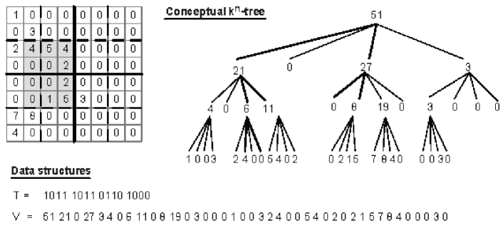
Figure 1: $k^{n}$-treap with a highlighted range query

The navigation through the $k^{n}$-treap is basically a depth first traversal. Finding the child of a node can be done very efficiently by using $rank$ and $select$ operations [9] as in the standard $k^{2}$-tree. The typical queries in this context are: finding the value of an individual cell and finding the sum of the values in a given range of cells, specified by the initial and final coordinates that define the submatrix of interest.

Finding the value of a specific cell by its coordinates.

To find the value of the cell, for example the cell at coordinates $(4,3)$ in the figure, the search starts at the root node and in each step goes down trough the children of the matrix overlapping the searched cell. In this example, the search goes through the first child node (with value 21 in the figure), then through its third child (with value 6) and finally through the second child, reaching the leaf node with value 4, which is the value returned by the query.

Finding the sum of the cells in a submatrix.

The second type of query looks for the aggregated value of a range of cells, like the shaded area in Figure 1. This is implemented as a depth-first multi-branch traversal of the tree. If the algorithm finds that the range specified in the query fully contains a submatrix of the $k^{n}$-treap that has a precomputed sum, it will use this sum and will not descend to its child nodes. The figure highlights the branches of the $k^{n}$-treap that are used. Notice that this query completely includes the sumatrices of values $\{5,4,0,2\}$ and $\{0,2,1,5\}$, that have their sums (11 and 8) explicitly stored on the third level of the tree. Therefore, the algorithm does not need to reach the leaf levels of the tree for these matrices. Notice also that there is an empty submatrix that intersects with the region of the query (the first child of the third child of the root), so the algorithm also stops before reaching the leaf levels in this submatrix. Only for cells $(3,2)$ (with a value of 4) and $(4,2)$ (with a value of 0) needs the algorithm to reach the leaf levels.

3 Our proposal: CMHD

As previously stated, CMHD divides the matrix following the natural hierarchy of the elements in each dimension. In this way we allow the efficient answer of queries that consider the semantic of the dimensions.

3.1 Conceptual description

Consider an $n$-dimensional matrix where each cell contains a weight (e.g., product sales, credit card movements, ad views, etc.). The CMHD recursively divides the matrix into several submatrices, taking into account the limits imposed by the hierarchy levels of each dimension.

Figure 2 depicts an example of a CMHD representation for two dimensions. The matrix records the number of product sales in different locations. For each dimension, a hierarchy of three levels is considered. In particular, cities are aggregated into countries and continents, while products are grouped into sections and good categories. The tree at the right side of the image shows the resulting conceptual CMHD for that matrix. Observe that each hierarchy level leads to an irregular partition of the grid into submatrices (each of them defined by the limits of its elements), having as associated value the sum of product sales of the individual cells inside it. Thus, the root of the tree stores the total amount of sales in the complete matrix. Then the matrix is subdivided by considering the partition corresponding to the first level of the dimension hierarchies (see the bold lines). Each of the submatrices will become a child node of the root, keeping the sum of values of the cells in the corresponding submatrix. The decomposition procedure is repeated for each child, considering subsequent levels of the hierarchies (see the dotted lines), as explained, until reaching the last one. Also notice that, as happens in the $k^{n}$-treap, the decomposition concludes in all branches when empty submatrices are reached (that is, in this scenario, when a submatrix with no sales is found). See, for example, the second child of the root.

Note that CMHD assumes the same height in all the hierarchies that correspond to the different dimensions. Observe that, for each crossing of elements of the same level from different dimensions, an aggregate value is stored. Notice also that artificial levels can be easily added to a hierarchy of one dimension by subdividing all the elements of a level in just one element (itself), thus creating a new level identical to the previous one. This feature allows us to arbitrarily match the levels of the different hierarchies, and thus to flexibly adapt the representation of aggregated data to particular query needs. That is, by introducing artificial intermediate levels where required, more interesting aggregated values will be precomputed and stored. For example, assume we have two dimensions: ($d_{1}$) with levels for department, section and product; and ($d_{2}$) with levels for year, season, month and day. If we were interested in obtaining the number of sales per section for seasons, but also for months, we could devise a new level arrangement for $d_{1}$, that will have now the levels department, section, section’, product; where each particular section of the second hierarchy level results into just one section’ child, which is actually itself. In this way aggregated values will be computed and stored considering sales for section in each season, but also sales for section’ in each month.

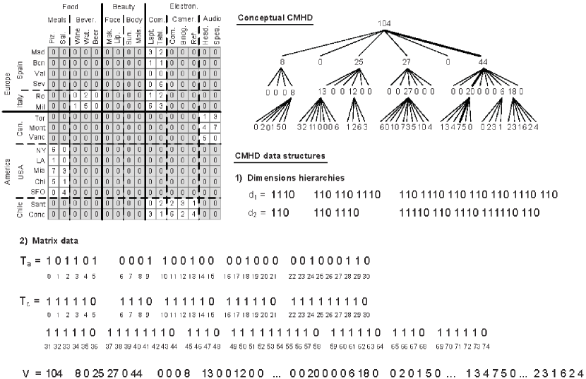
Figure 2: Example of CMHD construction for a two-dimensional matrix.

3.2 Data structures

The conceptual tree that defines the CMHD is represented compactly with different data structures, for the domain hierarchies and for the matrix data itself.

Domain hierarchy representation.

The hierarchy of a dimension domain is essentially a tree of $C$ nodes. We represent this tree using LOUDS [9], a tree representation that uses $2C$ bits, and can efficiently navigate it. Using LOUDS, a tree representing the hierarchy of the elements of a dimension is encoded by appending the degree $r$ of each node in (left-to-right) level-order, in unary: $1^{r}0$. Figure 2 illustrates the hierarchy encoding of the dimensions used in that example (see $d_{1}$ and $d_{2}$). For instance, the degree of the first node for the products dimension ($d_{1}$) is 3, so its unary encoding is 1110. Note that each node (i.e., element of a dimension placed at any level of its hierarchy) is associated with one 1 in the encoded representation of the degree of its parent. LOUDS is navigated using $rank$ and $select$ queries: $rank_{b}(i)$ is the number of bits $b$ up to position $i$, and $select_{b}(j)$ is the position of the $j$th occurrence of bit $b$. Both queries are computed in constant time using $o(C)$ additional bits [6]. For example, given a node whose unary representation starts at position $i$, its parent is $p=select_{0}(t-j)+1$, where $t=select_{1}(j)$ and $j=rank_{0}(i)$; and $i$ is the $(t-p+1)$th child of $p$. On the other hand, the $k$th child of $i$ is $select_{0}(rank_{1}(i)+k-1)+1$. We also use a hash table to associate the domain nodes (i.e., labels such as “USA” in Figure 2) with the corresponding LOUDS node position.

Data representation.

To represent the $n$-dimensional matrix, we use the following data structures:

• Tree structures ($T_{a}$ and $T_{c}$): to navigate the CMHD, we need to use two different data structures in conjunction. First, $T_{a}$, a bit array that, similarly to the $k^{n}$-treap, provides a compact representation of the conceptual tree independently of the node values, for all the tree levels, except the last one. That is, internal nodes whose associated value is greater than 0, will be represented with a 1. In other case, they will be labeled with a 0. Observe that, for the $k^{n}$-treap, the use of this data structure is enough to navigate the tree, taking advantage of the regular partition of the matrix into equal-sized submatrices. Instead, CMHD follows different hierarchy partitions, which results into irregular submatrices. Therefore, a second data structure, $T_{c}$, is also required to traverse the CMHD. This is a bit array aligned to $T_{a}$, which marks the limits of each tree node in $T_{a}$ (this time, it also considers the last tree level). If the next tree node in $T_{a}$ has $z$ children, we append $1^{z-1}0$ to $T_{c}$. Notice that each node of $T_{a}$ is associated with a 0 in $T_{c}$, which allows navigating the trees using $rank$ and $select$ on $T_{a}$ and $T_{c}$: say we are at a node in $T_{a}$ that starts at position $i$; then it has a $k$th child iff $T_{a}[i+k-1]=1$, and if so this child starts at position $select_{0}(T_{c},rank_{1}(T_{a},i+k-1))+1$.

• Values (V): the CMHD is traversed levelwise storing the values associated with each node (either corresponding to original matrix cells, or to data aggregations) in a single sequence, which is then represented with DACs [2].

3.3 Queries

Queries in this context give the names of elements of the different dimensions and ask for the sum of the cells defined for those values. Depending on the query, we can answer it by just reporting a single aggregated value already kept in V, or by retrieving several stored values, and then adding them up. The first scenario arises when the elements (labels) of the different dimensions specified in the query are all at the same level in their respective hierarchies. The second situation arises from queries using labels of different levels. In both contexts, top-down traversals of the conceptual CMHD are required to fetch the values. The algorithm always starts searching the hash tables for the labels provided by the query for the different dimensions, to locate the corresponding LOUDS nodes. From the LOUDS nodes, we traverse each hierarchy upwards to find out its depth and the child that must be followed at each level to reach it.

This information is then used to find the desired nodes in $T_{a}$. For example, with two dimensions, we start at the root of $T_{a}$ and descend to the child number $k_{1}+a_{1}\cdot k_{2}$, where $k_{i}$ is the child that must be followed in the $i$th dimension to reach the queried node, and $a_{i}$ is the number of children of the root in the $i$th dimension ($a_{i}$ is easily computed with the LOUDS tree of its dimension). We continue similarly to the node at level 2, and so on, until we reach one of the query nodes in a dimension, say in the first. Now, to reach the other (deeper) node in the second dimension, we must descend by every child in the first dimension, at every level, until reaching the second queried node. Finally, when we have reached all the nodes, we collect and sum up the corresponding values from $V$. Note that, if all the queried nodes are in the same level, we perform a single traversal in $T_{a}$. Note also that, if we find any zero in a node of $T_{a}$ along this traversal, we immediately prune that branch, as the submatrix contains no data.

Example.

Assume we want to retrieve the total amount of speaker sales in Montreal, in Figure 2. Since both labels belong to the same level in both dimension hierarchies (the last one), we will have to retrieve a single stored value in that level. The path to reach it has been highlighted in the conceptual tree of the image. To perform the navigation we must start at the root of the tree (position 0 in $T_{a}$). In the first level, we need to fetch the sixth child (offset 5), as it corresponds to the submatrix including the element to search, in that level. Hence we access position 5 in $T_{a}$. Since $T_{a}[5]=1$, we must continue descending to the next level. Recall that we have a 1 in $T_{a}$ for each node with children, and that each node is associated with just one 0 in $T_{c}$. So the child starts at position $select_{0}(T_{c},rank_{1}(T_{a},5))+1=select_{0}(T_{c},4)+1=22$ in $T_{a}$. In this level we must access the third child (offset 2), so we check $T_{a}[24]=1$. Again, as we are in an internal node, we know that its children are located at position $select_{0}(T_{c},rank_{1}(T_{a},24))+1=select_{0}(T_{c},9)+1=59$. Finally, we reach the third and last level of the tree, where we know that the corresponding child is the fourth one (at $T_{a}[59+3]=T_{a}[62]$). Recall, however, that this last level is not represented in $T_{a}$. To perform this final step, we directly look into the array $V$: $V[62+1]=V[63]=7$ is the answer.

In case of queries combining labels of different levels, the same procedure would apply, but having to get the values corresponding to all the possible combinations with the element of the lowest hierarchy level (e.g., if we want to obtain the number of meal sales in America, we must first recover the values associated with meal-Canada, meal-USA, and meal-Chile, and then sum them up).

4 Experimental Evaluation

This section presents the empirical evaluation of the two previously described data structures. Both representations have been implemented in C/C++, and the compiler used was GCC 4.6.1. (option -O$9$). We ran our experiments in a dedicated Intel(R) Core(TM) i7-3820 CPU @ 3.60GHz (4 cores) with 10MB of cache, and 64GB of RAM. The machine runs Ubuntu 12.04.5 LTS with kernel 3.2.0-99 (64 bits).

We generate different datasets, all of them synthetic, to evaluate the performance of the two data structures, varying the number of dimensions and the number of items on each dimension. These datasets have been labeled as <dim#>D_<item#>, thus referring to their size specifications in the own name. For example, dataset 5D_16 has 5 dimensions, and the number of items on each dimension is 16. The total size of this dataset is $16^{5}=1048576$ elements.

In order to show the CMHD advantage of considering the domain semantics, and computing the aggregate values according to the natural limits imposed by the hierarchy of elements in each dimension, the dimensions hierarchies have been generated in two different ways for each dataset. First, the binary organization, that corresponds to a regular partition. That is, the hierarchies of each dimension are exactly the same as those produced by a $k^{n}$-treap matrix partition into equal-sized submatrices. In this way both data structures store exactly the same aggregated values. We named it binary because we use a value of $k=2$. Second, the irregular organization, which arbitrary groups data, on each dimension, into different and irregular hierarchies (different number of divisions, and also different size at each level). The last scenario simulates what would be a matrix partition following the semantic needs of a given domain. In this case the aggregated values stored by the CMHD will be different from those stored by the $k^{n}$-treap, and therefore more appropriated to answer queries using the same “semantic”. That means, in our context, queries considering regions that exactly match the natural divisions of each dimension at some level of the hierarchies.

To test the structures behavior, we have also considered three different datasets, with a different number of empty cells, for each size specification: with no empty cells, and with 25% and 50% of empty cells, respectively.

First we analyze the space requirements of both data structures for all the datasets (see Table 1). Of course, the size decreases as the number of empty cells increases, in both cases. Moreover, we can also observe that the $k^{n}$-treap size is slightly lower than the CMHD. This is expected, because CMHD has to store the LOUDS representation of each dimension hierarchy, while dimensions are implicit for the $k^{n}$-treap. Additionally, CMHD uses a second bitmap ($T_{c}$) to navigate the conceptual tree, which is not necessary when using the $k^{n}$-treap.

We must also clarify a small issue about the sizes of the $k^{n}$-treaps: the size of a standard $k^{n}$-treap for a specific dataset is always the same, regardless of the organization of its dimensions (binary or irregular). However, Table 1 shows some difference in the sizes. For example, for 4D_16, the size for the binary organization is $44.84$, but it is $44.42$ for the irregular one. The reason for this variation is that all queries are performed by taking dimension labels as input, so we need a vocabulary to translate each label into a range of cells. We have included that vocabulary (dimension labels and cell ranges) into the size of the $k^{n}$-treaps, and the vocabulary for the irregular organization is usually smaller, as it has less levels and less dimension labels (because each node in the conceptual tree can have more than 2 children in the irregular organization, while the binary organization always has 2).

	0% Zeroes				25% Zeroes				50% Zeroes
	Binary		Irregular		Binary		Irregular		Binary		Irregular
name	kn-treap	CMHD	kn-treap	CMHD	kn-treap	CMHD	kn-treap	CMHD	kn-treap	CMHD	kn-treap	CMHD
4D_16	44.84	55.56	44.22	47.82	38.16	47.54	37.54	43.04	29.51	37.09	28.89	34.18
4D_32	680.45	864.17	679.08	750.17	552.15	710.05	550.78	640.80	400.13	527.57	398.76	501.01
5D_16	631.10	793.34	630.41	729.48	527.23	667.69	526.54	653.25	408.10	523.27	407.41	509.80
5D_32	20098.99	25328.26	20097.43	23344.18	16272.61	20691.87	16271.04	20167.62	11776.94	15237.57	11775.37	15471.61
6D_16	9663.37	12073.82	9662.48	11456.36	8180.31	10278.04	8179.43	10532.61	6419.99	8135.86	6419.11	8279.60

Table 1: Space requirements of $k^{n}$-treap and CMHD data structures (in KB)

Regarding query times, we have run several sets of queries for all the datasets. As previously mentioned, queries are posed in this context by giving one element name (label) for each different dimension, as it is the natural way to query a multidimensional matrix defined by hierarchical dimensions. Since the $k^{n}$-treap does not directly work with labels, each query has been translated into the equivalent ranged query, establishing the initial and final coordinates for each dimension. The following types of queries have been considered:

• Finding one precomputed value. This value can be a specific cell of the matrix (so forcing the algorithms to reach the last level of the tree), or a precomputed value that corresponds to an internal node of the conceptual tree.

  Following the example of Figure 2, a query asking for the amount of speakers sales in Montreal or the total number of beberages sales in Italy would be queries of this type, the former accessing an individual cell and the later obtaining a precomputed value in the penultimate level of the tree.

• Finding the sum of several precomputed values. This kind of query must obtain a sum that is not precomputed and stored in the data structure itself. In turn, it must access several of these aggregated values and then add them up. Given that we are specifying the queries by dimension labels, this type of query is defined by using labels that belong to different levels of the hierarchies across the dimensions. The lowest level, which corresponds to individual cells, is not used for this scenario.

  An example of this query type would be to find the total number of sales of electronic products in Chile. Note that electronic is located at the first level of its dimension hierarchy, but Chile is at the second level of the second dimension (see Figure 2). Hence, the values corresponding to computers-Chile, cameras-Chile, and audio-Chile must be first retrieved to finally sum them up.

Each created set contains $10,000$ queries, randomly generated, of the two previous types, for each dataset. The following tables show the average query times (in microseconds per query) for both data structures, taking into account the two different matrix partitions of the datasets (binary or irregular) and also the percentage of empty cells.

We first show the results obtained for queries that just need to retrieve one precomputed value, at different levels. On the one hand, Table 2 displays query times for specific matrix cells, that is, located at the last level of the conceptual tree. In this case, the $k^{n}$-treap performs better than the CMHD in almost all cases. This is an expected outcome as both data structures must reach the leaf level to get the answer, and the depth first navigation of the tree is simpler in the $k^{n}$-treap (just products and $rank$ operations). In any case, CMHD also performs quite well, using just a few microseconds to answer any of the queries.

	0% Zeroes				25% Zeroes				50% Zeroes
	Binary		Irregular		Binary		Irregular		Binary		Irregular
Dataset	kn-treap	CMHD	kn-treap	CMHD	kn-treap	CMHD	kn-treap	CMHD	kn-treap	CMHD	kn-treap	CMHD
4D_16	2	4	2	3	2	4	2	2	2	4	2	3
4D_32	2	5	3	4	2	4	2	1	2	4	1	4
5D_16	2	4	3	4	2	5	3	2	2	5	2	2
5D_32	3	6	3	5	2	4	3	3	2	6	3	2
6D_16	3	4	3	4	3	6	4	2	4	5	4	4

Table 2: Average query times (in $\mu$s) for queries finding one precomputed value (original matrix cells).

On the other hand, Table 3 shows the average query times for queries of the same type, but now considering precomputed values stored in nodes of an intermediate level of the tree (in particular, the penultimate level). Note that this fact holds for both data structures when working with a regular partition of the matrix (that is, the binary scenario). Thus, in this case, the $k^{n}$-treap gets better results than CMHD, but with slight time differences. Yet, observe that this is not the actual scenario when dealing with meaningful application domains, where rich semantics arise. This situation is that corresponding to what we called irregular datasets. In this case, CMHD excels, as expected, given that this data structure has been particularly designed to manage hierarchical domains. Results show that CMHD is able to perform up to 12 times faster than $k^{n}$-treap (for the best case).

	0% Zeroes				25% Zeroes				50% Zeroes
	Binary		Irregular		Binary		Irregular		Binary		Irregular
Dataset	kn-treap	CMHD	kn-treap	CMHD	kn-treap	CMHD	kn-treap	CMHD	kn-treap	CMHD	kn-treap	CMHD
4D_16	1	4	7	3	1	3	6	2	2	4	5	2
4D_32	1	3	9	3	1	3	7	2	1	3	6	1
5D_16	2	4	11	1	2	3	9	1	2	4	7	3
5D_32	3	4	23	2	2	4	18	3	2	3	12	2
6D_16	2	4	35	2	2	2	28	3	3	4	21	1

Table 3: Average query times (in $\mu$s) for queries finding one precomputed value (penultimate tree level).

To check whether the observed differences are significative (in the cases where times were closer) we performed a statistical significance test. We checked the 4D_16 and 5D_16 datasets, for the irregular organization, with all the different configurations of empty cells.

We show here, as a proof, the details for 4D_16 with 50% of empty cells, which took $5\mu\mbox{s}$ to the $k^{n}$-treap, and $2\mu\mbox{s}$ to CMHD. We ran 20 sets of $10,000$ queries, and measured both the average time and the standard deviation for the $k^{n}$-treap ($5.100$ and $0.447$, respectively) and for the CMHD ($1.750$ and $0.550$, respectively). With these results, we obtain a critical value of $4.725$, which is greater than $2.580$, so the difference is significative with a 99% of confidence level. The remaining tests also proved the same significance results.

Finally, Table 4 presents the average query times for the second type of queries (that is, those having to recover several precomputed values and then adding them up to provide the final answer). As results show, the $k^{n}$-treap displays a better performance than CMHD for the binary scenario. However, again this is not the most interesting situation in real domains. If we observe the results obtained for the irregular datasets, we will appreciate that CMHD clearly outperforms the $k^{n}$-treap in this scenario, thus demonstrating the good capabilities of our proposal to cope with the aim of this work.

	0% Zeroes				25% Zeroes				50% Zeroes
	Binary		Irregular		Binary		Irregular		Binary		Irregular
Dataset	kn-treap	CMHD	kn-treap	CMHD	kn-treap	CMHD	kn-treap	CMHD	kn-treap	CMHD	kn-treap	CMHD
4D_16	3	10	20	4	3	6	16	3	2	6	12	6
4D_32	6	21	21	3	4	20	17	4	4	20	12	5
5D_16	4	8	30	8	4	8	25	3	3	7	19	1
5D_32	6	26	49	3	8	23	39	5	6	21	27	2
6D_16	5	15	106	7	5	10	82	6	4	9	63	8

Table 4: Average query times (in $\mu$s) for queries finding a sum of precomputed values.

5 Conclusions and Future Work

We have presented a multidimensional compact data structure that is tailored to perform aggregate queries on data cubes over hierarchical domains, rather than general range queries. The structure represents each hierarchy with a succinct tree representation, and then partitions the data cube according to the product of the hierarchies. This partition is represented with an extension of the $k^{2}$-treap to higher dimensions and to non-regular partitions. The resulting structure, dubbed CMHD, is much faster than a regular multidimensional $k^{2}$-treap when the queries follow the hierarchical domains. This makes it particularly attractive to represent OLAP data cubes compactly and efficiently answer meaningful aggregate queries.

As future work, we plan to experiment on much larger collections. This would make the vocabulary of hierarchy nodes much less significant compared to the data itself (especially for the CMHD). We also plan to test real datasets (for example, coming from data warehouses) and real query workloads. We also expect to compare our results with established OLAP database management systems, and to enrich our prototype with other kinds of queries and data.

References

- [1] Brisaboa, N.R., de Bernardo, G., Konow, R., Navarro, G., Seco, D.: Aggregated 2d range queries on clustered points. Information Systems pp. 34–49 (2016)
- [2] Brisaboa, N.R., Ladra, S., Navarro, G.: Dacs: Bringing direct access to variable-length codes. Information Processing and Management pp. 392–404 (2013)
- [3] Brisaboa, N.R., Ladra, S., Navarro, G.: Compact representation of web graphs with extended functionality. Information Systems pp. 152–174 (2014)
- [4] Chan, T., Durocher, S., Larsen, K., Morrison, J., Wilkinson, B.: Linear-space data structures for range mode query in arrays. In: Proc. 29th International Symposium on Theoretical Aspects of Computer Science (STACS). pp. 290–301 (2012)
- [5] Chaudhuri, S., Dayal, U.: An Overview of Data Warehousing and OLAP Technology. SIGMOD Rec. 26(1), 65–74 (Mar 1997)
- [6] Clark, D.: Compact PAT Trees. Ph.D. thesis, University of Waterloo, Canada (1996)
- [7] Codd, E.F., Codd, S.B., Salley, C.T.: Providing OLAP (On-Line Analytical Processing) to User-Analysts: An IT Mandate. E. F. Codd and Associates (1993)
- [8] Hon, W., Shah, R., Thankachan, S.V., Vitter, J.S.: Space-efficient frameworks for top-k string retrieval. Journal of the ACM 61(2), 9:1–9:36 (2014)
- [9] Jacobson, G.: Space-efficient static trees and graphs. In: Proceedings of the 30th Annual Symposium on Foundations of Computer Science. pp. 549–554. SFCS ’89, IEEE Computer Society, Washington, DC, USA (1989)
- [10] Kimball, R., Ross, M.: The Data Warehouse Toolkit: The Complete Guide to Dimensional Modeling. John Wiley & Sons, Inc., New York, NY, USA, 2nd edn. (2002)
- [11] Larsen, K., van Walderveen, F.: Near-optimal range reporting structures for categorical data. In: Proc. 24th Symposium on Discrete Algorithms (SODA). pp. 265–276 (2013)
- [12] Levene, M., Loizou, G.: Why is the snowflake schema a good data warehouse design? Information Systems 28(3), 225–240 (2003)
- [13] Sadakane, K.: Succinct data structures for flexible text retrieval systems. Journal of Discrete Algorithms 5, 12–22 (2007)
- [14] Samet, H.: Foundations of Multidimensional and Metric Data Structures. Morgan Kaufmann (2006)