Modified Cholesky Riemann Manifold Hamiltonian Monte Carlo: Exploiting Sparsity for Fast Sampling of High-dimensional Targets

Abstract

Riemann manifold Hamiltonian Monte Carlo (RMHMC) has the potential to produce high-quality Markov chain Monte Carlo-output even for very challenging target distributions. To this end, a symmetric positive definite scaling matrix for RMHMC, which derives, via a modified Cholesky factorization, from the potentially indefinite negative Hessian of the target log-density is proposed. The methodology is able to exploit the sparsity of the Hessian, stemming from conditional independence modelling assumptions, and thus admit fast implementation of RMHMC even for high-dimensional target distributions. Moreover, the methodology can exploit log-concave conditional target densities, often encountered in Bayesian hierarchical models, for faster sampling and more straight forward tuning. The proposed methodology is compared to alternatives for some challenging targets, and is illustrated by applying a state space model to real data.

Keywords: Bayesian hierarchical models, Hamiltonian Monte Carlo, Hessian, MCMC, metric tensor

1 Introduction

Markov chain Monte Carlo (MCMC) methods have by now seen widespread use for sampling from otherwise intractable distributions in statistics for close to three decades (Gelman et al., 2014). Still the development of new and improved MCMC methods for tackling ever more challenging sampling problems is a highly active field (see e.g. Andrieu et al., 2010; Girolami and Calderhead, 2011; Calderhead, 2014; Hoffman and Gelman, 2014). The contribution of the present work is a new metric tensor, deriving directly from the Hessian of the log-target density that, together with Riemann manifold Hamiltonian Monte Carlo (RMHMC) (Girolami and Calderhead, 2011) enables fast and robust sampling from target distributions with strong non-linear dependencies. Such target distributions arise, for instance, as the joint posterior distribution of latent variables and parameters in non-linear and/or non-Gaussian Bayesian hierarchical models.

Current MCMC strategies for Bayesian inference in such hierarchical models can informally be split into three categories (see also Betancourt and Girolami, 2013, for a similar discussion): 1) Variants of Gibbs sampling, 2) Pseudo-marginal methods and 3) methods that update latent variables and parameters jointly. Gibbs sampling (see e.g. Liu, 2001; Robert and Casella, 2004) is widely used as it is, in many cases, relatively easy to implement. However, it is well known that naive Gibbs sampling for hierarchical models, where e.g. the latent variables are in one block and the variance parameter of the latent variables is in another block, can lead to poor mixing due to strong non-linear dependencies across the blocks.

Pseudo-marginal methods (see e.g. Andrieu et al., 2010; Pitt et al., 2012) on the other hand, seek to avoid such poor mixing by targeting directly the marginal posterior of the parameters (i.e. with the latent variables integrated out). However, such methods hinge on the ability to Monte Carlo simulate an unbiased, low variance estimate of marginal posterior density of the parameters, which can often be extremely computationally demanding (Flury and Shephard, 2011), or even infeasible for larger models.

Finally, methods that update the latent variables and parameters jointly are attractive in theory as they also avoid the non-linear dependency problems of Gibbs sampling, and they do not need computationally demanding marginal density estimates. However, such methods need mechanisms for aligning the proposals with the local geometry of the target, in particular for high-dimensional problems. Currently, popular methods within this category are Metropolis-adjusted Langevin methods (see e.g. Roberts and Stramer, 2002; Girolami and Calderhead, 2011; Xifara et al., 2014; Kleppe, 2016) and various variants of Hamiltonian Monte Carlo (see e.g. Duane et al., 1987; Neal, 1996, 2010; Girolami and Calderhead, 2011; Betancourt, 2013a; Lan et al., 2015). Both use derivative information from the target log-density to guide the MCMC proposals. However, it has become clear (see e.g. Betancourt, 2013a) that methods based on first order derivatives only (as is done in the default MCMC method in the popular Bayesian computation software Stan (Carpenter et al., 2017)), can be inefficient if one fails to take the local scaling properties of the target into account. This mirrors the relation between the method of steepest descent and Newton’s method in numerical optimisation (Nocedal and Wright, 1999).

Joint updating of latent variables and parameters in Bayesian hierarchical models is also the main motivation of this paper, even though the methodology is applicable for any continuous target distribution under some regularity conditions. Here a particular modified Cholesky factorization is proposed, that when applied to a potentially indefinite negative Hessian of the log-target, produces useful scaling information for RMHMC. In conjunction, RMHMC and the proposed methodology enables MCMC sampling where the proposals are far from the current configuration, and that is robust to significantly different scaling properties across the support of the target, a property often seen in Bayesian hierarchical models. It is worth noticing that applying modified negative Hessians in RMHMC (Betancourt, 2013a) or when scaling MCMC proposals in general (Geweke and Tanizaki, 1999, 2003; Qi and Minka, 2002; Martin et al., 2012; Kleppe, 2016) is not new per se. However, the proposed modified Cholesky approach is, by exploiting sparsity of the negative Hessian, computationally fast and scalable in the dimension of the target.

The exploitation of sparsity is increasingly important in the numerical linear algebra involved in modern statistical computing associated with hierarchical models, as the dimension of matrices to be factorized can easily reach $\sim 10^{5}$ (see e.g. Rue, 2001; Rue and Held, 2005; Rue et al., 2009). The sparsity of involved Hessian matrices arises due to conditional independence assumptions used in the modelling. Examples include block-diagonal structures associated with non-linear mixed effect regressions, banded structures for Markovian dynamic models with unobserved factors such as state space models, and less structured sparse matrices for spatial/spatial-temporal models that involve Gaussian Markov random fields (see e.g. Lindgren et al., 2011). Currently, the Integrated Nested Laplace Approximation (INLA) (Rue et al., 2009) is a widely used methodology for fast approximate Bayesian inference in the Latent Gaussian Model (LGM) sub-class of Bayesian hierarchical models. Like the proposed methodology, INLA relies heavily on exploiting sparsity in order to speed up computations, and in the context of LGMs, the proposed methodology can also benefit from the fact that conditional posterior log-densities of the latents are concave. However, the proposed methodology is more general with respect to models that can be handled, and in particular does not require the LGM-assumption that the latent variables have a joint Gaussian prior (see Section 5), or the INLA-assumption that the number of parameters is small.

The remainder of the paper is laid out as follows: Section 2 fixes notation and reviews RMHMC. Section 3 describes and discusses the proposed methodology. In Section 4, the proposed methodology is compared to Gibbs sampling, Euclidian metric Hamiltonian Monte Carlo (EHMC), The no-u-turn sampler (NUTS) of Stan and RMHMC based on spectral decompositions for two challenging target distributions. Section 5 describes an application to a non-linear, non-Gaussian state space model, and finally Section 6 provides some discussion.

2 Riemann manifold HMC

This section fixes notation and reviews RMHMC (Girolami and Calderhead, 2011) in order to set the stage. Denote by $\nabla_{\mathbf{y}}$ the gradient/Jacobian operator with respect to vector $\mathbf{y}$, $|A|$ the determinant of square matrix $A$, and $I_{d}$ denotes the $d$-dimensional identity matrix. A natural matrix norm is denoted by $\|\cdot\|$ and $\Phi$ is the standard normal cumulative distribution function.

Let $\tilde{\pi}(\mathbf{x})$ denote a density kernel associated with the target density $\pi(\mathbf{x}):\Omega\rightarrow\mathbb{R}^{+}$ where $\Omega\subseteq\mathbb{R}^{d}$. It is assumed that $\tilde{\pi}(\mathbf{x})$ is continuous and has continuous derivatives up to order 3. Moreover, let the metric tensor $G(\mathbf{x})$ be a symmetric positive definite $d\times d$ matrix for all $\mathbf{x}\in\Omega$, where $G_{i,j}(\mathbf{x}):\Omega\rightarrow\mathbb{R}$ are smooth functions for all $i,j=1,\dots,d$. Particular choices of $G(\mathbf{x})$ will be discussed in detail in Section 3.

Like for other Hamiltonian Monte Carlo methods, RMHMC relies on defining a synthetic Hamiltonian dynamical system that evolves over fictitious time $\tau$, where $\mathbf{x}$ plays the role of position variable and $\mathbf{p}\in\mathbb{R}^{d}$ is the (auxiliary) momentum variable. The total energy in the system is given by the Hamiltonian $H(\mathbf{x},\mathbf{p})$, which for RMHMC is taken to be

$$H(\mathbf{x},\mathbf{p})=-\log\tilde{\pi}(\mathbf{x})+\frac{1}{2}\log(|G(\mathbf{x})|)+\frac{1}{2}\mathbf{p}^{T}G(\mathbf{x})^{-1}\mathbf{p}.$$ (1)

The time-evolution of $(\mathbf{x}(\tau),\mathbf{p}(\tau))$ is described by Hamilton’s equations

$$\frac{\partial}{\partial\tau}\mathbf{x}(\tau) = \nabla_{\mathbf{p}}H(\mathbf{x}(\tau),\mathbf{p}(\tau))=G(\mathbf{x}(\tau))^{-1}\mathbf{p(\tau)},$$ (2)

$$\frac{\partial}{\partial\tau}\mathbf{p}(\tau) = -\nabla_{\mathbf{x}}H(\mathbf{x}(\tau),\mathbf{p}(\tau)).$$ (3)

Let $\mathbf{z}(\tau)=(\mathbf{x}(\tau)^{T},\mathbf{p}(\tau)^{T})^{T}\in\mathbb{R}^{2d}$ be the state of the system at time $\tau$ and likewise define $H(\mathbf{z}(\tau))=H(\mathbf{x}(\tau),\mathbf{p}(\tau))$. Moreover, let $\varphi_{\tau}(\cdot):\mathbb{R}\times\Omega\rightarrow\Omega$ denote the flow of $\mathbf{z}$ associated with (2,3) so that $\mathbf{z}(r+s)=\varphi_{s}(\mathbf{z}(r))\;\forall r,s\in\mathbb{R}$ whenever $\mathbf{z}(\tau)$ solves (2,3). The following properties of the Hamiltonian flow $\varphi_{\tau}$ can be established (see e.g. Leimkuhler and Reich, 2004)

• Energy conservation, i.e. $H(\varphi_{\tau}(\mathbf{z}))$ is constant as a function of $\tau$ for any $\mathbf{z}\in\Omega$.

• Time-reversibility, i.e. the inverse of $\varphi_{\tau}$ is $\varphi_{-\tau}$ so that $\varphi_{-\tau}(\varphi_{\tau}(\mathbf{z}))=\mathbf{z}$ for any $\mathbf{z}\in\Omega$.

• $\varphi_{\tau}$ is said to be symplectic, namely for each $\tau$, $(\nabla_{\mathbf{z}}\varphi_{\tau}(\mathbf{z}))^{T}J(\nabla_{\mathbf{z}}\varphi_{\tau}(\mathbf{z}))=J$ where

  $$J=\left[\begin{array}[]{cc}0&I_{d}\\ -I_{d}&0\end{array}\right].$$

  In particular, the symplecticity implies that $\varphi_{\tau}$ is a volume-preserving map so that the Jacobian $\nabla_{\mathbf{z}}\varphi_{\tau}(\mathbf{z})$ has unit determinant.

Based on these properties, it is relatively straight forward to verify that $\varphi_{\tau}$ preserves the Bolzmann distribution

$$\pi(\mathbf{z})=\pi(\mathbf{x},\mathbf{p})\propto\exp(-H(\mathbf{x},\mathbf{p})).$$

Namely, provided that $\mathbf{z}\sim\pi(\mathbf{z})$, then also $\varphi_{\tau}(\mathbf{z})\sim\pi(\mathbf{z})$ for any $\tau\in\mathbb{R}$. Given the particular specification of the Hamiltonian (1), the Bolzmann distribution admits the target distribution $\pi(\mathbf{x})$ as the $\mathbf{x}$-marginal. To see this, observe that

$$\int\pi(\mathbf{x},\mathbf{p})d\mathbf{p}\\ \propto\hat{\pi}(\mathbf{x})|G(\mathbf{x})|^{-\frac{1}{2}}\int\exp\left(-\frac{1}{2}\mathbf{p}^{T}G(\mathbf{x})^{-1}\mathbf{p}\right)d\mathbf{p}\\ \propto\hat{\pi}(\mathbf{x}).$$ (4)

Granted the above constructions, an ideal MCMC algorithm for obtaining (dependent) samples $\{(\mathbf{x}_{t},\mathbf{p}_{t})\}_{t}\sim\pi(\mathbf{x},\mathbf{p})$ would be to alternate between 1) sample $\mathbf{p}_{t-1}\sim\pi(\mathbf{p}|\mathbf{x}_{t-1})=N(0,G(\mathbf{x}_{t-1}))$, and 2) compute $(\mathbf{x}_{t},\mathbf{p}^{*})=\varphi_{\tau}((\mathbf{x}_{t-1},\mathbf{p}_{t-1}))$ for some $\tau$. However, for most non-trivial target distributions and metric tensors, such an algorithm is infeasible as the corresponding $\varphi_{\tau}$s do not admit closed form expressions. Instead, RMHMC relies on approximate numerical simulation of the flow and correcting for the numerical error using an accept-reject step.

2.1 Numerical simulation of the flow and RMHMC

In order to simulate the flow numerically, the splitting method integrator of Betancourt (2013a) was used. This integrator preserves the time-reversibility and symplectic nature of the flow, while only approximately preserves the total energy. Though alternative, potentially less computationally intensive, non-symplectic implementations exist (see e.g. Lan et al., 2015), a symplectic integrator was chosen, as it admits stable and accurate numerical simulation of the flow for large $d$ and potentially long time spans. Moreover, using a symplectic and time-reversible integrator leads to simple expressions for the accept probability used in the accept/reject step.

The integrator of Betancourt (2013a) for approximating $\varphi_{\varepsilon}(\mathbf{z}(\tau))$, for some small time step $\varepsilon$, is characterized by

$$\hat{\mathbf{p}}_{*}=\mathbf{p}(\tau)\\ -\frac{\varepsilon}{2}\nabla_{\mathbf{x}}\left[-\log\tilde{\pi}(\mathbf{x}(\tau))+\frac{1}{2}\log(|G(\mathbf{x}(\tau))|)\right],$$ (5)

$$\hat{\mathbf{p}}_{**}=\hat{\mathbf{p}}_{*}-\frac{\varepsilon}{2}\nabla_{\mathbf{x}}\left[\frac{1}{2}\mathbf{\hat{p}_{**}}^{T}G(\mathbf{x}(\tau))^{-1}\hat{\mathbf{p}}_{**}\right],$$ (6)

$$\hat{\mathbf{x}}(\tau+\varepsilon)=\mathbf{x}(\tau)+\frac{\varepsilon}{2}G^{-1}(\mathbf{x}(\tau))\hat{\mathbf{p}}_{**}\\ +\frac{\varepsilon}{2}G^{-1}(\hat{\mathbf{x}}(\tau+\varepsilon))\hat{\mathbf{p}}_{**},$$ (7)

$$\hat{\mathbf{p}}(\tau+\varepsilon)=\hat{\mathbf{p}}_{**}-\frac{\varepsilon}{2}\nabla_{\mathbf{x}}H(\mathbf{x}(\tau+\varepsilon),\hat{\mathbf{p}}_{**}),$$ (8)

where $\hat{\mathbf{x}}(\tau)$ and $\hat{\mathbf{p}}(\tau)$ denote the approximations to $\mathbf{x}(\tau)$ and $\mathbf{p}(\tau)$ respectively. Applying the integrator (5-8) sequentially $l=1,2,\dots$ times produces approximations to the flow after $\varepsilon l$ time has passed. A single transition $\mathbf{x}_{t-1}\rightarrow\mathbf{x}_{t}$ of the basic RMHMC algorithm used throughout this paper can be summarized by the steps:

1. Resample momentums $\mathbf{p}_{t-1}\sim\pi(\mathbf{p}|\mathbf{x}_{t-1})=N(0,G(\mathbf{x}_{t-1}))$.

2. Sample $l$ and $\varepsilon$, and perform $l$ integrator steps with step size $\varepsilon$ starting at $(\text{$\mathbf{x}$}_{t-1},\mathbf{p}_{t-1})$. This process results in the proposal $(\mathbf{x}_{t}^{*},\mathbf{p}_{t}^{*})$.

3. With probability $\min(1,\exp(-H(\mathbf{x}_{t}^{*},\mathbf{p}_{t}^{*})+H(\text{$\mathbf{x}$}_{t-1},\mathbf{p}_{t-1})))$ set $\mathbf{x}_{t}=\mathbf{x}_{t}^{*}$, and with remaining probability set $\mathbf{x}_{t}=\mathbf{x}_{t-1}$.

Other, more complicated and potentially more efficient variants of the overarching RMHMC algorithm, such as algorithms choosing the number of integration steps dynamically (Betancourt, 2013b, 2016) are also conceivable in this framework. Such dynamic selection is likely to be required in more automated implementations of the proposed methodology. However, the basic RMHMC method outlined above was used, as the focus of the present paper is on the particular metric tensor advocated.

It is worth noticing that (6,7) are implicit and therefore necessitate computationally costly fixed point iterations (Leimkuhler and Reich, 2004). In fact, the bulk part of the computation is spent computing the derivatives of $H$ needed for solving (6,7), and therefore implementing the solution process in an efficient manner is of high importance. In the present implementation, the fixed point iterations are continued until the infinity-norm of the difference between successive iterates is $<1.0e-6$. To meet this tolerance in the real application with $d=3087$ considered in Section 5, 5-6 iterations are required in (6) and 3-4 iterations are required in (7).

3 Metric tensor based on a modified Cholesky factorization

This section describes the proposed metric tensor, and thereby the implied Riemann manifold intended for RMHMC and related methods. By now, a rich literature considering the differential geometric properties of RMHMC has appeared (see e.g. Betancourt et al., 2016). In this paper, a slightly less mathematically inclined approach is taken, and rather focus lies on some intuition and how to implement RMHMC for a general target distribution.

3.1 Metric tensor from the negative Hessian

For EHMC, a rule of thumb is that a constant $G$ should be taken as the precision matrix of the target for near-Gaussian targets (Neal, 2010). For RMHMC, several papers have argued for a metric tensor deriving from (negative) second derivative information, specifically the Fisher information matrix (Girolami and Calderhead, 2011; Lan et al., 2015) or a regularized version of the negative log-target density Hessian (see e.g. Sanz-Serna, 2011; Guerrera et al., 2011; Jasra and Singh, 2011). Modulus regularisation, the latter fulfils the rule of thumb for EHMC and Gaussian targets. For a model where the Fisher information matrix is available, it is likely that the information matrix approach is preferable, as the information matrix is by construction positive definite. However, for a general model, the information matrix is either not available in closed form or requires substantial analytic calculations for each model instance. In the reminder of the paper, unavailable Fisher information matrix is taken as a premise for the discussion.

In deriving the metric tensor directly from the negative Hessian, computing expectations is no longer needed, but on the other hand, accounting for the fact that the negative Hessian often is indefinite in non-negligible subsets of $\Omega$ is required. Betancourt (2013a) introduced the softmax metric, which is based on a full spectral decomposition of the negative Hessian and a subsequent regularisation of the eigenvalues. This method is attractive as it retains the eigenvectors of the negative Hessian, but is very computationally demanding for large models. The present work is similar to Betancourt (2013a) in deriving $G$ directly from the Hessian, but the computational details are different.

An additional rationale for choosing $G$ to be a regularized approximation to the negative Hessian is as follows. It is relatively straight forward to verify that a RMHMC proposal for $\mathbf{x}$ using a single time integration step (using the generalized leapfrog integrator (Girolami and Calderhead, 2011; Leimkuhler and Reich, 2004, page 156)), starting at $\mathbf{x}(0)$ will have the mean

$$E(\hat{\mathbf{x}}(\varepsilon)|\mathbf{x}(0))=\mathbf{x}(0)\\ +\frac{\varepsilon^{2}}{2}\left[G^{-1}(\mathbf{x}(0))\left[\nabla_{\mathbf{x}}\log\tilde{\pi}(\mathbf{x}(0))\right]+\Lambda(\mathbf{x}(0))\right]\\ +O(\varepsilon^{4}),$$ (9)

where

$$\Lambda_{i}(\mathbf{x})=\sum_{j=1}^{d}\frac{\partial}{\partial x_{j}}G_{i,j}^{-1}(\mathbf{x}),\;i=1,\dots,d.$$

It is seen that the $O(\varepsilon^{2})$ term scales the gradient of the log-target with the inverse of $G$. Therefore choosing $G$ as a regularized version of the negative Hessian will turn the former part of the $O(\varepsilon^{2})$ term into a modified Newton (numerical optimization) direction, which is known to be a well-scaled search direction in the numerical optimization literature (Nocedal and Wright, 1999, Chapter 6). In fact, modulus the effect of the additional term $\Lambda$, choosing $G$ in this manner makes time $\tau$ and the time step $\varepsilon$ effectively dimensionless (Girolami and Calderhead, 2011, Page 132) as there is a unit “natural” step length (Nocedal and Wright, 1999, Page 23) associated with a Newton step. In the present setup, this corresponds to $\tau=O(\sqrt{2})$ is the time needed to traverse to the mode from any region close to a mode.

It is also worth noticing that the additional term $\Lambda$ in (9) is a correction term that accounts for the non-constant curvature of the implied manifold, while retaining the correct Boltzmann distribution associated with (1). In particular, the explicit terms of (9), along with the leading term of

$$Var(\hat{\mathbf{x}}(\varepsilon)|\mathbf{x}(0))=\varepsilon^{2}G^{-1}(\mathbf{x}(0))+O(\varepsilon^{4}),$$

are identical to the first two moments of the proposal associated with the time discretised position dependent metric Langevin diffusion (with $\pi(\mathbf{x})$ as stationary distribution due to the $\Lambda$ term in the drift) of Xifara et al. (2014, Equation 9). This observation mirrors the well-known fact that one (Euclidian metric) Metropolis-adjusted Langevin algorithm proposal is identical to the proposal of one EHMC time integration step, but in the general Riemann manifold case, this correspondence is only asymptotical as $\varepsilon\rightarrow 0$.

At this point, it is also worth contrasting a variable $G(\mathbf{x})$ to a constant $G$, resulting in EHMC. The latter is currently used (either identity, diagonal, or dense matrix) in tandem with the NUTS (Hoffman and Gelman, 2014) as the default sampling algorithm in the widely applied Bayesian computation software Stan (Carpenter et al., 2017). In the constant $G$-case, $\Lambda$ and the higher order terms of (9) vanish, and thus the proposal means are $E(\hat{\mathbf{x}}(\varepsilon)|\mathbf{x}(0))=\mathbf{x}(0)+\frac{\varepsilon^{2}}{2}G^{-1}\left[\nabla_{\mathbf{x}}\log\tilde{\pi}(\mathbf{x}(0))\right]$. For targets with close to constant curvature (i.e. in practice close to Gaussian, often seen for posteriors in non-hierarchical models), this works well, and is substantially faster than the proposed methodology as explicit integrators may be employed. However, for targets exhibiting substantial variation in the curvature, such fixed scaling of the gradient may, for non-negligible subsets of $\Omega$, produce either: 1) too aggressive proposals, leading to inaccurate simulation of the flow and subsequent rejections of the proposals. In turn, this leads in practice to that subsets of $\Omega$ are left unexplored (Betancourt, 2013a). 2) too defensive proposals, leading to slow exploration of subsets of $\Omega$, and in particular may often lead to too small $l$s being selected by NUTS-like algorithms (Betancourt, 2013b). In section 4, it is shown that Stan and EHMC may exhibit such pathologies when MCMC samples are compared to known marginals of the target. However, in practice it is difficult to determine whether such pathologies are active in a given MCMC simulation.

The remainder of this section is devoted to the particular form of metric tensor advocated here.

3.2 A smooth modified Cholesky factorization

This section develops a metric tensor in the form of a regularized approximation of the negative Hessian matrix, which is guaranteed to be positive definite. The approach is similar to the modified Cholesky factorization approach for modified Newton optimization algorithms of Gill and Murray (1974); Gill et al. (1981). The differences amount primarily to making sure that each element of $G$ is a smooth function of $\mathbf{x}$ so that the implied manifold is also smooth. Through a large number of numerical optimization applications, the modified Cholesky approach has proven to be a trusted and frequently used technology (Nocedal and Wright, 1999), and the approximation has also served as the basis for further refinements (Schnabel and Eskow, 1990, 1999). A further motivation for working with modified Cholesky factorizations, as opposed to say methods based on full spectral decompositions, is that this method can be implemented while exploiting sparsity patterns (Davis, 2006) of the negative Hessian often found in statistical models (see e.g. Rue, 2001; Rue et al., 2009).

Denote by $A$ a symmetric matrix (e.g. the negative Hessian) for which a positive definite approximation is sought. The approach for finding $G$ takes as vantage point a square root free Cholesky factorization which produces the (LDL-)decomposition

$$\bar{L}\bar{D}\bar{L}^{T}=A.$$

Here, $\bar{L}$ is unit lower triangular (i.e. 1s on the diagonal) and $\bar{D}$ is a diagonal matrix (Golub and van Loan, 1996, section 4). When $A$ is positive definite, the diagonal elements of $\bar{D}$ are positive, whereas in the indefinite case, the factorization may not exist or it may be numerically unstable and produce arbitrary large elements in $\bar{L}$ and $\bar{D}$ (Nocedal and Wright, 1999, section 6.3). The insight of Gill and Murray (1974); Gill et al. (1981) was that $\bar{D}_{j,j}$ (and consequently the resulting $\bar{L}$) can be modified online to produce a square root free Cholesky factorization $\tilde{L}D\tilde{L}=A+J$ of the symmetric positive definite matrix $A+J$, where $J$ is a diagonal matrix with non-negative diagonal elements. The diagonal elements of $J$ are chosen by the modified Cholesky algorithm to be large enough to ensure that $A+J$ is positive definite when $A$ is indefinite. On the other hand, when $A$ is sufficiently positive definite, $J$ is taken to be the zero-matrix by the modified Cholesky algorithm.

Input:
	-A $d\times d$ symmetric matrix $A$,
	-A $d$-vector of regularisation parameters $\mathbf{u}$,
	-Optionally a positive integer $K\leq d$ indicating that $A_{1:K,1:K}$ is positive definite.
	If no such information is present, then $K=0$.
step 0,1: $\tilde{L}\leftarrow I_{d}$.
step 0,2: $D_{j,j}\leftarrow A_{j,j},\;j=1,\dots d$.
for $j=1$ to $d$
	step 1: if$(j>1)$ $\tilde{L}_{j,k}\leftarrow\tilde{L}_{j,k}/D_{k,k},\;k=1,\dots,j-1$.
	step 2: if$(j<d)$ $\tilde{L}_{j+1:d,j}\leftarrow A_{j+1:d,j}$.
	step 3: if$(1<j<d)$ $\tilde{L}_{j+1:d,j}\leftarrow\tilde{L}_{j+1:d,j}-(\tilde{L}_{j+1:d,1:j-1})(\tilde{L}_{j,1:j-1})^{T}$.
	step 4: if$(j>K)$ $D_{j,j}\leftarrow\text{sabs}(D_{j,j};u_{j})$. (See below for explanation of the smax function.)
	step 5: if$(j<d)$ $D_{k,k}\leftarrow D_{k,k}-(\tilde{L}_{k,j})^{2}/D_{j,j},k=j+1,\dots,d$.
end for
Return $\tilde{L}$ and $D$ (so that $\tilde{L}D\tilde{L}^{T}=A+J$) or $L=\tilde{L}\sqrt{D}$ (so that $LL^{T}=A+J$).

The specific soft absolute value function smax used here is given as

$$\text{sabs}(x;u)=\frac{u}{\log(2)}\log\left(\exp\left(x\frac{\log(2)}{u}\right)+\exp\left(-x\frac{\log(2)}{u}\right)\right),$$

Note that $\text{sabs}(x;u)\geq u$ with equality only for $x=0$. Moreover, $\text{sabs}(x;u)>|x|\;\forall\;|x|<\infty$.

Algorithm 1 Modified Cholesky decomposition.

In the present paper, the elements of $\tilde{L}$ and $D$ are chosen by the modified Cholesky algorithm according to the following principles

1. If it is known that the upper left sub-matrix $A_{1:K,1:K},$ for some $1\leq K\leq d$, is positive definite, then $J_{j,j}=0$ for $j=1,\dots,K$ and consequently
   $(\tilde{L}D\tilde{L}^{T})_{1:K,1:K}=A_{1:K,1:K}$. If no such information is available, then $K=0$.

2. The off-diagonal elements of $\tilde{L}D\tilde{L}^{T}$ are identical to those of $A$.

3. If the finalized $D_{j,j}$, $j>K$ is found to be negative during the modified Cholesky factorisation, which correspond to $A$ being negative- or indefinite, $D_{j,j}$ is substituted by a smooth approximation to $\max(|D_{j,j}|,u_{j})$ where $u_{j}$ is a tuneable lower bound. This approach is analogous to the flipping of signs of negative eigenvalues used in the softmax metric of Betancourt (2013a) (see also Nocedal and Wright, 1999, in the context of numerical optimization), but dissimilar in that $\tilde{L}$ is only a unit determinant transformation whereas the corresponding transformation in the softmax metric is orthonormal.

Gill and Murray (1974); Gill et al. (1981) included a further principle for controlling numerical instabilities that can occur when $\{u_{j}\}_{j>K}$ are chosen to be close to machine precision (see e.g. Gill et al., 1981, page 108-109). In the present context, where $\{u_{j}\}_{j>K}$ are tuneable parameters that typically take substantially higher values, these numerical instabilities are not produced. A further rationale for not including the numerical stability-inducing principle of Gill and Murray (1974); Gill et al. (1981) is that it can introduce artificially high values of $D_{j,j}$ in situations where the target exhibits substantially different scales in different directions, and consequently lead to slow exploration of the target.

Moreover, Gill and Murray (1974); Gill et al. (1981) do not include principle 1. This principle is, when applicable, very useful in the context of RMHMC applied for hierarchical models such as LGMs where the posterior of the latent variables ($x_{1},\dots,x_{K}$), conditional on parameters ($x_{K+1},\dots,x_{d})$, is log-concave, as unnecessary regularisation in the form of lower bounds on $D_{j,j},\;j\leq K$ is not imposed.

The modified Cholesky factorization is summarized in Algorithm 1. Steps 0-3 and 5 produce a standard $\bar{L}\bar{D}\bar{L}^{T}$, whereas step 4 is specific to the modified Cholesky factorization. Assume first that $K>0$. Then, after $j\leq\min(K,d-1)$ iterations are completed, the sub-matrices $\tilde{L}_{1:j,1:j}$ and $D_{1:j,1:j}$ are not written to in the remaining iterations, and the intermediate values stored in $\tilde{L}_{j+1:d,1:d}$ and $D_{j+1:d,j+1:d}$ are not used for calculating $\tilde{L}_{1:j,1:j}$ and $D_{1:j,1:j}$. Thus, after iteration $j\leq\min(K,d-1)$, $\tilde{L}_{1:j,1:j}D_{1:j,1:j}(\tilde{L}_{1:j,1:j})^{T}=A_{1:j,1:j}$, which is in agreement with principle 1. Further, principle 2 is fulfilled as the diagonal elements of $A$ enter only in step 0,2 and the operations on $D_{k,k},\;k>j$ in step 5 are strictly additive. Therefore, increasing $D_{j,j}$ in step 4 effectively adds the difference between after and before step 5 to the diagonal of the matrix being factorized, i.e. this difference is identical to $J_{j,j}$ (Gill et al., 1981). Principle 3 follows directly from the application of the smooth absolute value function sabs in step 4, as $\text{sabs}(x;u)\geq u$ for $|x|<\infty$.

In what follows, the metric tensor is taken to be of the form

$$G_{\mathbf{u}}(\mathbf{x})=L(\mathbf{x})L(\mathbf{x})^{T}=\tilde{L}(\mathbf{x})D(\mathbf{x})\tilde{L}(\mathbf{x})^{T}\\ =-\nabla_{\mathbf{x}}^{2}\log\tilde{\pi}(\mathbf{x})+J(\mathbf{x}),$$ (10)

and

$$L(\mathbf{x})=\tilde{L}(\mathbf{x})\;\text{diag}\left(\sqrt{D(\mathbf{x})_{1,1}},\dots,\sqrt{D(\mathbf{x})_{d,d}}\right)$$

where $\tilde{L}(\mathbf{x}),\;D(\mathbf{x})$ originate from applying Algorithm 1 to $-\nabla_{\mathbf{x}}^{2}\log\tilde{\pi}(\mathbf{x})$ with regularisation parameter $\mathbf{u}$. Notice in particular that the log-determinant $\log|G_{\mathbf{u}}(\mathbf{x})|$ required in (1) is easily found as $\sum_{j=1}^{d}\log D(\mathbf{x})_{j,j}$. The resulting RMHMC method is referred to as Modified Cholesky RMHMC (MCRMHMC).

3.3 Low-dimensional illustration

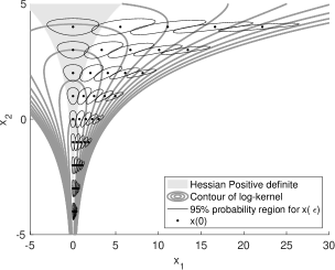
Figure 1: Illustration of the effect of modified Cholesky manifold scaling on RMHMC proposals for the bivariate funnel distribution (11). The MCRMHMC uses the tuning parameters $K=1,u_{2}=1.0,$ $\varepsilon=0.15$. Only the right half-plane is considered due to symmetry. Contours of the log-target (11) are indicated by grey lines. Dots indicate initial states $\mathbf{x}(0)$ and closed black curves indicate corresponding 95% probability regions for $\hat{\mathbf{x}}(\varepsilon)|\mathbf{x}(0)$. The negative Hessian $-\nabla_{\mathbf{x}}^{2}\log\tilde{\pi}(\mathbf{x})$ is positive definite in the region shaded with light gray. Note that corresponding 95% probability region curves for EHMC methods (such as the Stan NUTS) would have the same (elliptical) shape for all initial states.

To illustrate the proposed methodology, consider a bivariate version of the Neal (2003) funnel distribution, given as

$$\log\tilde{\pi}(\mathbf{x})=-\frac{x_{1}^{2}}{2\exp(x_{2})}-\frac{x_{2}}{2}-\frac{x_{2}^{2}}{18}.$$ (11)

Namely, $x_{1}|x_{2}\sim N(0,\exp(x_{2}))$, $x_{2}\sim N(0,3^{2})$. This model displays substantially different scales in $x_{1}$ depending on the value of $x_{2}$, and therefore illustrates how joint sampling of variables along with the variance parameter of these variables (e.g. latent field and the variance of the latent field) poses substantial problems for MCMC methods that do not adapt to local scaling properties.

Methods based on mode and (negative inverse) Hessian at the mode (Gelman et al., 2014, Chapter 13.3) for scaling MCMC proposals are not reliable for such targets. I.e. the target has mode at $\left[0,-4.5\right]^{T}$ whereas $E(\mathbf{x})=\left[0,0\right]^{T}$. The negative inverse Hessian at the mode variance approximation yields $\text{diag}(0.0111,9)$ whereas $Var(\mathbf{x})=\text{diag}(90.01,9).$ It is seen that the mode is shifted in the $x_{2}$-direction toward the smaller scale region (negative $x_{2}$) as smaller scales yield higher values of $p(x_{1}|x_{2})$. The variance in $x_{1}$-direction indicated by the inverse negative Hessian at the mode is also very different from $Var(x_{1})$, but one can argue that none of these variances are very informative for globally scaling MCMC proposals due to the different scales in $x_{1}$-direction determined by $x_{2}$.

Since $x_{1}|x_{2}$ is Gaussian, it is clear that
$(-\nabla_{\mathbf{x}}^{2}\log\tilde{\pi}(\mathbf{x}))_{1,1}>0$, and therefore $K=1$ is used to implement MCRMHMC for this model. Figure 1 shows 95% probability regions for single (time integration) step proposals of MCRMHMC, for a selection of initial configurations (indicated by dots) for target (11). It is seen that the metric tensor of MCRMHMC appropriately scales the proposals and aligns the proposal distributions to the local geometry of the target. The negative Hessian is positive definite only in region shaded with light gray ($x_{1}\in(\mp(\sqrt{2}/3)\exp(x_{2}/2))$), and it is seen that the negative Hessian in conjunction with the modified Cholesky factorization also produces useful scale information when the Hessian is indefinite. This latter observation is very much in line with the numerical optimization literature on modified Newton methods (Nocedal and Wright, 1999, Chapter 6). Moreover, due to the relatively high degree of regularisation in the $x_{2}$-direction ($u_{2}=1.0$), no problems related to close to zero eigenvalues near boundaries of the shaded region are seen (Kleppe, 2016).

3.4 Discussion of the modified Cholesky factorization

Several issues related to the modified Cholesky factorization in Algorithm 1 and its application in the RMHMC context require further clarification at this point. First, it is clear that Algorithm 1 is not invariant to reordering of the variables in $\mathbf{x}$, a property that is often imposed in optimisation contexts via symmetric row and column interchanges (Gill et al., 1981; Nocedal and Wright, 1999). Such row and column interchanges are not applied here as they 1) introduce discontinuities in $\nabla_{\mathbf{x}}H$ which in turn makes simulating the flow associated with (2,3) more difficult, 2) disturb any exploitation of $(K\times K$) positive definite upper left sub-matrices, 3) make exploitation of sparsity of the negative Hessian substantially less effective as the sparsity pattern of the modified Cholesky factorizations changes. Moreover, a further rationale for including such symmetric row- and column interchanges is to avoid numerical instabilities associated with small finalized $D_{j,j}$s, but in the present context such problems can be tuned away by appropriate increases in $u_{j}$.

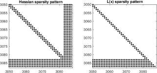
Figure 2: Sparsity patterns for the log-target Hessian and its associated modified Cholesky factor $L(\mathbf{x})$ for the model considered in Section 5. Non-zero elements are indicated by dots. In order to improve readability, only the lower right (3050:3087,3050:3087) submatix is shown in both cases. The patterns repeats along the borders and (sub,sup)-diagonals in the complete matrices. For the Hessian, only 0.4% of the elements are non-zero, whereas only 0.5% of the lower triangular elements of $L(\mathbf{x})$ are non-zero.

Given that Algorithm 1 is not invariant to reordering of variables, it reasonable to ask what is an appropriate ordering of the variables? The short answer is that this is a tradeoff between exploiting any possible positive definite sub-matrices by putting the associated variables first in $\mathbf{x}$, and using orderings of the variables so that $L(\mathbf{x})$ is as sparse as possible (Davis, 2006). Fortunately, in the context of hierarchical models and especially for LGMs, the means to these two objectives often align well, in the sense that the latent vector, conditional on parameters, often is both associated with a positive definite negative Hessian and (possibly after an appropriate internal reordering using e.g. the AMD algorithm of Davis, 2006, Chapter 7) has a Cholesky factorization with exploitable sparsity structure (see Rue et al., 2009, where both of these properties are exploited in the LGM context in the Laplace approximation used for calculating marginal posteriors of the parameters). Thus, assuming the above situation, a rule of thumb will be to put the latent variables first in $\mathbf{x}$ and let the last elements of $\mathbf{x}$ be the parameters. This strategy leads to the rows of $L(\mathbf{x})$ corresponding to the latent variables being sparse, and the remaining (typically few) rows corresponding to parameters being dense. To illustrate this rule of thumb procedure, Figure 2 displays the sparsity patterns of the log-target negative Hessian and associated Cholesky factor $L(\mathbf{x})$ for the non-linear state space model discussed in detail in Section 5. The model consists of $3082$ latent variables with first order (time series) Markov structure (put first in $\mathbf{x}$), and 5 parameters (put last in $\mathbf{x}$). Due to the Markovian structure, the sub-matrix corresponding to the latent variables is tri-diagonal, and consequently the Cholesky factor has only non-zero elements on the diagonal and the first sub-diagonal. This property is retained for the Cholesky factor of the complete negative Hessian, where only the rows corresponding to the parameters are dense.

A discussion of the vector of regularisation parameters $\mathbf{u}$ is also in order. Recall that Algorithm 1 requires $d-K$ regularisation parameters, where the $\left\{u_{j}\right\}_{j=K+1}^{d}$ should reflect the potentially very different scaling of $\left\{x_{j}\right\}_{j=K+1}^{d}$. Including a potentially large number of regularisation parameters naturally comes both with added flexibility and potential for very high-fidelity sampling when tuned properly. On the other hand, including many regularisation parameters may lead to time-consuming tuning efforts, in particular since the interpretation of $\left\{u_{j}\right\}_{j=K+1}^{d}$ is not as straight forward as in the softmax metric based on full spectral decompositions (Betancourt, 2013a). Though, of course, all active regularisation parameters can be set equal, and thus reduce to a single regularisation parameter as is the case in the softmax metric of Betancourt (2013a), in many cases this may lead to suboptimal sampling in a RMHMC context as unnecessary regularisation will lead to slower and more oscillating exploration of the target.

To further illustrate the advantages of this regularisation scheme, consider the toy model discussed in detail in Section 4.2, consisting of a Gaussian zero mean AR(1) model with autocorrelation 0.999 as $\mathbf{x}_{1:d-1}$, and let $x_{d}$ be the logarithm of the innovation precision of said AR(1) model. For $d=1000$, $x_{d}=-3.0$ and $\mathbf{x}_{1:d-1}$ simulated from the true model, the eigenvalues of the negative Hessian are (in ascending order) $(-0.067,\;1.35e-7,\;7.22e-7,\dots)$, whereas the eigenvalues of the negative Hessian associated with $\mathbf{x}_{1:d-1}$ are $(1.35e-7,\;7.22e-7,\dots)$. Given that $\mathbf{x}_{1:d-1}$ is jointly Gaussian, the negative Hessian of $\mathbf{x}_{1:d-1}$ is by construction positive definite, but with smallest eigenvalue several orders of magnitude smaller than the absolute value of the single negative eigenvalue associated with $\mathbf{x}$. The modified Cholesky approach, with $K=d-1$, will exactly reproduce the precision matrix of $\mathbf{x}_{1:d-1}$ in $G_{1:d-1,1:d-1}$ and only apply regularisation in the dimension corresponding to the log-precision parameter. Regularisation in eigen-space, on the other hand, is likely to disturb the representation of the precision matrix of $\mathbf{x}_{1:d-1}$ in $G$ substantially, as it is likely that regularisation at least a few orders of magnitude smaller than the negative eigenvalue needs to be applied. The disturbed representation of these eigenvalues will lead to less efficient sampling as the resulting RMHMC algorithm will to a lesser degree align the Hamiltonian dynamics with the strong dependence among $\mathbf{x}_{1:d-1}$.

3.5 Implementation and tuning

The prototype large scale code used in the reminder of this paper is implemented in C++ and uses a sparsity-exploiting implementation of Algorithm 1 that is derived from the function cs_chol of the csparse library (Davis, 2006). Since the sparsity pattern of $L$ is identical to that of a conventional sparse Cholesky factorization, the functions of the csparse library for calculating sparsity patterns, speeding up computations (elimination trees) and other numerical tasks such as triangular solves can be used directly.

The code makes use of the template capabilities of the C++ language so that a single code is maintained both for double numerics for calculating $H$ and $\nabla_{\mathbf{p}}H$, and with automatic differentiation (AD) types for calculating $\nabla_{\mathbf{x}}H$. Specifically, the AD tool adept (Hogan, 2014) is used for the latter task. Finally, in the current version, $-\nabla_{\mathbf{x}}^{2}\log\tilde{\pi}(\mathbf{x})$ is hand-coded. However, in future versions, this task will also be automated using AD-software capable of exploiting the sparsity of the Hessian (Griewank, 2000).

As discussed above, the methodology involves a number of tuning parameters, which need to be adjusted for each particular target distribution. Here, a method for such adjustment during a warm up phase is provided, which has been used for the computations described in the reminder of the paper. Firstly, the ordering of variables and selection of $K$ is done mainly based on insight into the problem at hand, with $K$ latent variables typically taken first in $\mathbf{x}$, and parameters, in particular scales and correlations, put last in $\mathbf{x}$. Subsequently, too high initial guesses of $K$ can be reduced to $j-1$ during warm up if $D_{j,j}<0,$$j\leq K$ at step 4 of Algorithm for some $\mathbf{x}$. If such a situation is encountered during the post-warm up phase, the MCMC simulation needs to be restarted with reduced $K$.

Secondly, the joint tuning of $\varepsilon$, $l$ and $\left\{u_{j}\right\}_{j=K+1}^{d}$ requires some more attention. The heuristic strategy adopted here is based on the following three steps:

• Select some reference $\varepsilon$ and $l$, e.g. $\varepsilon=0.5d^{-0.25}$ and $E(l)=\lfloor 1.5/\varepsilon\rfloor$. The expressions for $\varepsilon$, $l$ are informed firstly by the fact that for any Gaussian target, say $N(\mu,\Sigma)$, then $G(\mathbf{x})=\Sigma^{-1}$ and the integrator (5-8) reduces to the conventional leap frog integrator for separable Hamiltonian systems. In this situation, it is known that an asymptotic expression for the expected acceptance probabilities for proposals independent of current configuration ($\varepsilon l\approx\pi/2)$ is $2-2\Phi(\varepsilon^{2}\sqrt{d}/8)$ (see e.g. Beskos et al., 2013; Mannseth et al., 2017), which when solved for $\varepsilon$ with acceptance probability 0.95 yields $\varepsilon\approx 0.7d^{-0.25}$. In practice, it is usually the case that slightly smaller values of $\varepsilon$ are needed for models with non-constant curvature and hence $\varepsilon=0.5d^{-0.25}$ is taken as a reasonable step size. Secondly, the reference expression for the number of integration steps is informed by the $l\varepsilon\approx\pi/2$ needed in the Gaussian case, whereas the connection to Newton’s method in optimization indicates $l\varepsilon\approx\sqrt{2}$.

• Tune $\left\{u_{j}\right\}_{j=K+1}^{d}$ using the reference values of $\varepsilon$ and $l$, with the objective of taking $\left\{u_{j}\right\}_{j=K+1}^{d}$ as small as possible while ensuring the Hamiltonian is well-behaved enough for the fixed point iterations associated with (6-7) to converge. In practice, this tuning is implemented by initially setting each active $u_{j}$ to a small number, say $\exp(-20)$, to avoid unnecessary and computationally wasteful regularisation, and run a number of warm up iterations while increasing the relevant $u_{j}$ by a factor say $\exp(1)$ whenever a divergence in the fixed point iterations is encountered. Divergences in the fixed point iterations for both (6) and (7) indicate that $\|J(\mathbf{x},\mathbf{p})\|>1$ where $J(\mathbf{x},\mathbf{p})=\frac{\varepsilon}{2}\nabla_{\mathbf{x},\mathbf{p}}^{2}H(\mathbf{x},\mathbf{p})=\frac{\varepsilon}{2}\nabla_{\mathbf{x}}[G^{-1}(\mathbf{x})\mathbf{p}]$ around the sought fixed point. Moreover, for small $|D_{j,j}|/u_{j}$ (relative to say 10) and small $u_{j}$, $\frac{d}{dz}[\text{sabs}(z;u_{j})]^{-1}|_{z=D_{j,j}}$ contributes substantially to $\|J(\mathbf{x},\mathbf{p})\|$ and an ideal approach for choosing which $u_{j}$ to increase would be to measure the sensitivity of $\|J(\mathbf{x},\mathbf{p})\|$ to each of the active $u_{j}$s. Rather than computing the norm of the complete Jacobian, a heuristic approach is taken, which involves increasing $u_{\hat{j}}$ for
  $\hat{j}=\arg\max_{K<j\leq d}|\frac{d}{dz}[\text{sabs}(z;u_{j})]^{-1}|_{z=D_{j,j}}|$ whenever a divergence is detected. It is worth noticing that, in failing to take into account the sensitivity of the negative Hessian on $\mathbf{x}$ and the fact that $D_{j,j}$ is also used in subsequent iterations in Algorithm 1, this approach is likely to be suboptimal with respect to selecting the relevant $u_{j}$. This is in particular the case when the target under consideration contains strong dependencies, and thus basing such a selection mechanism on a more direct approximation to $\|J(\mathbf{x},\mathbf{p})\|$ is scope for future research.

• Tune $\varepsilon$ and $l$ for fixed $\left\{u_{j}\right\}_{j=K+1}^{d}$, with the objective of controlling the acceptance probability and producing low-autocorrelation samples using standard procedures. In particular, this part of the tuning is readily automated using dynamic selection of $l$ (Betancourt, 2013b; Hoffman and Gelman, 2014; Betancourt, 2016) and tuning $\varepsilon$ toward a given acceptance probability e.g. using the dual averaging algorithm of Hoffman and Gelman (2014).

4 Simulation study

To benchmark the proposed methodology against common, general purpose MCMC methods, two challenging toy models are considered. These exhibit, in the first case, strong non-linear dependence, and in the second case, a “funnel” effect. The contending methods are chosen as they are routinely used in diverse high-dimensional applications. Throughout this section, all methods except Stan were implemented in C++ and compiled with the same compiler, and with the same compiler settings. The Stan computations were done using the R-interface rstan, version 2.15.1, running under R version 3.3.3. The computer used for all computations in this section was a 2014 Macbook Pro with a 2.0 GHz Intel Core i7 processor.

4.1 Twisted Gaussian mean AR(1) model

Method	# MCMC	CPU time		$\underset{1\leq i\leq d-1}{\min}ESS(x_{i})$		$ESS(x_{d})$		$\frac{\underset{1\leq i\leq d-1}{\min}ESS(x_{i})}{\text{CPU time}}$		$\frac{ESS(x_{d})}{\text{CPU time}}$
	iterations	(seconds)
Across replica		min	mean	min	mean	min	mean	min	mean	min	mean
$d=10$
MCRMHMC	1000	3.3	3.4	603	813	891	981	177	239	259	289
Gibbs	5000000	2.3	2.3	33	94	59	146	14	40	25	63
EHMC	5000	4.7	4.8	1056	1182	630	700	220	246	132	146
Stan	5000	1.4	1.4	(4312)	(4800)	(4465)	(4833)	(3137)	(3355)	(3144)	(3379)
EigenRMHMC	1000	425	432	59	93	59	96	0.14	0.21	0.14	0.22
$d=100$
MCRMHMC	1000	65	66	756	873	843	954	11	13	13	14
Gibbs	5000000	22	22	(7.2)	(24)	(9.6)	(26)	(0.32)	(1.1)	(0.43)	(1.2)
EHMC	5000	75	76	460	671	570	775	6.0	8.8	7.6	10
Stan	5000	12	14	(4648)	(4868)	(4531)	(4870)	(315)	(349)	(324)	(349)
$d=1000$
MCRMHMC	1000	1435	1456	451	723	728	879	0.31	0.50	0.50	0.60
Gibbs	5000000	223	224	(4.0)	(15)	(3.9)	(12)	(0.02)	(0.07)	(0.02)	(0.06)
EHMC	5000	1855	1897	46	214	90	268	0.02	0.11	0.05	0.14
Stan	5000	225	255	(4529)	(4786)	(4607)	(4852)	(17)	(19)	(17)	(19)

Table 1: Results for the twisted Gaussian mean AR(1) model experiment. Each combination of method and $d\in\{10,100,1000\}$ was repeated 10 independent times and the numbers presented are minimum (min) and means (mean) across these replica. Visual inspection of output (Figures 3 - 5) and Kolmogorov-Smirnov tests (applied for MCRMHMC and Stan) indicate that some samplers failed to explore the relevant support, and the corresponding numbers are given in parentheses. The results for the Gibbs sampler are only recorded every 1000th iteration, thus the maximum ESSs for Gibbs are 5000. Tuning parameters for MCRMHMC are: $d=10$: $u_{n}=\exp(3.5),\varepsilon=0.4,l\sim U(20,30)$, $d=100$: $u_{n}=\exp(3.5),\varepsilon=0.15,l\sim U(60,80)$, $d=1000$: $u_{n}=\exp(3.5),\varepsilon=0.1,l\sim U(130,160)$. For Gibbs, tuning parameters are: $d=10$: $r_{Gibbs}=0.65$, $d=100$: $r_{Gibbs}=0.4$ and $d=1000$: $r_{Gibbs}=0.05$. For EHMC, tuning parameters are: $d=10$: $\varepsilon=0.02,l\sim U(700,1000)$, $d=100$: $\varepsilon=0.01,l\sim U(1500,2000)$, and $d=1000$: $\varepsilon=0.007,l\sim U(4000,6000)$. Finally for EigenRMHMC, $d=10$: $u=\exp(3)$, $\varepsilon=0.3$ and $l\sim U(50,100)$.

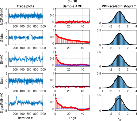
Figure 3: Traceplots (left), sample autocorrelation functions (center) and pdf-scaled histograms (right) of MCMC iterations for $x_{d}$ for $d=10$. Under target characterized by (12-14), $x_{d}$ has a standard Gaussian marginal distribution, which is indicated as a reference for the histograms.

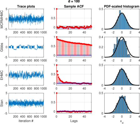
Figure 4: Traceplots (left), sample autocorrelation functions (center) and pdf-scaled histograms (right) of MCMC iterations for $x_{d}$ for $d=100$. Under target characterized by (12-14), $x_{d}$ has a standard Gaussian marginal distribution, which is indicated as a reference for the histograms.

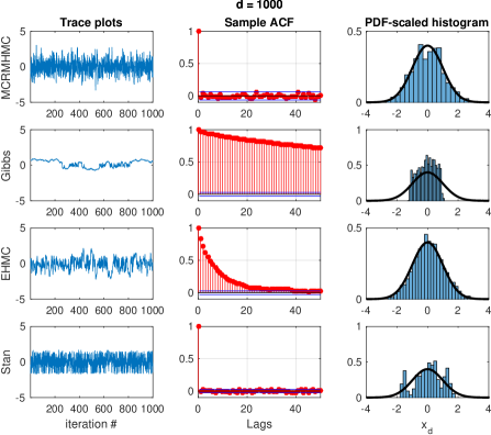
Figure 5: Traceplots (left), sample autocorrelation functions (center) and pdf-scaled histograms (right) of MCMC iterations for $x_{d}$ for $d=1000$. Under target characterized by (12-14), $x_{d}$ has a standard Gaussian marginal distribution, which is indicated as a reference for the histograms.

This first toy model is given by

$$x_{i}|x_{i-1},x_{d}\\ \sim N\left((x_{d}^{2}-1)+0.95(x_{i-1}-(x_{d}^{2}-1)),\frac{1-0.95^{2}}{100}\right),\\ \;i=2,\dots,d-1,$$ (12)

$$x_{1}|x_{d} \sim N\left(x_{d}^{2}-1,\frac{1}{100}\right),$$ (13)

$$x_{d} \sim N(0,1).$$ (14)

I.e. conditionally on $x_{d}$, $\mathbf{x}_{1:d-1}$ is a Gaussian AR(1) process with autocorrelation 0.95, marginal standard deviation 0.1 and mean $x_{d}^{2}-1$. Similar specifications, but without autocorrelation, have previously been considered as test cases for MCMC algorithms (Haario et al., 1999; Betancourt, 2013b). The model may be considered as a very simple hierarchical model, where $\mathbf{x}_{1:d-1}$ are latent variables, $x_{d}$ is a parameter, and no observations are modelled (in order to retain analytical marginals).

The contending methods are chosen as they share scope with respect to generality. Specifically, Gibbs sampling, EHMC with identity mass matrix, Stan and RMHMC using full spectral decomposition (EigenRMHMC) similar to Betancourt (2013a), in addition to the proposed methodology were considered. The Gibbs sampler (Gibbs) was implemented using single dimension updates in order to mimic a situation where $\mathbf{x}_{1:d-1}$ are latent variables with intractable joint conditional posterior. Specifically, for updating $x_{i}|\mathbf{x}_{-i},\;i=1,\dots,d-1$, exact Gaussian updates were used. For updating $x_{d}|\mathbf{x}_{1:d-1}$, a Gaussian random walk Metropolis Hastings method, with proposal standard deviation $r_{Gibbs}$ was used. Here, $r_{Gibbs}$ was tuned to produce update rates of 20-30%. Due to the slow mixing, but low per iteration computational cost, only every 1000th Gibbs iteration was recorded.

For EHMC, uniformly distributed numbers of time integration steps $l$ were used, where the notation $U(a,b)$ denotes uniform on the integers between $a$ and $b$ including $a,b$. In addition, the integration step sizes were jittered with $\pm 15\%$ uniform noise (Neal, 2010). The distributions for $l$ and $\varepsilon$ were tuned to target an acceptance rate around 60% and to produce MCMC samples that were well separated in the $x_{n}$-direction.

Stan was run using 10000 iterations, where the first 5000 (warm-up) iterations were used for tuning the sampler. The diag_e metric (i.e. general fixed diagonal scaling matrix) and otherwise default settings were used. The warm-up iterations are not included in the reported CPU times.

The negative Hessian of the log-density of $\mathbf{x}_{1:d-1}|x_{d}$ is positive definite, which enables $K=d-1$ for
MCRMHMC. The sparsity patterns of the negative Hessian and modified Cholesky factor $L$ are similar to those of Figure 2 with the exception that this model only has one “parameter” with corresponding dense $d$th row in Hessian and $L$. The values for $u_{d}$ were found by successively increasing $u_{d}$ until the iterative solvers in the time integrator no longer diverged for a reference value of $\varepsilon$. Also here, uniformly distributed numbers of time integration steps and $15\%$ jittered step sizes were used. The integration step size was taken to produce acceptance rates of around 95% and the tuning of the distribution of $l$ was again taken to produce high fidelity samples for $x_{d}$.

EigenRMHMC was implemented using full spectral decomposition, followed by applying the sabs-function (see Algorithm 1) with parameter $u$ to each eigenvalue to produce a positive definite metric tensor. Other than the metric tensor, MCRMHMC and EigenRMHMC are identical. In particular $u$ was tuned by increasing $u$ until the iterative solvers no longer diverged and the integration step size was tuned toward acceptance rates around 95%. For both MCRMHMC and EigenRMHMC, AD was applied to the complete code (i.e. including modified Cholesky factorization- and spectral factorization codes).

The experiment was run for each of $d\in\{10,100,1000\}$. EigenRMHMC was only considered in the $d=10$ case, as very long computing times were required in higher dimensions. In all considered cases, each method was run 10 independent times. For each method except Stan, realizations from the target distribution were used as initial values for the MCMC methods, and therefore no warm up iterations were performed. To compare the performances of the MCMC methods, the effective sample size (ESS), calculated using the monotone sample autocorrelation estimator of Geyer (1992) was employed.

The results are presented in Table 1, and trace plots, sample autocorrelation functions and histograms for $x_{d}$ are presented in Figures 3 - 5. First, it is seen from Figures 3 - 5 that the Gibbs sampler, even after 5 million iterations, fail to properly explore the target distribution. Also Stan seem to produce samples that do not fully explore the target distribution, which is seen most clearly from Figure 5. Due to the close to zero autocorrelation of the Stan and MCRMHMC MCMC samples, Kolmogorv-Smirnov tests with null hypothesis being that samples representing $x_{d}$ are standard normal were conducted. The null hypothesis is strongly rejected for Stan in all cases, whereas not rejected for MCRMHMC in all cases. Thus, only MCRMHMC, EHMC and EigenRMHMC appear to produce accurate representations of the target distribution, with MCRMHMC producing uniformly highest ESSes and ESSes per computing time for $d=100,1000$, both in minimum and mean across replica. Moreover, the relative ESS per CPU time for MCRMHMC and EHMC appears to increase with increasing dimension, with MCRMHMC being a factor 4 faster for $d=1000$. Further, visual inspection of the Hamiltonian dynamics trajectories (unreported) shows a very coherent and fast exploration of the target by the MCRMHMC, whereas the trajectories of EHMC and EigenRMHMC are oscillating due to the strong dependency structure, and therefore lead to a slow exploration of the target. In the case of EigenRMHMC, it seems the regularisation parameter needed to make the fixed point iterations of integrator converge also strongly influences the representation of the AR(1) model precision in the implied $G(\mathbf{x})$, which slows down the exploration.

4.2 Funnel AR(1) model

The second toy model considered is a zero mean Gaussian AR(1) model with autocorrelation $0.999$ jointly with the innovation precision parameter, where the latter has a gamma(1,0.1) prior:

$$x_{i}|x_{i-1},x_{d}\sim N\left(0.999x_{i-1},\frac{1}{\exp(x_{d})}\right),\\ \;i=2,\dots,d-1,$$ (15)

$$x_{1}|x_{d} \sim N\left(0,\frac{1}{\exp(x_{d})(1-0.999^{2})}\right),$$ (16)

$$\exp(x_{d}) \sim\text{gamma}(1,0.1).$$ (17)

This model exhibit a “funnel” nature (Neal, 2003; Betancourt, 2013b) as the marginal standard deviation of $x_{i},\;i=1,\dots,d-1$ varies by two orders of magnitude between the $0.001$ and $0.999$ quantiles of $x_{d}$. Moreover, there is a very strong dependence among $x_{i},\;i=1,\dots,d-1$ which adds further complications for many MCMC methods. Thus, also this target distribution shares many of the features of the (joint latent variables and parameters) target distribution associated with hierarchical models.

Method	# MCMC	CPU time		$\underset{1\leq i\leq d-1}{\min}ESS(x_{i})$		$ESS(x_{d})$		$\frac{\underset{1\leq i\leq d-1}{\min}ESS(x_{i})}{\text{CPU time}}$		$\frac{ESS(x_{d})}{\text{CPU time}}$
	iterations	(seconds)
Across replica		min	mean	min	mean	min	mean	min	mean	min	mean
$d=10$
MCRMHMC	1000	6.1	6.1	622	912	928	987	101	149	152	161
Gibbs	5000000	2.3	2.4	588	698	1295	1613	250	297	548	686
EHMC	5000	6.3	6.5	(8.9)	(48)	(20)	(161)	(1.4)	(7.3)	(3.2)	(25)
Stan	5000	4.0	5.4	(4627)	(4839)	(4534)	(4856)	(692)	(918)	(704)	(920)
EigenRMHMC	1000	1640	1694	17	56	32	76	0.01	0.03	0.02	0.04
$d=100$
MCRMHMC	1000	154	156	482	628	398	533	3.1	4.0	2.6	3.4
Gibbs	5000000	20	20	(42)	(76)	(111)	(243)	(2.1)	(3.8)	(5.5)	(12)
EHMC	5000	89	91	(5.4)	(11)	(8.4)	(33)	(0.06)	(0.12)	(0.09)	(0.36)
Stan	5000	33	42	(4455)	(4742)	(4537)	(4844)	(92)	(114)	(96)	(116)
$d=1000$
MCRMHMC	1000	11778	11927	331	636	596	908	0.03	0.05	0.05	0.08
Gibbs	5000000	198	198	(5.9)	(15)	(7)	(49)	(0.03)	(0.08)	(0.03)	(0.25)
EHMC	5000	1686	1708	(3.1)	(3.4)	(4.6)	(10)	(0.002)	(0.002)	(0.003)	(0.006)
Stan	5000	487	511	(3718)	(4391)	(3976)	(4776)	(6.8)	(8.7)	(6.7)	(9.5)

Table 2: Results for the funnel AR(1) model (Equations 15-17) experiment. Each combination of method and $d\in\{10,100,1000\}$ was repeated 10 independent times and the numbers presented are minimum (min) and means (mean) across these replica. Visual inspection of output (Figures 6 - 8) and Kolmogorov-Smirnov tests (applied for MCRMHMC and Stan) indicate that some samplers failed to explore the relevant support, and the corresponding numbers are given in parentheses. The results for the Gibbs sampler are only recorded every 1000th iteration, thus the maximum ESSs for Gibbs are 5000. Tuning parameters for MCRMHMC are: $d=10$: $u_{d}=\exp(2.0),$ $\varepsilon=0.3$, $l\sim U(30,40)$, $d=100$: $u_{d}=\exp(2.5),$ $\varepsilon=0.15$, $l\sim U(110,130)$ and $d=1000$: $u_{d}=\exp(3.0),$ $\varepsilon=0.075$, $l\sim U(1100,1300)$. Tuning parameters for EHMC are $d=10$: $\varepsilon=0.05,$ $l\sim U(1000,1500)$, $=100$: $\varepsilon=0.025$, $l\sim U(2000,3000)$ and $d=1000$: $\varepsilon=0.001$, $l\sim U(4000,6000)$. For Stan, default tuning parameters, except adapt_delta = 0.999 were used. Tuning parameters for EigenRMHMC are $d=10$: $u=\exp(-1.0)$, $\varepsilon=0.3$ and $l\sim U(200,300)$.

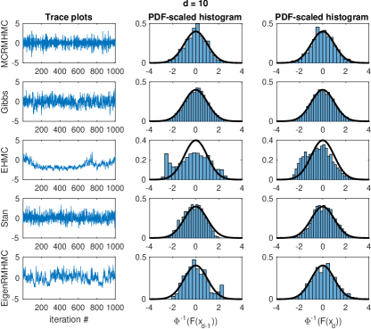
Figure 6: Trace plots and histograms for the funnel AR(1) model experiment, $d=10$. Left column displays trace plots of $\Phi^{-1}(F_{x_{d}}(x_{d}))$, which should have a standard Gaussian distribution. The middle column displays density-scaled histograms of $\Phi^{-1}(F_{x_{d-1}}(x_{d-1}))$, along with a standard Gaussian density. The right column displays density-scaled histograms of $\Phi^{-1}(F_{x_{d}}(x_{d}))$ along with a standard Gaussian density.

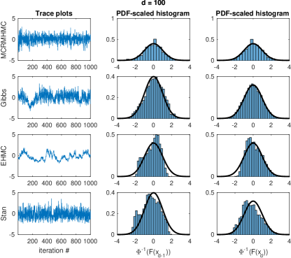
Figure 7: Trace plots and histograms for the funnel AR(1) model experiment, $d=100$. Left column displays trace plots of $\Phi^{-1}(F_{x_{d}}(x_{d}))$, which should have a standard Gaussian distribution. The middle column displays density-scaled histograms of $\Phi^{-1}(F_{x_{d-1}}(x_{d-1}))$, along with a standard Gaussian density. The right column displays density-scaled histograms of $\Phi^{-1}(F_{x_{d}}(x_{d}))$ along with a standard Gaussian density.

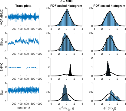
Figure 8: Trace plots and histograms for the funnel AR(1) model experiment, $d=1000$. Left column displays trace plots of $\Phi^{-1}(F_{x_{d}}(x_{d}))$, which should have a standard Gaussian distribution. The middle column displays density-scaled histograms of $\Phi^{-1}(F_{x_{d-1}}(x_{d-1}))$, along with a standard Gaussian density. The right column displays density-scaled histograms of $\Phi^{-1}(F_{x_{d}}(x_{d}))$ along with a standard Gaussian density.

Also here, four alternatives to the proposed methodology were considered, namely Gibbs sampling, EHMC, Stan and EigenRMHMC (only for $d=10$). The model allows for a full set of univariate conditional posteriors with standard distributions, which are applied in the Gibbs sampler. For the Gibbs sampler, only every 1000th iteration was recorded due to the very slow mixing. Also here, the Euclidian metric HMC was implemented using an identity mass matrix. Due to the substantial “funnel” nature of the target, the integrator step size for EHMC must be chosen quite small to be able to explore the low-variance region of the target, which in turn leads to very high acceptance probabilities (Betancourt, 2013a). However, finding a reasonable distribution for $l$ that simultaneously leads to MCMC samples with low autocorrelation seems impossible. Also for Stan, small step sizes were imposed to account for differences in scales via setting the acceptance rate target adapt_delta equal to 0.999. For MCRMHMC, again $\mathbf{x}_{1:d-1}|x_{d}$ is Gaussian which suggest $K=d-1$, and the sparsity structure and tuning strategy is identical as for the model in Section 4.1. For EigenRMHMC, again the regularisation parameter $u$ was chosen in order to produce few divergences in the integrator fixed point iterations. However, for this $u$, it appears that the regularisation interferes with representation of the AR(1) process precision, and thus precludes finding small values of $l$ that produce high fidelity samples (see Section 3.4). The applied values of $l$ are larger than those required for MCRMHMC. The experimental setup is otherwise identical to that of Section 4.1.

Due to the simple structure of the target, it is clear that the marginal cumulative distribution functions of $x_{i}$, say $F_{x_{i}}$, are easily determined from $\exp(x_{d})\sim\text{gamma}(1,0.1)$ and $\sqrt{0.1(1-0.999^{2})}x_{i}\sim t_{2}$,
$i=1,\dots,d-1$. This information can be exploited to determine the quality of the convergence for the different methods. Results from the simulation experiment for $d\in\{10,100,1000\}$ are presented in Table 2 and Figures 6 - 8. Looking first at Figures 6 - 8, where the middle and right columns present density-scaled histograms of the MCMC output for a representative replica, transformed to have standard Gaussian marginal distribution via the $\Phi^{-1}\circ F_{x_{i}}$ transformation for $x_{d-1}$ and $x_{d}$ respectively. Firstly, it is seen that EHMC, even with very large $E(l)$ and very high acceptance rates, is unable to fully explore the target for all considered $d$s for this model. Secondly, this appears also to be the case for the Gibbs sampler for $d=100,1000$. Also Stan fails to explore the target fully (most easily seen in Figures 7, 8), and Kolmogorov-Smirnov tests reject that the Stan MCMC samples come from the true marginals in all cases. From Table 2 it is seen that MCRMHMC produces high-fidelity samples in all cases, but that in the $d=10$ case, Gibbs sampling produces effective samples faster than MCRMHMC. EigenRMHMC is four orders of magnitude slower than MCRMHMC and Gibbs in the $d=10$ case.

Overall, the simulation studies for models (12-14) and (15-17) indicate that MCRMHMC is capable of producing reliable results for challenging models with diverse forms of non-linearities and strong dependencies structures. On the other hand, the contending methods may require prohibitively long MCMC chains to accurately represent the target distribution. Having said that, one can argue that the conditional Gaussian AR(1) models in (12-14) and (15-17) pose too small challenges for MCRMHMC. Therefore, also a non-linear state space model where the prior for the latent variables is far from jointly Gaussian is considered.

5 Application to a state space model

In this section, a Euler-Maruyama-discretized version of the Chan et al. (1992) constant elasticity of variance model for short term interest rates, observed with Gaussian noise, is considered. The model is fully specified by

$$y_{t}=x_{t}+\sigma_{y}\eta_{t},\;\eta_{t}\sim i.i.d.\;N(0,1),\;t=1,\dots,T,$$ (18)

$$x_{t}=x_{t-1}+\Delta(\alpha-\beta x_{t-1})+\sigma_{x}\sqrt{\Delta}x_{t-1}^{\gamma}\varepsilon_{t},\\ \;\varepsilon_{t}\sim i.i.d.\;N(0,1),\;t=2,\dots,T$$ (19)

$$x_{1}\sim N(0.09569,0.01^{2}),$$ (20)

where $\Delta=1/252$ correspond to a daily sampling frequency for a yearly time scale. Here $\mathbf{x}_{1:T}$ models an unobserved short term interest rate, which is observed with noise in $\mathbf{y}_{1:T}$. The prior mean of $x_{1}$ is set equal to the first observation $y_{1}$. Due to the non-constant volatility term in the $x_{t}$ process, the joint prior for $\mathbf{x}_{1:T}$ deviates strongly from being Gaussian. The model is completed with the following, (improper) prior assumptions and transformations to prepare for MCRMHMC sampling:

$$x_{T+1} =\alpha\sim N\left(0,\frac{100}{\Delta^{2}}\right),$$

$$x_{T+2} =\beta\sim N\left(\frac{1}{\Delta},\frac{100}{\Delta^{2}}\right),$$

$$x_{T+3} =\log(\sigma_{x}^{2})\sim\text{uniform}(-\infty,\infty),$$

$$x_{T+4} =\gamma\sim\text{uniform}(0,\infty),$$

$$x_{T+5} =\log(\sigma_{y}^{2})\sim\text{uniform}(-\infty,\infty),$$

(the priors for $\alpha,\beta$ correspond to $N(0,100)$ priors on $\alpha^{\prime},\beta^{\prime}$ in the parameterization $E(x_{t}|x_{t-1})=\alpha^{\prime}+\beta^{\prime}x_{t-1}$). The dataset considered was $T=3082$ observations of 7-day Eurodollar deposit spot rates from January 2, 1983 to February 25, 1995. The dataset has previously been used in Aït-Sahalia (1996) and, in the context of model (18-20), in Grothe et al. (2016). To implement MCRMHMC with $d=T+5$, it is first observed that even though $p(x_{1:T}|x_{T+1:T+5})$ is not uniformly log-concave, it appears that $K=T+2$ is a suitable choice since the observations are highly informative with respect to the latent process, and further that $\alpha,\beta$ interacts only linearly with $\mathbf{x}_{1:T}$. The remaining active regularisation parameters were taken to be $u_{T+3}=\exp(6.0)$, $u_{T+4}=\exp(0.0)$, $u_{T+5}=\exp(6.0)$, which were determined using the heuristic detailed in Section 3.5. Moreover, $l\sim U(90,180)$ and $\varepsilon=0.03$ with 15% jittering of step size were used, which correspond to integration times ranging between $\approx 2.3$ and $\approx 6.2$. The applications of MCRMHMC were done using 1100 MCMC iterations where the 100 first iterations were discarded as warm up.

		MCRMHMC			Particle Gibbs
	CPU time (hours)	4.5			2.0
	# MCMC iterations	1000+100			80000+20000
	across replica	min	mean		min	mean
$\alpha$	Post. mean		0.0099			0.0098
	Post. std.		0.0088			0.0089
	ESS	1000	1000		36472	60801
	ESS/hour CPU time	222	224		17911	29755
$\beta$	Post. mean		0.168			0.168
	Post. std.		0.172			0.173
	ESS	1000	1000		56201	70998
	ESS/hour CPU time	222	224		27600	34752
$\sigma_{x}$	Post. mean		0.41			0.41
	Post. std.		0.06			0.06
	ESS	405	579		52	79
	ESS/hour CPU time	90	130		26	38
$\gamma$	Post. mean		1.18			1.19
	Post. std.		0.06			0.06
	ESS	423	564		53	78
	ESS/hour CPU time	94	127		26	38
$\sigma_{y}$	Post. mean		0.00054			0.00054
	Post. std.		2.3e-5			2.2e-5
	ESS	495	582		409	557
	ESS/hour CPU time	110	131		201	272
$x_{1}$	Post. mean		0.095			0.095
	Post. std.		0.0005			0.0005
	ESS	1000	1000		71512	73304
	ESS/hour CPU time	222	224		35087	35881
$x_{T}$	Post. mean		0.061			0.061
	Post. std.		0.0005			0.0005
	ESS	1000	1000		72415	74206
	ESS/hour CPU time	222	224		35519	36324

Table 3: Results for Bayesian inference for model (18-20) applied to a data set of Eurodollar interest rates with $T=3082$. Posterior mean and posterior standard deviation are denoted by Post. mean and Post. std. respectively. The numbers reported are the minimum (min) and mean (mean) across 10 independent replications of the experiments.

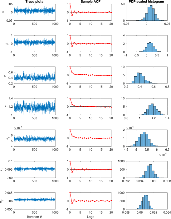
Figure 9: Trace plots, Sample autocorrelation functions and histograms for the CEV model (18-20) based on MCRMHMC. The reported plots are for a representative replica, and depicts only the 1000 post warm up samples.

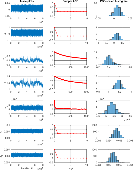
Figure 10: Trace plots, Sample autocorrelation functions and histograms for the CEV model (18-20) based on Particle Gibbs. The reported plots are for a representative replica, and depicts only the 80000 post warm up samples.

As a reference for the proposed methodology, a Particle Gibbs sampler (Andrieu et al., 2010) using the Particle EIS filter (Scharth and Kohn, 2016) with Ancestor Sampling (Lindsten et al., 2014) was used. This methodology is discussed in detail in Grothe et al. (2016) and should be regarded as a “state of the art” Gibbs sampling procedure for state space models where the latent state ($x_{1:T}$ in current notation) is updated in a single Gibbs block with close to perfect mixing. The Gibbs sampler was implemented fully in C++, and with a Gaussian random walk MH updating mechanism for $\gamma$ (with proposal standard deviation 0.025 corresponding to acceptance rates of 20-30%), but is otherwise identical to the one described in Grothe et al. (2016). A total of 100000 Gibbs iterations were performed, with the first 20000 iterations discarded as warm up. All experiments in this section were run on a 2016 iMac with a 3,1 GHz Intel Core i5 processor and 8 Gb of RAM, and each experiment was repeated 10 times using different random number seeds.

It is well known that Gibbs sampling for latent variable models often lead to poor mixing for the parameters determining the volatility of the latent process. This is at least partly due to “funnel”-like non-linear dependencies between the relevant parameters and the complete latent state. Thus, of particular interest is whether MCRMHMC is able to improve the sampling of these parameters by including both parameters and latents in the same updating block.

Results for MCRMHMC and Particle Gibbs sampling for the CEV model are presented in Table 3 and Figures 9 and 10. It is seen from Table 3 that both methods produce close to perfect sampling for parameters $\alpha,\;\beta,$ $x_{1},\;x_{T}$, and indeed also the other latents (not reported). However, for $\sigma_{x},\;\gamma$ and to some degree $\sigma_{y}$, the performance of the Particle Gibbs sampler deteriorates substantially, and for $\sigma_{x}$ and $\gamma$, MCRMHMC produces effective samples at a faster rate than the Particle Gibbs (both in mean and minimum across the replica). Thus, looking at the minimum (across $d$ dimensions) ESS per computing time, MCRMHMC performs better than Particle Gibbs, even if the Particle Gibbs updating mechanism for $\mathbf{x}_{1:T}$ is both fast and produces close to independent updates.

From Figure 9, it is seen that the samples from MCRMHMC explores the relevant support extremely fast for all dimensions, and it appears that only a few hundred iterations would be sufficient to produce a good representation of the joint posterior. A further, interesting artefact, is that for the conditionally log-concave latents/parameters ($\mathbf{x}_{1:T+2}$), the applied distributions for $l$ and $\varepsilon$ produce mildly negatively autocorrelated MCMC iterations, whereas there is a small positively correlated dependence for the parameters in need of regularisation ($\mathbf{x}_{T+3:T+5}$). This indicates that there is potentially scope for further improvement of the tuning of sampler, where it should be possible to align better the integration times needed to produce close to zero autocorrelation in all dimensions at the same time by a more refined selection of $\mathbf{u}_{T+3:T+5}$.

From Figure 10, the poor performance of Particle Gibbs for the volatility-determining parameters $\sigma_{x}$, $\gamma$ is clearly seen from the trace plots and autocorrelation functions, and it is not mitigated by extremely fast mixing of the latents and the mean-structure of (19). Rather, the poor mixing is an artefact of handling the model in Gibbs manner. Moreover, it is seen from the trace plots that $\sigma_{x}$ and $\gamma$ are strongly correlated a-posteriori ($\text{corr}(x_{T+3},x_{T+4})\simeq 0.99$) which is handled very well by MCRMHMC, but poses problems for Gibbs sampling.

6 Discussion

This paper has presented a modified Cholesky factorization suitable for turning the log-target Hessian matrix into a suitable metric tensor for Riemann manifold Hamiltonian Monte Carlo. The resulting modified Cholesky RMHMC is shown, both in a simulation study and in a real data experiment, to be competitive, in particular for high-dimensional, challenging sampling problems. The method is in particular well suited for sampling problems where the Hessian is sparse, as unlike methods based spectral decomposition, the modified Cholesky factorization can exploit sparsity, which holds the potential for speeding up computations drastically. Moreover, the method can exploit that the conditional posterior of some subset of the state vector $\mathbf{x}$ is log-concave, e.g. latents conditional on scale (Shephard and Pitt, 1997; Rue et al., 2009), and thereby forego unnecessary regularisation that slows down exploration of the target.

This paper focusses in particular on how to turn potentially indefinite Hessian matrices into useful scaling information. However, to make the proposed methodology more automatic and thus be suitable for inclusion general purpose softwares (e.g. Stan), further work is in order. In particular, the methodology would likely benefit from dynamic selection of integration times (Hoffman and Gelman, 2014; Betancourt, 2016) and automatic selection of integration step sizes (e.g. Hoffman and Gelman, 2014). Also a more refined and automated tuning of the active regularisation parameters during warm up, which takes into account dependencies in the target, holds scope for further work. One potential such direction is to measure the sensitivity with respect to the regularisation parameters on the first iterate of the fixed point iterations for (6-7). Finally, internal reordering of the variables and selection of $K$ may also be done more automatically provided that a robust selection of the active regularisation parameters is in place, as one may put the variables requiring the largest regularisation parameters last in $\mathbf{x}$, whereas those not requiring regularisation could be put first in $\mathbf{x}$ and $K$ could be chosen accordingly. However, such a reordering must be weighed against the impact it has on exploitable sparsity of $L(\mathbf{x})$, and therefore optimal, automatic selection of $K$ and reordering of the variables for a general target also holds scope for further work.

In addition, to make the methodology more user friendly, some form of sparse automatic differentiation for calculating the Hessian of the log-target should be implemented, while retaining automatic differentiation of the Hamiltonian with respect to $\mathbf{x}$. Interestingly, these calculations are similar to the practice of differentiating Laplace approximations (for integrating out latents) with respect to parameters (Skaug and Fournier, 2006; Kristensen et al., 2016). In particular, at least two avenues must be explored: 1) Apply first order backward AD to both the modified Cholesky code and the second order AD code for the Hessian of the log-target (by differentiating the internal Hessian AD computations). 2) Directly compute gradient, sparse Hessian and 3rd order sparse derivative tensor of the log-target using AD, and combine these and the differential of the modified Cholesky factorization to find $\nabla_{\mathbf{x}}H$ similarly to Betancourt (2013a). Finding the best method among these requires further work.

References

- Aït-Sahalia (1996) Aït-Sahalia, Y. (1996). Testing continuous-time models of the spot interest rate. Review of Financial Studies 9(2), 385–426.
- Andrieu et al. (2010) Andrieu, C., A. Doucet, and R. Holenstein (2010). Particle Markov chain Monte Carlo methods. Journal of the Royal Statistical Society: Series B (Statistical Methodology) 72(3), 269–342.
- Beskos et al. (2013) Beskos, A., N. Pillai, G. Roberts, J.-M. Sanz-Serna, and A. Stuart (2013). Optimal tuning of the hybrid Monte Carlo algorithm. Bernoulli 19(5A), 1501–1534.
- Betancourt (2013a) Betancourt, M. (2013a). A general metric for Riemannian manifold Hamiltonian Monte Carlo. In F. Nielsen and F. Barbaresco (Eds.), Geometric Science of Information, Volume 8085 of Lecture Notes in Computer Science, pp. 327–334. Springer Berlin Heidelberg.
- Betancourt (2016) Betancourt, M. (2016). Identifying the optimal integration time in Hamiltonian Monte Carlo. arXiv:1601.00225.
- Betancourt et al. (2016) Betancourt, M., S. Byrne, S. Livingstone, and M. Girolami (2016). The geometric foundations of Hamiltonian Monte Carlo. Forthcoming in Bernoulli.
- Betancourt (2013b) Betancourt, M. J. (2013b). Generalizing the no-u-turn sampler to Riemannian manifolds. arXiv:1304.1920.
- Betancourt and Girolami (2013) Betancourt, M. J. and M. Girolami (2013). Hamiltonian Monte Carlo for hierarchical models. arXiv:1312.0906.
- Calderhead (2014) Calderhead, B. (2014). A general construction for parallelizing Metropolis-Hastings algorithms. Proceedings of the National Academy of Sciences 111(49), 17408–17413.
- Carpenter et al. (2017) Carpenter, B., A. Gelman, M. Hoffman, D. Lee, B. Goodrich, M. Betancourt, M. Brubaker, J. Guo, P. Li, and A. Riddell (2017). Stan: A probabilistic programming language. Journal of Statistical Software 76(1), 1–32.
- Chan et al. (1992) Chan, K. C., G. A. Karolyi, F. A. Longstaff, and A. B. Sanders (1992). An empirical comparison of alternative models of the short-term interest rate. The Journal of Finance 47(3), pp. 1209–1227.
- Davis (2006) Davis, T. A. (2006). Direct Methods for Sparse Linear Systems, Volume 2 of Fundamentals of Algorithms. SIAM.
- Duane et al. (1987) Duane, S., A. Kennedy, B. J. Pendleton, and D. Roweth (1987). Hybrid Monte Carlo. Physics Letters B 195(2), 216 – 222.
- Flury and Shephard (2011) Flury, T. and N. Shephard (2011). Bayesian inference based only on simulated likelihood: Particle filter analysis of dynamic economic models. Econometric Theory 27(Special Issue 05), 933–956.
- Gelman et al. (2014) Gelman, A., J. B. Carlin, H. S. Stern, D. B. Dunson, A. Vehtari, and D. Rubin (2014). Bayesian Data Analysis (3 ed.). CRC Press.
- Geweke and Tanizaki (1999) Geweke, J. and H. Tanizaki (1999). On Markov chain Monte Carlo methods for nonlinear and non-gaussian state-space models. Communications in Statistics - Simulation and Computation 28(4), 867–894.
- Geweke and Tanizaki (2003) Geweke, J. and H. Tanizaki (2003). Note on the sampling distribution for the Metropolis-Hastings algorithm. Communications in Statistics - Theory and Methods 32(4), 775–789.
- Geyer (1992) Geyer, C. J. (1992). Practical Markov chain Monte Carlo. Statistical Science 7(4), pp. 473–483.