A Model and Sensitivity Analysis of the Quality Economics of Defect-Detection Techniques

Abstract

One of the main cost factors in software development is the detection and removal of defects. However, the relationships and influencing factors of the costs and revenues of defect-detection techniques are still not well understood. This paper proposes an analytical, stochastic model of the economics of defect detection and removal to improve this understanding. The model is able to incorporate dynamic as well as static techniques in contrast to most other models of that kind. We especially analyse the model with state-of-the-art sensitivity analysis methods to (1) identify the most relevant factors for model simplification and (2) prioritise the factors to guide further research and measurements.

1 Introduction

The quality of a software system can be described using different attributes such as reliability, maintainability etc. There are also various approaches to improve the quality of software with differing emphasis on these attributes. Constructive methods comprise one group that tries to improve the overall development process in order to prevent the introduction of faults. However, the prevalent approach is still to use analytical methods, also called defect-detection techniques, to find and remove faults. The main representatives of this approach are tests and reviews.

An often cited estimate [26] relates 50% of the overall development costs to testing. Jones [14] still assigns 30–40% to quality assurance and defect removal. Hence, defect-detection techniques are a promising field for cost optimisations. However, to be able to optimise the usage of defect-detection techniques, we need a suitable economical model first. There are some approaches that model software quality costs but mostly on a high level of abstraction. The effects of individual faults and the effectiveness of different defect-detection techniques regarding these faults are not taken into account. Also in [28] it is discussed that “cost is clearly a central factor in any realistic comparison but it is hard to measure, data are not easy to obtain, and little has been done to deal with it.” Rai et al. identify in [31] mathematical models of the economics of software quality assurance as an important research area. “A better understanding of the costs and benefits of SQA and improvements to existing quantitative models should be useful to decision-makers.”

1.1 Problem

The underlying question is how we can optimally use defect-detection techniques to improve the quality of software. In particular, we investigate in this paper how the economical relationships of defect-detection techniques and quality can be modelled and the importance of the factors in terms of the influence on the output and especially its variance.

1.2 Contribution

We propose an analytical model of the economics of defect-detection techniques incorporating different types of defect costs, the difficulty of finding a fault of different techniques and the probability of failure for a fault. This allows an evaluation of different techniques and gives a better understanding of the relationships. The used input factors are prioritised to simplify the model and to identify the factors that are most beneficial to be further investigated. Furthermore, a model based on defect types is derived to allow a simpler application on real world projects. This model could be used to predict optimal usage of defect-detection techniques in the future based on old project data.

1.3 Outline

We start by describing software quality costs in general and our understanding of the various cost factors in Sec. 2. Sec. 3 proposes an analytical model of the economics of defect-detection techniques that contains the costs associated with each fault. This model is subject to a sensitivity analysis based on the data from an older study in Sec. 4. For the practical application of the model a simplified version based on defect classes is derived in Sec. 5. Sec. 6 gives related work and final conclusions can be found in Sec. 7.

2 Software quality costs

Quality costs are the costs associated with preventing, finding, and correcting defective work. Based on experience from the manufacturing area [15, 5] similar quality cost models have been developed explicitly for software [18, 35, 19]. These costs are divided into conformance and nonconformance costs, also called control costs and failure of control costs. The former comprises all costs that need to be spent to build the software in a way that it conforms to its quality requirements. This can be further broken down to prevention and appraisal costs. Prevention costs are for example developer training, tool costs, or quality audits, i. e. costs for means to prevent the injection of faults. The appraisal costs are caused by the usage of various types of tests and reviews.

The nonconformance costs come into play when the software does not conform to the quality requirements. These costs are divided into internal failure costs and external failure costs. The former contains costs caused by failures that occur during development, the latter describes costs that result from failures at the client. A graphical overview is given in Fig. 1. Because of the distinction between prevention, appraisal, and failure costs this is often called PAF model.

Figure 1: Overview over the costs related to quality

We add further detail to the PAF model by introducing the main types of concrete costs that are important for defect-detection techniques. Note that there are more types that could be included, for example, maintenance costs. However, we concentrate on a more reliability-oriented view. The appraisal costs are detailed to the setup and execution costs. The former constituting all initial costs for buying test tools, configuring the test environment, and so on. The latter means all the costs that are connected to actual test executions or review meetings, mainly personnel costs.

On the nonconformance side, we have fault removal costs that can be attributed to the internal failure costs as well as the external failure costs. This is because if we found a fault and want to remove it, it would always result in costs no matter whether caused in an internal or external failure. Actually, there does not have to be a failure at all. Considering code inspections, faults are found and removed that have never caused a failure during testing. It is also a good example that the removal costs can be quite different regarding different techniques. When a test identifies a failure, there needs to be considerable effort spent to find the corresponding fault. During an inspection, faults are found directly. Fault removal costs also contain the costs for necessary re-testing and re-inspections.

External failures also cause effect costs. These are all further costs with the failure apart from the removal costs. For example, compensation costs could be part of the effect costs, if the failure caused some kind of damage at the customer site. We might also include further costs such as loss of sales because of bad reputation in the effect costs but do not consider it explicitly because its out of scope of this paper.

3 Analytical Model

We describe a general, analytical model of defect-detection techniques in the following. It is general with respect to the various types of techniques it is able to analyse. We mainly analyse different types of testing which essentially detect failures and static analysis techniques that reveal faults in the code or other documents. A model that incorporates all important factors for these differing techniques needs to use the universal unit of money, i.e., units such as euro or dollar. We first describe the model and its assumptions in general, and then give equations for each component of the model for a single technique and for the combination of several techniques.

3.1 General

In this section, we concentrate on an ideal model of quality economics in the sense that we do not consider the practical use of the model but want to mirror the actual relationships as faithfully as possible.

3.1.1 Components

We divide the model in three main components:

• Direct costs $d_{A}$

• Future costs $t_{A}$

• Revenues / saved costs $r_{A}$

The direct costs are characterised by containing only costs that can be directly measured during the execution of the technique. The future costs and revenues are both concerned with the (potential) costs in the field but can be distinguished because the future costs contain the costs that are really incurred whereas the revenues are comprised of saved costs.

3.1.2 Assumptions

The main assumptions in the model are:

• Found faults are perfectly removed.

• The amount or duration of a technique can be freely varied.

The first assumption is often used in software reliability modelling to simplify the stochastic models. It states that each fault detected is instantly removed without introducing new faults. Although this is often not true in real defect removal, it is largely independent of the used defect-detection technique and the newly introduced faults can be handled like initial faults which introduces only a small blurring.

The second assumption is needed because we have a notion of time effort in the model to express for how long and with how many people a technique is used. This notion of time can be freely varied although for real defect-detection techniques this might not always make sense, especially when considering inspections or static analysis tools where a certain basic effort or none at all has to be spent. Still, even for those techniques, the effort can be varied by changing the speed of reading, for example.

3.1.3 Difficulty

We adapt the general notion of the difficulty of a technique $A$ to find a specific fault $i$ from [23] denoted by $\theta_{A}(i)$ as a basic quantity for our model. In essence, it is the probability that $A$ does not detect $i$. Furthermore, we denote the length of a technique application with $t_{A}$. With length we do not mean calendar time but effort measured in staff-days, for example.

In the following equations we are often interested in the case when a fault is detected at least once by a technique. From the above we can conclude that the probability that $A$ detects $i$ is $1-\theta_{A}(i)$. However, as stated above, we have a concept of timing and effort for a technique that has to be incorporated in the difficulty. Hence, with $t_{A}$ denoting the effort spent for $A$, the probability that $i$ is at least detected once is $1-\theta_{A}(i,t_{A})$.

3.1.4 Defect Propagation

A further aspect to consider is that the defects occurring during development are not independent. There are various dependencies that could be considered but most importantly there is dependency in terms of propagation. Defects from earlier phases propagate to later phases and over process steps. We actual do not consider the phases to be the important factor here but the document types. In every development process there are different types of documents, or artifacts, that are created. Usually, those are requirements documents, design documents, code, and test specifications. Then one defect in one of these documents can lead to none, one, or more defects in later derived documents. A schematic overview is given in Fig. 2.

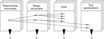
Figure 2: How defects propagate over documents

We see that a requirements defect can lead to several defects in design documents as well as test specifications. The design defects can again propagate to the code and to (glass-box) test specifications. For each document type $k$ we have the set of defects $I_{k}$ and hence the total set of defects $I$ is $I=\bigcup{I_{k}}$. Furthermore, for each defect, we also look at its predecessor defects $R_{i}$. For the model this has the effect that a defect can only be found by a technique if neither the defect itself nor one of its predecessors was detected by an earlier used technique.

3.2 Equations

We give an equation for each of the three components with respect to single defect-detection techniques first and later for a combination of techniques.

3.2.1 Direct Costs

The direct costs are those costs that can be directly measured from the application of a defect-detection technique. They are dependent on the length $t$ of the application. Fig. 3 shows systematically the components of the direct costs.

Figure 3: The components of the direct costs

From this we can derive the following equation containing the three cost types for a technique.

$$d_{A}=u_{A}+e_{A}(t)+\sum_{i}{(1-\theta_{A}(i,t))v_{A}(i)},$$ (1)

where $u_{A}$ are the setup costs, $e_{A}(t)$ the execution costs, and $v_{A}(i)$ the fault removal costs specific to that technique. Hence, we have for a technique its fixed setup costs, execution costs depending on the length of the technique and for each fault in the software removal costs if the technique is able to find it.

3.2.2 Future Costs

In case we were not able to find defects, these will result in costs in the future. We divide these costs into the two parts fault removal costs in the field $v_{F}(i)$ and failure effect costs $f_{F}(i)$. The latter contain all support and compensation costs as well as annoyed customers as far as possible.

$$t_{A}=\sum_{i}{\pi_{i}\theta_{A}(i,t)(v_{F}(i)+f_{F}(i))},$$ (2)

where $\pi_{i}=P$(fault $i$ is activated by randomly selected input and is detected and fixed) [23]. Hence, it describes the probability that the defect leads to a failure in the field.

3.2.3 Revenues

We do not only have costs with defect-detection techniques but also revenues. These revenues are essentially saved future costs. With every fault that we find in-house we avoid higher costs in the future. Therefore, we have the same cost categories but look at the faults that we find instead of the ones we are not able to detect.

$$r_{A}=\sum_{i}{\pi_{i}(1-\theta_{A}(i,t))(v_{F}(i)+f_{F}(i))}$$ (3)

3.2.4 Combination

Typically, more than one technique is used to find defects. The intuition behind that is that they find (partly) different defects. These dependencies are often ignored when the efficiency of defect-detection techniques is analysed. Nevertheless, this has a huge influence on the economics and efficiency. In our view, the notion of diversity of techniques from Littlewood et al. [23] is very useful in this context. The covariance of the difficulty functions of faults describes the similarity of the effectiveness regarding fault finding. We already use the difficulty functions in the present model and therefore are able to express the diversity implicitly.

For the direct costs it means that we sum over all different applications of defect-detection techniques. We define that $X$ is the ordered set of the applied defect-detection techniques. In each application we use Eq. 1 with the extension that we not only take the probability that the technique finds the fault into account but also that the ones before have not detected it. Here also the defect propagation needs to be considered, i.e., that not only the defect itself has not been detected but also its predecessors $R_{i}$.

$$\begin{split}d_{X}=\sum_{x\in X}{\biggl{[}u_{x}+e_{x}(t_{x})}+\sum_{i}{\Bigl{(}(1-\theta_{x}(i,t_{x}))}\\ \phantom{d_{X}=}\prod_{y<x}{\theta_{y}(i,t_{y})}\prod_{j\in R_{i}}{\theta_{y}(j,t_{y})}\Bigr{)}v_{x}(i)\biggr{]}\end{split}$$ (4)

The total future costs are simply the costs of each fault with the probability that it occurs and all techniques failed in detecting it and its predecessors.

$$\begin{split}t_{X}=\sum_{i}{\biggl{[}\pi_{i}\prod_{x\in X}{\theta_{x}(i,t_{x})}}\\ \phantom{t_{X}}\prod_{y<x}{\prod_{j\in R_{i}}{\theta_{y}(j,t_{y})}}(v_{F}(i)+f_{F}(i))\biggr{]}\end{split}$$ (5)

The equation for the revenues uses again a sum over all technique applications. In this case we look at the faults that occur, that are detected by a technique and neither itself nor its predecessors have been detected by the earlier applied techniques.

$$\begin{split}r_{X}=\sum_{x\in X}{\sum_{i}{\biggl{[}\Bigl{(}\pi_{i}(1-\theta_{x}(i,t_{x}))\prod_{y<x}{\theta_{y}(i,t_{y})}}}\\ \prod_{j\in R_{i}}{\theta_{y}(j,t_{y})}\Bigr{)}\bigl{(}v_{F}(i)+f_{F}(i)\bigr{)}\biggr{]}\end{split}$$ (6)

3.2.5 ROI

One interesting metric based on these values is the return on investment (ROI) of the defect-detection techniques. If we look at the total ROI we have to use Eqns. 4, 5, and 6 for the calculation.

$$\mbox{ROI}=\frac{r_{X}-d_{X}-t_{X}}{d_{X}+t_{X}}$$ (7)

This metric is suitable for a single post-evaluation of the quality assurance of a project. However, it alone cannot give an answer whether the effort was cost-optimal.

3.3 Forms of the Difficulty Functions

The notion of difficulty of the defect detection is a very central one in the described model. As mentioned this notion is based on an idea from [23]. However, the original difficulty functions have no concept of time or effort spent but only of one usage or two usages and so on. To be able to analyse and optimise the spent effort for each technique, we need to introduce that additional dimension in the difficulty functions, i.e., the functional form depending on the spent effort. Actually, the equations given for the model above already contain that dimension but it is not further elaborated. This gap is closed in the following.

Firstly, we do not have sufficient data to give an empirically founded basis for the forms of the difficulty functions. Nevertheless, we can formulate hypotheses to identify the most probable distributions for different defects. Secondly, keep in mind that a difficulty function is defined for a specific defect-detection technique detecting a specific defect. That means that each defect can have distinct distribution for each possible technique.

3.3.1 Exponential Function

The function that most obviously models the process under investigation is an exponential function. The intuition is that with more effort spent the difficulty decreases, i.e., the probability of detecting that defect increases. However, with increasing effort the rate of difficulty reduction slows down. The defect detection gets more and more complicated when the “obvious” cases all have been tried.

For this we use a function similar to the density function of an exponential distribution:

$$\theta(i,t)=\left\{\begin{array}[]{ll}\lambda e^{-\lambda t}&\mbox{if $t>0$}\\ 1&\mbox{otherwise}\end{array}\right.,$$ (8)

with $\lambda$ being a parameter that is determined from empirical data from the technique and the defect. It is the inverse of the mean value of the empirically measured difficulty.

3.3.2 Linear and Constant Function

The linear difficulty function models the intuition that there is a steady decrease in difficulty. A review might be an example that employs such a behaviour. The more I read, the higher the possibility that I detect that specific defect. The function can be formulated as follows:

$$\theta_{A}(\tau_{i},t)=mt+1,$$ (9)

where $m$ is the (negative) slope of the straight line.

The constant function constitutes a special case of the linear form of the difficulty functions. In this case the spent effort does not matter because the difficulty of detecting the defect is always the same. The intuitive explanation for this functional form is best explained using the example of a static analysis tool. These tools often use bug patterns specific for a language and thereby identify code sections that are critical. When searching for a specific bug pattern it is of no importance how much effort is spent but if the tool is not able to detect a specific pattern – or only in seldom cases – the probability of detection does not change. We can also use this distribution to model that a specific technique $A$ cannot detect a specific defect $i$ by specifying that $\theta_{A}(i,t)=1$ for all $t$.

3.3.3 Sigmoid Function

For our purposes it is sufficient to see the sigmoid function as a variation of the exponential function. Its graph has an S-like shape and hence one local minimum and one local maximum. In this special case we actually use a complementary sigmoid function to get a turned S.

In contrast to the exponential function, the sigmoid function models the intuition that in the beginning it is hard to detect a specific defect and the difficulty does decrease only slowly. However, when a certain amount of effort is spent, the rate increases and chance of detecting the defect increases significantly until we reach a point of satisfaction – similar to the exponential function – where additional effort does not have a large impact. This distribution is also backed by the so-called S-curve of software testing [16]. That S-curve aims in a slightly different direction but also shows that early in testing only a limited number of failures are revealed, then the detection rate increases until a plateau of satisfaction is reached.

3.4 Discussion

The model so far is not suited for a practical application in a company as the quantities used are not easy to measure. Probably, we are unable to get values for $\theta$ of each fault and defect-detection technique. Also the somehow fixed and distinct order of techniques is not completely realistic as some techniques may be used in parallel or only some parts of the software are analysed. However, in a more theoretical setting we can already use the model for important tasks including sensitivity analysis to identify important input factors.

Another application can be to analyse which techniques influence which parts of the model. For instance, in the automatic derivation of test cases from explicit behaviour models (model-based testing) is a relatively new technique for defect detection. This technique can be analysed and compared with traditional, hand-crafted test techniques based on our model. Two of the factors are obviously affected by model-based testing: (1) the setup costs are considerably higher than in hand-crafted tests because not only the normal test environment has to be set up but also a formal (and preferably executable) behaviour has to be developed. On the contrary, the execution cost per test case is then substantially smaller because the generation can be automated to some extent and the model can be used as an oracle to identify failures. Further influences on factors like the difficulty functions are not that obvious but need to be analysed. This example shows that the model can help to structure the comparison and analysis of defect-detection techniques.

4 Sensitivity Analysis

Every newly proposed mathematical model should be subject to various analyses. Apart from the appropriateness of the model to the modelled reality and the validity of estimates and predictions, the dependence of the output on the input parameters is of interest. The quantification of this dependence is called sensitivity analysis. Local sensitivity analysis usually computes the derivative of the model response with respect to the model input parameters. More generally applicable is global sensitivity analysis that apportions the variation in the output variables to the variation of the input parameters. We base the following description of the global sensitivity analysis we use mainly on [33].

4.1 Settings and Methods

Sensitivity analysis is the study of how the uncertainty in the output of a model can be apportioned to different sources of uncertainty in the model input. Still, what do we gain by that knowledge? There are various questions that can be answered by sensitivity analysis. As pointed out in [32] it is important to specify its purpose beforehand. In our context two settings are of most interest: (1) factors priorisation and (2) factors fixing.

4.1.1 Factors Priorisation

The most important factor is the one that would lead to the greatest reduction in the variance of the output if fixed to its true value. Likewise the second most important factor can be defined and so on. The ideal use for the Setting FP is for the prioritisation of research and this is one of the most common uses of sensitivity analysis in general. Under the hypothesis that all uncertain factors are susceptible to determination, at the same cost per factor, Setting FP allows the identification of the factor that is most deserving of better experimental measurement in order to reduce the target output uncertainty the most. In our context, that means that we can determine the factors that are most rewarding to measure most precisely.

4.1.2 Factors Fixing

This setting is similar to factors priorisation but still has a slightly different flavour. Now, we do not aim to prioritise research in the factors but we want to simplify the model. For this we try to find the factors that can be fixed without reducing the output variance significantly. For our purposes this means that we can fix the input factor at any value in its uncertainty range without changing the outcome significantly.

4.1.3 FAST

There are various available methods for global sensitivity analysis. The Fourier amplitude sensitivity test (FAST) is a commonly used approach that is based on Fourier developments of the output functions. It also allows an ANOVA-like decomposition of the model output variance. In contrast to correlation or regression coefficients, it is not dependent on the goodness of fit of the regression model. The results give a quantification of the influences of the parameters, not only a qualitative ranking as the Morris method, for example.

With the latest developments of this method, it is able not only to compute the first-order effects of each input parameter but also the higher-order and total effects. The first order effect is the influence of a single input parameter on the output variance, whereas the total effects also capture the interaction between input parameters. This is also important for the different settings as the first-order effects are used for the factors priorisation setting, the total-order effects for the factors fixing setting.

4.1.4 SimLab

We use the sensitivity analysis tool SimLab [34] for the analysis. Inside the tool we need to define all needed input parameters and their distributions of their uncertainty ranges. For this, different stochastic distributions are available. The tool then generates the samples needed for the analysis. This sample data is can be read from a file into the model – in our case a Java program – that is expected to write its output into a file with a specified format. This file is read again from SimLab and the first-order and total-order indexes are computed from the output.

4.2 Input Factors and Data

We describe the analysed scenario, factors and data needed for the sensitivity analysis in the following. The distributions are derived from the survey [38, 37]. We base the analysis on an example software with 1000 LOC and with 10–15 faults. The reason for the small number of faults is the increase in complexity of the analysis for higher numbers of faults.

4.2.1 Techniques

We have to base the sensitivity analysis on common or average distributions of the input factors. This also implies that we use a representative set of defect-detection techniques in the analysis. We choose seven commonly used defect-detection techniques and encode them with numbers: requirements inspection (0), design inspection (1), static analysis (2), code inspection (3), (structural) unit test (4), integration test (5), and (functional) system test (6). As indicated we assume that unit testing is a structural (glass-box) technique, system testing is functional (black-box), and integration testing is both. The usage of those seven techniques, however, does not imply that all of them are used in each sample as we allow the effort $t$ to be null.

4.2.2 Additional Factors

To express the defect propagation concept of the model we added the additional factor $\rho$ as the number of predecessors. The factor $c$ represents the the defect class meaning the type of artifact the defect is contained in. This is important for the decision whether a certain technique is capable to find that specific defect at all. The factor $\phi$ encodes the form of difficulty function that is used for a specific fault and a specific technique. We include all the forms presented above in Sec. 3.3. The sequence $s$ of techniques determines the order of execution of the techniques. We allow several different sequences including nonsense orders in which system testing is done first and requirements inspections as the last technique. Finally, the average labour costs per hour $l$ is added because it is not explicitly included in the model equations from Sec. 3.2. Note, that we excluded the effect costs from the sensitivity analysis because we have not sufficient data to give any probability distribution.

4.3 Results and Observations

This section summarises the results of applying the FAST method for sensitivity analysis on the data from the example above and discusses observations. The analysed output factor is the return-on-investment (ROI).

4.3.1 Abstract Grouping

We first take an abstract view on the input factors and group them without analysing the input factors for different techniques separately. Hence, we only have 11 input factors that are ordered with respect to their first and total order indexes in Tab. 1. The first order indexes are shown on the left, the total order indexes on the right.

Table 1: The first and total order indexes of the abstract grouping

$c$	0.4698	$c$	0.8962
$t$	0.1204	$v_{f}$	0.4473
$\bar{\theta}$	0.0699	$\bar{\theta}$	0.4255
$v_{f}$	0.0541	$u$	0.3916
$\phi$	0.0365	$t$	0.3859
$u$	0.0297	$\phi$	0.2888
$v$	0.0264	$\rho$	0.2711
$\rho$	0.0256	$v$	0.2546
$\pi$	0,0158	$\pi$	0,2068
$s$	0,0083	$s$	0,1825
$l$	0,0010	$l$	0,1489

The first order indexes are used for the factors priorisation setting. We see that the types of documents or artifacts the defects are contained in are most rewarding to be investigated in more detail. One reason might be that we use a uniform distribution because we do not have more information on the distribution of defects over document types. However, this seems to be an important information. The factor that ranks second highest is the spent effort. This approves the intuition that the effort has strong effects on the output and hence needs to be optimised. Also the average difficulty of of finding a defect with a technique and the costs of removing a defect in the field are worth to be investigated further. Interestingly, the labour costs, the sequence of technique application, and the failure probability in the field do not contribute strongly to the variance in the output. Hence, these factors should not be the focus in further research.

For the factors fixing setting, the ordering of the input factors is quite similar. Again the failure probability in the field, the sequence of technique application and the labour costs can be fixed without significantly changing the output variance. The factors that definitely cannot be fixed are again the document types, the removal costs in the field, and the average difficulty values. The setup costs rank higher with these indexes and hence should not be fixed.

4.3.2 Detailed Grouping

After the abstract grouping, we form smaller groups and differentiate between the factors with regard to different defect-detection techniques. The first and total order indexes are shown in Tab. 2 again with the first order indexes on the left and the total order indexes on the right.

Table 2: The first and total order indexes of the detailed grouping

$c$	0.2740	$c$	0.7750
$t_{1}$	0.0601	$\phi_{4}$	0.3634
$\pi$	0.0528	$t_{1}$	0.3332
$\phi_{4}$	0.0492	$\pi$	0.3200
$\phi_{1}$	0.0391	$v_{f}$	0.2821
$v_{3}$	0.0313	$v_{3}$	0.2802
$\phi_{0}$	0.0279	$\phi_{1}$	0.2728
$\rho$	0.0278	$\rho$	0.2706
$\phi_{2}$	0.0269	$v_{1}$	0.2574
$v_{f}$	0.0252	$s$	0.2524
$\phi_{6}$	0.0222	$\bar{\theta}_{5}$	0.2493
$v_{0}$	0.0219	$\bar{\theta}_{0}$	0.2312
$\phi_{3}$	0.0216	$\bar{\theta}_{3}$	0.2300
$\bar{\theta}_{6}$	0.0214	$\phi_{6}$	0.2287
$v_{5}$	0.0212	$\phi_{2}$	0.2240
$\bar{\theta}_{0}$	0.0209	$\bar{\theta}_{1}$	0.2077
$s$	0.0208	$v_{5}$	0.2039
$\bar{\theta}_{1}$	0.0203	$\phi_{0}$	0.1966
$v_{1}$	0.0203	$u_{3}$	0.1913
$\bar{\theta}_{4}$	0.0197	$v_{0}$	0.1907
$\phi_{5}$	0.0194	$\bar{\theta}_{6}$	0.1894
$\bar{\theta}_{5}$	0.0186	$\phi_{5}$	0.1892
$t_{2}$	0.0185	$\phi_{3}$	0.1854
$\bar{\theta}_{3}$	0.0181	$v_{4}$	0.1807
$v_{6}$	0.0142	$t_{5}$	0.1719
$v_{2}$	0.0139	$v_{6}$	0.1709
$v_{4}$	0.0120	$\bar{\theta}_{4}$	0.1707
$\bar{\theta}_{2}$	0.0109	$v_{2}$	0.1633
$t_{6}$	0.0089	$t_{6}$	0.1619
$t_{4}$	0.0058	$u_{5}$	0.1451
$t_{3}$	0.0051	$t_{4}$	0.1409
$t_{5}$	0.0034	$u_{4}$	0.1404
$u_{5}$	0.0018	$t_{2}$	0.1378
$u_{0}$	0.0013	$t_{0}$	0.1268
$u_{4}$	0.0010	$l$	0.1222
$t_{0}$	0.0009	$\bar{\theta}_{2}$	0.1125
$u_{3}$	0.0007	$u_{6}$	0.1122
$u_{6}$	0.0007	$u_{0}$	0.1085
$u_{1}$	0.0005	$t_{3}$	0.1053
$u_{2}$	0.0005	$u_{1}$	0.1034
$l$	0.0002	$u_{2}$	0.0996

The main observations from the abstract grouping for the factor priorisation setting are still valid. The type of artifact the defect is contained in still ranks highest and has the most value in reducing the variance. However, in this detailed view, the failure probability in the field ranks higher. This implies that this factor should not be neglected. We also see that for some techniques the form of the difficulty function has a strong influence and that the setup costs of most techniques rank low.

Similar observations can be made for the factors fixing setting and the total order indexes. The main observations are similar as in the abstract grouping. Again, the failure probability in the field ranks higher. Hence, this factor cannot be fixed without changing the output variance significantly. A further observation is that some of the setup costs can be set to fixed value what reduces the measurement effort.

4.4 Discussion and Consequences

From the observations above we can conclude that the labour costs, the sequence of technique application and the removal costs of most techniques are not an important part of the model and the variation in effort does not have strong effects on the output, i.e., the ROI in our case. On the other hand, the type of artifact or document the defect is contained in, the difficulty of defect detection, and the removal costs in the field have the strongest influences.

This has several implications: (1) We need more empirical research on the distribution of defects over different document types and the removal costs of defects in the field to improve the model and confirm the importance of the factor, (2) we still need more empirical studies on the effectiveness of different techniques as this factor can largely reduce the output variance, (3) the labour costs do not have to be determined in detail and it does not seem to be relevant to reduce those costs, (4) further studies on the sequence and the removal costs are not necessary.

5 Practical Application

As we discussed above, the theoretical model can be used for analyses but is too detailed for a practical application. The main goal is, however, to optimise the usage of defect-detection techniques which requires a applicability in practice. Hence, we need to simplify the model to reduce the needed quantities.

5.1 General

For the simplification of the model, we use the following additional assumptions:

• Faults can be categorised in useful defect types.

• Defect types have specific distributions regarding their detection difficulty, removal costs, and failure probability.

• The linear functional form of the difficulty approximates all other functional forms sufficiently.

We define $\tau_{i}$ to be the defect type of fault $i$. It is determined using the defect type distribution of older projects. In this way we do not have to look at individual faults but analyse and measure defect types for which the determination of the quantities is significantly easier. In the practical model we assumed that the defects can be grouped in “useful” classes or defect types. For reformulating the equation it was sufficient to consider the affiliation of a defect to a type but for using the model in practice we need to further elaborate on the nature of defect types and how to measure them.

For our economics model we consider the defect classification approaches from IBM [16] and HP [9] as most suitable because they are proven to be usable in real projects and have a categorisation that is coarse-grained enough to make sensible statements about each category.

We also lose the concept of defect propagation as it was shown not to have a high priority in the analyses above but it introduces significant complexity to the model. Hence, the practical model can be simplified notably.

5.2 Equations

Similar to Sec. 3.2 where we defined the basic equations of the ideal model, we formulate the equations for the practical model using the assumptions from above.

5.2.1 Single Economics

We start with the direct costs of a defect-detection technique. Now we do not consider the ideal quantities but use average values for the cost factors. We denote this with a bar over the cost name.

$$d_{A}=\bar{u}_{A}+\bar{e}_{A}(t)+\sum_{i}{(1-\theta_{A}(\tau_{i},t))\bar{v}_{A}(\tau_{i})},$$ (10)

where $\bar{u}_{A}$ is the average setup cost for technique $A$, $\bar{e}_{A}(t)$ is the average execution cost for $A$ with length $t$, and $\bar{v}_{A}(\tau_{i})$ is the average removal cost in defect type $\tau_{i}$. Apart from using average values, the main difference is that we consider defect types in the difficulty functions. The same applies to the revenues.

$$r_{A}=\sum_{i}{\pi_{\tau_{i}}(1-\theta_{A}(\tau_{i},t))(\bar{v}_{F}(\tau_{i})+\bar{f}_{F}(\tau_{i}))},$$ (11)

where $\bar{f}_{F}(\tau_{i})$ is the average effect costs of a fault of type $\tau_{i}$. Finally, the future costs can be formulated accordingly.

$$t_{A}=\sum_{i}{\pi_{\tau_{i}}\theta_{A}(\tau_{i},t)(\bar{v}_{F}(\tau_{i})+\bar{f}_{F}(\tau_{i}))}.$$ (12)

With the additional assumptions, we can also formulate a unique form of the difficulty functions:

$$\theta_{A}(\tau_{i},t_{a})=mt_{A}+1,$$ (13)

where $m$ is the (negative) slope of the straight line. If a technique is not able to detect a certain type, we will set $m=0$.

5.2.2 Combined Economics

Similarly, the extension to more than one technique can be done.

$$\begin{split}d_{X}=\sum_{x\in X}{\biggl{[}\bar{u}_{x}+\bar{e}_{x}(t_{x})}+\sum_{i}{(1-\theta_{x}(\tau_{i},t_{x}))}\\ \prod_{y<x}{\Bigl{(}\theta_{y}(\tau_{i},t_{y})}\Bigr{)}\bar{v}_{x}(\tau_{i})\biggr{]}\end{split}$$ (14)

$$t_{X}=\sum_{i}{\pi_{\tau_{i}}\prod_{x\in X}{\Bigl{(}\theta_{x}(\tau_{i},t_{x})\Bigr{)}\Bigl{(}\bar{v}_{F}(\tau_{i})+\bar{f}_{F}(\tau_{i})\Bigr{)}}}$$ (15)

$$\begin{split}r_{X}=\sum_{x\in X}{\sum_{i}{\pi_{\tau_{i}}(1-\theta_{x}(\tau_{i},t_{x}))}}\\ \prod_{y<x}{\Bigl{(}\theta_{y}(\tau_{i},t_{y})}\Bigr{)}\Bigl{(}\bar{v}_{F}(\tau_{i})+\bar{f}_{F}(\tau_{i})\Bigr{)}\end{split}$$ (16)

5.3 Sensitivity Analysis

Similar to the analyses in Sec. 4 we determined the first and total order indexes of the practical model again with data from [38, 37]. The results are shown in Tab. 3 with the first order indexes left and the total order indexes right. We have to note that we only looked at defects in the code because we have no empirical data on defect types in other kinds of documents. Furthermore, we introduced the factor $\alpha$ that denotes the fraction of defects of a specific defect type.

Table 3: The first and total order indexes from the practical model

$t$	0.1196	$t$	0.8855
$\pi$	0.1138	$v_{f}$	0.8670
$\bar{\theta}$	0.1097	$s$	0.7881
$\alpha$	0.0975	$\bar{\theta}$	0.7857
$v_{f}$	0.0694	$l$	0.7772
$l$	0.0634	$\alpha$	0.6676
$s$	0.0592	$\pi$	0.6200
$u$	0.0476	$u$	0.4902
$v$	0.0018	$v$	0.0958

We see that the effort for the techniques ranks highest in both settings. The failure probability again ranks high in the factors priorisation setting. Hence, this factor should be investigated in more detail. Similarly to the ideal model, the setup and removal costs of the techniques do not contribute strongly to the output variance.

In the factors fixing setting, we see that the setup and removal costs can be fixed without changing the variance significantly. This implies that we can use coarse-grained values here. Also the failure probability can be taken from literature values. More emphasis, however, should be put on the effort, the removal costs in the field, and the sequence of technique application. Of which the last one is surprising as for the ideal model this factor ranked rather low.

5.4 Optimisation

For the optimisation only two of the three components of the model are important because the future costs and the revenues are dependent on each other. There is a specific number of faults that have associated costs when they occur in the field. These costs are divided in the two parts that are associated with the revenues and the future costs, respectively. The total always stays the same, only the size of the parts varies depending on the used defect-detection techniques. Therefore, we use only the direct costs and the revenues for optimisation and consider the future costs to be dependent on the revenues.

Therefore, the optimisation problem can be stated by: maximise $r_{X}-d_{X}$. By using Eq. 14 and Eq. 16 we get the following equation to be maximised.

$$\begin{split}\sum_{x}{\biggl{[}-\bar{u}_{x}-\bar{e}_{x}(t_{x})+\sum_{i}{(1-\theta_{x}(\tau_{i},t_{x}))}}\\ \prod_{y<x}{(\theta_{y}(\tau_{j},t_{y}))}\bigl{(}\pi_{\tau_{i}}\bar{v}_{F}(\tau_{i})+\pi_{\tau_{i}}\bar{f}_{F}(\tau_{i})-\bar{v}_{x}(\tau_{i})\bigr{)}\biggr{]}\end{split}$$ (17)

The equation shows in a very concise way the important factors in the economics of defect-detection techniques. For each technique there is the fixed setup cost and the execution costs that depend on the effort. Then for each fault in the software (and over all fault classes) we use the probability that the technique is able to find the fault and no other technique has found the fault before to calculate the expected values of the other costs. The revenues are the removal costs and effect costs in the field with respect to the failure probability because they only are relevant if the fault leads to a failure. Finally we have to subtract the removal costs for the fault with that technique which is typically much smaller than in the field.

For the optimisation purposes, we probably also have some restrictions, for example a maximum effort $t_{\textit{max}}$ with $\sum_{x}{t_{x}}\leq t_{\textit{max}}$, either fixed length or none $t_{A}=\{0,100\}$, or some fixed orderings of techniques, that have to be taken into account. The latter is typically true for different forms of testing as system tests are always later in the development than unit tests.

Having defined the optimisation problem and the specific restrictions we can use standard algorithms for solving it. It is a hard problem because it involves multi-dimensional optimisation over a permutation space, i.e., not only the length of technique usage can be varied but also the sequence of the defect-detection techniques.

5.5 Applications

In this section, we describe two possibilities how the practical model can be used.

We can use the model in experiments as well as during normal software development. As discussed in Sec. 3.4 we can use the ideal model to explain the effects of techniques on the economics. The practical model is suited to measure important aspects of defect-detection techniques in software engineering experiments by finding difficulty functions of certain techniques in certain domains. In software projects, the practical model can also help to optimise the future quality assurance by using the information from old projects.

5.5.1 In-House

The main idea is to predict the future economics based on the data from finished projects. The approach should then contain the following parts:

• Classify found faults

• Which technique found which fault?

• Which faults were found in the field?

• Estimate failure probability and costs for each fault

From this data, we can estimate the needed quantities. This estimation process can have different forms. The failure probability can either be estimated by expert opinion or using field data if it was a field failure. The cost data can be partly taken from effort measurements during development and from the field. Then we can try to answer the two questions: What is the optimal length of a technique and what is the optimal combination? However, not that the results are in all cases dependent on the problem class and domain because they have a huge influence on the costs.

5.5.2 Domain-Specific

A second application could be to try to generalise the results of the model to a complete domain either from field studies or experiments. There are probably specific defect types in specific domains for which we might be able to collect data that is not only valid inside one company but for the whole domain. In this way, data from other companies could be used for optimisation purposes.

6 Related Work

Our own previous work on the quality economics of defect-detection techniques forms the basis of this model. We formulated some simple relationships of cost factors and how this could be used in evaluating and comparing different techniques in [36]. This is refined in [40] and additional means to predict future costs are incorporated. Some first results of the current model and sensitivity analysis can be found in [39].

The available related work can generally classified in two categories: (1) theoretical models of the effectiveness and efficiency of either test techniques or inspections and (2) economic-oriented, abstract models for quality assurance in general. The first type of models is able to incorporate interesting technical details but are typically restricted to a specific type of techniques and often economical considerations are not taken into account. The second type of models typically comes from more management-oriented researchers that consider economic constraints and are able to analyse different types of defect-detection but often contain the technical details in a very abstract way.

Pham describes in [30] various flavours of a software cost model for the purpose of deciding when to stop testing. It is a representative of models that are based on reliability models. The main problem with such models is that they are only able to analyse system testing and no other defect-detection techniques and the differences of different test techniques cannot be considered.

Holzmann describes in [10] his understanding of the economics of software verification. He describes some trends and hypotheses that are similar to ours and we can support most ideas although they need empirical justification at first.

Kusumoto et al. describe in [22, 21] a metric for cost effectiveness mainly aimed at software reviews. They introduce the concept of virtual software test costs that denote the testing cost that have been needed if no reviews were done. This implies that we always want a certain level of quality.

A model similar to the Kusomoto model but with an additional concept of defect propagation was proposed by Freimut et al. in [6].

The economics of the inspection process are investigated in [1]. This work also uses defect classes and severity classes to determine the specific costs. However, it identifies only the smaller removal costs to be the benefit of an inspection.

An example of theoretical models of software testing is the work of Morasca and Serra-Capizzano [25]. They concentrate on the technical details such as the different failure rates. In this paper there is also a detailed review of similar models.

Ntafos describes some considerations on the cost of software failure in [27]. The difficulties of collecting appropriate data are shown but the model itself is described only on an abstract level.

In [20, 35] a metric called return on software quality (ROSQ) is defined. It is intended to financially justify investments in quality improvement. The underpinnings of this metric are similar to the analytical model defined in this paper although there are significant differences. Firstly, it aims mainly on measuring the effects of process improvements, i. e. constructive quality assurance, whereas we concentrate on analytical quality assurance. Secondly, they base the calculations mainly on average defect content in the software and do not consider the important question if the faults lead to failures.

In [18] the model of software quality costs is set into relation to the Capability Maturity Model (CMM) [29]. The emphasis is hence on the prevention costs and how the improvement in terms of CMM levels helps in preventing failures.

Galin extends in [8, 7] the software quality costs with managerial aspects but the extensions are not relevant in the context of defect-detection techniques.

Guidelines for applying a quality cost model in a business environment in general are given in [17]. Mandeville describes in [24] also software quality costs, a general methodology for cost collection, and how specific data from these costs can be used in communication with management.

Humphrey presents in [12] his understanding of software quality economics. The defined cost metrics do not represent monetary values but only fractions of the total development time. Furthermore, the effort for testing is classified as failure cost instead of appraisal cost.

Collofello and Woodfield propose in [4] a metric for the cost efficiency but do not incorporate failure probabilities or difficulties.

Based on the general model for software cost estimation COCOMO, the COQUALMO model was specifically developed for quality costs in [3]. This model is different in that it is aiming at estimating the costs beforehand and that it uses only coarse-grained categories of defect-detection techniques. In our work, we want to analyse the differences between techniques in more detail.

Boehm et al. also present in [2] the iDAVE model that uses COCOMO II and COQUALMO. This model allows a thorough analysis of the ROI of dependability. The main difference is again the granularity. Only an average cost saving per defect is considered. We believe that analysing costs per defect type can improve estimates and predictions.

Building on iDAVE, Huang and Boehm propose a value-based approach for determining how much quality assurance is enough in [11]. In some respect that work is also more coarse-grained than our work because it considers only the defect levels from COQUALMO. However, it contains an interesting component that deals with time to market costs that are currently missing from our model.

A somehow similar model to COQUALMO in terms of the description of the defect introduction and removal process is described in [13]. However, it offers means to optimise the resource allocation. The only measure for defect-detection techniques used is defect removal efficiency.

7 Conclusions

We finally summarise our work and the main contributions and give some directions for future work.

7.1 Summary

We propose an analytical model of quality economics with a strong focus on defect-detection techniques. This focus is necessary to be able to be more detailed than comparable approaches. In this way, we incorporate different cost types that are essential for evaluating defect-detection techniques and also a notion of reliability or the probability of failure. The latter is also very important because it is significant which faults are found in terms of reliability. This distinguishes the model from more abstract approaches. On the other hand we have models derived from software reliability modelling. These models are typically simpler but can only be used on techniques where reliability models can be applied, i. e. mainly system tests. We aim to incorporate all types of defect-detection techniques.

One of the main contributions is also the research priorisation. We find that it is most rewarding to further investigate the distribution of defect over document types, the removal costs in the field, and the difficulty, especially the functional form with respect to varying effort. All of these have not been subject to extensive empirical work.

The main weakness of our model is that the ideal model is not usable in real software projects. Hence, we derived a practical model that is based on defect types. This gives us a greater data basis for each type. The problem here is, that it is not totally clear if this structuring in defect types really is able to give useful distributions of the removal costs, removal difficulty, and failure probability. Furthermore, it strongly depends on how “good” these types are defined and we currently have no requirements on the classes.

7.2 Future Work

As future work, we consider working on support for the estimation of the needed quantities of the practical model, especially the number of faults $\bar{I}$ and also on the probability of failure of the defects as those are important factors. An application of the model to a real project and thereby analysing the predictive validity of the model is one of next major steps.

The optimisation must be worked on in more detail and effective tool support is essential to make the model applicable in practice. Finally, an incorporation of time to market might be beneficial because there are important costs associated with time overruns that need to be considered. In some markets this may be even more important than all the other factors contained in the model.

8 Acknowledgments

We are grateful to Sandro Morasca for detailed comments on the model and to Bev Littlewood for helping on the understanding of their diversity model. This research was supported by the Deutsche Forschungsgemeinschaft (DFG) within the project InTime.

References

- [1] S. Biffl. Hierarchical Economic Planning of the Inspection Process. In Proc. Third International Workshop on Economics-Driven Software Engineering Research (EDSER-3). IEEE Computer Society Press, 2001.
- [2] B. Boehm, L. Huang, A. Jain, and R. Madachy. The ROI of Software Dependability: The iDAVE Model. IEEE Software, 21(3):54–61, 2004.
- [3] S. Chulani and B. Boehm. Modeling Software Defect Introduction and Removal: COQUALMO (COnstructive QUALity MOdel). Technical Report USC-CSE-99-510, University of Southern California, Center for Software Engineering, 1999.
- [4] J. S. Collofello and S. N. Woodfield. Evaluating the Effectiveness of Reliability-Assurance Techniques. Journal of Systems and Software, 9(3):191–195, 1989.
- [5] A. V. Feigenbaum. Total Quality Control. McGraw-Hill, 4rd edition, 2005.
- [6] B. Freimut, L. C. Briand, and F. Vollei. Determining Inspection Cost-Effectiveness by Combining Project Data and Expert Opinion. IEEE Transactions on Software Engineering, 31(12):1074–1092, 2005.
- [7] D. Galin. Software Quality Assurance. Pearson, 2004.
- [8] D. Galin. Toward an Inclusive Model for the Costs of Software Quality. Software Quality Professional, 6(4):25–31, 2004.
- [9] R. B. Grady. Practical Software Metrics for Project Management and Process Improvement. Prentice-Hall, 1992.
- [10] G. J. Holzmann. Economics of Software Verification. In Proc. 2001 ACM SIGPLAN–SIGSOFT Workshop on Program Analysis for Software Tools and Engineering (PASTE’01), pages 80–89. ACM Press, 2001.
- [11] L. Huang and B. Boehm. Determining How Much Software Assurance is Enough? A Value-based Approach. In Proc. Seventh Workshop on Economics-Driven Software Research (EDSER-7), 2005.
- [12] W. S. Humphrey. A Discipline for Software Engineering. The SEI Series in Software Engineering. Addison-Wesley, 1995.
- [13] P. Jalote and B. Vishal. Optimal Resource Allocation for the Quality Control Process. In Proc. 14th International Symposium on Software Reliability Engineering (ISSRE’03), 2003.
- [14] C. Jones. Applied Software Measurement: Assuring Productivity and Quality. McGraw-Hill, 1991.
- [15] J. M. Juran and A. B. Godfrey. Juran’s Quality Handbook. McGraw-Hill Professional, 5th edition, 1998.
- [16] S. H. Kan. Metrics and Models in Software Quality Engineering. Addison-Wesley, 2nd edition, 2002.
- [17] C. Kaner. Quality Cost Analysis: Benefits and Risks. Software QA, 3(1):23–27, 1996.
- [18] S. T. Knox. Modeling the costs of software quality. Digital Technical Journal, 5(4):9–16, 1993.
- [19] H. Krasner. Using the Cost of Quality Approach for Software. CrossTalk. The Journal of Defense Software Engineering, 11(11):6–11, 1998.
- [20] M. S. Krishnan. Cost and Quality Considerations in Software Product Management. PhD thesis, Carnegie Mellon University, 1996.
- [21] S. Kusumoto. Quantitative Evaluation of Software Reviews and Testing Processes. PhD dissertation, Osaka University, 1993.
- [22] S. Kusumoto, K. ichi Matasumoto, T. Kikuno, and K. Torii. A New Metric for Cost Effectiveness of Software Reviews. IEICE Transactions on Information and Systems, E75-D(5):674–680, 1992.
- [23] B. Littlewood, P. T. Popov, L. Strigini, and N. Shryane. Modeling the Effects of Combining Diverse Software Fault Detection Techniques. IEEE Transactions on Software Engineering, 26(12):1157–1167, 2000.
- [24] W. A. Mandeville. Software Costs of Quality. IEEE Journal on Selected Areas in Communications, 8(2):315–318, 1990.
- [25] S. Morasca and S. Serra-Capizzano. On the Analytical Comparison of Testing Techniques. In Proc. 2004 ACM SIGSOFT International Symposium on Software Testing and Analysis (ISSTA ’04), pages 154–164. ACM Press, 2004.
- [26] G. J. Myers. The Art of Software Testing. John Wiley & Sons, 1979.
- [27] S. C. Ntafos. The Cost of Software Failures. In Proc. IASTED Software Engineering Conference, pages 53–57. IASTED/ACTA Press, 1998.
- [28] S. C. Ntafos. On Comparisons of Random, Partition, and Proportional Partition Testing. IEEE Transactions on Software Engineering, 27(10):949–960, 2001.
- [29] M. C. Paulk, C. V. Weber, B. Curtis, and M. B. Chrissis. The Capability Maturity Model: Guidelines for Improving the Software Process. The SEI Series in Software Engineering. Addison Wesley Professional, 1995.
- [30] H. Pham. Software Reliability. Springer, 2000.
- [31] A. Rai, H. Song, and M. Troutt. Software Quality Assurance: An Analytical Survey and Research Prioritization. Journal of Systems and Software, 40:67–83, 1998.
- [32] A. Saltelli. Global Sensitivity Analysis: An Introduction. In Proc. 4th International Conference on Sensitivity Analysis of Model Output (SAMO ’04), pages 27–43. Los Alamos National Laboratory, 2004.
- [33] A. Saltelli, S. Tarantola, F. Campolongo, and M. Ratto. Sensitivity Analysis in Practice – A Guide to Assessing Scientific Models. John Wiley & Sons, 2004.
- [34] SimLab 2.2. http://webfarm.jrc.cec.eu.int/uasa/primer/index.asp, 2005.
- [35] S. A. Slaughter, D. E. Harter, and M. S. Krishnan. Evaluating the Cost of Software Quality. Communications of the ACM, 41(8):67–73, 1998.
- [36] S. Wagner. Towards Software Quality Economics for Defect-Detection Techniques. In Proc. 29th Annual IEEE/NASA Software Engineering Workshop (SEW-29), pages 265–274. IEEE Computer Society, 2005.
- [37] S. Wagner. A Literature Survey of the Software Quality Economics of Defect-Detection Techniques. In Proc. 5th ACM-IEEE International Symposium on Empirical Software Engineering (ISESE ’06). ACM Press, 2006.
- [38] S. Wagner. A Literature Survey of the Software Quality Economics of Defect-Detection Techniques. Technical report, Institut für Informatik, Technische Universität München, 2006.
- [39] S. Wagner. Modelling the Quality Economics of Defect-Detection Techniques. In Proc. 4th Workshop on Software Quality (4-WoSQ). ACM Press, 2006.
- [40] S. Wagner and T. Seifert. Software Quality Economics for Defect-Detection Techniques Using Failure Prediction. In Proc. 3rd Workshop on Software Quality (3-WoSQ), pages 11–16. ACM Press, 2005.