Depth-Based Visual Servoing Using Low-Accurate Arm

Abstract

This paper proposes a visual-servoing method dedicated to grasping of daily-life objects. In order to obtain an affordable solution, we use a low-accurate robotic arm. Our method corrects errors by using an RGB-D sensor. It is based on SURF invariant features which allows us to perform object recognition at a high frame rate. We define regions of interest based on depth segmentation, and we use them to speed-up the recognition and to improve reliability. The system has been tested on a real-world scenario. In spite of the lack of accuracy of all the components and the uncontrolled environment, it grasps objects successfully on more than 95% of the trials.

I Introduction

Visual servoing refers to robot control based on visual information. Computer vision is used to analyze the visual data acquired by the robots. The data are provided by one or several cameras, which can be placed directly on the robot manipulator (eye-in-hand), on a mobile robot or somewhere fixed in the workspace. Grasping objects with a robot in a daily environment is a complex task that service robots have to perform. The grasping problem refers to choosing an optimal final state for the manipulator and the forces to apply with its fingers.

The focus of this article is about the robustness of visual servoing based on depth information toward a low-accurate robotic arm. In particular, the choice of the final state of the gripper is simplified by considering only cylindrical objects and grasping them perpendicularly to the revolution axis of the cylinder.

In this paper, we present an entire grasping system. In contrast to the system used in [1], our goal is to grasp an object used in the daily life such as a bottle. While our method can be extended to support other situations, we make the following assumptions in our experiments: the object is mostly cylindrical, its size is known and the background is not dark. The system is designed to be embedded on service robots. Therefore, the sensor is placed above the basis of the arm, on the same mobile platform. Since affordability is a crucial point when designing service robots, the system has been tested with a low-accurate robotic arm. While in article such as [2] and [3] simulation or industrial robots are used to test the algorithms, these methods of evaluation do not fit the purpose of this paper.

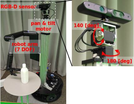
Figure 1: The robot used for the experiments

The experiments of this system were performed using a 7 DOF (Degrees Of Freedom) robotic arm, the iARM manufactured by Exact Dynamics. This robotic arm is designed to be used by disabled people who control it using their own vision to move it to a target position. Therefore, it was designed to be controlled by a vision-based control loop and not only with a target position. When controlled in position, it presents an accuracy of about 3 cm. It is important to note that the error has a low repeatability, and therefore it is not possible to learn a deterministic model for the error. The RGB-D sensor used was an Asus Xtion PRO LIVE and its orientation was controlled by servomotors from Dynamixel. Figure 1 shows the robot used and the possible moves of the pan-tilt. In this paper, the model of the robot is constructed based on the distances between its different parts such as the arm basis, the camera and the servomotors.

Visual servoing using eye-in-hand cameras has been proven very successful [4, 5, 6, 7, 8] even on moving targets. However, most robotic arms come with no vision system, and the integration of an eye-in-hand camera is problematic, especially if the arm has to go through narrow spaces or if there is a collision risk. Moreover, cable of the camera being disconnected was responsible for 13 failures out of 198 grasping trials in [8]. In our approach, we use a camera installed on a pan-tilt mount in order to avoid such problems. While we propose a tracking approach based on identifying the fingers of the grippers, other alternatives based on depth images exist such as [9], in which neither pose estimation nor feature extraction are required.

The main information used by our algorithm is noisy depth measurement results provided by the RGB-D sensor. Our approach does not aim toward optimal control, but toward real-time control. Actually, it has been proven in [10] that optimal control is difficult in presence of noise in the depth measurement. Moreover, optimal control is suited for industrial environments while this paper focuses on service robots. We use the color information to extract and match SURF features [11] while in [4], SIFT features [12] are used. The architecture of a mobile manipulator using SURF features to estimate the pose of objects is presented in [13]. We use depth-based segmentation to obtain different regions of interest, thus allowing us to run the local features matching on a subset. This allows us to reduce the computation time and improve the accuracy of the position estimation [14].

We measure the robustness of the system against errors in the model by artificially adding errors in it. According to the results provided in [10], it shows that real-time control is an appropriate solution.

This paper makes four contributions:

1. An algorithm to detect regions of interest in depth images provided by RGB-D sensor.

2. A solution to keep a high frame rate while using a large set of SURF features [11] for object recognition in real time.

3. A method of real-time tracking of the gripper based on regions of interest.

4. An experiment showing the accuracy improvement when visual servoing is used.

The reliability of the proposed system has been confirmed by experimental results, as well as its robustness against errors in the model. Therefore, the designed system gives satisfying results, even when using low-accurate robotic arms.

This paper is organized as follows: Section II discusses the related work in the areas of vision-based grasping and object recognition. The detection method of regions of interest for object detection is proposed in Section III. The probabilistic database of references is presented in Section IV. In Section V, we discuss the filter proposed to estimate the position of the object. Section VI describes the system proposed to track the position of the gripper in real-time. The experimental scenario and an overview of the results are presented in Section VII. Finally, a conclusion is given in Section VIII.

(a) Image (chosen column highlighted in red)

(b) Depth

(c) Depth 1^st derivate

(d) Depth 2^nd derivative

Figure 2: Example of derivatives estimations for a column of an image

II Related research for object recognition

Object recognition paradigm has radically evolved since the apparition of the SIFT algorithm [12]. While object recognition was previously based on template matching, it is now essentially based on invariant features. However extracting and matching SIFT features was time consuming. Several new types of features have been proposed by the computer vision community. The SURF algorithm [11] outperforms SIFT in both quality and time consumption. The use of binary descriptors has been brought by BRISK [15]. Although it is less robust to changes of factors, it needs dramatically less computational resources than SURF. A fast approximation method for the matching problem has been developed as a part of the library presented in [16]. Finding a homography from the set of matches is usually done by using RANSAC [17]. Reducing the area of the image to a region of interest containing the object improves the quality of the results and decrease the computation time [14].

A real-time plane segmentation using RGB-D sensors is detailed in [18]. Although it detects only plane objects, it presents an interest for image segmentation since the computed information could be used in addition to color information to improve color-based segmentation. A scene interpreter based only on depth information is described in [19]. It uses an accurate depth sensor and does not indicate the computation time required but it shows a very high accuracy.

Different approaches to the grasping problem have been proposed in the robotics community. In [2], objects are divided into three categories: known (model of the object is available), familiar (previous experience over similar objects are available) and unknown (there is no knowledge about the object available). The problem of using previous grasping experience to increase the success rate is discussed in [2]. A method for the grasping of unknown objects is presented in [3]. Reaching the grasping point by using a visual based control loop is discussed in [1], this article uses markers on the gripper to compute its orientation more easily. The arm we use has an accuracy of about 3 cm. This is presumably much less accurate than the robotic arms used in [2] and [3].

III Detecting regions of interest

The system starts by detecting regions of interest (ROI) based on the depth image captured by the RGB-D sensor. The advantage of using a depth-based sensor over a stereo-camera is that it allows to detect objects independently of their color difference from the background.

To perform efficient segmentation, two different kinds of edges need to be detected.

• Sudden changes in depth, when the object hides a farther background. It corresponds to a local peak in the first derivative.

• Changes of surface orientation, when there is no noticeable difference of depth between the object and the plane on which it is lying.

The differences between these two kinds of edges can be observed in Fig. 2. Units used are $mm$ for millimeters and $p$ for pixel. The image used is shown in Fig. 2(a). The column of the image which is used as an example is colored in red. The corresponding depth acquired by the sensor is shown in Fig. 2(b).

Edges are detected both horizontally and vertically, using approximations of the first and second derivative of the depth image. The kernels used for derivation are $K_{h}$ and $K_{v}$ as defined in Eq. (1) and Eq. (2). The effects of the values $k_{1}$ and $k_{2}$ are shown in Fig. 2(c) and Fig. 2(d). The values $k_{1}$ and $k_{2}$ are used as $k$ for the first and the second derivations respectively. Kernels of an odd length and height are used in order to apply them with a centered anchor. This helps to avoid shift in edge detection.

$$K_{h}(k)=[-1,0_{1\times 2k-1},1]$$ (1)

$$K_{v}(k)=[-1,0_{1\times 2k-1},1]^{T}$$ (2)

Using a threshold on the absolute value of the first derivative allows us to detect sudden depth changes as can be seen in Fig. 2(c) at row 40. However, the same process does not work for the second derivative. In order to detect the edge around row 150 in Fig. 2(d), the threshold required would be low enough to detect a very thick edge around the sudden depth changes as in row 40. A mask is used for detecting the second derivative in order to avoid detecting edges which have already been detected by the threshold on the first derivative. This mask is obtained by performing a dilatation (a well-known morphological process) on the edges already detected. In order to reduce the number of remaining edges, an erosion process is performed once the threshold has been applied.

Using the depth image shown in Fig. 3(a), horizontal and vertical edges are detected using the first and second derivative. By gathering them, we obtain the image shown in Fig. 3(b). A dilatation is then performed in order to ensure that the contours of the object are connected as shown in Fig. 3(c). A set of superpixels is obtained by applying a floodfill algorithm as shown in Fig. 3(d) (Floodfill algorithm from the computer vision library OpenCV is used). A first filter based on the size of the superpixel is applied to the set of superpixels obtained by applying the floodfill algorithm in order to remove the background and noise. Then, by using the depth information and the position of the pixels, the superpixels properties (i.e the height and the width of the superpixel) are computed. The obtained properties for each superpixel are compared with the expected properties. If it does not match, then the superpixel is discarded. The remaining superpixels (shown in Fig. 3(e)) are the ROI obtained from the depth image. Those regions are highlighted in red in the corresponding color image as shown in Fig. 3(f).

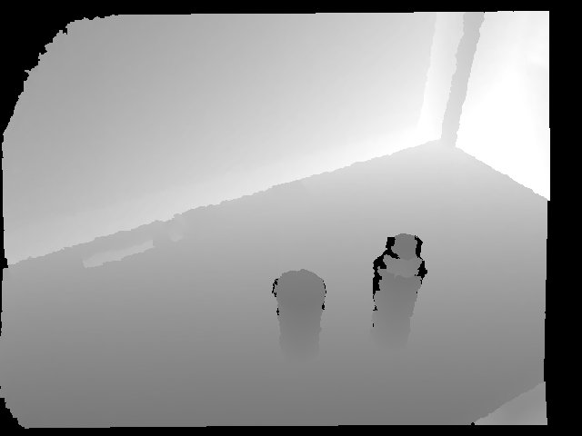
(a) Depth image

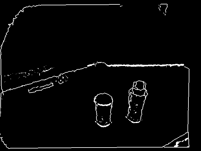
(b) Detected contours

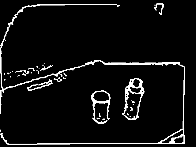
(c) Contours after dilatation

(d) Superpixels

(e) Filtered Superpixels

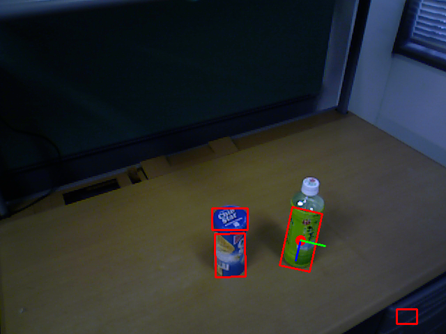
(f) Detected ROI

Figure 3: Depth segmentation in six images

IV Probabilistic database of references

In our system, each reference consists of a set of SURF features computed in a ROI obtained through the process described above. A large number of references are used for every object in order to compensate for the small number of features detected due to the size of the ROI. The database of references stores all the references corresponding to an object. The main goal of making this database is to allow the use of a large number of references while keeping a low computation time in order to ensure real-time processing.

Once the set of ROI has been computed, each of the regions has to be compared with the references by matching features of the references and those of the input image. Using all the references for each frame would lead to a low frame rate, which is inversely proportional to the number of references in the database. In order to ensure that the frame rate does not depend on the number of references, we only use a random subset of the references with a bounded maximal size. In order to increase progressively the chances to obtain a match, two rules are applied. For each reference of the subset, if at least one of the ROI matches it, then we increase the probability of selecting. On the other side, if none of the ROI matches the reference, we decrease the probability of selecting it.

Let $n$ be the number of references of the database, ${R=\left(r_{1},\dots,r_{n}\right)}$ be a set of references of the database and ${W=\left(w_{r_{1}},\dots,w_{r_{n}}\right)}$ be a set of weights for the references. Then, three properties are ensured by the database:

• The probability of obtaining reference $r$ is directly influenced by its weight $w_{r}$.

• $\sum\limits_{w\in W}w=1$.

• Let $m$ and $M$ be the minimal and the maximal weights chosen by the user respectively. Then ${\forall w\in W,m\leq w\leq M}$. Ensuring this property avoids issues due to floating point approximation when the weight of a reference would be approximated by 1 or 0. It also allows to keep a non-zero probability of obtaining each reference.

An example of picking references from the database is shown in Fig. 4. Every reference is chosen at most once, even if two random numbers point to the same reference. Therefore, when five references are requested, a subset containing four references might be selected (e.g. in Fig. 4). While this might be considered as a drawback of this algorithm, it turns out to be an advantage, because the average number of references in the random subset is reduced when the weight of a reference is significantly higher than $\frac{1}{n}$. Such a situation happens only if this reference has been successfully matched with one of the ROI. By reducing the number of references of the subset in this situation, the required processing time highly decreases while the probability for matching only slightly decreases.

The corrected weight for reference $z_{r}$ is computed by using (3) if matching has been successful and (4) if it has not. If the reference did not belong to the picked subset, then $z_{r}=w_{r}$. Two different gains are defined, $G_{s}$ and $G_{f}$. When a match has been found, $G_{s}$ is used. If no matches have been found, $G_{f}$ is used. Both gains have to be positive and smaller than 1. These gains represent the learning rates. Typical values used in experiments are $G_{s}=0.3$ and $G_{f}=0.04$.

$$z_{r}=w_{r}+G_{s}(M-w_{r})$$ (3)

$$z_{r}=w_{r}-G_{f}(w_{r}-m)$$ (4)

After these updates, the sum of all $z_{r}$ might be different from 1. We end up the update by normalization which depends on ${\delta=1-\sum\limits_{r\in R}z_{r}}$.

Let us define $u_{r}=M-w_{r}$ as the weight which can be added to a reference before reaching the maximal value and $v_{r}=w_{r}-m$ as the weight which can be removed of a reference before reaching the minimal value. Let us define $U=\sum\limits_{r\in R}u_{r}$ and $V=\sum\limits_{r\in R}v_{r}$ as the total weights which can be added and removed from the references before reaching global saturation, respectively. Define $w^{\prime}_{r}$ as the final weight of a reference after normalization. If $\delta>0$, then it is computed according to Eq. (5), else it is computed according to Eq. (6).

$$w^{\prime}_{r}=z_{r}+\frac{u_{r}}{U}\delta$$ (5)

$$w^{\prime}_{r}=z_{r}+\frac{v_{r}}{V}\delta$$ (6)

Figure 4: Picking randomly five elements out of the eight references from the database

V Filtering the object position

Even if the object to grasp is not supposed to move quickly, it is important to use multiple detection results for determining the object position. This can lower the false positive rate and improve the accuracy of the position estimation at the same time. Since the object detection part has a non-zero probability of confusing objects, it is necessary to remove the detected positions which do not fit with the other results. This is achieved by remembering the last $l$ successful results of the object detection and removing the $j$ results which bring the highest error, where $l$ and $j$ are two positive integers. The results of the object detection are provided with an index of confidence based on the number of matched features, it provides an estimate of the quality of the matching. In order to increase the impact of recent information, a timestamp is associated with each result.

Each entry of the filter is composed of four different elements:

• computed position of the object; $h$

• quality of the detection (index of confidence); $q$

• associated timestamp; $t$

• detected axis of the object; $a$

The state of filter $F$ is described formally by the following equation:

$$\begin{array}[]{lcl}F&=&\{e_{1},\dots,e_{l}\}\\ &=&\left\{(h_{1},q_{1},t_{1},a_{1}),\dots,(h_{l},q_{l},t_{l},a_{l})\right\}\end{array}$$ (7)

Let $b_{i}$ be the weight of the entry $(h_{i},q_{i},t_{i},a_{i})$ at time $T$. Then, the weight is calculated as follows:

$$b_{i}=\frac{q_{i}}{T-t_{i}}$$ (8)

Therefore, it is easy to see that the weight of an entry is proportional to its quality and inversely proportional to the elapsed time since this entry appeared.

Let $E(F)$ be the object position estimated from the state of the filter, and it is computed accordingly to Eq. (9).

$$E(F)=\frac{\sum\limits_{i=1}^{l}{h_{i}b_{i}}}{\sum\limits_{i=1}^{l}{b_{i}}}$$ (9)

Let $Q(F)$ be the detection quality obtained from the state of the filter and $\alpha$ be a constant used as a gain. Then, $Q(F)$ is computed accordingly to Eq. (10).

$$Q(F)=\frac{\sum\limits_{i=1}^{l}\lVert E(F)-h_{i}\rVert b_{i}}{\sum\limits_{i=1}^{l}{b_{i}}}\times\frac{\sum\limits_{i=1}^{l}\frac{1}{T-t_{i}}}{\alpha}$$ (10)

In order to remove eventual false positives, we rank all the entries $e_{i}$ according to the value $Q(F\setminus e_{i})$, where $F\setminus e_{i}$ represents $F$ without the $i$-th component $e_{i}$. Then, we build a new set $F^{\prime}=\{e^{\prime}_{1},\dots,e^{\prime}_{l-j}\}$ by removing from $F$ the $j$ entries which led to the lowest value. Thus, the final filter value and quality are represented by $E(F^{\prime})$ and $Q(F^{\prime})$, respectively. It is important to note that $F^{\prime}$ needs to be updated when a new entry is added.

VI Tracking the gripper position

Gripper tracking is necessary to correct the mechanical errors when using low-accurate robotic arms. However, it is still possible to use the estimation of the position according to the arm controller to improve the efficiency of tracking. We chose to detect both fingers of the gripper separately.

First, we use the data provided by the arm controller to compute the bounding boxes which are supposed to contain the fingers. Then, we increase the size of both bounding boxes by taking into account the maximal error of the arm $\epsilon$. The obtained spaces $E_{1}$ and $E_{2}$ are described in Eq. (11). The projection of those spaces on an image is shown in Fig. 5.

$$\begin{split}E_{i}=\left\{{{}^{G}(x,y,z)}\left|\!\!\begin{array}[]{l}x\in[\frac{s_{i}g_{w}-f_{w}}{2}-\epsilon,\frac{s_{i}g_{w}+f_{w}}{2}+\epsilon]\\ y\in[\frac{-f_{t}}{2}-\epsilon,\frac{f_{t}}{2}+\epsilon]\\ z\in[-f_{l}-\epsilon,\epsilon]\\ \end{array}\!\!\!\!\right.\right\}\\ \parbox[l]{173.44534pt}{ \vspace{0.5cm} Where:\\ ${}^{G}(x,y,z)$ a point in the gripper basis\\ $g_{w}$ the width of the gripper\\ $f_{w}$ the width of a finger\\ $f_{t}$ the thickness of a finger\\ $f_{l}$ the length of the finger\\ $\epsilon$ the maximal error accepted\\ $s_{i}$ the side of the object: $s_{1}=-1$ and $s_{2}=1$ }\end{split}$$ (11)

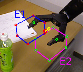
Figure 5: Projections of the possible arm finger positions on an image

Once the spaces $E_{1}$ and $E_{2}$ have been computed, it is possible to use the basis transformation to project them on the images from the RGB-D sensor. The projection of $E_{1}$ and $E_{2}$ on the camera image is a polygon. Let $x_{m}$ and $y_{m}$ be the minimal $x$ and $y$ of the polygon respectively, and $x_{M}$ and $y_{M}$ be the maximal $x$ and $y$ of the polygon respectively. Then the regions of interest are defined by the rectangles which have the four following corners: $(x_{m},y_{m})$, $(x_{M},y_{m})$, $(x_{M},y_{M})$ and $(x_{m},y_{M})$. Only these regions of the image are selected and both the projections and the spaces $E_{1}$ and $E_{2}$ are used later in the gripper detection process.

The previous step allows us to compute a region of interest that should contain the finger. Then two main steps are still requested to obtain the visual position of the finger. Segmentation of the gripper needs to be performed and the position of the finger has to be computed from the segmentation result.

In order to remove the pixels which do not belong to the space, we check for every pixel if it belongs to the space. However, since this requires to compute a basis transform for every pixel, two steps are performed before it. First points which do not belong to the projection are removed as shown in Fig. 6(a). Then, color information are used to remove pixels from the background as shown in Fig. 6(b). In our case, only black pixels are considered. Once all the conditions with a low computational cost have been checked, the remaining pixels belonging to the spaces $E_{1}$ and $E_{2}$ are checked. If it is not possible to differentiate the background from the gripper by using color information, the process is slowed because pixels belonging to space has to be checked for more pixels.

A debugging image allowing to understand the space checking process is shown in Fig. 6(c). Here, the blue, green and red components of the image are respectively set to the maximal values if the point matches the ${}^{G}x$, ${}^{G}y$ and ${}^{G}z$ ranges defined in Eq. (11) (e.g. Pixels matching the range ${}^{G}x$ and ${}^{G}z$ but not ${}^{G}y$ are colored in purple which is the addition of blue and red). Only the pixels colored in white are retained in the filtered image shown in Fig. 6(d).

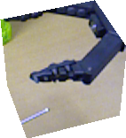
(a) Projection of the space on the image

(b) Color matching pixels

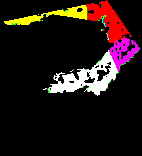
(c) Space check

(d) Filtered ROI

Figure 6: Filtering a region of interest

The image shown in Fig. 6(d) is a binary one. This allows us to run a floodfill algorithm to obtain a set of superpixels. Finally, only the largest superpixel is retained, removing the noise which might have passed the previous filtering steps. If the obtained superpixel is large enough, the position of the finger is calculated as the average of the remaining pixels. If there is no large enough superpixel, the finger is considered as undetected.

A Kalman filter is used to estimate the final position of the gripper. It uses a single position which is computed by using the results of the finger detections. Since fingers can be undetected, it is necessary to handle different cases.

• Both fingers detections fail: In this case, it is not possible to compute the gripper position from the image. A detection failure result is given to the Kalman filter.

• One finger detection succeeds Let $\beta_{t}$ be the theoretical distance from the finger detected to the gripper. By assuming that the orientation error of the gripper is small, it is possible to estimate the visual position of the gripper $g_{v}$ by using the visual position of the finger $f_{v}$. The resulting value $g_{v}$ is given to the Kalman filter.

  $$g_{v}\approx f_{v}+\beta_{t}$$ (12)

• The two fingers are detected: The estimated position of the finger is the average of the positions of the two fingers. If the distance between the two fingers positions matches the expected distance, this value is given to the Kalman filter. If the difference between the visual distance of the two fingers and the theoretical distance is too large, a detection failure is given to the Kalman filter instead.

When a failure detection is sent to the Kalman filter, the values of the associated covariance matrix are increased, increasing the uncertainty about the gripper position and speed. While the uncertainty is below a given threshold, the camera focus on the estimated position and a correction is applied to the requested position using a simple proportional action. If the uncertainty is too high, then the gripper stops and waits for the filter to stabilize.

VII Experimental results

We conducted the experiments about the robustness of our grasping system by running a set of trials. The database used for these experiments contained 50 RGB-D images for each of the five objects used and was built by moving objects inside the grasping area. While several objects were presented in the database, only one was used for the experiments. Closing the gripper to grasp the object was achieved by requesting an finger space slightly lower than the diameter of the object. All the trials were made on a laptop using a windows operating system, the processor used was an Intel i3-2310M (2.1 GHz, Dual-core). We used the C++ implementation of OpenCV 2.4.

The task designed to evaluate the performance was as follows: the object was placed alone on a table, the robotic arm was always starting at the same position, gripper initially opened. When the grasping task was launched, the reference database for visual detection was loaded, and the score of all the references were set as equivalent in order to avoid influence from the previous detections, the only input from the user side was the name of the object which needs to be grasped. The evaluation task was to detect the object, grasp it and lift it 15 cm above the original position. Neither the orientation of the object nor its position with respect to the robot were fixed. However, the object was placed inside a circle with a diameter of 20 cm. We assumed six possible results for a grasping task: four failures and two successes.

Object not detected:

After 30 s, if the object has not been detected by the vision module, then the object detection is considered as a failure and the trial is stopped.

Gripper lost:

If the gripper detection system cannot manage to track the gripper, the system will not be able to bring the gripper to destination in less than 30 s. In this case, the gripper is considered as lost and the trial is stopped.

Grasping failed:

On the way to the destination, the gripper might collide with another object. The gripper might also close while it is not on the object. In both cases, the grasping part is considered as a failure.

Lifting failed:

Sometimes, the gripper closes on the object but not accurately enough to lift it and the object falls while trying to lift it. In this case, the lifting is considered as a failure.

Object touched:

If the object has been lifted with success but there was a contact between the gripper and the object before the gripper started to close, then the trial is considered as a partial success.

Object not touched:

If the object has been lifted with success and there was no contact between the gripper and the object before closing the gripper, then the trial is considered as a success.

Distinction between failures allows to know which part of the system is the weakest, and distinction between successes allows us to estimate the accuracy of the system.

Two different approaches were compared:

Non-Visually Guided Grasping (NVGG):

Tracking of the gripper is not activated and the estimate of the gripper position is directly given by the controller of the robotic arm.

Visually Guided Grasping (VGG):

This method uses the detection system described previously to estimate the gripper position.

Both use the object recognition system proposed in this article.

It is shown in TABLE I that without injected error, both methods succeeded to lift the object in more than 95% of the trials. The main advantage of using VGG is that the rate of success without touching the object before closing the gripper is significantly higher. The frequency of Object not touched is 70% when using VGG, while it is only 54% when using NVGG.

This difference of accuracy is highlighted with the results of another experiment where errors were introduced in the distance between the arm and the camera. The error vector which was added to the model had a length of 4 cm, and was computed randomly at the beginning of each trial. The results are shown in TABLE II and it illustrates that when the model of the robot is not accurate, VGG strongly outperforms NVGG. The frequency of Success is 72% when using VGG while it is only 48% when using NVGG. Moreover, the frequency of Object not touched is 54% when using VGG, while it is only 12% when using NVGG.

The time needed to converge to an accurate estimate of the position of the object was also recorded and is shown in Fig. 7. This measure represents the time required before the quality of the filter grows above the hand-tuned threshold, which ensures that the estimation of the object position is reliable. In more than 60% of the cases, the time needed to detect the object and to estimate its position was within 2 s. It was greater than 4 s in less than 10% of the cases. However, there are still isolated cases when the detection takes more than 20 s. This is due to the fact that the set of references did not cover all the possible cases. Sometimes the matching between the current state of the object and the references was hard to establish because there was not sufficient references.

The matching time for each frame using the probabilistic database proposed here was compared to the required time per frame when using all references in Fig. 8. The proposed method allows to use only a subset of references, ensuring that the matching time is not proportional to the number of references. The data were computed from 20 different videos of 10 s and only the convergence time was examined.

TABLE I: Grasping results by method

	Result	Count	Frequency
NVGG	Success	50	100%
	Object not touched	21	42%
	Object touched	29	57%
VGG	Success	49	98%
	Object not touched	35	70%
	Object touched	14	28%
	Failure	1	2%
	Object not detected	1	2%

TABLE II: Grasping results by method with 40 mm error in the model

	Result	Count	Frequency
NVGG	Success	24	48%
	Object not touched	6	12%
	Object touched	18	36%
	Failure	26	52%
	Object not detected	3	6%
	Grasping failed	11	22%
	Lifting failed	12	24%
VGG	Success	36	72%
	Object not touched	27	54%
	Object touched	9	18%
	Failure	14	28%
	Gripper lost	7	14%
	Grasping failed	3	6%
	Lifting failed	4	8%

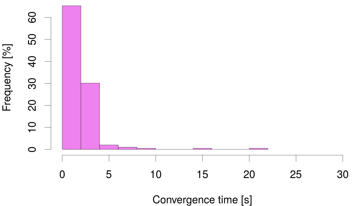
Figure 7: Histogram of convergence time

Figure 8: Matching time by method

VIII Conclusion

We presented an entire grasping system which shows a high success rate even when the position of the gripper given by the model is not accurate. In contrast to other approaches with high performances, our system offers a possibility of using very low-accurate robotic arms. Since the cost of service robots is a crucial issue, we believe that the proposed system is a major step toward their globalization.

Amongst the further research into this system, we aim to improve the database of references in order to develop the ability of learning new objects autonomously. Another step which needs to be taken in order to provide a grasping system adapted to daily life environment is collision avoidance when planning the gripper trajectory.

References

- [1] R. Horaud, F. Dornaika, and B. Espiau, “Visually guided object grasping,” IEEE Trans. Robotics and Automation, vol. 14, no. 4, pp. 525–532, 1998.
- [2] J. Bohg and D. Kragic, “Grasping familiar objects using shape context,” in Int. Conf. on Advanced Robotics (ICAR), 2009.
- [3] G. Kootstra, M. Popovic, J. A. Jørgensen, K. Kuklinski, K. Miatliuk, D. Kragic, and N. Krüger, “Enabling grasping of unknown objects through a synergistic use of edge and surface information,” Int. Journal of Robotic Research, vol. 31, no. 10, pp. 1190–1213, 2012.
- [4] A. Maxim, C. Lazar, A. Burlacu, and C. Copot, “Robotic visual servoing system based on SIFT features,” in 16th Int. Conf. on System Theory, Control and Computing (ICSTCC), oct 2012, pp. 1–6.
- [5] F. Chaumette and S. Hutchinson, “Visual servo control. I. Basic approaches,” IEEE Robotics Automation Magazine, vol. 13, no. 4, pp. 82–90, 2006.
- [6] W. Hong and J. Slotine, “Experiments in Hand-Eye Coordination Using Active Vision,” in Fourth International Symposium on Experimental Robotics (ISER), 1995.
- [7] G. Recatala, P. J. Sanz, E. Cervera, and A. P. Del Pobil, “Grasp-based visual servoing for gripper-to-object positioning,” in Proc. IEEE/RSJ Int. Conf. on Intelligent Robots and Systems (IROS 2004), vol. 1, sep 2004, pp. 118–123 vol.1.
- [8] K. M. Tsui, A. Behal, D. Kontak, and H. A. Yanco, “I want that: Human-in-the-loop control of a wheelchair-mounted robotic arm,” Applied Bionics and Biomechanics, vol. 8, no. 1, pp. 127–147, 2011.
- [9] C. Teulière and E. Marchand, “A Dense and Direct Approach to Visual Servoing Using Depth Maps,” IEEE Trans. Robotics, vol. 30, no. 5, pp. 1242–1249, oct 2014.
- [10] E. Malis, Y. Mezouar, and P. Rives, “Robustness of Image-Based Visual Servoing With a Calibrated Camera in the Presence of Uncertainties in the Three-Dimensional Structure,” IEEE Trans. Robotics, vol. 26, no. 1, pp. 112–120, 2010.
- [11] H. Bay, A. Ess, T. Tuytelaars, and L. Van Gool, “Speeded-Up Robust Features (SURF),” Computer Vision and Image Understanding, vol. 110, no. 3, pp. 346–359, 2008.
- [12] D. G. Lowe, “Object recognition from local scale-invariant features,” in Proc. Seventh IEEE Int. Conf. on Computer Vision (ICCV), vol. 2, 1999, pp. 1150–1157 vol.2.
- [13] K. T. Song and C. H. Chang, “Object pose estimation for grasping based on robust center point detection,” in Control Conference (ASCC), 2011 8th Asian, 2011, pp. 305–310.
- [14] L. T. Anh and J. B. Song, “Robotic grasping based on efficient tracking and visual servoing using local feature descriptors,” International Journal of Precision Engineering and Manufacturing, vol. 13, no. 3, pp. 387–393, 2012.
- [15] S. Leutenegger, M. Chli, and R. Y. Siegwart, “BRISK: Binary Robust invariant scalable keypoints,” in Proceedings of the IEEE International Conference on Computer Vision, 2011, pp. 2548–2555.
- [16] M. Muja and D. Lowe, “Scalable Nearest Neighbour Algorithms for High Dimensional Data,” IEEE Trans. Pattern Analysis and Machine Intelligence, vol. PP, no. 99, p. 1, 2014.
- [17] M. A. Fischler and R. C. Bolles, “Random Sample Consensus: A Paradigm for Model Fitting with Applications to Image Analysis and Automated Cartography,” Communications of the ACM, vol. 24, no. 6, pp. 381–395, 1981.
- [18] D. Holz, R. Schnabel, D. Droeschel, J. Stückler, and S. Behnke, “Towards semantic scene analysis with time-of-flight cameras,” in Lecture Notes in Computer Science, vol. 6556 LNAI, 2011, pp. 121–132.
- [19] R. B. Rusu, N. Blodow, Z. C. Marton, and M. Beetz, “Close-range Scene Segmentation and Reconstruction of 3D Point Cloud Maps for Mobile Manipulation in Domestic Environments,” in Proc. IEEE/RSJ Int. Conf. on Intelligent Robots and Systems (IROS), 2009, pp. 1–6.