Thermodynamics of a time dependent and dissipative oval billiard: a heat transfer and billiard approach

Abstract

We study some statistical properties for the behavior of the average squared velocity – hence the temperature – for an ensemble of classical particles moving in a billiard whose boundary is time dependent. We assume the collisions of the particles with the boundary of the billiard are inelastic leading the average squared velocity to reach a steady state dynamics for large enough time. The description of the stationary state is made by using two different approaches: (i) heat transfer motivated by the Fourier law and; (ii) billiard dynamics using either numerical simulations and theoretical description.

I Introduction

The initial mark in the investigation of billiards theory is related to Birkhoff ref1 in beginning of last century. Since then this research area has developed significantly. Birkoff considered the investigation of the motion of a free point-like particle – representing a billiard ball – in a bounded manifold. However the modern investigations of billiards are indeed related to the results of Sinai ref3 ; ref3a and Bunimovich ref4 ; add1 who made rigorous demonstrations on the topic.

A billiard is a dynamical system composed of a particle, or an ensemble of non interacting particles, moving confined to a domain with a piecewise-smooth boundary ref5 where they collide. The specular reflections occur under the condition the boundary is sufficiently smooth. In such case the tangent component of the velocity of the particle measured with respect to the border where collision happened is unchanged while the normal component reverses sign. There are many results nowadays considering either static ref6 ; ref7 ; ref8 ; ref8a ; ref8b ; ref8c ; ref8d ; ref8e ; ref8f and time dependent boundaries td2 ; td3 ; ref5a ; ref5b . A phenomenon well known in time dependent boundary is the Fermi acceleration ref9 as well as the so called Loskutov-Ryabov-Akinshin (LRA) conjecture ref10 ; ref11 . Fermi acceleration ref9 is a phenomenon where an ensemble of particles acquires unlimited energy from collisions with an infinitely heavy and moving wall. The conjecture itself claims that if chaos is present in the dynamics of a particle in a static version of the billiard, then this is a sufficient – but not necessary – condition to observe Fermi acceleration when a time perturbation to the boundary is introduced. Many different billiards exhibit Fermi acceleration under time perturbation to the boundary including the Lorentz gas ref12 ; ref12a , oval billiard ref13 , stadium ref14 and other shapes ref17 . The elliptical billiard is an exception and the LRA conjecture does not apply to it. For the static boundary, the elliptical billiard is integrable ref5 and the phase space is composed of rotating and librating orbits. A curve which separates these two different regimes is called as separatrix. Lenz et al. ref19 ; ref20 shown that when the boundary of the billiard is allowed to be time dependent, the separatix curve is replaced by a stochastic layer allowing cross visitations from regions of libration and rotation. For the static case both energy, $E$, and angular momenta about the two foci, $F$, are constants of motion ref21 , leading the system to be integrable. However, when time perturbation is introduced, the observable $F$ (see Ref. ref19 ) experiences strong and fast variations from the crossing of orbits coming from rotation and those leaving from libration. The successive crossings produce the stochasticity required in the LRA conjecture, hence leading the time dependent elliptical billiard to exhibit Fermi acceleration. This result is considered a counter example of the LRA conjecture. Latter on, investigations on different models have proved the Fermi acceleration is not a robust phenomenon since a very small amount of dissipation is enough to suppress the phenomenon ref22 . Consideration of inelastic collisions in the elliptical billiard ref23 has proved the successive crossings of orbits coming from rotation region and entering libration domain – and vice versa – are interrupted suppressing the Fermi acceleration.

The motion of the time dependent boundary can be related to a more physical situation. Due to the thermal fluctuations the position of each atom that compose the boundary is allowed to move locally. Such oscillation of the atoms, and hence of the boundary, can be brought to the context of billiard which allows connections of the observables obtained from the velocity of the particle – hence the kinetic energy – to the thermodynamics, particularly the temperature and entropy.

In this paper we investigate some dynamical properties for an ensemble of particles confined in an oval billiard whose boundary is moving in time. Our main goal is to understand and describe the dynamics of the average squared velocity for a gas of noninteracting particles. We will do this by using two different procedures. Because the boundary of the billiard is moving, as soon as the particles collide, there is a change of energy of the particle. Therefore, the first procedure considered involves the heat transfer Fourier equation. We write and solve the Fourier equation considering the geometrical properties of the boundary. The resulting equation is that the temperature of the gas settles down for sufficiently long time as the temperature of the boundary, hence the average squared velocity, reaches the thermal equilibrium. The second one involves the formalism commonly used in billiard problems. We write down the equations of the mapping that describe the dynamics of the problem and extract some average properties for the squared velocity of the particles. The properties are obtained either by straightforward numerical simulations as well as analytically. The results obtained on the analytical approach are remarkable well fitted by the numerical simulations. The first approach however uses the time as the dynamical variable while the second one uses the number of collisions of the particles with the boundary. The two dynamical variables are not trivially connected among themselves. Therefore, by the use of an empirical function, we find a straight relation between these two parameters.

This paper is organized as follows. In Sec. II we discuss the properties of the average squared velocity by the use of heat transfer Fourier equation. We use some geometrical properties of the boundary to fit into the required parameters of the equation. Section III is devoted to construct the billiards approach of the problem. We them obtain the equations that describe the dynamics of the model and discuss the several types of characterization including steady state, dynamical regime, numerical simulations, critical exponents and the behavior of the probability distribution function for the velocity of the particles. The connection of the two parts is made in Sec. IV where a relation between the time and number of collisions is obtained. Conclusions and discussions are made in Sec. V.

II Heat transfer approach

We discuss in this section the approach involving heat transfer. To start with we assume that there is a set of identical particles moving inside a closed boundary. The density of the particles is considered sufficiently small such that the particles are noninteracting. Figure 1(a) shows an illustration of the system. We assume the boundary of the billiard is moving in time, therefore, this is the mechanism responsible for the exchange of energy with the particles: collisions!

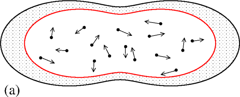
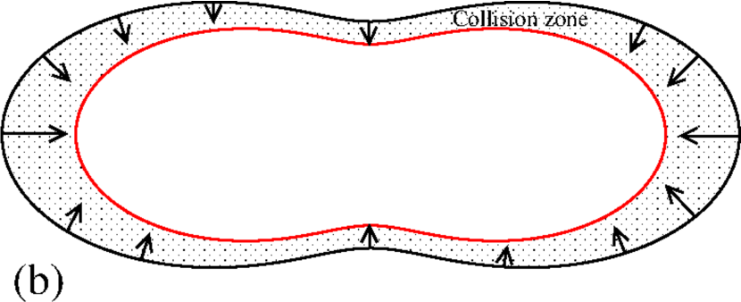
Figure 1: (a) Sketch of the billiard boundary and an ensemble of noninteracting particles. (b) Illustration of the heat transfer region. The arrows direction point the heat flux.

The boundary is at a temperature $T_{b}$ that is considered fixed and does not change with the dynamics of the particles. Hence the boundary works as a thermal bath and two obvious conclusions can be extracted. If the temperature of the gas of particles is less than $T_{b}$, then the boundary gives energy to the particles raising up the temperature of the gas. On the other hand, if the temperature of the particles is larger than $T_{b}$, the heat bath absorbs energy from the particles and dissipate it along with the chain of nearby atoms of the boundary – hence reducing the temperature of the gas. There is a region near the border of the billiard where the particles can exchange energy which we denote as a collision region.

The Hamiltonian that describes the dynamics of each particle is given by

$$H={{p^{2}}\over{2m}}+V(q_{x},q_{y},t),$$ (1)

where $p^{2}=p_{x}^{2}+p_{y}^{2}$ corresponds to the momentum of the particle and $V$ is the potential energy which is written as

$$V(q_{x},q_{y},t)=\left\{\begin{array}[]{ll}0~{}~{}{\rm if}~{}~{}(q_{x},q_{y},t)<R(t)\\ \infty~{}~{}{\rm if}~{}~{}(q_{x},q_{y},t)=R(t)\\ \end{array}\right.,$$ (2)

where $R$ is the radius of the boundary written in polar coordinates, which assumes the following form in this work $R(\theta,\eta,t)=1+\eta f(t)\cos(p\theta)$, where $p$ is any integer number. A non integer number leads to an open boundary to where the particles can escape. $\eta$ is a parameter which controls the circle perturbation. If $\eta=0$, the boundary is a circle, that is integrable ref5 , in billiards terminology, due to the conservation of energy and angular momentum, while $\eta\neq 0$ leads the phase space to be mixed when $f(t)$ is a constant ref21 . The function $f(t)$ leads to the time perturbation of the boundary and we consider in this work two different types of perturbation: (i) periodic oscillations and; (ii) random oscillations. For case (i) the function is written as $f(t)=1+\varepsilon\cos(\omega t)$ where $\varepsilon$ is the amplitude of oscillation and $\omega$ is the angular frequency, which we set it as fixed $\omega=1$. For the random case (ii), the function $f(t)$ assumes the same expression as in the case (i) however, at the instant of the impact, we assume there is a random phase $Z(t)$, given random numbers $Z\in[0,2\pi]$, such that the velocity of the moving boundary is given by $\vec{V}_{b}(t)={{d}\over{dt}}[\vec{R}_{b}(t)+Z(t)]$. This choice is made in such a way to avoid the possibility of having the chance of the particles moving outside of the boundary, hence a non physical situation. At the same time, this is an easy way to introduce randomness in the model. In this section we discuss the thermodynamical properties based on the heat transfer equation – Fourier law – and the geometrical parameters of the boundary will be used in the approach. In next section we describe the dynamics by using the billiards formalism hence writing the dynamical equations of the particle and averaging the velocity as a function of the number of collisions as well as along an ensemble of particles.

The equation that governs the heat transference blu is written as

$${{\partial Q}\over{\partial t}}=-\kappa\ell{{\partial T}\over{\partial x}},$$ (3)

where $\kappa$ corresponds to the heat conductivity coefficient, $\ell$ is length along the boundary to where the heat can flow and is obtained from the geometrical properties of the boundary, ${{\partial Q}\over{\partial t}}$ denotes the flux of heat from a region where there is a temperature difference $\Delta T$ and ${{\partial T}\over{\partial x}}$ corresponds to the temperature gradient. We present a short discussion of the Fourier equation in Appendix 1 and an interpretation of the heat conductivity coefficient $\kappa$ for the one-dimensional case. The minus $(-)$ is related to the fact the heat flow from the region of higher to the lower temperature, hence opposite to the temperature gradient blu . Figure 1(b) illustrates schematically the collision zone and the region to where heat can flow. The effective length $\ell$ to where heat can flow is obtained from $\ell=\int_{0}^{2\pi}R(\theta,\eta,\varepsilon,p,t)d\theta=\int_{0}^{2\pi}[1+\eta[1+\varepsilon\cos(t)]\cos(p\theta)]d\theta=2\pi$.

The two steps we consider to solve Eq. (3) is to obtain the corresponding expressions for: (i) ${{\partial Q}\over{\partial t}}$ and; (ii) ${{\partial T}\over{\partial x}}$ in such a way that its solution can be obtained. We know that the density of particles is considered sufficiently small so that each particle does not interact with any other. Therefore, the energy of each particle is due to the energy associated to the state of its motion, hence kinetic energy. From the energy equipartition theorem we have that

$${{1}\over{2}}m\overline{V^{2}}(t)=KT(t),$$ (4)

where $K$ is the Boltzmann constant and $\overline{V^{2}}(t)$ corresponds to the squared average velocity averaged over the ensemble of particles. The knowledge of $\overline{V^{2}}(t)$ directly gives the temperature $T(t)$.

We know from the thermodynamics blu that an amount of heat transferred in a process depends on the temperature $dQ=cdT$, where $dQ$ is an infinitesimal amount of heat transferred at the price of an infinitesimal variation $dT$ in the temperature. The parameter $c$ corresponds to the heat capacity of the gas of particles. For an ideal gas $c=KN_{p}$ where $N_{p}$ is the total number of particles in the gas loskutov . With these we have the left hand side of Eq. (3) is written as ${{\partial Q}\over{\partial t}}={{cm}\over{2K}}{{\partial}\over{\partial t}}\overline{V^{2}}(t)$. The next step is to obtain the expression of the right side of Eq. (3). Since the temperature gradient can only happen along the collision zone, we can consider an approximation that

$${{\partial T}\over{\partial x}}\cong{{\Delta T}\over{\Delta x}}={{T-T_{b}}\over{\Delta x}},$$ (5)

where $\Delta x$ is measured along the collision zone. To obtain $\Delta x$ we note that the radius of the boundary can assume two extrema: $R_{max}=1+\eta(1+\varepsilon)\cos(p\theta)$ and $R_{min}=1+\eta(1-\varepsilon)\cos(p\theta)$, where $R_{max}$ and $R_{min}$ correspond to the maximum and minimum values of the radius when time varies. The collision zone then is a region given by $\Delta R=R_{max}-R_{min}=2\eta\varepsilon\cos(p\theta)$. We see that $\Delta R$ is not constant being dependent directly on $\theta$ and has the property that $\overline{\Delta R}=0$. Therefore, an approximation for $\Delta x$ is obtained from $\Delta x=\sqrt{\overline{(\Delta R)^{2}}}$ where

$$\overline{(\Delta R)^{2}}={{1}\over{2\pi}}\int_{0}^{2\pi}4\eta^{2}\varepsilon^{2}\cos^{2}(p\theta)d\theta.$$ (6)

A straightforward calculation gives $\Delta x=\sqrt{2}\eta\varepsilon$. Hence the expression of ${{\Delta T}\over{\Delta x}}={{T-T_{b}}\over{\sqrt{2}\eta\varepsilon}}$. Incorporating these approximations in the heat transfer equation we end up with

$${{cm}\over{2K}}{{\partial}\over{\partial t}}{\overline{V^{2}}}=-{{\kappa\ell}\over{\sqrt{2}\eta\varepsilon}}\left[{{m}\over{2K}}{\overline{V^{2}}}-T_{b}\right].$$ (7)

Equation (7) is a first order differential equation and that when solved properly leads to the following result

$$\overline{V^{2}}(t)={{2K}\over{m}}T_{b}+\left[V_{0}^{2}-{{2K}\over{m}}T_{b}\right]e^{-{{2\pi\kappa}\over{\sqrt{2}\eta\epsilon c}}t}.$$ (8)

From the energy equipartition theorem, the temperature is written as

$$T(t)=T_{b}+\left[T_{0}-T_{b}\right]e^{-{{2\pi\kappa}\over{\sqrt{2}\eta\epsilon c}}t}.$$ (9)

Let us now discuss some possibilities to study from experimental approach. Suppose a gas of particles is injected in the billiard with a low initial velocity such that $T_{0}\gg T_{b}$. From Eq. (9) and considering only the dominant term we have

$$T(t)\cong T_{b}+T_{0}e^{-{{2\pi\kappa}\over{\sqrt{2}\eta\epsilon c}}t},$$ (10)

therefore, confirming an exponential decay for short $t$ and a convergence to the stationary state at $T(t)=T_{b}$ when $t\rightarrow\infty$. Other type of behavior is observed when an ensemble of particles is injected in the billiard with very low energy such that $T_{0}\ll T_{b}$. Expanding the exponential in Taylor series and keeping only the dominant term we end up with

$$T(t)=T_{b}{{{2\pi\kappa}\over{\sqrt{2}\eta\epsilon c}}t}.$$ (11)

This result confirms the temperature grows at short time linearly in time hence leading the average velocity $\overline{V}(t)=\sqrt{\overline{V^{2}}}$ to grow with square root of time, hence

$$\overline{V}(t)=\sqrt{T_{b}{{{4\pi K\kappa}\over{\sqrt{2}m\eta\epsilon c}}}}\sqrt{t}.$$ (12)

III Billiards approach

We now discuss how to construct the equations of the mapping that describe the dynamics of the particle inside of the billiard. The mapping gives the angular position of the particle $\theta$, the angle that the trajectory of the particle forms with a tangent line at the position of the collision $\alpha$, the absolute velocity of the particle $|\vec{V}|$ and finally the instant of the collision with the boundary $t$ at the impact $n^{th}$ with the further impact $(n+1)^{th}$. Figure 2 shows a typical illustration of a billiard and the angles used to describe the dynamics of the model.

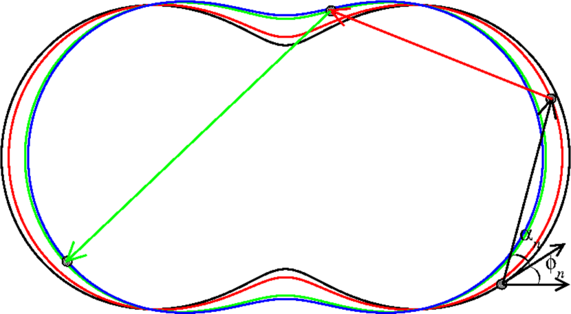
Figure 2: Illustration of four snapshots of the boundary at the four collisions.

The position of the particle at a given state $(\theta_{n},\alpha_{n},|\vec{V}_{n}|,t_{n})$, written as a function of time is

$$X(t) = X(\theta_{n},t_{n})+|\vec{V_{n}}|\cos(\alpha_{n}+\phi_{n})(t-t_{n}),$$ (13)

$$Y(t) = Y(\theta_{n},t_{n})+|\vec{V_{n}}|\sin(\alpha_{n}+\phi_{n})(t-t_{n}),$$ (14)

where the time $t\geq t_{n}$ with $X(\theta_{n},t_{n})=R(\theta_{n},t_{n})\cos(\theta_{n})$ and $Y(\theta_{n},t_{n})=R(\theta_{n},t_{n})\sin(\theta_{n})$. As soon as the $\theta$ is known, the angle $\phi$, which corresponds to the angle between the tangent line and the horizontal at $X(\theta),Y(\theta)$ is $\phi=\arctan[Y^{\prime}(\theta,t)/X^{\prime}(\theta,t)]$ where $Y^{\prime}(\theta,t)=dY/d\theta$ and $X^{\prime}(\theta,t)=dX/d\theta$.

Considering the particle travels with a constant speed between collisions, the distance traveled by the particle measured with respect to the origin of the coordinate system is given by $R_{p}(t)=\sqrt{X^{2}(t)+Y^{2}(t)}$. The angular position $\theta_{n+1}$ is obtained by solving the equation $R_{p}(\theta_{n+1},t_{n+1})=R(\theta_{n+1},t_{n+1})$. The time at collision $n+1$ is given by

$$t_{n+1}=t_{n}+{{\sqrt{\Delta X^{2}+\Delta Y^{2}}}\over|\vec{V_{n}}|},$$ (15)

where $\Delta X=X_{p}(\theta_{n+1},t_{n+1})-X(\theta_{n},t_{n})$ and $\Delta Y=Y_{p}(\theta_{n+1},t_{n+1})-Y(\theta_{n},t_{n})$.

We notice that the referential frame of the boundary is non inertial. We assume also the collisions of the particle with the boundary are inelastic, hence there is a fractional loss of energy upon collision, which we consider only with respect to the normal component of the velocity. Then at the instant of collision the reflection laws are

$$\vec{V^{\prime}}_{n+1}\cdot\vec{T}_{n+1} = \vec{V^{\prime}}_{n}\cdot\vec{T}_{n+1},$$ (16)

$$\vec{V^{\prime}}_{n+1}\cdot\vec{N}_{n+1} = -\gamma\vec{V^{\prime}}_{n}\cdot\vec{N}_{n+1},$$ (17)

where the unit tangent and normal vectors are

$$\vec{T}_{n+1} = \cos(\phi_{n+1})\hat{i}+\sin(\phi_{n+1})\hat{j},$$ (18)

$$\vec{N}_{n+1} = -\sin(\phi_{n+1})\hat{i}+\cos(\phi_{n+1})\hat{j},$$ (19)

Here $\gamma\in[0,1]$ is the restitution coefficient. If $\gamma=1$ we have completely elastic collisions while $\gamma<1$ leads the particle to experience a partial loss of velocity upon collisions. The term $\vec{V^{\prime}}$ corresponds the velocity of the particle measured in the non-inertial reference frame. We can then obtain the tangential and normal components of the velocity after collision $n+1$ as

$$\vec{V}_{n+1}\cdot\vec{T}_{n+1} = \vec{V}_{n}\cdot\vec{T}_{n+1},$$ (20)

$$\vec{V}_{n+1}\cdot\vec{N}_{n+1} = -\gamma\vec{V}_{n}\cdot\vec{N}_{n+1}+$$ (21)

$$+ (1+\gamma)\vec{V}_{b}(t_{n+1}+Z(n))\cdot\vec{N}_{n+1},$$

where $\vec{V}_{b}(t_{n+1}+Z(n))$ denotes the velocity of the boundary that is given by

$$\vec{V}_{b}(t_{n+1})={dR(t)\over{dt}}\Big{|}_{t_{n+1}}[\cos(\theta_{n+1})\widehat{i}+\sin(\theta_{n+1})\widehat{j}],$$ (22)

and $Z(n)\in[0,2\pi]$ is a random number introduced in the argument of the velocity of the moving wall to simulate stochasticity into the model.

Finally, the velocity of the particle after the collision $(n+1)$ is given by

$$|\vec{V}_{n+1}|=\sqrt{(\vec{V}_{n+1}\cdot\vec{T}_{n+1})^{2}+(\vec{V}_{n+1}\cdot\vec{N}_{n+1})^{2}},$$ (23)

when the angle $\alpha_{n+1}$ is written as

$$\alpha_{n+1}=\arctan\left[{\vec{V}_{n+1}\cdot\vec{N}_{n+1}\over\vec{V}_{n+1}\cdot\vec{T}_{n+1}}\right]~{}.$$ (24)

With the equations above we can now discuss some of the statistical properties for the average velocity of the particle.

III.1 Stationary state

To investigate the average velocity of an ensemble of particles we make the following assumption. We consider the probability distribution for the velocity in the two-dimensional phase space $\alpha~{}vs.~{}\theta$ is uniform. In the stochastic model, the one which gives random numbers $Z$ in the argument of the velocity of the moving wall at each collision, this is observed. If we take the expression of $|\vec{V}_{n+1}|$ and average the squared velocity for the ranges $\theta\in[0,2\pi]$, $\alpha\in[0,\pi]$ and $t\in[0,2\pi]$ we end up with

$$\overline{V^{2}}_{n+1}={{\overline{V^{2}}_{n}}\over{2}}+{{\gamma^{2}\overline{V^{2}}_{n}}\over{{2}}}+{{(1+\gamma)^{2}\eta^{2}\varepsilon^{2}}\over{8}}.$$ (25)

In the steady state regime the mean-squared velocity is obtained considering $\overline{V^{2}_{n+1}}=\overline{V^{2}_{n}}=\overline{V^{2}}$, and after isolating $\overline{V^{2}}$ we obtain

$$\overline{V^{2}}={{(1+\gamma)\eta^{2}\varepsilon^{2}}\over{4(1-\gamma)}}.$$ (26)

If we define the root mean square velocity as $\overline{V}=\sqrt{\overline{V^{2}}}$, we have

$$\overline{V}={{\eta\varepsilon}\over{2}}\sqrt{(1+\gamma)}(1-\gamma)^{-1/2}.$$ (27)

We notice from Eq. (27) that the exponent heading the term $(1-\gamma)$ is $-1/2$ while the exponent heading the parameters $(\eta\varepsilon)$ is $1$. We discuss these exponents latter on.

III.2 Dynamical regime

An easy way to study the dynamical regime is transform the difference equation given in Eq. (25) into a differential equation where the solutions can be easier to track. We assume for a large ensemble that

$$\overline{V^{2}}_{n+1}-\overline{V^{2}_{n}}={{\overline{V^{2}}_{n+1}-\overline{V^{2}_{n}}}\over{(n+1)-n}}\cong{d{\overline{V^{2}}}\over{dn}},$$ (28)

which leads to

$${d{\overline{V^{2}}}\over{dn}}={{\overline{V^{2}}}\over{2}}(\gamma^{2}-1)+{{(1+\gamma)^{2}\eta^{2}\varepsilon^{2}}\over{8}}.$$ (29)

A straightforward integration considering the initial condition $V_{0}$ at $n=0$ gives

$$\overline{V^{2}}(n)=\overline{V^{2}_{0}}e^{{{(\gamma^{2}-1)}\over{2}}n}+{{(1+\gamma)}\over{4(1-\gamma)}}\eta^{2}\varepsilon^{2}\bigg{[}1-e^{{{(\gamma^{2}-1)}\over{2}}n}\bigg{]}.$$ (30)

The dynamics of $\overline{V}(n)=\sqrt{\overline{V^{2}}(n)}$ is described by

$$\overline{V}(n)=\sqrt{\overline{V^{2}_{0}}e^{{{(\gamma^{2}-1)}\over{2}}n}+{{(1+\gamma)}\over{4(1-\gamma)}}\eta^{2}\varepsilon^{2}\bigg{[}1-e^{{{(\gamma^{2}-1)}\over{2}}n}\bigg{]}}.$$ (31)

Two important limits are obvious from Eq. (31). The first one considered is when $V_{0}\gg{{(1+\gamma)^{1/2}}\over{2}}(1-\gamma)^{-1/2}\eta\varepsilon$ hence leading to an exponential decay of the velocity

$$\overline{V}(n)\cong V_{0}e^{{{(\gamma^{2}-1)}\over{4}}n}\cong V_{0}e^{{{(\gamma-1)}\over{2}}n}.$$ (32)

The second one is observed when the initial velocity is sufficiently small, say $V_{0}\cong 0$, the dominant expression for $\overline{V}(n)$ is

$$\overline{V}(n)={{(1+\gamma)^{1/2}}\over{2}}(1-\gamma)^{-1/2}\eta\varepsilon\bigg{[}1-e^{{{(\gamma^{2}-1)}\over{2}}n}\bigg{]}^{1/2}.$$ (33)

A Taylor expansion in Eq. (33) gives that

$$\overline{V}(n)\sim\eta\varepsilon\sqrt{n}.$$ (34)

III.3 Numerical simulations

Let us now discuss the behavior of the squared average velocity via numerical simulations. The range of $\gamma$ we are interested in is $\gamma\rightarrow 1$ therefore close to the transition from conservative to dissipative dynamics. According to the LRA conjecture, if $\gamma=1$ (conservative case) the average velocity must grow unbounded. However for $0<\gamma<1$ there must exist a limit for the growth, as foreseen for the two previous sections. The transition is better characterized for $(1-\gamma)$. The simulations were made in such a way that each initial condition has a fixed initial velocity, $V_{0}=10^{-3}$, $\eta\varepsilon\in[0.002,0.02]$ and randomly chosen $\alpha_{0}\in[0,\pi]$, $\theta_{0}\in[0,2\pi]$, $t_{0}\in[0,2\pi]$. Moreover, after each time step, a random number $[Z(n)]$ is drawn in the equation of the velocity of the moving wall introducing stochasticity into the model. For computing the average velocity numerically, two different procedures were applied: (i) we evaluate the average velocity over the orbit for a single initial condition and; (ii) average the velocity over an ensemble of initial conditions. Hence, the average velocity is written as

$$<\overline{V}>(n)={{1}\over{M}}\sum_{i=1}^{M}{{1}\over{n+1}}\sum_{j=0}^{n}V_{i,j}~{},$$ (35)

where the index $i$ corresponds to a sample of an ensemble of initial conditions and $M=2000$ denotes the number of different initial conditions. A plot of $<\overline{V}>~{}vs.~{}n$ for different values of $\gamma$ is shown in Fig. 3 (a).

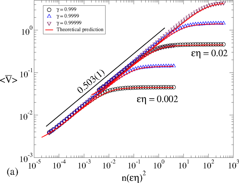
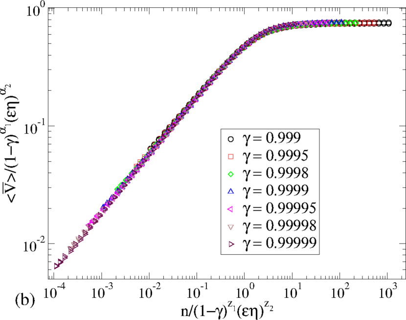
Figure 3: (a) Plot of $<\overline{V}>~{}vs.~{}n$ for different values of $\gamma$ and two combinations of $\eta\varepsilon$. (b) Overlap of the curves shown in (a) onto a single and universal plot after the following scaling transformations: $n\rightarrow n/[(1-\gamma)^{z_{1}}(\eta\varepsilon)^{z_{2}}]$ and $<\overline{V}>\rightarrow<\overline{V}>/[(1-\gamma)^{\alpha_{1}}(\eta\varepsilon)^{\alpha_{2}}]$. The straight line gives the theoretical prediction [Eq. (40)].

From Fig. 3(a) we see two different kinds of behaviors. At small $n$, the average velocity grows to start with to a power law and eventually it bends towards a regime of saturation for large $n$. The change from growth to the saturation is given by a characteristic crossover $n_{x}$. We notice that a transformation $n\rightarrow n(\eta\varepsilon)^{2}$ coalesces all curves to grow together before moving to the saturation. The behavior shown in Fig. 3(a) allows us to propose that: (i) For short $n$, say $n\ll n_{x}$, the growth regime is described by $<\overline{V}>\propto[(\eta\varepsilon)^{2}n]^{\beta}$ where $\beta$ is the acceleration exponent; (ii) For large enough $n$, typically $n\gg n_{x}$ we have $<\overline{V}_{sat}>\propto(1-\gamma)^{\alpha_{1}}(\eta\varepsilon)^{\alpha_{2}}$ where $\alpha_{1}$ and $\alpha_{2}$ are the saturation exponents; (iii) The crossover $n_{x}$ that marks the changeover from growth to the saturation is given by $n_{x}\propto(1-\gamma)^{z_{1}}(\eta\varepsilon)^{z_{2}}$ where $z_{1}$ and $z_{2}$ are crossover exponents.

The three previous hypotheses allow us to describe the behavior of $<\overline{V}>$ by a homogeneous function of the type

$$<\overline{V}> [ (\eta\varepsilon)^{2}n,\eta\varepsilon,(1-\gamma)~{}]=$$ (36)

$$l<\overline{V}>[l^{a}(\eta\varepsilon)^{2}n,l^{b}\eta\varepsilon,l^{d}(1-\gamma)],$$

where $l$ is a scale factor, $a$, $b$ and $d$ are characteristic exponents that in principle must be related to the scaling exponents. A straightforward calculation gives the two scaling laws

$$z_{1}={{\alpha_{1}}\over{\beta}},~{}~{}~{}~{}~{}~{}~{}~{}z_{2}={{\alpha_{2}}\over{\beta}}-2.$$ (37)

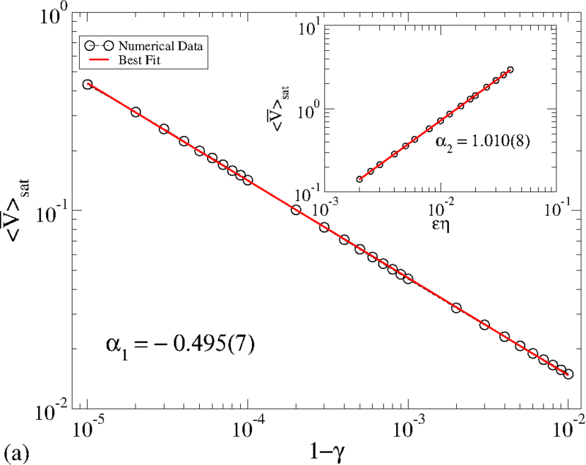
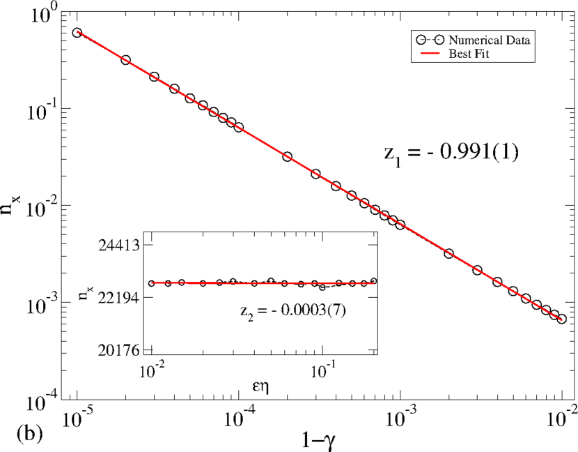
Figure 4: Behavior of: (a) $<\overline{V}_{sat}>$ and (b) $n_{x}$ as a function of $(1-\gamma$). The inset shown the behavior of $<\overline{V}_{sat}>$ and $n_{x}$ for different values of $\varepsilon\eta$.

All the five exponents can be obtained numerically. A power law fitting in the regime of growth for $<\overline{V}>$ gives $\beta=0.503(1)\simeq 1/2$. Similar values were obtained for all curves we simulated for the range of $\gamma\in[0.999,0.99999]$. If we keep fixed $\eta\varepsilon$ and vary $\gamma$, a power law fitting for $<\overline{V}_{sat}>~{}vs.~{}(1-\gamma)$ furnishes $\alpha_{1}=-0.495(7)\cong-1/2$, as shown in Fig. 4 (a). A fitting to the plot of ${n}_{x}~{}vs.~{}(1-\gamma)$ gives $z_{1}=-0.991(1)\cong-1$. Finally if we keep constant $(1-\gamma)$ a fitting to the behavior of $<\overline{V}_{sat}>~{}vs.~{}\eta\varepsilon$ gives $\alpha_{1}=1.010(8)\cong 1$ while a plot of $n_{x}~{}vs.~{}\eta\varepsilon$ yields $z_{2}=-0.0003(7)\cong 0$. When the two scaling laws (37) are used to check the exponents, the results obtained are remarkably in well agreement with the simulations.

III.4 Averaging the velocity along $n$

As given by Eq. (30), the squared velocity was obtained considering an average over an ensemble of particles. However, the simulations were made using either ensemble average as well as average on time. Therefore, we have to find a corresponding expression of the squared velocity when it is also averaged over the number of collisions $n$. The average squared velocity is written as

$$<\overline{V^{2}}(n)>={{1}\over{n+1}}\sum_{i=0}^{n}\overline{V^{2}}(i).$$ (38)

The summation over the exponential terms converges since their arguments are negative. The convergence of the exponential terms is

$$\sum_{i=0}^{n}e^{({{\gamma^{2}-1}\over{2}})i}=\left[{{1-e^{({{\gamma^{2}-1}\over{2}})(n+1)}}\over{1-e^{{\gamma^{2}-1}\over{2}}}}\right],$$ (39)

hence the root mean squared velocity is written as $V_{rms}(n)=\sqrt{<\overline{V^{2}}(n)>}$, therefore

$$V_{rms}(n)=\sqrt{{{(1+\gamma)\eta^{2}\varepsilon^{2}}\over{4(1-\gamma)}}+{{1}\over{(n+1)}}\left[V_{0}^{2}-{{(1+\gamma)\eta^{2}\varepsilon^{2}}\over{4(1-\gamma)}}\right]\left[{{1-e^{{(n+1){{(\gamma^{2}-1)}\over{2}}}}}\over{1-e^{{{(\gamma^{2}-1)}\over{2}}}}}\right]}.$$ (40)

A plot of Eq. (40) is represented as a continuous line in Fig. 3(a).

Two important limits for Eq. (40) are:

1. $n=0$, that leads to $V_{rms}(0)=V_{0}$;

2. Considering the limit of $n\rightarrow\infty$, we have

   $$V_{rms}(n\rightarrow\infty)=\sqrt{{{(1+\gamma)\eta^{2}\varepsilon^{2}}\over{4(1-\gamma)}}}.$$ (41)

With Eq. (40) we can discuss the behavior of $V_{rms}$ for short $n$. In the limit of $\gamma\approx 1$ we can Taylor expand the two exponentials of Eq. (40). Because of term $(n+1)$ in the denominator of Eq. (40), the expansion of the exponential of the numerator must go until second order while the denominator can go only to the first. Grouping the terms properly we obtain the expression of $V_{rms}(n)$ when $V_{0}\cong 0$ as

$$V_{rms}(n)\cong{{(1+\gamma)\eta\varepsilon}\over{4}}\sqrt{(n+1)}.$$ (42)

When $n\gg 1$ such that $\sqrt{(n+1)}\cong\sqrt{n}$ then we have $V_{rms}(n)\cong{{(1+\gamma)\eta\varepsilon}\over{4}}\sqrt{n}$.

III.5 Critical exponents

The five relevant critical exponents that describe the scaling properties of the average velocity curves are $\beta$, $\alpha_{i}$ and $z_{i}$ with $i=1,2$. The exponents $\alpha_{1}$ and $\alpha_{2}$ are obtained for the regime of $n\rightarrow\infty$. From Eq. (41) we obtain $\alpha_{1}=-1/2$ and $\alpha_{2}=1$. The exponent $\beta$ comes from Eq. (42). When $n\gg 1$ we have $\beta=1/2$. Finally, the crossover iteration number $n_{x}$ can be estimated when Eq. (42) intersects Eq. (41). A straightforward calculation gives

$$n_{x}={{4}\over{(1+\gamma)}}(1-\gamma)^{-1}.$$ (43)

Then we conclude that $z_{1}=-1$ and $z_{2}=0$.

III.6 Velocity distribution

Let us discuss here how is the shape of the velocity distribution for the dynamics in the dissipative case. It is important to notice that the lowest velocity for a moving particle is limited to the lowest velocity of the moving boundary, hence $V_{l}=-\eta\epsilon$. Upward velocities are unbounded but unlimited energy growth is not observed due to the dissipation. The lower limit for the velocity plays a major rule on the distribution of the velocity and to illustrate this we discuss the following case. Suppose an ensemble of initial conditions with different angular variables, $\alpha$, $\theta$, but with the same initial velocity is given. The initial velocity is chosen in such a way that it is located in a region above of lower velocity limit and, at the same time, below than the saturation. The dynamics evolves as follows. For short number of collision with the boundary, part of the ensemble of particles raises the velocity while the other part reduces velocity. This distribution is Gaussian, as shown in Fig. 5 in blue (dark gray) color for and initial velocity of $V_{0}=0.2$ and distribution collected after $10$ collisions with the boundary.

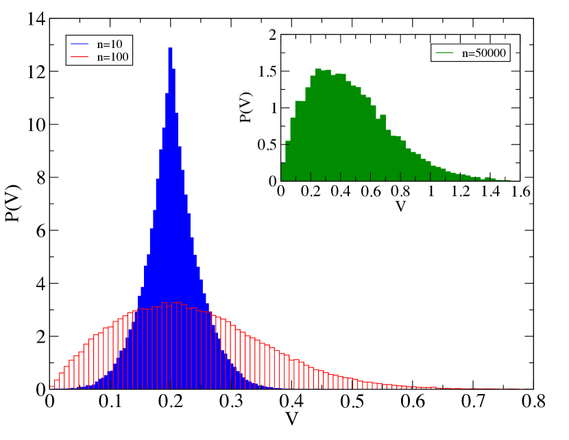
Figure 5: Plot of the normalized probability distribution for the velocity for an ensemble of $10^{5}$ particles in the dissipative and stochastic oval billiard. Blue (dark gray) was obtained after $10$ collisions while red bars (light gray) was obtained after $100$ collisions. The in-box was obtained after $50,000$ collisions. The initial velocity used was $V_{0}=0.2$ and control parameters $\epsilon\eta=0.02$ and $\gamma=0.999$ for $p=2$.

The parameters used were $\epsilon\eta=0.02$, $\gamma=0.999$ and $p=2$, although other values would lead to similar results. Moreover, a total of $2.5\times 10^{6}$ different initial conditions were considered in the ensemble. As soon as the dynamics evolves, the Gaussian distribution flats itself in both sides until the left hand side curves touches the lower limit of the velocity. See the red (light gray) bars obtained for the distribution after $100$ collisions with the boundary. At this point, the distribution experiences a break of symmetry and hence if the initial velocity of the distribution is lower that the saturation, the average velocity starts to grow until approaches the saturation. From this point of symmetry break and beyond this point, the distribution is not Gaussian anymore and it has similar shape as shown in the in-box of Fig. 5. Such distribution was obtained after $50,000$ collisions of the ensemble of particles with the boundary. Although the distribution is not Gaussian anymore due to the break of symmetry at $V=V_{l}$, the distribution has clearly a peak and decays monotonically for large enough values of velocity warranting convergence for the average velocity as well other momenta of the distribution. It is worth to mention that such a break in the symmetry in the probability distribution was previously observed for a one dimensional Fermi Ulam model physicaa . There, the authors show that the velocity/energy distribution can be described perfectly by a folded normal distribution.

IV Connection between the two approaches

The results discussed in Section II involving the heat transfer equation were obtained as a function of the time $t$ while in Section III the results were discussed using the number of collisions $n$. It is important to mention that the time $t$ and the number of collisions $n$ are variables not trivially connected with each other. It happens because a particle moving with high speed can experience many more collisions with the boundary when compared with a particle with low energy at the same interval of time. In this section we discuss a way to make a connection of the two variables therefore linking the results discussed in Secs. II and III.

Given the particle travels with constant velocity between collisions, the length of time between two collisions is $\Delta t=d/|\vec{V}|$ where $d$ is the distance traveled by the particle and $|\vec{V}|$ is its absolute velocity. Therefore, the total time spent at $n$ collisions is written as

$$\tau=\sum_{i=0}^{n}{{d_{i}}\over{|\vec{V}_{i}|}}.$$ (44)

The summation in Eq. (44) seems to be not easy to be made. As an attempt to have an explicit expression involving the relevant parameters of the system considered we will do the summation in two stages evaluating then the numerator separately then the denominator.

From the numerator we can estimate the mean free path, which we represent as

$$\overline{d}={{1}\over{(n+1)}}\sum_{i=0}^{n}d_{i},$$ (45)

where $d_{i}$ is defined as the distance from two collisions as

$$d_{i}=\sqrt{[x(\theta_{i+1})-x(\theta_{i})]^{2}+[y(\theta_{i+1})-y(\theta_{i})]^{2}},$$ (46)

where $x(\theta)=R(\theta)\cos(\theta)$ and $y(\theta)=R(\theta)\sin(\theta)$. The dynamics of each particle is chaotic, therefore when we do an average over $\theta\in[0,2\pi]$ we obtain

$$\overline{d}=\sqrt{2+\eta^{2}\left[1+{{\varepsilon^{2}}\over{2}}\right]}.$$ (47)

The second part we have to consider is $\sum_{i=0}^{n}{{1}\over{V_{i}}}$. To do that we consider the variation of the velocity from the collision $i$ to $(i+1)$ is small so that the summation can be approximated by

$$\sum_{i=0}^{n}{{1}\over{V_{i}}}\cong\int_{0}^{n}{{1}\over{V(n^{\prime})}}dn^{\prime}.$$ (48)

The expression for $\tau$ obtained for the explicit form of $\overline{V}$ as shown in Eq. (31) is not an easy equation to deal with and the result is reported in the Appendix 2 for the interested reader. Instead of dealing with the whole equation we consider an easier approach. As discussed in Ref. diego , the behavior of the average squared velocity, when settled in scaling variables can be described by a function of the type

$$f(x)=\left[{{x}\over{1+x}}\right]^{\beta},$$ (49)

where $\beta$ is the accelerating exponent. In our case $\beta=1/2$. Therefore, the scaled variables considered are: $f\rightarrow{{\overline{V}\sqrt{(1-\gamma)}}\over{\eta\varepsilon}}$ and $x\rightarrow n(1-\gamma)$. Incorporating these two equations as the behavior of $\overline{V}(n)$ we end up with the following equation to be solved

$$\tau={{\overline{d}\sqrt{(1-\gamma)}}\over{\eta\varepsilon}}\int{{dn}\over{\sqrt{{n(1-\gamma)}\over{1+n(1-\gamma)}}}},$$ (50)

After doing the integration (see Appendix 3 for the result of the integral) and keeping only the leading term in $n$ we obtain

$$\tau\cong{{\overline{d}\sqrt{(1-\gamma)}}\over{\eta\varepsilon}}n.$$ (51)

V Conclusions

We have studied some dynamical and statistical properties of gas of non interacting particles in a time dependent and dissipative oval billiard. We have investigated the behavior of the average velocity of the particles as a function of time and the number of collisions with the moving boundary by using two different approaches, namely, involving (i) heat transfer and (ii) billiards. We have obtained an empirical expression for the average squared velocity by using the equilibrium condition at the steady state regime. Such an expression allowed us to make a connection with the thermodynamic, more precisely by using the Fourier law for heat transfer. The resulting equation have shown that the temperature of the gas reaches the thermal equilibrium for sufficiently long time. Our results also have demonstrated that the average squared velocity grows as a power law and after a crossover it tends to a constant plateau. Furthermore, the stronger is the dissipation the faster is the transition from growth to saturation. Finally, by using an empirical function to describe the behavior of the average squared velocity, we have shown that time and number of collisions are linearly correlated.

Appendix 1

This appendix is devoted to a short discussion on the heat flow equation blu . The heat can indeed quantify an amount of energy which is transferred due to a temperature gradient. The amount of heat flowing along the temperature gradient depends on the thermal conductivity $\kappa$. The heat flows from a region of high to low temperature, therefore this flow is contrary to the temperature gradient. In a generic 3-D system, the heat flux vector $\vec{J}$ is written as $\vec{J}=-\kappa A\vec{\nabla}T$, where $A$ corresponds to a section of area perpendicular to where the flow of heat is flowing while $\vec{\nabla}T$ gives the gradient of temperature. The signal $(-)$ is introduced to represent a flow contrary to the temperature gradient, i.e. from higher to lower temperature. The vector $\vec{J}$ indeed represents a certain amount of energy which is flowing through an area $A$ at a given interval of time due to a gradient of temperature.

In the system we are considering in this paper, the flow of heat is not crossing a perpendicular area, but rather it crosses the border of the billiard. Hence, in the case 2-D as discussed, the heat transfer equation is written as

$$J={{\partial Q}\over{\partial t}}=-\kappa\ell{{\partial T}\over{\partial x}},$$ (52)

where $J$ represents the amount of heat which is transferred around the border $\ell$ of the billiard at a given instant of time due to a temperature gradient represented as ${{\partial T}\over{\partial x}}$. In our case, the thermal conductivity coefficient $\kappa$ denotes the constant of proportionality between the amount of energy flowing in the border of the billiard $\ell$ per unit of time due to a temperature gradient.

Appendix 2

When we consider $V(n)$ as given by Eq. (31) to obtain the expression for $\tau$ the direct integral is

$$\tau=\overline{d}\int_{0}^{n}{{dn^{\prime}}\over{\sqrt{\overline{V^{2}_{0}}e^{{{(\gamma^{2}-1)}\over{2}}n^{\prime}}+{{(1+\gamma)}\over{4(1-\gamma)}}\eta^{2}\varepsilon^{2}\bigg{[}1-e^{{{(\gamma^{2}-1)}\over{2}}n^{\prime}}\bigg{]}}}}.$$ (53)

A straight integration yields

$$\tau={{8\sqrt{2+\eta^{2}\left(1+{{\varepsilon^{2}}\over{2}}\right)}}\over{\eta\varepsilon\sqrt{(1+\gamma)}(1-\gamma^{2})}}\times\left[{\rm arctanh}\left({{\sqrt{{{(1+\gamma)\eta^{2}\varepsilon^{2}}\over{4(1-\gamma)}}+\left(V_{0}^{2}-{{(1+\gamma)\eta^{2}\varepsilon^{2}}\over{4(1-\gamma)}}\right)e^{{{(\gamma^{2}-1)}\over{2}}n}}}\over{{{\eta\varepsilon}\over{2}}\sqrt{{(1+\gamma)}\over{(1-\gamma)}}}}\right)-{\rm arctanh}\left({{V_{0}}\over{{{\eta\varepsilon}\over{2}}\sqrt{{{(1+\gamma)}\over{(1-\gamma)}}}}}\right)\right].$$

With some algebra one can isolate $n$ as a function of $\tau$ from the equation above.

Appendix 3

The solution of the integral

$$\tau={{\overline{d}\sqrt{(1-\gamma)}}\over{\eta\varepsilon}}\int{{dn}\over{\sqrt{{n(1-\gamma)}\over{1+n(1-\gamma)}}}},$$ (54)

is given by

$$\tau={{\overline{d}\sqrt{(1-\gamma)}}\over{\eta\varepsilon}}\left[{{1}\over{2}}{{2\sqrt{(n^{2}-n^{2}\gamma+n)}\sqrt{(1-\gamma)}}\over{\sqrt{(1-\gamma)}\sqrt{-n(-1-n+n\gamma)}\sqrt{{{-n(1-\gamma)}\over{-1-n+n\gamma}}}}}n\right]+{{\overline{d}\sqrt{(1-\gamma)}}\over{\eta\varepsilon}}\left[{{1}\over{2}}{{\ln\left[-{{1}\over{2}}\left({{-1-2n+2n\gamma-2\sqrt{(n^{2}-n^{2}\gamma+n)}\sqrt{1-\gamma}}\over{\sqrt{(1-\gamma)}}}\right)\right]}\over{\sqrt{(1-\gamma)}\sqrt{-n(-1-n+n\gamma)}\sqrt{{{-n(1-\gamma)}\over{-1-n+n\gamma}}}}}n\right].$$ (55)

After grouping the terms and considering only the leading term we have

$$\tau={{\overline{d}\sqrt{(1-\gamma)}}\over{\eta\varepsilon}}\left[n\sqrt{1+{{1}\over{n(1-\gamma)}}}~{}\right].$$ (56)

Expanding the square root and keeping only the first order we have

$$\tau={{\overline{d}\sqrt{(1-\gamma)}}\over{\eta\varepsilon}}\left[n+{{1}\over{2(1-\gamma)}}\right],$$ (57)

therefore

$$\tau\cong{{\overline{d}\sqrt{(1-\gamma)}}\over{\eta\varepsilon}}n.$$ (58)

References

- (1) G. Birkhoff, Dynamical Systems, American Mathematical Society, Providence, RI, USA, 1927.
- (2) Ya. G. Sinai, Russian Mathematical Surveys, 25, 137 (1970).
- (3) Ya G. Sinai, Not. Am. Math. Soc. 51 412 (2004).
- (4) L. A. Bunimovich, Functional Analysis and Its Applications, 8, 73 (1974).
- (5) L. A. Bunimovich and Ya. G. Sinai, Communications in Mathematical Physics, 78, 479 (1981).
- (6) N. Chernov and R. Markarian, Chaotic Billiards. American Mathematical Society, Vol. 127, 2006.
- (7) L. A. Bunimovich, Commun. Math. Phys., 65, 295 (1979).
- (8) L. A. Bunimovich, Chaos 1, 187 (1991).
- (9) L. A. Bunimovich and L. V. Vela-Arevalo, Chaos, 22, 026103 (2012).
- (10) S. Tabachnikov, Geometry and Billiards (Providence, RI: American Mathematical Society) (2005).
- (11) C. P. Dettmann and O. Georgiou, Physica D 238, 2395-2403 (2009).
- (12) C. P. Dettmann and O. Georgiou, J. Phys. A.: Math. Theor. 44, 195102, (2011).
- (13) M. Robnik, Nonlinear Phenomena and Chaos (Bristol: Hilger) 303 (1986).
- (14) D. P. Sanders, Phys. Rev. E 71, 016220 (2005).
- (15) A. Bäcker, R. Ketzmerick, S. Löck, M. Robnik, G. Vidmar, R. Höhmann, U. Kuhl, H.-J. Stöckmann, Phys. Rev. Lett. 100, 174103 (2008).
- (16) D. F. M. Oliveira, M. Robnik, Int. J. Bif. Chaos, 22, 1250207 (2012).
- (17) A. B. Ryabov and A. Loskutov. J. Phys. A: Math. Theor., 43, 125104 (2010).
- (18) V. Gelfreich, D. Turaev, J. Phys. A 41, 212003 (2008).
- (19) V. Gelfreich, D. Turaev, Comm. Math. Phys. 283, 769 (2008).
- (20) E. Fermi, Phys. Rev, 75, 1169 (1949).
- (21) A. Loskutov, A. B. Ryabov and L. G. Akinshin, J. Phys. A, 33, 7973 (2000).
- (22) A. Loskutov, A. B. Ryabov and L. G. Akinshin, J. Exp. and Theor. Physics, 89, 966 (1999).
- (23) A. K. Karlis, P. K. Papachristou, F. K. Diakonos, V. Constantoudis, P. Schmelcher, Phys. Rev. E, 76 016214 (2007).
- (24) D. F. M. Oliveira, E. D. Leonel, Chaos 22, 026123 (2012).
- (25) E. D. Leonel, D. F. M. Oliveira and A. Loskutov, Chaos, 19, 033142 (2009).
- (26) C. P. Dettmann and O. Georgiou, Phys. Rev. E, 83, 036212 (2011).
- (27) R. E. de Carvalho, F. C. de Souza and E. D. Leonel, J. Phys. A: Math. Gen., 39, 3561 (2006).
- (28) F. Lenz, F. K. Diakonos and P. Schmelcher, Phys. Rev. Lett., 100, 014103 (2008).
- (29) F. Lenz, C. Petri, F. R. N. Koch, F. K. Diakonos and P. Schmelcher, New J. Phys., 11, 083035 (2009).
- (30) M. V. Berry, Eur. J. Phys. 2, 91 (1981).
- (31) D. F. M. Oliveira and E. D. Leonel, Physica A 389, 1009 (2010)
- (32) E. D. Leonel and L. A. Bunimovich, Phys. Rev. Lett., 104, 224101 (2010).
- (33) S. J. Blundell, K. M. Blundell, Concepts in thermal physics, 493. Oxford University Press, Oxford (2010).
- (34) A. Loskutov, O. Chichigina, A. Ryabov, Int. J. Bif. Chaos, 18, 2863 (2008).
- (35) D. F. M. Oliveira, M. Robnik, E. D. Leonel, Phys. Lett. A, 376, 723 (2012).
- (36) D. F. M. Oliveira, Mario R. Silva, E. D. Leonel, Physica A, 436, 909 (2015).