Collider signals of $W^{\prime}$ and $Z^{\prime}$ bosons
in the gauge-Higgs unification

Abstract

In the $SO(5)\times U(1)$ gauge-Higgs unification (GHU), Kaluza-Klein (KK) excited states of charged and neutral vector bosons, $W^{(1)}$, $W_{R}^{(1)}$, $Z^{(1)}$, $\gamma^{(1)}$ and $Z_{R}^{(1)}$, can be observed as $W^{\prime}$ and $Z^{\prime}$ signals in collider experiments. In this paper we evaluate the decay rates of the $W^{\prime}$ and $Z^{\prime}$, and $s$-channel cross sections mediated by $W^{\prime}$ and $Z^{\prime}$ bosons with final states involving the standard model (SM) fermion pair ($\ell\nu$, $\ell\bar{\ell}$, $q\bar{q}^{\prime}$), $WH$, $ZH$, $WW$ and $WZ$. $W^{\prime}$ and $Z^{\prime}$ resonances appear around $6.0$ TeV ($8.5$ TeV) for $\theta_{H}=0.115$ (0.0737) where $\theta_{H}$ is the Aharonov-Bohm phase in the fifth dimension in GHU. For decay rates we find $\Gamma(W^{\prime}\to WH)\simeq\Gamma(W^{\prime}\to WZ)$ ($W^{\prime}=W^{(1)}$, $W_{R}^{(1)}$), $\Gamma(W^{(1)}\to WH,WZ)\sim\Gamma(W_{R}^{(1)}\to WH,WZ)$, $\Gamma(Z^{(1)}\to ZH)\simeq\sum_{Z^{\prime}=Z^{(1)},\gamma^{(1)}}\Gamma(Z^{\prime}\to WW)$, and $\Gamma(Z_{R}^{(1)}\to ZH)\simeq\Gamma(Z_{R}^{(1)}\to WW)$. $W^{\prime}$ and $Z^{\prime}$ signals of GHU can be best found at the LHC experiment in the processes $pp\to W^{\prime}(Z^{\prime})+X$ followed by $W^{\prime}\to t\bar{b}$, $WH$, and $Z^{\prime}\to e^{+}e^{-}$, $\mu^{+}\mu^{-},ZH$ near the $W^{\prime}$ and $Z^{\prime}$ resonances. For the lighter $Z^{\prime}$ ($\theta_{H}=0.115$) case, with forthcoming 30 fb^-1 data of the 13 TeV LHC experiment we expect about ten $\mu^{+}\mu^{-}$ events for the invariant mass range 3000 to 7000 GeV, though the number of the events becomes much smaller when $\theta_{H}=0.0737$. In the process with $WZ$ in the final state, it is confirmed that the leading contributions in the amplitude from the longitudinal polarizations of $W$ and $Z$ in the $s$-, $t$- and $u$-channels cancel with each other so that the unitarity is preserved, provided that all KK excited states in the intermediate states are taken into account. Deviation of the $WWZ$ coupling from the SM is very tiny. Exotic partners $t_{T}^{(1)}$ and $b_{Y}^{(1)}$ of the top and bottom quarks with electric charge $+5/3$ and $-4/3$ have mass $M_{t_{T}^{(1)},b_{Y}^{(1)}}=4.6$ TeV ($5.4$ TeV) for $\theta_{H}=0.115$ ($0.0737$), becoming the lightest non-SM particles in GHU which can be singly produced in collider experiments.

1 Introduction

At the LHC, $W^{\prime}$ and $Z^{\prime}$ are searched with various decay modes: decay to lepton pairs ($\ell\bar{\ell}$, $\ell\nu$, $\nu\bar{\nu}$) Aaboud:2016cth ; CMS:2016abv ; ATLAS:2014wra ; Chatrchyan:2013lga ; Khachatryan:2015pua ; Aaboud:2016zkn , a pair of top and bottom Aad:2014xra ; Aad:2014xea ; Chatrchyan:2012gqa , $q\bar{q}$-dijet Aad:2015eha ; ATLAS:2015nsi , $WH(\to\ell\nu b\bar{b})$ and $ZH(\to\ell\bar{\ell}b\bar{b})$ Khachatryan:2015bma ; Khachatryan:2016yji ; Aaboud:2016lwx ; Khachatryan:2016cfx and $WW$ and $WZ$ Aad:2015ipg ; Chatrchyan:2012rva ; Khachatryan:2014hpa ; Khachatryan:2014xja ; Aad:2015owa ; ATLAS-CONF-2015-068 ; ATLAS-CONF-2015-073 . In the models with extra dimensions, $W^{\prime}$ and $Z^{\prime}$ appear as Kaluza-Klein (KK) excited states of charged and neutral vector bosons. The couplings of $W^{\prime}$ and $Z^{\prime}$ to fields in the standard model (SM) depend on the details of the models. For example, in the minimal universal extra dimension (mUED) model Appelquist:2000nn , the conservation of KK number forbids tree-level couplings of KK-excited states to the SM fields so that production of $W^{\prime}$ or $Z^{\prime}$ in the collider experiment is highly suppressed.

Non-vanishing couplings of $W^{\prime}$ and $Z^{\prime}$ to the SM fields in models with extra-dimensions originate from the violation of the KK number conservation which reflects the translational invariance in the direction of the extra dimensional space. The KK number conservation is broken by, for instance, domain-wall like bulk mass terms, brane localized mass terms to the fermion, or warped extra dimensions. It is well known that in the models in which SM fields live in the warped bulk space, couplings among fermions and KK-excited gauge bosons are non-vanishing and can be large. In the minimal $SU(3)$ gauge-Higgs unification (GHU) model Kubo:2001zc there are no $W^{\prime}$ or $Z^{\prime}$ couplings to the SM fields. In a custodially-protected warped extra dimensional model Angelescu:2015yav , $WW$ and $WH$ diboson signals have been studied.

The GHU provides a natural scenario for solving the gauge hierarchy problem. Many advances have been made in this direction recently Kubo:2001zc ; Hosotani:1983xw ; Davies1988 ; Hosotani1989a ; Hatanaka:1998yp ; Hatanaka:1999sx ; Scrucca:2003ra ; Haba:2004qf ; Agashe2005 ; Medina2007 ; Hosotani:2006qp ; Sakamura:2006rf ; Hosotani:2007qw ; Hosotani:2007kn ; Hosotani:2008tx ; Hosotani:2008by ; Haba:2009hw ; Hosotani:2009qf ; Serone:2009kf ; Hosotani:2010hx ; Hosotani:2011vr ; Hasegawa2013 ; Funatsu:2013ni ; Funatsu:2014fda ; Funatsu:2014tka ; Funatsu:2015xba ; Burdman2003 ; HHKY2004 ; Lim2007 ; Kojima:2011ad ; Yamamoto2014 ; Kakizaki2014 ; Sakamura2014 ; Kitazawa2015 ; HY2015a ; Yamatsu2016a ; Sakamura2016 ; Furui:2016owe ; Adachi:2016zdi ; Hasegawa:2016spd ; Kojima:2016fvv ; Hosotani2016b ; deAnda:2014dba ; Cossu:2013ora ; Forcrand2015 ; Knechtli2016 ; HH-flat . In the present paper, we evaluate couplings of KK excited gauge bosons to the SM gauge boson, Higgs boson, and fermions, and study collider signals of $W^{\prime}$ and $Z^{\prime}$ in the $SO(5)\times U(1)$ GHU model which naturally incorporates the Higgs boson of mass $m_{H}=125$ GeV and gives almost the same phenomenology as the SM at low energies Funatsu:2013ni ; Funatsu:2014fda ; Funatsu:2014tka ; Funatsu:2015xba . In the previous work Funatsu:2014fda , we reported that in hadron collider experiments large $Z^{\prime}$ signals are expected due to the large couplings of right-handed fermions to the KK-excited gauge bosons Gherghetta:2000qt . In the present paper we evaluate cross sections not only with fermionic final states but also with bosonic $WH$, $ZH$, $WW$ and $WZ$ final states.

In the warped space, in general, it is difficult to evaluate couplings among various fields as they should be calculated in their mass eigenstates. One remarkable feature of the GHU is that the Higgs VEV can be eliminated by a large gauge-transformation and its effect is transmitted to the change in the boundary conditions so that one can obtain mass eigenstates easily. In the previous work Funatsu:2015xba , it is found that KK non-conserving couplings $HW^{(m)}W^{(n)}$ and $ZW^{(m)}W^{(n)}$ ($m\neq n$), including $HWW^{(n)}$ and $ZWW^{(n)}$, are non-vanishing, and we used them in the calculation of the $H\to Z\gamma$ decay rate .

This paper is organized as follows. In Sec. 2, the model is introduced . In Sec. 3 decay width and cross sections formulas are given. In Sec. 4 we introduce effective theories to qualitatively describe salient relations among various decay widths. In Sec. 5, couplings and decay widths of $W^{\prime}$ and $Z^{\prime}$ are evaluated in GHU. In Sec. 6 cross sections are evaluated. $W^{\prime}$ and $Z^{\prime}$ signals in $pp$ collision experiment at LHC are explored. We also show how the unitarity in the process $d\bar{u}\to WZ$ is ensured by including contributions from KK states of vector bosons and fermions in the intermediate states. Sec. 7 is devoted to summary. In Appendix A $SO(5)$ generators and basis functions in the analysis are summarized. In Appendices B and C masses and wave functions for bosonic and fermionic KK states are given, respectively. In Appendix D fermion couplings to vector bosons and the Higgs boson are summarized, whereas cubic vector couplings and Higgs couplings are given in Appendix E. In Appendices F and G, formulae for decay widths and scattering cross sections are summarized, respectively.

2 Model

We consider five-dimensional (5D) gauge theory in the Randall-Sundrum space-time, whose metric is

$$ds^{2} = e^{-2\sigma(y)}\eta_{\mu\nu}dx^{\mu}dx^{\nu}+dy^{2}=G_{MN}dx^{M}dx^{N},$$ (2.1)

where $\eta_{\mu\nu}={\mathop{\mbox{diag}}\nolimits}(-1,1,1,1)$. Here $\sigma(y)=k|y|$ for $-L\leq y\leq L$ and $\sigma(y+2L)=\sigma(y)$ is satisfied. $k$ is the $AdS_{5}$ curvature. $y=0$ and $y=L$ boundaries are referred to as the UV (ultraviolet) and IR (infrared) branes, respectively. The Kaluza-Klein (KK) mass scale is given by

$$m_{KK} \equiv \frac{\pi k}{e^{kL}-1},$$ (2.2)

and when $kL\gtrsim 5$, it is followed by $m_{KK}\ll k$, $L^{-1}$.

This space-time has symmetric under the $Z_{2}$ reflection $y\to-y$, and fundamental region of the extra dimension is given by $0\leq y\leq L$. In this region we introduce a new coordinate $z=e^{ky}$, with which the metric becomes

$$ds^{2} = \frac{1}{z^{2}}\left(\eta_{\mu\nu}dx^{\mu}dx^{\nu}+\frac{dz^{2}}{k^{2}}\right).$$ (2.3)

Note that $\partial_{y}=kz\partial_{z}$ and $V_{y}=kzV_{z}$ for a vector field $V_{M}$.

In the 5D bulk space there are $SO(5)$ and $U(1)_{X}$ gauge fields, four $SO(5)$-vector fermions per generation $\Psi_{a}^{{g}}$ ($a=1,2,3,4$, ${g}=1,2,3$), and $N_{F}$ $SO(5)$-spinor fermions $\Psi_{F_{i}}$ ($i=1,\cdots,N_{F}$). We note that each of $\Psi_{1}$ and $\Psi_{2}$ is an $SU(3)$-color triplet.

The bulk part of the action is given by

$$S_{\rm bulk} = \int d^{5}x\sqrt{-G}\biggl{\{}-\frac{1}{2}{\mathop{\mbox{tr}}\nolimits}G^{MR}G^{NS}F_{MN}^{(A)}F^{(A)}_{RS}-\frac{1}{4}G^{MR}G^{NS}F^{(B)}_{MN}F^{(B)}_{RS}$$ (2.4)

$$+\frac{1}{2\xi_{(A)}}(f_{\rm gf}^{(A)})^{2}+\frac{1}{2\xi_{(B)}}(f_{\rm gf}^{(B)})^{2}+{\cal L}_{GH}^{(A)}+{\cal L}_{GH}^{(B)}$$

$$+\sum_{{g}=1}^{3}\sum_{a=1}^{4}\bar{\Psi}^{{g}}_{a}{\cal D}(c^{{g}}_{a})\Psi^{{g}}_{a}+\sum_{i=1}^{N_{F}}\bar{\Psi}_{F_{i}}{\cal D}(c_{F_{i}})\Psi_{F_{i}}\biggr{\}},$$

$${\cal D}(c_{a}) \equiv \Gamma^{A}e_{A}{}^{M}\left(\partial_{M}+\frac{1}{8}\Omega_{MBC}[\Gamma^{B},\Gamma^{C}]-ig_{A}A_{M}-ig_{B}Q_{X,a}-c_{a}k\epsilon(y)\right),$$ (2.5)

where $\epsilon(y)\equiv\sigma^{\prime}/k$ is a sign function. $\Gamma^{M}$ denotes gamma matrices which is defined by $\{\Gamma^{M},\Gamma^{N}\}=2\eta^{MN}$ ($\eta^{55}=+1$). $e_{A}{}^{M}$ is an inverse fielbein, and $\Omega_{MBC}$ is the spin connection. $F_{MN}^{(A)}=\partial_{M}A_{N}-\partial_{N}A_{M}-ig_{A}[A_{M},A_{N}]$ and $F_{MN}^{(B)}=\partial_{M}B_{N}-\partial_{N}B_{M}$. $g_{A}$ and $g_{B}$ are 5D gauge couplings of $SO(5)$ and $U(1)_{X}$, respectively. $g_{w}\equiv g_{A}/\sqrt{L}$ is the four-dimensional (4D) $SO(5)$ coupling. $f_{\rm gf}^{(A)}$ and $f_{\rm gf}^{(B)}$ are gauge-fixing functions, and $\xi_{(A)}$ and $\xi_{(B)}$ are corresponding gauge parameters. ${\cal L}_{GH}^{(A)}$ and ${\cal L}_{GH}^{(B)}$ denote ghost Lagrangians.

Bulk fermions are $SO(5)$-vectors. For the third generation, they are given by

$$\Psi_{1} = \left(\begin{pmatrix}T&t\\ B&b\end{pmatrix},t^{\prime}\right)=((Q_{1},q),t^{\prime})=(\check{\Psi}_{1}^{q},t^{\prime}),$$

$$\Psi_{2} = \left(\begin{pmatrix}U&X\\ D&Y\end{pmatrix},b^{\prime}\right)=((Q_{2},Q_{3}),b^{\prime})=(\check{\Psi}_{2}^{q},b^{\prime}),$$

$$\Psi_{3} = \left(\begin{pmatrix}\nu_{\tau}&L_{1X}\\ \tau&L_{1Y}\end{pmatrix},\tau^{\prime}\right)=((\ell,L_{1}),\tau^{\prime}),=(\check{\Psi}_{3}^{\ell},\tau^{\prime}),$$

$$\Psi_{4} = \left(\begin{pmatrix}L_{2X}&L_{3X}\\ L_{2Y}&L_{3Y}\end{pmatrix},\nu^{\prime}_{\tau}\right)=((L_{2},L_{3}),\nu^{\prime}_{\tau}),=(\check{\Psi}_{4}^{\ell},\nu^{\prime}_{\tau}),$$ (2.6)

where $SO(4)$ vector is embedded in $(\bm{2},\bm{2})$-representation of $SU(2)_{L}\times SU(2)_{R}$ by

$$\begin{pmatrix}\psi_{11}&\psi_{12}\\ \psi_{21}&\psi_{22}\end{pmatrix}=\frac{1}{\sqrt{2}}(\psi_{4}+i\vec{\sigma}\cdot\vec{\psi})i\sigma_{2} = \begin{pmatrix}-i\psi_{1}-\psi_{2}&i\psi_{3}+\psi_{4}\\ i\psi_{3}-\psi_{4}&i\psi_{1}-\psi_{2}\end{pmatrix}.$$ (2.7)

The brane part of the action consists of scalar part $S_{\rm brane}^{\Phi}$ and brane-fermion part $S_{\rm brane}^{\chi}$. The scalar part is given by

$$S_{\rm brane}^{\Phi} = \int d^{5}x\sqrt{-G}\delta(y)[-(D_{\mu}\Phi)^{\dagger}(D^{\mu}\Phi)-\lambda_{\Phi}(|\Phi|^{2}-w^{2})^{2}],$$

$$D_{\mu}\Phi = \left(\partial_{\mu}-i\left\{g_{A}\sum_{a_{R}=1}^{3}A_{\mu}^{a_{R}}T^{a_{R}}+\frac{1}{2}g_{B}B_{\mu}\right\}\right)\Phi.$$ (2.8)

The fermion part of the brane action is

$$S_{\rm brane}^{\chi} = \int d^{5}x\sqrt{-G}\delta(y)\{{\cal L}_{q}+{\cal L}_{\ell}\},$$

$${\cal L}_{q} \equiv \sum_{{g}=1}^{3}\sum_{\alpha=1}^{3}(\hat{\chi}_{\alpha R}^{q,{g}{\dagger}}i\bar{\sigma}^{\mu}D_{\mu}\hat{\chi}_{\alpha R}^{q,{g}})-i\sum_{{g},{g}^{\prime}=1}^{3}\bigl{[}\kappa_{1}^{q,{g}{g}^{\prime}}\hat{\chi}_{1R}^{q,g{\dagger}}\check{\Psi}_{1L}^{q,{g}^{\prime}}\tilde{\Phi}+\tilde{\kappa}^{q,{g}{g}^{\prime}}\hat{\chi}_{2R}^{q,g{\dagger}}\check{\Psi}_{1L}^{q,{g}^{\prime}}\Phi$$

$$+\kappa_{2}^{q,{g}{g}^{\prime}}\hat{\chi}_{2R}^{q,g{\dagger}}\check{\Psi}_{2L}^{{g}^{\prime}}\tilde{\Phi}+\kappa_{3}^{q,{g}{g}^{\prime}}\hat{\chi}_{3R}^{q,g{\dagger}}\check{\Psi}_{2L}^{{g}^{\prime}}\Phi-\text{(H.c.)}\bigr{]},$$

$${\cal L}_{\ell} \equiv \sum_{{g}=1}^{3}\sum_{\alpha=1}^{3}(\hat{\chi}_{\alpha R}^{\ell,{g}{\dagger}}i\bar{\sigma}^{\mu}D_{\mu}\hat{\chi}_{\alpha R}^{\ell,{g}})-i\sum_{{g},{g}^{\prime}=1}^{3}[\tilde{\kappa}^{\ell,{g}{g}^{\prime}}\hat{\chi}_{3R}^{\ell,g{\dagger}}\check{\Psi}_{3L}^{\ell,{g}^{\prime}}\tilde{\Phi}+\kappa_{1}^{\ell,{g}{g}^{\prime}}\hat{\chi}_{1R}^{\ell,g{\dagger}}\check{\Psi}_{3L}^{\ell,{g}^{\prime}}\Phi$$ (2.9)

$$+\kappa_{2}^{\ell,{g}{g}^{\prime}}\hat{\chi}_{2R}^{\ell,{g}{\dagger}}\check{\Psi}_{4L}^{\ell,{g}^{\prime}}\tilde{\Phi}+\kappa_{3}^{\ell,{g}{g}^{\prime}}\hat{\chi}_{3R}^{\ell,{g}{\dagger}}\check{\Psi}_{4L}^{\ell,{g}^{\prime}}\Phi-\text{(H.c.)},$$

$$D_{\mu}\hat{\chi} = \left(\partial_{\mu}-ig_{A}\sum_{a_{L}=1}^{3}A_{\mu}^{a_{L}}T^{a_{L}}-iQ_{X}g_{B}B_{\mu}\right)\hat{\chi},\quad\tilde{\Phi}\equiv i\sigma_{2}\Phi^{*},$$ (2.10)

where

$$\hat{\chi}_{1R}^{q} = \begin{pmatrix}\hat{T}_{R}\\ \hat{B}_{R}\end{pmatrix}_{7/6},\quad\hat{\chi}_{2R}^{q}=\begin{pmatrix}\hat{U}_{R}\\ \hat{D}_{R}\end{pmatrix}_{1/6},\quad\hat{\chi}_{3R}^{q}=\begin{pmatrix}\hat{X}_{R}\\ \hat{Y}_{R}\end{pmatrix}_{-5/6},$$ (2.11)

$$\hat{\chi}_{1R}^{\ell} = \begin{pmatrix}\hat{L}_{1XR}\\ \hat{L}_{1YR}\end{pmatrix}_{-3/2},\quad\hat{\chi}_{2R}^{\ell}=\begin{pmatrix}\hat{L}_{2XR}\\ \hat{L}_{2YR}\end{pmatrix}_{1/2},\quad\hat{\chi}_{3R}^{\ell}=\begin{pmatrix}\hat{L}_{3XR}\\ \hat{L}_{3YR}\end{pmatrix}_{-1/2},$$ (2.12)

are right-handed brane fermions. We note that each of $\hat{\chi}^{q}_{1R}$, $\hat{\chi}^{q}_{2R}$ and $\hat{\chi}^{q}_{3R}$ is an $SU(3)$-color triplet. We also have introduced $3\times 3$ Yukawa coupling matrices $\kappa^{q}_{1,2,3}$, $\kappa^{\ell}_{1,2,3}$, $\tilde{\kappa}^{q}$ and $\tilde{\kappa}^{\ell}$.

2.1 Orbifold symmetry breaking

We impose $Z_{2}$ boundary conditions at boundaries $y=y_{i}$, $y_{0}\equiv 0$, $y_{1}\equiv L$.

$$\begin{pmatrix}A_{\mu}\\ A_{y}\end{pmatrix}(x,y_{i}-y) = P_{i}\begin{pmatrix}A_{\mu}\\ -A_{y}\end{pmatrix}(x,y_{i}+y)P_{i}^{-1},$$ (2.13)

$$\begin{pmatrix}B_{\mu}\\ B_{y}\end{pmatrix}(x,y_{i}-y) = \begin{pmatrix}B_{\mu}\\ -B_{y}\end{pmatrix}(x,y_{i}+y),$$ (2.14)

$$\Psi_{a}(x,y_{i}-y) = \gamma_{5}P_{i}\Psi(x,y_{i}+y)_{a},$$ (2.15)

where

$$P_{0}^{\rm vec}=P_{1}^{\rm vec}={\mathop{\mbox{diag}}\nolimits}(-1,-1,-1,-1,+1),\quad P_{0}^{\rm sp}=P_{1}^{\rm sp} = \begin{pmatrix}\bm{1}&\\ &-\bm{1}\end{pmatrix}$$ (2.16)

in the vector and spinor representations, respectively. These boundary conditions break $SO(5)$ to $SO(4)\simeq SU(2)_{L}\times SU(2)_{R}$. $A_{\mu}^{a_{L},a_{R}}$ and $A_{y}^{\hat{a}}$ are even function against reflections at $y=y_{i}$ and can have their zero-modes. Zero modes of $A_{\mu}^{a_{L},a_{R}}$ are the gauge fields of unbroken $SO(4)$ symmetry.

2.2 Symmetry breaking by brane scalar

Once $\Phi$ develops a VEV

$$\langle\Phi\rangle=\begin{pmatrix}0\\ w\end{pmatrix},$$ (2.17)

$SU(2)_{R}\times U(1)_{X}$ symmetry is broken to $U(1)_{Y}$ After $\Phi$ develops a VEV, the boundary conditions in the original gauge are given by

at $$z=1 : \partial_{z}A_{\mu}^{a_{L}}=\left(\partial_{z}-\frac{\kappa}{2k}\right)A_{\mu}^{1_{R},2_{R}}=\left(\partial_{z}-\frac{\kappa^{\prime}}{2k}\right)A_{\mu}^{3^{\prime}_{R}}=\partial_{z}B_{\mu}^{Y^{\prime}}=0,$$

$$A_{\mu}^{\hat{a}}=A_{\mu}^{\hat{4}}=0,$$

$$A_{z}^{a_{L}}=A_{z}^{a_{R}}+B_{z}=0,\quad\partial_{z}\left(\frac{1}{z}A_{z}^{\hat{a}}\right)=\partial_{z}\left(\frac{1}{z}A_{z}^{\hat{4}}\right)=0,$$

at $$z=z_{L} : \partial_{z}A_{\mu}^{a_{L}}=\partial_{z}A_{\mu}^{a_{R}}=\partial_{z}B_{\mu}^{X}=0,$$ (2.18)

$$A_{\mu}^{\hat{a}}=A_{\mu}^{\hat{4}}=0,$$

$$A_{z}^{a_{L}}=A_{z}^{a_{R}}=B_{z}=0,\quad\partial_{z}\left(\frac{1}{z}A_{z}^{\hat{a}}\right)=\partial_{z}\left(\frac{1}{z}A_{z}^{\hat{4}}\right)=0.$$

Here we have defined

$$\kappa\equiv\frac{g_{A}^{2}w^{2}}{4}=\frac{g_{w}^{2}Lw^{2}}{4},\quad\kappa^{\prime}\equiv\frac{(g_{A}^{2}+g_{B}^{2})w^{2}}{4},$$ (2.19)

and

$$\begin{pmatrix}A_{M}^{3^{\prime}_{R}}\\ B^{Y^{\prime}}_{M}\end{pmatrix}\equiv\begin{pmatrix}c_{\phi}&-s_{\phi}\\ s_{\phi}&c_{\phi}\end{pmatrix}\begin{pmatrix}A_{M}^{3_{R}}\\ B_{M}\end{pmatrix},$$

$$c_{\phi}\equiv\cos\phi=\frac{g_{A}}{\sqrt{g_{A}^{2}+g_{B}^{2}}},\quad s_{\phi}\equiv\sin\phi=\frac{g_{B}}{\sqrt{g_{A}^{2}+g_{B}^{2}}}.$$ (2.20)

where a mixing angle $\phi$ is defined by $\tan\phi\equiv g_{B}/g_{A}$. KK modes of $A_{\mu}^{1,2_{R}}$ and $A_{\mu}^{\prime 3_{R}}$ with $m_{n}\ll w$ obey effectively Dirichlet boundary conditions on the UV brane : $A_{\mu}^{1_{R},2_{R}}=A_{\mu}^{3^{\prime}_{R}}=0$ at $z=1$.

For fermions, non-vanishing $\langle\Phi\rangle$ also induces brane mass terms given by

$$S_{\rm brane}^{\rm mass} = \int d^{5}x\sqrt{-G}\delta(y)\left\{{\cal L}_{\rm quark}^{\rm mass}+{\cal L}_{\rm lepton}^{\rm mass}\right\},$$ (2.21)

$${\cal L}_{\rm quark}^{\rm mass} = \sum_{{g},{g}^{\prime}=1}^{3}\biggl{[}-\sum_{\alpha=1}^{3}i\mu_{\alpha}^{q,{g}{g}^{\prime}}(\hat{\chi}_{\alpha R}^{q,g{\dagger}}Q_{\alpha L}^{{g}^{\prime}}-Q_{\alpha L}^{{g}^{\prime}{\dagger}}\hat{\chi}_{\alpha R}^{q,{g}})-i\tilde{\mu}^{q,{g}{g}^{\prime}}(\hat{\chi}_{2R}^{q,{g}{\dagger}}q_{L}^{{g}^{\prime}}-q_{L}^{{g}^{\prime}{\dagger}}\hat{\chi}_{2R}^{q,{g}})\biggr{]},$$ (2.22)

$${\cal L}_{\rm lepton}^{\rm mass} = \sum_{{g},{g}^{\prime}=1}^{3}\biggl{[}-\sum_{\alpha=1}^{3}i\mu_{\alpha}^{\ell,{g}{g}^{\prime}}(\hat{\chi}_{\alpha L}^{\ell,{g}{\dagger}}L_{\alpha L}^{{g}^{\prime}}-L_{\alpha L}^{{g}^{\prime}{\dagger}}\hat{\chi}_{\alpha R}^{\ell,{g}})-i\tilde{\mu}^{\ell,{g}{g}^{\prime}}(\hat{\chi}_{3R}^{\ell,{g}{\dagger}}\ell_{L}^{{g}^{\prime}}-\ell_{L}^{{g}^{\prime}{\dagger}}\hat{\chi}_{3R}^{\ell,{g}})\biggr{]}.$$ (2.23)

where

$$\frac{\mu_{\alpha}^{q,{g}{g}^{\prime}}}{\kappa_{\alpha}^{q,{g}{g}^{\prime}}}=\frac{\tilde{\mu}^{q,{g}{g}^{\prime}}}{\tilde{\kappa}^{q,{g}{g}^{\prime}}}=\frac{\mu_{\alpha}^{\ell,{g}{g}^{\prime}}}{\kappa_{\alpha}^{\ell,{g}{g}^{\prime}}}=\frac{\tilde{\mu}^{\ell,{g}{g}^{\prime}}}{\tilde{\kappa}^{\ell,{g}{g}^{\prime}}}=w.$$ (2.24)

For $w\gg m_{KK}$, and $\mu_{\alpha},\,\tilde{\mu}\gg\sqrt{m_{KK}}$, exotic fermions couple to brane fermions to become very heavy, so that only quark and leptons remain at low energy.

Since the gauge field $A_{y}$ plays the role of the Higgs boson, the Yukawa couplings of quarks and leptons are diagonal in the flavor space, and flavor mixing can be induced by non-diagonal brane mass terms. For simplicity we assume that all brane mass terms are flavor-diagonal:

$$\mu_{\alpha}^{q,{g}{g}^{\prime}}=\delta^{{g}{g}^{\prime}}\mu_{\alpha}^{q},\quad\mu_{\alpha}^{\ell,{g}{g}^{\prime}}=\delta^{{g}{g}^{\prime}}\mu_{\alpha}^{\ell},\quad\alpha=1,2,3,$$

$$\tilde{\mu}^{q,{g}{g}^{\prime}}=\delta^{{g}{g}^{\prime}}\tilde{\mu}^{q},\quad\tilde{\mu}^{\ell,{g}{g}^{\prime}}=\delta^{{g}{g}^{\prime}}\tilde{\mu}^{\ell}.$$ (2.25)

2.3 Electroweak symmetry breaking

$A_{z}^{\hat{a}}$ ($a=1,2,3$ and $4$) have their zero modes:

$$A_{z}^{\hat{a}}(x,z) = \phi^{a}(x)\sqrt{\frac{2}{k(z_{L}^{2}-1)}}\cdot z+\cdots,$$ (2.26)

(where “$\cdots$” includes higher-KK modes) and can develop a VEV. We assume that $A_{z}$ develops a VEV in the direction of $T^{\hat{4}}$ and we parameterize it by $\langle\phi^{a}\rangle=v_{W}\delta^{4a}$. Then we define the Wilson-line phase parameter $\theta_{H}$ by

$$\exp\left[\frac{i}{2}\theta_{H}(2\sqrt{2}T^{\hat{4}})\right] = \exp\left[ig_{A}\int_{0}^{z_{L}}\langle A_{z}\rangle dz\right],$$ (2.27)

so that we obtain

$$\theta_{H} = \frac{1}{2}g_{A}v_{W}\sqrt{\frac{z_{L}^{2}-1}{k}}\sim\frac{g_{2}v_{W}}{2}\frac{\pi\sqrt{kL}}{m_{KK}},$$ (2.28)

where $g_{w}\equiv g_{A}/\sqrt{L}$ is the 4D $SO(4)\simeq SU(2)_{L}\times SU(2)_{R}$ gauge coupling constant. We also have a formula of $W$-boson mass.

$$m_{W} \simeq \frac{m_{KK}}{\pi\sqrt{kL}}|\sin\theta_{H}|,$$ (2.29)

and for $\theta_{H}\ll 1$, $m_{W}=\frac{1}{2}g_{w}v_{W}$ is obtained. This may be compared with the SM formula $m_{W}=\frac{1}{2}g_{w}v_{H}$, $v_{H}=246$ GeV.

To solve the equations of motion, we move to the twisted gauge in which $\langle\tilde{A}_{z}\rangle=0$. This is achieved by

$$\tilde{A}_{M} = \Omega A_{M}\Omega^{-1}+\frac{i}{g_{A}}\Omega(\partial_{M}\Omega^{-1}),\quad\tilde{\Psi}=\Omega\Psi,$$ (2.30)

$$\Omega = \exp\left[i\theta(z)\sqrt{2}T^{\hat{4}}\right],\quad\theta(z)=\theta_{H}\frac{z_{L}^{2}-z^{2}}{z_{L}^{2}-1}.$$ (2.31)

Using $\Omega$ and making use of $SO(5)$ algebra, we find gauge transformation as

$$A_{M}^{a_{L}} = \frac{1}{\sqrt{2}}\left\{\tilde{A}_{M}^{a_{+}}+\tilde{A}_{M}^{a_{-}}\cos\theta(z)-\tilde{A}_{M}^{\hat{a}}\sin\theta(z)\right\},$$

$$A_{M}^{a_{R}} = \frac{1}{\sqrt{2}}\left\{\tilde{A}_{M}^{a_{+}}-\tilde{A}_{M}^{a_{-}}\cos\theta(z)+\tilde{A}_{M}^{\hat{a}}\sin\theta(z)\right\},$$

$$A_{M}^{\hat{a}} = \tilde{A}_{M}^{a_{-}}\sin\theta(z)+\tilde{A}_{M}^{\hat{a}}\cos\theta(z),\quad a=1,2,3,$$

$$A_{\mu}^{\hat{4}} = \tilde{A}_{\mu}^{\hat{4}},\quad A_{z}^{\hat{4}}=\tilde{A}^{\hat{4}}_{z}-\frac{\sqrt{2}}{g_{A}}\theta^{\prime}(z),$$ (2.32)

where $\tilde{A}_{M}^{a_{\pm}}\equiv(\tilde{A}_{M}^{a_{L}}\pm\tilde{A}_{M}^{a_{R}})/\sqrt{2}$.

2.4 Kaluza-Klein towers

2.4.1 Gauge bosons

$SO(5)\times U(1)_{X}$ gauge fields are decomposed into Kaluza-Klein towers given by

$$A_{\mu}(x^{\mu},z)+B_{\mu}(x^{\mu},z)T^{B} = \hat{W}_{\mu}+\hat{W}_{\mu}^{\dagger}+\hat{W}_{R\mu}+\hat{W}^{\dagger}_{R\mu}+\hat{Z}_{\mu}+\hat{Z}_{R\mu}+\hat{A}^{\gamma}_{\mu}+\hat{A}^{\hat{4}}_{\mu},$$ (2.33)

where $T^{B}$ is a $U(1)_{X}$ generator. $\hat{W}$, $\hat{Z}$ and $\hat{A}^{\gamma}$ are KK towers for $W$, $Z$ bosons and photons in the SM, respectively. We note that each of $\hat{W}$ and $\hat{Z}$ towers contains two KK towers so that there are eleven KK towers in (2.33).

Each tower has an expansion of the form

$$\hat{A}^{C}_{\mu} = \sum_{n}A_{\mu}^{(n)}(x^{\mu})\left\{h_{A^{(n)}}^{L}(z)T^{-_{L}}+h_{A^{(n)}}^{R}(z)T^{-_{R}}+\hat{h}_{A^{(n)}}(z)T^{\hat{-}}\right\},$$

$$\hat{A}^{N}_{\mu} = \sum_{n}A_{\mu}^{(n)}(x^{\mu})\biggl{\{}h_{A^{(n)}}^{L}(z)T^{3_{L}}+h_{A^{(n)}}^{R}(z)T^{3_{R}}+\hat{h}_{A^{(n)}}(z)T^{\hat{3}}+h_{A^{(n)}}^{B}(z)T^{B}\biggr{\}},$$

$$\hat{A}_{\mu}^{\hat{4}} = \sum_{n}A_{\mu}^{(n)\hat{4}}(x)h_{A^{(n)\hat{4}}}(z)T^{\hat{4}},$$ (2.34)

for $\hat{A}^{C}=\hat{W}$, $\hat{W}_{R}$ and $\hat{A}^{N}=\hat{Z}$, $\hat{Z}_{R}$ and $\hat{A}^{\gamma}$. $T^{\pm}=(T^{1}\pm iT^{2})/\sqrt{2}$. Explicit forms of KK towers of gauge fields are summarized in Appendix B and also found in Funatsu:2014fda .

2.4.2 $A_{z}$ and $B_{z}$

$A_{z}$ and $B_{z}$ are expanded, in the twisted gauge, as

$$\tilde{A}_{z}(x,z) = \sum_{a=1}^{3}\hat{G}^{a}+\sum_{a=1}^{3}\hat{D}^{a}+\hat{H},$$

$$B_{z}(x,z) = \hat{B}=\sum_{n=1}^{\infty}B^{(n)}(x)u_{{B}^{(n)}}(z)T^{B}.$$ (2.35)

$\hat{D}$ and $\hat{G}$ towers are expanded as

$$\hat{S}^{-} = \sum_{n}S^{-(n)}(x)\left\{u_{S^{(n)}}^{L}(z)T^{-_{L}}+u_{S^{(n)}}^{R}(z)T^{-_{R}}+\hat{u}_{S^{(n)}}(z)T^{\hat{-}}\right\},$$

$$\hat{S}^{3} = \sum_{n}S^{3(n)}(x)\left\{u_{S^{(n)}}^{L}(z)T^{3_{L}}+u_{S^{(n)}}^{R}(z)T^{3_{R}}+\hat{u}_{S^{(n)}}T^{\hat{3}}\right\},\quad S=D,\,G,$$ (2.36)

whereas $\hat{H}$ is expanded as

$$\hat{H} = \sum_{n=0}^{\infty}H^{(n)}(x)u_{H^{(n)}}(z)T^{\hat{4}}.$$ (2.37)

$H^{(0)}$ corresponds to the SM Higgs boson. $\hat{D}$ contain two KK towers so that $\tilde{A}_{z}$ contain ten KK towers. We note that KK modes other than $H^{(0)}$ are Nambu-Goldstone bosons and eaten by KK excited states of corresponding vector bosons.

2.4.3 Fermions

Bulk fermions are also decomposed into KK towers as follows. For example, quark bulk fermions $\Psi_{1}$ and $\Psi_{2}$ in the third generation are decomposed into

$$(\Psi_{1}+\Psi_{2}) = \hat{t}_{T(5/3)}+\hat{t}_{(2/3)}+\hat{t}_{B(2/3)}+\hat{t}_{U(2/3)}$$ (2.38)

$$+\hat{b}_{(-1/3)}+\hat{b}_{D(-1/3)}+\hat{b}_{X(-1/3)}+\hat{b}_{Y(-4/3)},$$

where numbers in subscripts denote the electric charge of fields. $\hat{t}$ and $\hat{b}$ are towers for top and bottom quarks, respectively, whereas others are towers for non-SM exotic partners of quarks. We note that each of $\hat{t}$ and $\hat{b}$ contains two KK towers. In all $\Psi_{1}$ and $\Psi_{2}$ contain ten KK towers of fermions. In the same way KK towers of quarks of the first and second generations are expressed as $\hat{u}_{T}+\hat{u}+\cdots$, $\hat{d}+\hat{d}_{D}+\cdots$, and so on.

Lepton bulk fermions $\Psi_{3}$ and $\Psi_{4}$ (in the third generation) are decomposed as

$$(\Psi_{3}+\Psi_{4}) = \hat{\nu}_{\tau(0)}+\hat{\tau}_{(-1)}+\hat{\tau}_{1X(-1)}+\hat{\tau}_{1Y(-2)}$$ (2.39)

$$+\hat{\nu}_{\tau 2X(+1)}+\hat{\nu}_{\tau 2Y(0)}+\hat{\nu}_{\tau 3X(0)}+\hat{\tau}_{3Y(-1)},$$

where $\hat{\tau}$ and $\hat{\nu_{\tau}}$ are towers for tau and tau-neutrino, respectively, and others are towers for non-SM exotic lepton partners.

Hereafter we work with rescaled bulk fermions $\breve{\Psi}\equiv z^{2}\Psi$. One can find mass spectra of KK towers corresponding to $\hat{t}_{T}$, $\hat{b}_{Y}$, $\hat{t}$ and $\hat{b}$ in references Hosotani:2008tx ; Hosotani:2009qf . For the fermions with $Q_{EM}=+2/3$, integrating brane fermions and utilizing orbifold boundary conditions, boundary conditions at $z=1_{+}$ in the original gauge are given by

$$\frac{\mu_{2}}{2k}[\mu_{2}\breve{U}_{L}+\tilde{\mu}\breve{t}_{L}]-D_{+}^{(2)}\breve{U}_{L} = 0,$$

$$\frac{\mu_{1}^{2}}{2k}\breve{B}_{L}-D_{+}^{(1)}\breve{B}_{L} = 0,$$

$$\frac{\tilde{\mu}}{2k}[\mu_{2}\breve{U}_{L}+\tilde{\mu}\breve{t}_{L}]-D_{+}^{(1)}\breve{t}_{L} = 0,$$

$$\breve{t}^{\prime}_{L} = 0,$$ (2.40)

where $D_{\pm}^{(a)}\equiv\pm(d/dz)+(c_{a}/z)$. Bulk fermions in the twisted gauge, $\tilde{U}$, $\tilde{t}$, $\tilde{B}$ and $\tilde{t}^{\prime}$ are obtained by gauge transformation

$$\begin{pmatrix}(\tilde{t}-\tilde{B})/\sqrt{2}\\ \tilde{t}^{\prime}\end{pmatrix} = \begin{pmatrix}\cos\theta(z)&\sin\theta(z)\\ -\sin\theta(z)&\cos\theta(z)\end{pmatrix}\begin{pmatrix}(t-B)/\sqrt{2}\\ t^{\prime}\end{pmatrix},$$

$$\tilde{U} = U,$$

$$\tilde{t}+\tilde{B} = t+B.$$ (2.41)

where $\theta(z)=\theta_{H}(z_{L}^{2}-z^{2})/(z_{L}^{2}-1)$. We express KK expansion of bulk fermions in the twisted gauge as

$$\begin{pmatrix}\breve{\tilde{U}}\\ \breve{\tilde{t}}\\ \breve{\tilde{B}}\\ \breve{\tilde{t}}^{\prime}\end{pmatrix}=\sqrt{k}\sum_{n}\psi_{L}^{(n)}(x)\begin{pmatrix}a_{U}C_{L}^{(2)}\\ a_{t}C_{L}^{(1)}\\ a_{B}C_{L}^{(1)}\\ a_{t^{\prime}}S_{L}^{(1)}\end{pmatrix}(z,\lambda_{n})+\sqrt{k}\sum_{n}\psi_{R}^{(n)}(x)\begin{pmatrix}a_{U}S_{R}^{(2)}\\ a_{t}S_{R}^{(1)}\\ a_{B}S_{R}^{(1)}\\ a_{t^{\prime}}C_{R}^{(1)}\end{pmatrix}(z,\lambda_{n}),$$ (2.42)

where $C_{L}^{(a)}(z,\lambda_{n})=C_{L}(z;\lambda_{n},c_{a})$ and so on. $\psi_{L}^{(n)}$ and $\psi_{R}^{(n)}$ are 4D left- and right-handed fermions with the mass $m_{n}=k\lambda_{n}$, respectively. When we assume that $\mu_{1}^{2},\,\mu_{2}^{2},\,\tilde{\mu}^{2},\,\tilde{\mu}\mu_{2}\gg k\lambda_{n}$, then the boundary conditions at $z=1$ are simplified as follows

$$\breve{B_{L}}=0,\quad\mu_{2}\breve{U}_{L}+\tilde{\mu}\breve{t}_{L}=0,\quad\tilde{\mu}D_{+}^{(2)}\breve{U}_{L}-\mu_{2}D_{+}^{(1)}\breve{t}_{L}=0,\quad\breve{t}^{\prime}_{L}=0.$$ (2.43)

Substituting left-handed KK modes in (2.42) into the above conditions, we can obtain KK masses and corresponding eigenstates. KK fermions with $Q_{EM}=-1/3$ are also obtained in a similar way.

Masses and couplings of fermions are summarized in Appendices C and D, respectively. It is seen in Tables. 12 and 13, that $t_{T}^{(1)}$ and $b_{Y}^{(1)}$, which are exotic partners of the top and bottom quarks with electric charge $+5/3$ and $-4/3$, respectively, have mass $M_{t_{T}^{(1)},b_{Y}^{(1)}}=4.6$ TeV ($5.4$ TeV) for $\theta_{H}=0.115$ ($0.0737$). $t_{T}^{(1)}$ and $b_{Y}^{(1)}$ are the lightest non-SM states in GHU which can be singly produced in the colliders.

3 Decay width and cross sections

The relevant parts of the Lagrangian for the present study consist of cubic interactions among vector and Higgs bosons

$${\cal L}_{\rm eff}^{\rm boson} = {\cal L}_{W^{\prime}WZ}+{\cal L}_{W^{\prime}WH}+{\cal L}_{Z^{\prime}WW}+{\cal L}_{Z^{\prime}ZH},$$

$${\cal L}_{W^{\prime}WZ} = \sum_{W^{\prime}=W^{(1)},W_{R}^{(1)}}ig_{W^{\prime}WZ}(\eta^{\alpha\gamma}\eta^{\beta\delta}-\eta^{\alpha\delta}\eta^{\beta\gamma})(W^{\prime-}_{\gamma}Z_{\delta}\partial_{\alpha}W_{\beta}^{+}+W^{-}_{\gamma}Z_{\delta}\partial_{\alpha}W_{\beta}^{\prime+}$$

$$+Z_{\gamma}W_{\delta}^{\prime+}\partial_{\alpha}W_{\beta}^{-}+Z_{\gamma}W_{\delta}^{+}\partial_{\alpha}W_{\beta}^{\prime-}+W_{\gamma}^{\prime+}W_{\delta}^{-}\partial_{\alpha}Z_{\beta}+W_{\gamma}^{+}W_{\delta}^{\prime-}\partial_{\alpha}Z_{\beta}),$$

$${\cal L}_{W^{\prime}WH} = g_{W^{(1)}WH}[HW^{+}_{\mu}W^{-(1)\mu}+HW^{-}_{\mu}W^{+(1)\mu}],$$

$${\cal L}_{Z^{\prime}WW} = \sum_{Z^{\prime}=Z^{(1)},\gamma^{(1)},Z_{R}^{(1)}}ig_{Z^{\prime}WW}(\eta^{\alpha\gamma}\eta^{\beta\delta}-\eta^{\alpha\delta}\eta^{\beta\gamma})(W^{-}_{\gamma}Z^{\prime}_{\delta}\partial_{\alpha}W_{\beta}^{+}+W^{-}_{\gamma}Z^{\prime}_{\delta}\partial_{\alpha}W_{\beta}^{+}$$

$$+Z^{\prime}_{\gamma}W_{\delta}^{+}\partial_{\alpha}W_{\beta}^{-}+Z^{\prime}_{\gamma}W_{\delta}^{+}\partial_{\alpha}W_{\beta}^{-}+W_{\gamma}^{+}W_{\delta}^{-}\partial_{\alpha}Z^{\prime}_{\beta}+W_{\gamma}^{+}W_{\delta}^{-}\partial_{\alpha}Z^{\prime}_{\beta}),$$

$${\cal L}_{Z^{\prime}ZH} = \sum_{Z^{\prime}=Z^{(1)},\gamma^{(1)},Z_{R}^{(1)}}g_{Z^{\prime}ZH}[HZ_{\mu}Z^{\prime\mu}],$$ (3.1)

and the $W^{\prime}$ and $Z^{\prime}$ couplings to fermions

$${\cal L}_{\rm eff}^{\rm fermion} = {\cal L}_{W^{\prime}f\bar{f}}+{\cal L}_{Z^{\prime}f\bar{f}},$$

$${\cal L}_{W^{\prime}f\bar{f}} = \sum_{W^{\prime}=W^{(1)},W_{R}^{(1)}}\biggl{\{}\sum_{(\ell,\nu_{\ell})}\left[g_{W^{\prime}\ell\nu}^{L}W^{\prime-}_{\mu}\bar{\ell}\gamma^{\mu}\frac{1-\gamma_{5}}{2}\nu_{\ell}+(\text{H.c.})\right]$$

$$+\sum_{\rm color}\sum_{(U,D)}\left[g_{W^{\prime}UD}^{L}W^{\prime-}_{\mu}\bar{D}\gamma^{\mu}\frac{1-\gamma_{5}}{2}U+(\text{H.c.})\right]+(L\to R,\gamma_{5}\to-\gamma_{5})\biggr{\}},$$

$${\cal L}_{Z^{\prime}f\bar{f}} = \sum_{Z^{\prime}=Z^{(1)},\gamma^{(1)},Z_{R}^{(1)}}\biggl{\{}\sum_{l=\ell,\nu_{\ell}}\left[g_{Z^{\prime}l}^{L}Z^{\prime-}_{\mu}\bar{l}\gamma^{\mu}\frac{1-\gamma_{5}}{2}\nu_{l}+(\text{H.c.})\right]$$ (3.2)

$$+\sum_{\rm color}\sum_{q=u,d,s,c,b,t}\left[g_{Z^{\prime}q}^{L}Z^{\prime-}_{\mu}\bar{q}\gamma^{\mu}\frac{1-\gamma_{5}}{2}q+(\text{H.c.})\right],+(L\to R,\gamma_{5}\to-\gamma_{5})\biggr{\}}.$$

The couplings ${\cal L}_{\rm eff}^{\rm bosons}$ and ${\cal L}_{\rm eff}^{\rm fermions}$ are summarized in Appendix E and Appendix D, respectively. $Z^{\prime}$ couplings to fermions are also given in Ref Funatsu:2014fda .

Formulas for decay widths of $W^{\prime}$ and $Z^{\prime}$ are summarized in Appendix F. When $M_{W^{\prime}},M_{Z^{\prime}}\gg M_{W},M_{Z},M_{H}$, partial decay widths of $W^{\prime}=W^{(1)}$ and $Z^{\prime}=Z^{(1)},\gamma^{(1)},Z_{R}^{(1)}$ are approximately given by

$$\Gamma(W^{\prime}\to WH) \simeq \frac{M_{W^{\prime}}}{192\pi}\left(\frac{g_{HW^{\prime}W}}{M_{W}}\right)^{2},$$

$$\Gamma(Z^{\prime}\to ZH) \simeq \frac{M_{Z^{\prime}}}{192\pi}\left(\frac{g_{HZ^{\prime}Z}}{M_{Z}}\right)^{2},$$

$$\Gamma(W^{\prime}\to WZ) \simeq \frac{M_{W^{\prime}}}{192\pi}g_{W^{\prime}WZ}^{2}\frac{M_{W^{\prime}}^{4}}{M_{W}^{2}M_{Z}^{2}},$$

$$\Gamma(Z^{\prime}\to W^{+}W^{-}) \simeq \frac{M_{Z^{\prime}}}{192\pi}g_{Z^{\prime}WW}^{2}\frac{M_{Z^{\prime}}^{4}}{M_{W}^{4}},$$ (3.3)

and

$$\Gamma(W^{\prime}\to f\bar{f}^{\prime}) \simeq N_{c}\frac{M_{W^{\prime}}}{24\pi}(|g_{W^{\prime}ff^{\prime}}^{L}|^{2}+|g_{W^{\prime}ff^{\prime}}^{R}|^{2}),$$

$$\Gamma(Z^{\prime}\to f\bar{f}) \simeq N_{c}\frac{M_{Z^{\prime}}}{24\pi}(|g_{Z^{\prime}f}^{L}|^{2}+|g_{Z^{\prime}f}^{R}|^{2}),$$ (3.4)

where $N_{c}$ is the number of color of fermions $f,f^{\prime}$. For later use, we define ratios of partial decay widths as follows.

$$\frac{\Gamma(W^{\prime}\to WH)}{\Gamma(W^{\prime}\to WZ)} \simeq \frac{\frac{g_{HW^{\prime}W}^{2}}{M_{W}^{2}}}{g_{W^{\prime}WZ}^{2}\frac{M_{W^{\prime}}^{4}}{M_{W}^{2}M_{Z}^{2}}}=\frac{g_{HW^{\prime}W}^{2}}{g_{W^{\prime}WZ}^{2}}\frac{M_{Z}^{2}}{M_{W^{\prime}}^{4}}\equiv\eta_{W^{\prime}},$$ (3.5)

$$\frac{\Gamma(Z^{\prime}\to ZH)}{\Gamma(Z^{\prime}\to WW)} \simeq \frac{\frac{g_{HZ^{\prime}Z}^{2}}{M_{Z}^{2}}}{g_{Z^{\prime}WW}^{2}\frac{M_{Z^{\prime}}^{4}}{M_{W}^{4}}}=\frac{g_{HZ^{\prime}Z}^{2}}{g_{Z^{\prime}WW}^{2}}\frac{M_{W}^{4}}{M_{Z^{\prime}}^{4}M_{Z}^{2}}\equiv\eta_{Z^{\prime}}.$$ (3.6)

Formulas of $s$-channel cross sections mediated by $W^{\prime}$ or $Z^{\prime}$ are summarized in Appendix G. When $\sqrt{s}\gg M_{W},M_{Z},M_{H}$, cross sections for the processes $f\bar{f}^{\prime}\to\{W,\,W^{(1)}\}\to WH$ and $f\bar{f}\to\{Z,\,Z^{(1)},\,Z_{R}^{(1)}\}\to ZH$ are approximately given by

$$\sigma(f\bar{f}^{\prime}\to\{W,\,W^{(1)}\}\to WH)$$ (3.7)

$$\simeq \frac{1}{N_{c}^{i}}\frac{1}{384\pi}\frac{s}{M_{W}^{2}}\biggl{\{}\sum_{V=W,W^{(1)}}\frac{g_{HVW}^{2}[|g_{Vff^{\prime}}^{L}|^{2}+|g_{Vff^{\prime}}^{R}|^{2}]}{(s-M_{V}^{2})^{2}+M_{V}^{2}\Gamma_{V}^{2}}$$

$$+2\mathop{\mbox{Re}}\left[\frac{g_{HWW}g_{HW^{(1)}W}[(g_{Wff^{\prime}}^{L})(g_{W^{(1)}ff^{\prime}}^{L})^{*}+(g_{Wff^{\prime}}^{R})(g_{W^{(1)}ff^{\prime}}^{R})^{*}]}{{}[(s-M_{W}^{2})+iM_{W}\Gamma_{W}]{}[(s-M_{W^{(1)}}^{2})-iM_{W^{(1)}}\Gamma_{W^{(1)}}]}\right]\biggl{\}},$$

$$\sigma(f\bar{f}\to\{Z,\,Z^{(1)},\,Z_{R}^{(1)}\}\to ZH)$$ (3.8)

$$\simeq \frac{1}{N_{c}^{i}}\frac{1}{384\pi}\frac{s}{M_{Z}^{2}}\biggl{\{}\sum_{V=Z,Z^{(1)},Z_{R}^{(1)}}\frac{g_{HVZ}^{2}[|g_{Vf}^{L}|^{2}+|g_{Vf}^{R}|^{2}]}{(s-M_{V}^{2})^{2}+M_{V}^{2}\Gamma_{V}^{2}}$$

$$+\sum_{\begin{subarray}{c}V_{1},V_{2}=Z,Z^{(1)},Z_{R}^{(1)}\\ V_{1}\neq V_{2}\end{subarray}}\mathop{\mbox{Re}}\biggl{[}\frac{g_{HV_{1}Z}g_{HV_{2}Z}[(g_{V_{1}f}^{L})(g_{V_{2}f}^{L})^{*}+(g_{V_{1}f}^{R})(g_{V_{2}f}^{R})^{*}]}{{}[(s-M_{V_{1}}^{2})+iM_{V_{1}}\Gamma_{V_{1}}]{}[(s-M_{V_{2}}^{2})-iM_{V_{2}}\Gamma_{V_{2}}]}\biggr{]}\biggr{\}}.$$

For processes $f\bar{f}\to WW$ and $f\bar{f}^{\prime}\to WZ$, careful treatments are necessary. Each amplitude contains not only $s$- channel diagrams but also $t$- and $u$- channel diagrams. Therefore the total amplitude ${\cal M}$ will be given by

$${\cal M} = {\cal M}^{SM}+{\cal M}^{NP},$$

$${\cal M}^{SM} = {\cal M}_{s}^{SM}+{\cal M}_{t}^{SM}+{\cal M}_{u}^{SM},\quad{\cal M}^{NP}={\cal M}_{s}^{NP}+{\cal M}_{t}^{NP}+{\cal M}_{u}^{NP},$$ (3.9)

where ${\cal M}_{s,t,u}^{SM}$ and ${\cal M}_{s,t,u}^{NP}$ are $s$-, $t$- and $u$-channel amplitudes for the SM fields and new physics parts, respectively. The square of the total amplitude is given by

$$|{\cal M}|^{2} = |{\cal M}^{SM}|^{2}+|{\cal M}^{NP}|^{2}+(\text{interference}),$$ (3.10)

where the interference terms contain products of ${\cal M}^{SM(*)}$ and ${\cal M}^{NP(*)}$. When the energy of the initial state $\sqrt{s}$ is much larger than the EW scale, each of ${\cal M}_{s,t,u}^{SM}$ grows due to the longitudinal part of the vector bosons in the final state. In the SM it is known that the growing contributions from longitudinal parts cancels with each other precisely, and that the unitarity of the amplitude ${\cal M}^{SM}$ is protected. In our model, couplings among SM fields are very close to those of the SM values, so that ${\cal M}^{SM}$ is well-behaved. In the vicinity of $M_{W^{\prime}}$ and $M_{Z^{\prime}}$ productions, $|{\cal M}^{NP}_{s}|^{2}$ dominates over the interference terms. The relevant formulas for cross sections for the SM part $|{\cal M}^{SM}|^{2}$ are found in Brown:1978mq ; Brown:1979ux . For the NP part near the resonance $\sqrt{s}\sim M_{W^{\prime}},\,M_{Z^{\prime}}\gg M_{W},M_{Z},M_{H}$, one can neglect small $M_{t,u}^{NP}$. In the precesses $f\bar{f}\to WW$ and $f\bar{f}^{\prime}\to WZ$, we approximate $|{\cal M}|^{2}$ by $|{\cal M}^{SM}|^{2}+|{\cal M}^{NP}_{s}|^{2}$, though the interference term need to be included for more rigorous treatment. Cross sections of $s$-channel processes $f\bar{f}^{\prime}\to\{W^{(n)}\}\to WZ$ and $f\bar{f}\to\{\gamma^{(n)},\,Z^{(n)},\,Z_{R}^{(n)}\}\to W^{+}W^{-}$ are given in Appendix G. Hence the NP part of the cross sections are approximately given by

$$\sigma(f\bar{f}^{\prime}\to\{W^{(n)}\}\to WZ)$$

$$\simeq \frac{1}{N_{c}^{i}}\frac{1}{384\pi}\frac{s^{3}}{M_{W}^{2}M_{Z}^{2}}\biggl{\{}\sum_{\begin{subarray}{c}V=W^{(n)}\\ n\geq 1\end{subarray}}\frac{[|g_{Vff^{\prime}}^{L}|^{2}+|g_{Vff^{\prime}}^{R}|^{2}]g_{VWZ}^{2}}{(s-M_{V}^{2})^{2}+M_{V}^{2}\Gamma_{V}^{2}}$$

$$+\sum_{\begin{subarray}{c}(V_{1},V_{2})=(W^{(n)},W^{(m)})\\ 1\leq n<m\end{subarray}}2\mathop{\mbox{Re}}\biggl{[}\frac{g_{V_{1}WZ}g_{V_{2}WZ}{}[(g_{V_{1}ff^{\prime}}^{L})(g_{V_{2}ff^{\prime}}^{L})^{*}+(g_{V_{1}ff^{\prime}}^{R})(g_{V_{2}ff^{\prime}}^{R})]}{{}[(s-M_{V_{1}}^{2})+iM_{V_{1}}\Gamma_{V_{1}}][(s-M_{V_{2}}^{2})-iM_{V_{2}}\Gamma_{V_{2}}]}\biggr{]}\biggr{\}},$$

$$\sigma(f\bar{f}\to\{\gamma^{(n)},\,Z^{(n)},\,Z_{R}^{(n)}\}\to W^{+}W^{-})$$

$$\simeq \frac{1}{N_{c}^{i}}\frac{1}{384\pi}\frac{s^{3}}{M_{W}^{4}}\biggl{\{}\sum_{\begin{subarray}{c}V=Z^{(n)},\gamma^{(n)},Z_{R}^{(n)}\\ n\geq 1\end{subarray}}\frac{g_{VWW}^{2}\left[|g_{Vf}^{L}|^{2}+|g_{Vf}^{R}|^{2}\right]}{(s-M_{V}^{2})^{2}+M_{V}^{2}\Gamma_{V}^{2}}$$

$$+\sum_{\begin{subarray}{c}(V_{1},V_{2})=\{Z^{(n)},\gamma^{(n)},Z_{R}^{(n)}\}\\ n\geq 1\\ M_{V_{1}}<M_{V_{2}}\end{subarray}}2\mathop{\mbox{Re}}\biggl{[}\frac{g_{V_{1}WW}g_{V_{2}WW}[(g_{V_{1}f}^{L})(g_{V_{2}f}^{L})^{*}+(g_{V_{1}f}^{R})(g_{V_{2}f}^{R})^{*}]}{{}[(s-M_{V_{1}}^{2})+iM_{V_{1}}\Gamma_{V_{1}}]{}[(s-M_{V_{2}}^{2})-iM_{V_{2}}\Gamma_{V_{2}}]}\biggr{]}\biggr{\}}.$$

We note that at around the resonance points $s\simeq M_{W^{(1)}},M_{Z^{(1)}},M_{Z_{R}^{(1)}}$, we see that the ratios of the cross sections behave

$$\left.\frac{\sigma(f\bar{f}^{\prime}\to W^{(1)}\to WH)}{\sigma(f\bar{f}^{\prime}\to W^{(1)}\to WZ)}\right|_{s=M_{W^{(1)}}} \simeq \frac{\displaystyle\frac{M_{W^{(1)}}^{2}}{M_{W}^{2}}g_{HW^{(1)}W}^{2}}{\displaystyle\frac{M_{W^{(1)}}^{6}}{M_{W}^{2}M_{Z}^{2}}g_{W^{(1)}WZ}^{2}}=\frac{g_{HW^{(1)}W}^{2}}{g_{W^{(1)}WZ}^{2}}\frac{M_{Z}^{2}}{M_{W^{(1)}}^{4}}=\eta_{W^{(1)}},$$ (3.13)

and

$$\left.\frac{\sigma(f\bar{f}^{\prime}\to Z^{\prime}\to ZH)}{\sigma(f\bar{f}^{\prime}\to Z^{\prime}\to WW)}\right|_{s=M_{Z^{\prime}}} \simeq \frac{\displaystyle\frac{M_{Z^{\prime}}^{2}}{M_{Z}^{2}}g_{HZ^{\prime}Z}^{2}}{\displaystyle\frac{M_{Z^{\prime}}^{6}}{M_{W}^{4}}g_{Z^{\prime}WW}^{2}}=\frac{g_{HZ^{(1)}Z}^{2}}{g_{Z^{(1)}WW}^{2}}\frac{M_{W}^{4}}{M_{Z}^{2}M_{Z^{\prime}}^{4}}=\eta_{Z^{\prime}},$$ (3.14)

for $Z^{\prime}=Z^{(1)},\,Z_{R}^{(1)}$. It is observed that ratios (3.5) and (3.6) coincide with (3.13) and (3.14), respectively.

For SM fermions $f^{(\prime)},\,F^{(\prime)}$, the cross section of the process $f\bar{f}^{\prime}\to\{W,\,W^{(1)}\}\to F\bar{F}^{\prime}$ is given by

$$\sigma(f\bar{f}^{\prime}\to\{W,\,W^{(1)}\}\to F\bar{F}^{\prime})$$

$$\simeq \frac{N_{c}^{f}}{N_{c}^{i}}\frac{s}{48\pi}\biggl{\{}\sum_{V=W,W^{(1)}}\frac{\left[|g_{Vff^{\prime}}^{L}|^{2}+|g_{Vff^{\prime}}^{R}|^{2}\right]\left[|g_{VFF^{\prime}}^{L}|^{2}+|g_{VFF^{\prime}}^{R}|^{2}\right]}{(s-M_{V}^{2})^{2}+M_{V}^{2}\Gamma_{V}^{2}}$$

$$+2\mathop{\mbox{Re}}\left[\frac{K(f,f^{\prime})K(F,F^{\prime})}{\left[(s-M_{W}^{2})+iM_{W}\Gamma_{W}\right]\left[(s-M_{W^{(1)}}^{2})-iM_{W^{(1)}}\Gamma_{W^{(1)}}\right]}\right]\biggr{\}},$$

$$K(f,f^{\prime}) \equiv (g_{Wff^{\prime}}^{L})(g_{W^{(1)}ff^{\prime}}^{L})^{*}+(g_{Wff^{\prime}}^{R})(g_{W^{(1)}ff^{\prime}}^{R})^{*},$$ (3.15)

where $N_{c}^{f}$ is the number of color of final-state fermions. A similar formula for processes $f\bar{f}\to Z,Z^{\prime}\to f^{\prime}\bar{f}^{\prime}$ are found in Funatsu:2014fda .

4 Effective theories

Before jumping to calculate the couplings numerically, we formulate effective theories which yield qualitative understandings of various couplings and decay widths.

4.0.1 4D $SO(4)\times U(1)$ model

Let us consider a 4D $SO(4)\times U(1)_{X}$ model with two scalars $\Phi_{R}$ and $\Phi_{H}$. Gauge couplings of $SO(4)\simeq SU(2)_{L}\times SU(2)_{R}$ and $U(1)_{X}$ are denoted by $g_{w}$ and $g_{b}$, respectively. $\Phi_{R}$ is $(\bm{0},\bm{2})_{-1/2}$ in $SU(2)_{L}\times SU(2)_{R}\times U(1)_{X}$ and $\Phi_{H}$ is a $SO(4)$-vector $(\bm{2},\bar{\bm{2}})$ corresponding to the Higgs boson. When $\Phi_{R}$ develops a VEV $\langle\Phi_{R}\rangle=(0,\mu)/\sqrt{2}$, the $SU(2)_{R}\times U(1)_{X}$ symmetry is broken to $U(1)_{Y}$. We take $\mu={\cal O}(m_{KK})$. On the other hand non vanishing $\Phi_{H}$ breaks $SU(2)_{L}\times SU(2)_{R}$ to $SU(2)_{V}$ whose generators are $(T^{a_{L}}+T^{a_{R}})/\sqrt{2}$. With both $\langle\Phi_{R}\rangle$ and $\langle\Phi_{H}\rangle$ non-vanishing, $SO(4)\times U(1)_{X}$ symmetry is broken to $U(1)_{\rm em}$. The mass matrices of gauge bosons in $(A_{\mu}^{a_{L}},A_{\mu}^{a_{R}})$ ($a=1,2$) and $(A_{\mu}^{3_{L}},A_{\mu}^{3_{R}},B_{\mu})$ are given by

$${\cal M}_{C}=\begin{pmatrix}M_{LL}^{2}&-M_{LL}^{2}\\ -M_{LL}^{2}&M_{LL}^{2}+M_{RR}^{2}\end{pmatrix},\quad{\cal M}_{N}=\begin{pmatrix}M_{LL}^{2}&-M_{LL}^{2}&0\\ -M_{LL}^{2}&M_{LL}^{2}+M_{RR}^{2}&-M_{RB}^{2}\\ 0&-M_{RB}^{2}&M_{BB}^{2}\end{pmatrix},$$

$$M_{LL}^{2}=\frac{g_{w}^{2}v^{2}}{4},\quad M_{RR}^{2}=\frac{g_{w}^{2}\mu^{2}}{4},\quad M_{RB}^{2}=\frac{g_{w}g_{b}\mu^{2}}{4},\quad M_{BB}^{2}=\frac{g_{b}^{2}\mu^{2}}{4},$$ (4.1)

respectively. ${\cal M}_{C}$ has two eigenvalues corresponding to the mass-squared of $W$ and $W_{R}$ bosons, respectively, which are given by

$$M_{W}^{2} = \bar{M}_{W}^{2}(1+{\cal O}(v^{2}/\mu^{2})),\quad\bar{M}_{W}\equiv\frac{g_{w}v}{2},$$

$$M_{W_{R}}^{2} = \frac{g_{w}^{2}\mu^{2}}{4}(1+{\cal O}(v^{2}/\mu^{2})).$$ (4.2)

${\cal M}_{N}$ has three eigenvalues, which correspond to mass-squared of the photon, $Z$-boson, and $Z_{R}$-boson, respectively. Here

$$M_{\gamma} = 0,$$

$$M_{Z}^{2} = \frac{g_{w}^{2}v^{2}}{4}\cdot\frac{g_{w}^{2}+2g_{b}^{2}}{g_{w}^{2}+g_{b}^{2}}(1+{\cal O}(v^{2}/\mu^{2}))$$

$$= \bar{M}_{Z}^{2}(1+{\cal O}(v^{2}/\mu^{2})),\quad\bar{M}_{Z}\equiv\frac{g_{w}v}{2\cos\theta_{W}},$$

$$M_{Z_{R}}^{2} = \frac{(g_{w}^{2}+g_{b}^{2})\mu^{2}}{4}(1+{\cal O}(v^{2}/\mu^{2}))$$ (4.3)

$$= \frac{g_{w}^{2}\mu^{2}}{4}\frac{\cos^{2}\theta_{W}}{\cos^{2}\theta_{W}-\sin^{2}\theta_{W}}(1+{\cal O}(v^{2}/\mu^{2})).$$

Diagonalizing these mass matrices we obtain mass eigenstates $W,W^{\prime}$ and $Z,Z^{\prime},\gamma$. Mixing matrices are given by

$$\begin{pmatrix}A_{\mu}^{a_{L}}\\ A_{\mu}^{a_{R}}\end{pmatrix} = \begin{pmatrix}\cos\theta_{C}&\sin\theta_{C}\\ -\sin\theta_{C}&\cos\theta_{C}\end{pmatrix}\begin{pmatrix}W^{a}_{\mu}\\ W_{R\mu}^{a}\end{pmatrix},\quad a=1,2,$$

$$\begin{pmatrix}A_{\mu}^{3_{L}}\\ A_{\mu}^{3_{R}}\\ B_{\mu}\end{pmatrix} = \begin{pmatrix}\vec{v}_{\gamma},\,\vec{v}_{-}\cos\theta_{N}+\vec{v}_{+}\sin\theta_{N},\,\vec{v}_{+}\cos\theta_{N}-\vec{v}_{-}\sin\theta_{N}\end{pmatrix}\begin{pmatrix}\gamma_{\mu}\\ Z_{\mu}\\ Z_{R\mu}\end{pmatrix},$$

$$\vec{v}_{\gamma} = \begin{pmatrix}\sin\theta_{W}\\ \sin\theta_{W}\\ \sqrt{\cos 2\theta_{W}}\end{pmatrix},\quad\vec{v}_{-}=\begin{pmatrix}\cos\theta_{W}\\ \displaystyle-\frac{\sin^{2}\theta_{W}}{\cos\theta_{W}}\\ -\tan\theta_{W}\sqrt{\cos 2\theta_{W}}\end{pmatrix},\quad\vec{v}_{+}=\begin{pmatrix}0\\ \displaystyle\frac{\sqrt{\cos 2\theta_{W}}}{\cos\theta_{W}}\\ -\tan\theta_{W}\end{pmatrix},$$

where mixing angles are determined so as to mixing matrices properly diagonalize mass matrices:

$$\tan(2\theta_{C}) = \frac{2v^{2}}{\mu^{2}},$$

$$\tan(2\theta_{N}) = \frac{2g_{w}^{3}v^{2}\sqrt{g_{w}^{2}+2g_{b}^{2}}}{w^{2}(g_{w}^{2}+g_{b}^{2})^{2}-2g^{2}g_{b}^{2}v^{2}}.$$ (4.5)

The weak mixing angle is given by

$$\sin\theta_{W} = \frac{g_{b}}{\sqrt{g_{w}^{2}+2g_{b}^{2}}},$$ (4.6)

so that $\gamma_{\mu}$ couples to $W^{\pm}$ bosons with $e=g_{w}\sin\theta_{W}$.

Now we can calculate couplings among these mass eigenstates. For vector-boson trilinear $V_{1}V_{2}V_{3}$ couplings and $V_{1}V_{2}H$ couplings, we obtain

$$g_{WW\gamma} = g_{w}\sin\theta_{W}=e,$$

$$g_{WWZ} = g_{w}\cos\theta_{W}+{\cal O}(v^{4}/\mu^{4}),$$

$$g_{Z_{R}WW} = -g_{w}\frac{(\cos^{2}\theta_{W}-\sin^{2}\theta_{W})^{3/2}}{\cos^{3}\theta_{W}}\frac{v^{2}}{\mu^{2}},$$

$$g_{ZW_{R}W} = -g_{w}\frac{1}{\cos\theta_{W}}\frac{v^{2}}{\mu^{2}},$$ (4.7)

and

$$g_{HWW} = g_{w}\bar{M}_{W}(1+{\cal O}(v^{2}/\mu^{2})),$$

$$g_{HZZ} = \frac{g_{w}}{\cos\theta_{W}}\bar{M}_{Z}(1+{\cal O}(v^{2}/\mu^{2})),$$

$$g_{HW_{R}W} = -g_{w}\bar{M}_{W}(1+{\cal O}(v^{2}/\mu^{2})),$$

$$g_{HZ_{R}Z} = -g_{w}\bar{M}_{Z}\frac{\sqrt{\cos^{2}\theta_{W}-\sin^{2}\theta_{W}}}{\cos\theta_{W}}(1+{\cal O}(v^{2}/\mu^{2})),$$ (4.8)

where $\bar{M}_{W}=g_{w}v/2$ and $\bar{M}_{Z}=\bar{M}_{W}/\cos\theta_{W}$ are used.

Hence we see that (a) $g_{ZWW}$ is very close to its SM-value $g_{w}\cos\theta_{W}$ and the deviation from the SM-value will be suppressed by a factor ${\cal O}(v^{4}/m_{KK}^{4})$, (b) Deviations of $g_{HZZ}$ and $g_{HWW}$ couplings from their SM values are both suppressed by $v^{2}/m_{KK}^{2}$, (c) $g_{Z^{\prime}WW}$ and $g_{ZW_{R}W}$ are suppressed by a factor ${\cal O}(v^{2}/\mu^{2})$.

$$g_{W_{R}WZ},\,g_{Z_{R}WW}\sim g_{WWZ}\cdot\frac{v^{2}}{\mu^{2}},$$ (4.9)

(d) In contrast, values of $HWW_{R}$ and $HZZ_{R}$ approximately equal to $HWW$ and $HZZ$ couplings in magnitudes but opposite in signs, respectively.

$$g_{HW_{R}W}\sim-g_{HWW},\quad g_{HZ^{\prime}Z}\sim-g_{HZZ}.$$ (4.10)

(e) For the decay widths of $W_{R}$ and $Z_{R}$ one finds

$$\frac{\Gamma(W_{R}\to ZW)}{\Gamma(W_{R}\to WH)} \simeq \left(\frac{g_{ZW_{R}W}}{g_{HW_{R}W}}\frac{M_{W_{R}}^{2}}{\bar{M}_{Z}}\right)^{2}=1+{\cal O}(v^{2}/\mu^{2}),$$ (4.11)

$$\frac{\Gamma(Z_{R}\to WW)}{\Gamma(Z_{R}\to ZH)} \simeq \left(\frac{g_{Z_{R}WW}}{g_{HZ^{\prime}Z}}\frac{M_{Z_{R}}^{2}\bar{M}_{Z}}{\bar{M}_{W}^{2}}\right)^{2}=1+{\cal O}(v^{2}/\mu^{2}).$$ (4.12)

We will find in the following section that the relation (4.11) will be satisfied, and that (4.12) needs to be generalized to incorporate KK-$\gamma$ and KK-$Z$ bosons.

4.0.2 5D $SO(5)\times U(1)_{X}$ GHU in the flat-space limit

We also explore the flat-space limit of the warped $SO(5)\times U(1)_{X}$ GHU by taking $kL\to 0$ limit while keeping $L=\pi R$ finite HH-flat . A similar model is seen in Serone:2009kf . In this limit $m_{KK}=1/R$. The $W$-boson mass and the AB phase $\theta_{H}$ are related with each other by $\sqrt{2}\sin(m_{W}\pi R)=\sin\theta_{H}$. The couplings among vector bosons and Higgs are summarized as follows. Vector boson trilinear couplings are given by

$$g_{\gamma^{(0)}W^{(n)}W^{(m)}} = \delta_{mn}e,\quad g_{\gamma^{(1)}W^{(n)}W^{(m)}}=\delta_{mn}2\sqrt{2}e,$$

$$g_{Z^{(0)}W^{(0)}W^{(0)}} = g_{w}\cos\theta_{W}+{\cal O}(m_{W}^{4}R^{4}),$$

$$g_{Z^{(1)}W^{(0)}W^{(0)}},\,g_{Z^{(0)}W^{(1)}W^{(0)}} = {\cal O}(m_{W}^{3}R^{3}),$$

$$g_{Z_{R}^{(1)}W^{(0)}W^{(0)}} = \frac{8\sqrt{2}\sqrt{\cos 2\theta_{W}}}{\pi\cos\theta_{W}}g_{w}m_{W}^{2}R^{2}+{\cal O}(m_{W}^{4}R^{4}),$$

$$g_{Z^{(0)}W_{R}^{(1)}W^{(0)}} = \frac{8\sqrt{2}}{\pi}g_{w}m_{W}m_{Z}R^{2}+{\cal O}(m_{W}^{4}R^{4}).$$ (4.13)

Higgs vector-boson couplings are given by

$$g_{HW^{(m)}W^{(n)}} = \delta_{mn}(-1)^{n}g_{w}m_{W^{(n)}},$$

$$g_{HZ^{(m)}Z^{(n)}} = \delta_{mn}(-1)^{n}\frac{g_{w}}{\cos\theta_{W}}m_{Z^{(n)}},$$

$$g_{HZ_{R}^{(1)}Z^{(0)}} = -\frac{2\sqrt{2}\sqrt{\cos 2\theta_{W}}}{\pi\cos\theta_{W}}g_{w}m_{Z}[1+{\cal O}(m_{W}^{2}R^{2})],$$

$$g_{HW_{R}^{(1)}W^{(0)}} = -\frac{2\sqrt{2}g_{w}}{\pi}m_{W}[1+{\cal O}(m_{W}^{2}R^{2})],$$

$$g_{H\gamma^{(n)}Z^{(m)}},\,g_{H\gamma^{(n)}Z_{R}^{(m)}} = 0.$$ (4.14)

Here we note that $m_{W_{R}^{(1)}}=m_{Z_{R}^{(1)}}=1/(2R)$.

It seems that $W$ and $W_{R}$, $Z$ and $Z_{R}$ are mixed in an ordinary manner as seen in the 4D model, whereas $W$ and $W^{(n)}$, $Z$ and $Z^{(n)}$ are very weakly mixed. This will be understood by mass-mixings in the original gauge. Gauge fields for charged bosons are $A_{\mu}^{(n)\pm_{L}},A_{\mu}^{(m)\pm_{R}},A_{\mu}^{(m)\hat{\pm}}$, ($a=1,2$, $n=0,1,2,\cdots$ and $m=1,2,\cdots$). For up to first KK excited states, the mass matrix in the $(A_{\mu}^{(0)\pm_{L}},\,A_{\mu}^{(1)\pm_{R}},\,A_{\mu}^{(1)\pm_{L}},\,A_{\mu}^{(1)\hat{\pm}})$ basis is given by

$$\begin{pmatrix}M_{v}^{2}&-M_{v}^{2}&0&0\\ -M_{v}^{2}&M_{v}^{2}+M_{R}^{2}&-M_{v}^{\prime 2}&0\\ 0&-M_{v}^{\prime 2}&M_{v}^{2}+M_{L}^{2}&0\\ 0&0&0&2M_{v}^{2}+M_{X}^{2}\end{pmatrix},$$ (4.15)

where

$$M_{v}^{2} = \frac{1}{4}g_{w}^{2}v^{2},\quad M_{R}^{2}=\frac{1}{4R^{2}},\quad M_{L}^{2}=M_{X}^{2}=\frac{1}{R^{2}},$$

$$M_{v}^{\prime 2} = \frac{1}{4}g_{w}^{2}v^{2}\frac{1}{\pi R}\int_{0}^{2\pi R}\cos\left(\frac{\pi R-y}{2R}\right)\cos\left(\frac{\pi R-y}{R}\right)dy.$$ (4.16)

$A_{\mu}^{(0)\pm_{L}}$ and $A_{\mu}^{(1)\pm_{R}}$ have a mixing term, whereas there is no mixing between $A_{\mu}^{(0)\pm_{L}}$ and $A_{\mu}^{(1)\pm_{L}}$ in the mass matrix due to the KK-number conservation. Therefore mixing between $A_{\mu}^{(0)\pm_{L}}$ and $A_{\mu}^{(1)\pm_{L}}$ is induced only through both $A_{\mu}^{(0)^{\pm}_{L}}$-$A_{\mu}^{(1)\pm_{R}}$ and $A_{\mu}^{(1)\pm_{L}}$-$A_{\mu}^{(1)\pm_{R}}$ mixing terms so that the mixing angle is suppressed.

4.0.3 Comment on the warped $SO(5)\times U(1)_{X}$ GHU

In the flat GHU case, $A_{\mu}^{(0)a_{L}}$-$A_{\mu}^{(1)a_{L}}$ mass terms vanish. This is because the Higgs wave function is constant along the extra dimension. The mass term, which is written as an overlap integral of wave functions of $A_{\mu}^{(0)\pm_{L}}$, $A_{\mu}^{(1)\pm_{L}}$ and the Higgs boson, vanishes by the orthonormality conditions of wave functions. In the warped case, the Higgs wave function is not constant along the direction of the extra dimension. Therefore $A_{\mu}^{(0)a_{L}}$-$A_{\mu}^{(1)a_{L}}$ mass terms does not vanish.

5 Couplings and decay widths

Input parameters used in the numerical study is summarized in Table 1. The $W$ boson mass at the tree level becomes $M_{W}^{\rm tree}=79.9$ GeV. In the following study, we have adopted model parameters $N_{F}=4$ and $z_{L}=10^{4}$, $10^{5}$. With $(N_{F},\,z_{L})$ given bulk mass parameter of dark fermions, $c_{F}$, is determined such that the resultant Higgs mass becomes $M_{H}=125$ GeV. This procedure determine the value of $\theta_{H}$ and the bulk mass parameters of quarks and leptons.(See for the details Funatsu:2013ni ; Funatsu:2014fda ) The resultant values of $\theta_{H}$ and $k$, $m_{KK}$ and first-KK gauge boson masses are tabulated in Table 2. We set fermion bulk mass parameters as $c_{1}^{g}=c_{2}^{g}\equiv\{c_{u},c_{c},c_{t}\}$ and $c_{3}^{{g}}=c_{4}^{{g}}\equiv\{c_{e},c_{\mu},c_{\tau}\}$. These parameters are tuned so that fermion masses coincide with values in Tables 1. These are listed in listed in Table 3,

Table 1: Input parameters. Masses of $Z$ boson, leptons and quarks in the unit of GeV.

$M_{Z}$	$\sin^{2}\theta_{W}$		$m_{e}(M_{Z})$	$m_{\mu}(M_{Z})$	$m_{\tau}(M_{Z})$
91.1876	0.23126		$0.487\times 10^{-3}$	0.103	1.75
$m_{u}(M_{Z})$	$m_{d}(M_{Z})$	$m_{s}(M_{Z})$	$m_{c}(M_{Z})$	$m_{b}(M_{Z})$	$m_{t}(M_{Z})$
$1.27\times 10^{-3}$	$2.90\times 10^{-3}$	0.055	0.619	2.89	171

Table 2: Aharonov-Bohm phase $\theta_{H}$, the bulk mass parameter of dark fermions $c_{F}$, $AdS_{5}$ curvature $k$, Kaluza-Klein scale $m_{KK}$ and masses of first KK gauge bosons are given in the unit of GeV with respect to $z_{L}$ for $N_{F}=4$ are summarized. $Z^{(1)}$, $W^{(1)}$ and $\gamma^{(1)}$ are almost degenerate. Their mass differences is $1-2$ GeV.

$z_{L}$	$\theta_{H}$	$c_{F}$	$k$	$m_{KK}$	$m_{Z^{(1)}}$	$m_{W^{(1)}}$	$m_{\gamma^{(1)}}$	$m_{Z_{R}^{(1)}}=m_{W_{R}^{(1)}}$
	[rad.]		[GeV]	[TeV]	[TeV]	[TeV]	[TeV]	[TeV]
$10^{5}$	0.115	0.3321	$2.36\times 10^{8}$	7.41	6.00	6.00	6.01	5.67
$10^{4}$	0.0737	0.2561	$3.29\times 10^{7}$	10.3	8.52	8.52	8.52	7.92

Table 3: Fermion bulk mass parameters for quarks and leptons.

$z_{L}$	$c_{u}$	$c_{c}$	$c_{t}$	$c_{e}$	$c_{\mu}$	$c_{\tau}$
$10^{5}$	1.55	1.05	0.227	1.72	1.22	0.950
$10^{4}$	1.82	1.19	0.0366	2.04	1.41	1.07

5.1 Couplings

The couplings among vector bosons $V$, Higgs $H$, and SM fermions $f_{\rm SM}$ are evaluated from overlap integrals where functions of $V$, $H$ and $f_{\rm SM}$ are inserted. The detailed formulas are given in Appendices E and D, and Refs. Funatsu:2014fda ; Funatsu:2015xba .

In Table 4, the left-handed couplings of SM fermions to the $W$ boson and its KK excited states are tabulated. Similar results for $\theta_{H}=\pi/2$ are found in Ref. Hosotani:2009qf . The right-hand couplings vanish within the accuracy of numerical calculation. In this model couplings of the SM fermions to the $W_{R}$ boson vanish.

Table 4: Masses and couplings of $W^{(n)}$ to left-handed SM fermions.

$N_{F}=4$, $z_{L}=10^{5}$ ($\theta_{H}=0.115$)
	$n=0$	$1$	$2$	$3$	$4$
$m_{W^{(n)}}$ [GeV]	79.9	6004	9034	13378	16538
$g^{L}_{W^{(n)}\ell\nu}/(g_{w}/\sqrt{2})$
$(\ell,\nu)=(e,\nu_{e})$	1.00019	-0.3455	-0.02507	0.2510	0.01937
$\phantom{(\ell,\nu)=}(\mu,\nu_{\mu})$	1.00019	-0.3455	-0.02507	0.2510	0.01937
$\phantom{(\ell,\nu)=}(\tau,\nu_{\tau})$	1.00019	-0.3452	-0.02505	0.2507	0.01934
$g^{L}_{W^{(n)}UD}/(g_{w}/\sqrt{2})$
$(U,D)=(u,d)$	1.00019	-0.3455	-0.02507	0.2510	0.01937
$\phantom{(U,D)=}(c,s)$	1.00019	-0.3454	-0.02506	0.2510	0.01936
$\phantom{(U,D)=}(t,b)$	0.9993	1.2970	0.06527	-0.4342	-0.03110

$N_{F}=4$, $z_{L}=10^{4}$ ($\theta_{H}=0.0737$)
	$n=0$	$1$	$2$	$3$	$4$
$m_{W^{(n)}}$ [GeV]	79.9	8520	12624	18852	23112
$g^{L}_{W^{(n)}\ell\nu}/(g_{w}/\sqrt{2})$
$(\ell,\nu)=(e,\nu_{e})$	1.00009	-0.3904	-0.01861	0.2901	0.01461
$\phantom{(\ell,\nu)=}(\mu,\nu_{\mu})$	1.00009	-0.3904	-0.01861	0.2901	0.01461
$\phantom{(\ell,\nu)=}(\tau,\nu_{\tau})$	1.00009	-0.3901	-0.01858	0.2896	0.01457
$g^{L}_{W^{(n)}UD}/(g_{w}/\sqrt{2})$
$(U,D)=(u,d)$	1.00009	-0.3904	-0.01861	0.2901	0.01461
$\phantom{(U,D)=}(c,s)$	1.00009	-0.3904	-0.01860	0.2900	0.01460
$\phantom{(U,D)=}(t,b)$	0.9995	1.7517	0.04516	-0.2925	-0.01490

It is seen that couplings to $W^{(0)}$ (the $W$ boson) are slightly larger than the SM value $g_{w}/\sqrt{2}$ for light quarks and leptons, where those for top and bottom quarks is slightly smaller. Further the couplings of SM fermions except for $t$ and $b$ to $W^{(1)}$ are smaller than couplings to $W^{(0)}$ and their signs are opposite. $W^{(1)}t\bar{b}$ coupling is larger than the SM value.

The difference between $W^{(1)}ud$ and $W^{(1)}tb$ couplings is understood as follows. The couplings among left-handed up- and down-sector fermions $(U,D)=(u,d)$, $(t,b)$ and $W$ boson $g_{W^{(1)}UD}^{L}$ are given by the overlapping (D.4). The integration in (D.4) is dominated by the term $h_{W^{(n)}}^{L}f_{bL}^{D}f_{tL}^{U}$ ($(U,D)=(u^{(0)},d^{(0)}),\,(t^{(0)},b^{(0)})$). In Fig. 1, leading part of bulk wave functions for fermions and gauge bosons are plotted. In Fig. 1-(a), we see that $f_{tL}^{u^{(0)}}$ decreases much faster than $f_{tL}^{t^{(0)}}$. In particular, near $z=z_{L}$, $f_{tL}^{t^{(0)}}$ has small but sizable value whereas the value of $f_{tL}^{u^{(0)}}$ almost vanishes. In Fig. 1-(b), $h^{L}_{W^{(0)}}$ is almost constant, whereas $h^{L}_{W^{(1)}}$ has negative values for small values of $z$ and has large positive value near $z=z_{L}$. In Fig. 2, we plot overlapping of wave functions of up- and down-type fermions and $W^{(1)}$. In the Figure, overlapping of wave functions of light quarks and $W^{(1)}$ has large negative value only near the UV brane ($z=1$). On the other hand, the overlapping of heavy quarks and $W^{(1)}$ takes negative value for small values of $z$ but becomes positive for larger $z$. This difference in the integrand results in the differences in the signs and magnitudes of $g_{W^{(1)}tb}^{L}$, $g_{W^{(1)}ud}^{L}$ and $g_{W^{(0)}ud}$.

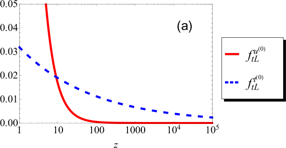
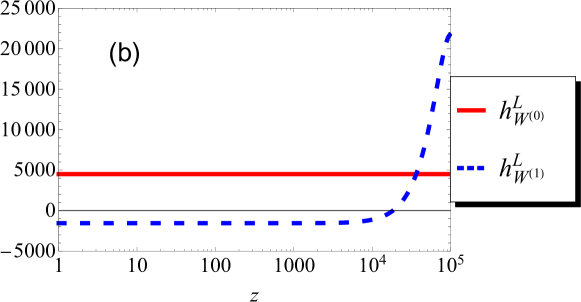
Figure 1: Behavior of dominant component of the wave functions for fermions and $W^{(n)}$ bosons for $N_{F}=4$, $z_{L}=10^{5}$ ($\theta_{H}=0.115$). (a) Red-solid and blue-dashed lines are $f_{tL}^{t^{(0)}}$ for the top and $f_{tL}^{u^{(0)}}$ for the up quark, respectively. (b) Red-solid and blue-dashed lines are $h^{L}_{W^{(0)}}$ for $W^{(0)}$ and $h^{L}_{W^{(1)}}$ for $W^{(1)}$ bosons, respectively.

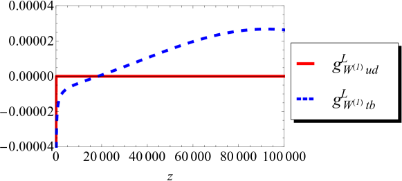
Figure 2: Integrand of the coupling $g_{W^{(1)}UD}^{L}$ in (D.4). Red-solid and blue-dashed lines are for $(U,D)=(t,b)$ and $(u,d)$, respectively.

In Table 5, $HWW^{\prime}$ ($W^{\prime}=W^{(n)},W_{R}^{(n)}$) and $HZZ^{\prime}$ ($Z^{\prime}=Z^{(n)},Z_{R}^{(n)}$) couplings are tabulated. We note that $H\gamma^{(n)}Z^{(m)}$ and $H\gamma^{(n)}Z_{R}^{(m)}$ couplings vanish. We find that $g_{WWH}$ and $g_{ZZH}$ couplings are given by the SM values multiplied by $\cos\theta_{H}$. $g_{W^{(1)}WH}$ and $g_{W_{R}^{(1)}WH}$ are a few times larger than $g_{WWH}$, and similar relations holds among $g_{Z_{R}^{(1)}ZH}$, $g_{Z^{(1)}ZH}$ and $g_{ZZH}$. All $g_{W^{\prime(n)}WH}$ and $g_{Z^{\prime}(n)ZH}$ couplings become small as $n$ becomes larger.

Table 5: Couplings of $W^{(n)}$, $Z^{(n)}$, $\gamma^{(n)}$ and $Z_{R}^{(n)}$ to $WH$, $ZH$ in the unit of GeV.

$N_{F}=4$, $z_{L}=10^{5}$ ($\theta_{H}=0.115$)
	$n=0$	$1$	$2$	$3$	$4$
$g_{W^{(n)}WH}/(g_{w}\cos\theta_{H})$	80.0	255	2.57	45.4	0.220
$g_{Z^{(n)}ZH}/(g_{w}\cos\theta_{H}/\cos\theta_{W})$	91.2	291	3.35	51.8	0.286
$g_{W_{R}^{(n)}WH}/g_{w}$	—	266	50.5	20.6	11.1
$g_{Z_{R}^{(n)}ZH}/(g_{w}/\cos\theta_{W})$	—	223	42.3	17.2	9.27

$N_{F}=4$ $z_{L}=10^{4}$ ($\theta_{H}=0.0737$)
	$n=0$	$1$	$2$	$3$	$4$
$g_{W^{(n)}WH}/(g_{w}\cos\theta_{H})$	80.0	225	1.89	39.2	0.169
$g_{Z^{(n)}ZH}/(g_{w}\cos\theta_{H}/\cos\theta_{W})$	91.2	257	2.46	44.8	0.220
$g_{W_{R}^{(n)}WH}/g_{w}$	—	238	45.1	18.4	9.89
$g_{Z_{R}^{(n)}ZH}/(g_{w}/\cos\theta_{W})$	—	199	37.7	15.4	8.27

In Table 6, trilinear vector-boson couplings are tabulated. The $g_{WWZ}$ coupling is very close to its SM value $g_{w}\cos\theta_{W}$. The deviation is one part in $10^{8}$. $g_{\gamma WW}$ is exactly $e$, which reflects the unbroken $U(1)_{\rm em}$ gauge symmetry. Couplings among the first KK and two SM vector bosons are suppressed by a factor of ${\cal O}(10^{-4})$, which is close to the square of the ratio of the weak boson mass to the 1st KK boson mass.

Table 6: Trilinear vector-boson couplings of $W^{(n)}$, $Z^{(n)}$, $\gamma^{(n)}$ and $Z_{R}^{(n)}$ to $W^{+}W^{-}$, $WZ$

$N_{F}=4$, $z_{L}=10^{5}$ ($\theta_{H}=0.115$)
	$n=0$	$1$	$2$	$3$	$4$
$g_{W^{(n)}WZ}/(g_{w}\cos\theta_{W})$	0.9999998	$-7.35\times 10^{-4}$	$-9.63\times 10^{-7}$	$-2.64\times 10^{-5}$	$-1.60\times 10^{-7}$
$g_{Z^{(n)}WW}/(g_{w}\cos\theta_{W})$	0.9999998	$-3.96\times 10^{-4}$	$1.62\times 10^{-8}$	$-1.42\times 10^{-5}$	$-1.17\times 10^{-7}$
$g_{\gamma^{(n)}WW}/e$	1	$-1.13\times 10^{-3}$	$-4.04\times 10^{-5}$	$-7.63\times 10^{-6}$	$-2.07\times 10^{-6}$
$g_{Z_{R}^{(n)}WW}/g_{w}$	—	$5.51\times 10^{-4}$	$1.99\times 10^{-5}$	$3.28\times 10^{-6}$	$9.53\times 10^{-7}$
$g_{W_{R}^{(n)}WZ}/g_{w}$	—	$7.51\times 10^{-4}$	$2.71\times 10^{-5}$	$4.47\times 10^{-6}$	$1.30\times 10^{-6}$

$N_{F}=4$, $z_{L}=10^{4}$ ($\theta_{H}=0.0737$)
	$n=0$	$1$	$2$	$3$	$4$
$g_{W^{(n)}WZ}/(g_{w}\cos\theta_{W})$	0.99999995	$-3.32\times 10^{-4}$	$-3.88\times 10^{-7}$	$-1.15\times 10^{-5}$	$-6.04\times 10^{-8}$
$g_{Z^{(n)}WW}/(g_{w}\cos\theta_{W})$	0.99999995	$-1.73\times 10^{-4}$	$-1.46\times 10^{-8}$	$-6.18\times 10^{-6}$	$-4.43\times 10^{-8}$
$g_{\gamma^{(n)}WW}/e$	1	$-4.95\times 10^{-4}$	$-1.76\times 10^{-5}$	$-3.46\times 10^{-6}$	$-9.22\times 10^{-7}$
$g_{Z_{R}^{(n)}WW}/g_{w}$	—	$2.53\times 10^{-4}$	$9.10\times 10^{-6}$	$1.51\times 10^{-6}$	$4.37\times 10^{-7}$
$g_{W_{R}^{(n)}WZ}/g_{w}$	—	$3.45\times 10^{-4}$	$1.24\times 10^{-5}$	$2.05\times 10^{-6}$	$5.96\times 10^{-7}$

5.2 Decay width

In Tables 7 and 8, decay widths of $W$ and $W_{R}$ boson are tabulated, respectively. Since the $W^{(1)}$ boson couples equally to the light SM fermions except for $b$ and $t$ quarks, partial decay widths to light SM fermions are almost identical besides the QCD color factor. The $W^{(1)}$ coupling to $t$ and $b$ quarks is larger than the couplings to other fermion pairs. The $W^{(1)}$ decay to $tb$ dominates over decay to other fermion pairs. Partial decay widths of $W^{(1)}$ to $WZ$ and $WH$ are almost identical:

$$\Gamma(W^{(1)}\to WH) \simeq \Gamma(W^{(1)}\to WZ),\quad\therefore\eta_{W^{(1)}}\simeq 1,$$

$$\Gamma(W_{R}^{(1)}\to WH) \simeq \Gamma(W_{R}^{(1)}\to WZ),\quad\therefore\eta_{W_{R}^{(1)}}\simeq 1.$$ (5.1)

We also find

$$\Gamma(W^{(1)}\to WH)\sim\Gamma(W_{R}^{(1)}\to WH),\quad\Gamma(W^{(1)}\to WZ)\sim\Gamma(W_{R}^{(1)}\to WZ).$$ (5.2)

Since the $W_{R}^{(n)}$ boson does not couple to SM fermions, and $W_{R}^{(1)}$ decay only to the SM bosons.

In Tables 9, 10 and 11, decay widths of $Z^{(1)}$, $\gamma^{(1)}$ and $Z_{R}^{(1)}$ are tabulated, respectively. Compared with $W^{(1)}$ and $W_{R}^{(1)}$, $\gamma^{(1)}$ and $Z_{R}^{(1)}$ have large total widths

$$\Gamma_{\gamma^{(1)}}/M_{\gamma^{(1)}} = \begin{cases}0.151&\text{ for $N_{F}=4$, $z_{L}=10^{5}$ ($\theta_{H}=0.115$)}\\ 0.125&\text{ for $N_{F}=4$, $z_{L}=10^{4}$ ($\theta_{H}=0.0737$)}\end{cases}$$ (5.3)

$$\Gamma_{Z_{R}^{(1)}}/M_{Z_{R}^{(1)}} = \begin{cases}0.129&\text{ for $N_{F}=4$, $z_{L}=10^{5}$ ($\theta_{H}=0.115$)}\\ 0.133&\text{ for $N_{F}=4$, $z_{L}=10^{4}$ ($\theta_{H}=0.0737$)}.\end{cases}$$ (5.4)

From the tables, one finds that

$$\Gamma(Z^{(1)}\to HZ) \simeq \sum_{Z^{\prime}=Z^{(1)},\gamma^{(1)}}\Gamma(Z^{\prime}\to W^{+}W^{-}),$$ (5.5)

$$\Gamma(Z_{R}^{(1)}\to HZ) \simeq \Gamma(Z_{R}^{(1)}\to W^{+}W^{-}).$$ (5.6)

$\gamma^{(1)}$ and $Z^{(1)}$ are almost degenerate. The relation (5.5) follows from the relation among Higgs-vector boson and trilinear vector boson couplings

$$\frac{g_{\gamma^{(1)}ZH}^{2}+g_{Z^{(1)}ZH}^{2}}{M_{Z}^{2}} \simeq (g_{\gamma^{(1)}WW}^{2}+g_{Z^{(1)}WW}^{2})\frac{M_{Z^{\prime}}^{4}}{M_{Z}^{4}},$$ (5.7)

where $M_{\gamma^{(1)}}\simeq M_{Z^{(1)}}\equiv M_{Z^{\prime}}$ and $g_{\gamma^{(1)}ZH}=0$.

Table 7: Partial and total decay width of $W^{-(1)}$ in the unit of GeV.

$N_{F}=4$, $z_{L}=10^{5}$ ($\theta_{H}=0.115$)
mode	$e^{-}\bar{\nu}_{e}$	$\mu^{-}\bar{\nu}_{\mu}$	$\tau^{-}\bar{\nu}_{\tau}$	$d\bar{u}$	$s\bar{c}$	$b\bar{t}$	$W^{-}Z$	$W^{-}H$	total
$\Gamma$	2.00	2.00	1.99	5.99	5.98	84.7	42.7	42.1	187

$N_{F}=4$, $z_{L}=10^{4}$ ($\theta_{H}=0.0737$)
mode	$e^{-}\bar{\nu}_{e}$	$\mu^{-}\bar{\nu}_{\mu}$	$\tau^{-}\bar{\nu}_{\tau}$	$d\bar{u}$	$s\bar{c}$	$b\bar{t}$	$W^{-}Z$	$W^{-}H$	total
$\Gamma$	3.63	3.63	3.62	10.88	10.88	219	46.9	47.2	346

Table 8: Partial and total decay widths of $W_{R}^{-(1)}$ in the unit of GeV.

$N_{F}=4$, $z_{L}=10^{5}$ ($\theta_{H}=0.115$)
SM fermions	$W^{-}Z$	$W^{-}H$	total
0	43.4	43.4	86.8

$N_{F}=4$, $z_{L}=10^{4}$ ($\theta_{H}=0.0737$)
SM fermions	$W^{-}Z$	$W^{-}H$	total
0	48.7	48.8	97.4

Table 9: Partial and total decay widths of $Z^{(1)}$ in the unit of GeV.

$N_{F}=4$, $z_{L}=10^{5}$ ($\theta_{H}=0.115$)
$e^{+}e^{-}$	$\mu^{+}\mu^{-}$	$\tau^{+}\tau^{-}$	$\nu_{e}\bar{\nu}_{e}$	$\nu_{\mu}\bar{\nu}_{\mu}$	$\nu_{\tau}\bar{\nu}_{\tau}$	$u\bar{u}$	$c\bar{c}$	$t\bar{t}$	$d\bar{d}$	$s\bar{s}$	$b\bar{b}$	$W^{+}W^{-}$	$ZH$	total
40.4	35.7	32.1	1.30	1.30	1.30	53.3	46.1	48.5	15.7	13.8	45.7	16.1	54.8	406

$N_{F}=4$, $z_{L}=10^{4}$ ($\theta_{H}=0.0737$)
$e^{+}e^{-}$ $\mu^{+}\mu^{-}$ $\tau^{+}\tau^{-}$ $\nu_{e}\bar{\nu}_{e}$ $\nu_{\mu}\bar{\nu}_{\mu}$ $\nu_{\tau}\bar{\nu}_{\tau}$ $u\bar{u}$ $c\bar{c}$ $t\bar{t}$ $d\bar{d}$ $s\bar{s}$ $b\bar{b}$ $W^{+}W^{-}$ $ZH$ total 48.1 42.5 38.0 2.36 2.36 2.36 64.4 55.5 84.4 20.3 18.1 106.8 17.8 61.1 564

Table 10: Partial and total decay width of $\gamma^{(1)}$ in the unit of GeV.

$N_{F}=4$, $z_{L}=10^{5}$ ($\theta_{H}=0.115$)
$e^{+}e^{-}$	$\mu^{+}\mu^{-}$	$\tau^{+}\tau^{-}$	$\nu_{e}\bar{\nu}_{e}$	$\nu_{\mu}\bar{\nu}_{\mu}$	$\nu_{\tau}\bar{\nu}_{\tau}$	$u\bar{u}$	$c\bar{c}$	$t\bar{t}$	$d\bar{d}$	$s\bar{s}$	$b\bar{b}$	$W^{+}W^{-}$	$ZH$	total
133.0	117.4	105.7	0	0	0	171.0	147.2	93.0	42.8	36.8	23.3	39.3	0	909

$N_{F}=4$, $z_{L}=10^{4}$ ($\theta_{H}=0.0737$)
$e^{+}e^{-}$	$\mu^{+}\mu^{-}$	$\tau^{+}\tau^{-}$	$\nu_{e}\bar{\nu}_{e}$	$\nu_{\mu}\bar{\nu}_{\mu}$	$\nu_{\tau}\bar{\nu}_{\tau}$	$u\bar{u}$	$c\bar{c}$	$t\bar{t}$	$d\bar{d}$	$s\bar{s}$	$b\bar{b}$	$W^{+}W^{-}$	$ZH$	total
158.9	140.2	125.2	0	0	0	204.6	175.0	101.0	51.1	43.8	25.3	43.6	0	1068

Table 11: Partial and total decay widths of $Z_{R}^{(1)}$ in the unit of GeV.

$N_{F}=4$, $z_{L}=10^{5}$ ($\theta_{H}=0.115$)
$e^{+}e^{-}$	$\mu^{+}\mu^{-}$	$\tau^{+}\tau^{-}$	$\nu_{e}\bar{\nu}_{e}$	$\nu_{\mu}\bar{\nu}_{\mu}$	$\nu_{\tau}\bar{\nu}_{\tau}$
71.3	63.8	58.0	${\cal O}(10^{-16})$	${\cal O}(10^{-11})$	${\cal O}(10^{-7})$
$u\bar{u}$	$c\bar{c}$	$t\bar{t}$	$d\bar{d}$	$s\bar{s}$	$b\bar{b}$
92.0	80.4	146.2	23.0	20.1	111.9
$W^{+}W^{-}$	$ZH$				total
30.5	30.7				729

$N_{F}=4$, $z_{L}=10^{4}$ ($\theta_{H}=0.0737$)
$e^{+}e^{-}$	$\mu^{+}\mu^{-}$	$\tau^{+}\tau^{-}$	$\nu_{e}\bar{\nu}_{e}$	$\nu_{\mu}\bar{\nu}_{\mu}$	$\nu_{\tau}\bar{\nu}_{\tau}$
83.9	75.2	68.1	${\cal O}(10^{-13})$	${\cal O}(10^{-10})$	${\cal O}(10^{-6})$
$u\bar{u}$	$c\bar{c}$	$t\bar{t}$	$d\bar{d}$	$s\bar{s}$	$b\bar{b}$
108.5	94.6	268.4	27.1	23.7	240.3
$W^{+}W^{-}$	$ZH$				total
34.1	34.3				1058

6 Cross section

In this section we evaluate cross sections in $pp$-collisions for various final states. In the numerical evaluation we use CTEQ5 parton distribution functions Lai:1999wy .

6.1 $W^{\prime}\to tb$, $\mu\nu$ and $Z^{\prime}\to\ell^{+}\ell^{-}$

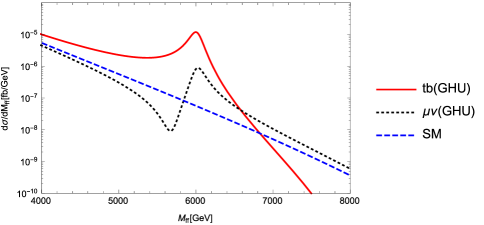
Figure 3: $pp(d\bar{u})\to\{W^{-},\,W^{(1)-}\}\to b\bar{t},\mu^{-}\bar{\nu}_{\mu}$ differential cross sections $d\sigma/dM_{\rm ff}$ at $\sqrt{s_{pp}}=14$ TeV for $N_{F}=4$, $z_{L}=10^{5}$ ($\theta_{H}=0.115$). $M_{\rm ff}$ is the invariant mass of $(b,\bar{t})$ or $(\mu,\bar{\nu})$. Red-solid, black-dotted lines are for the $b\bar{t}$ and $\mu^{-}\bar{\nu}$ final states in GHU. Blue-dashed line is the cross section in the SM. Cross sections for the processes $pp\to W^{(1)-}\to f\bar{f}^{\prime}$, $(f,f^{\prime})=(e^{-},\nu_{e}),(\tau^{-},\nu_{\tau})$ are almost identical with that of $\mu^{-}\bar{\nu}$, whereas cross section for $(f,f^{\prime})=(d,u),(s,c)$ final states is three times as large as that of $\mu^{-}\bar{\nu}$ due to the color factor.

In Figure 3, the differential cross sections of processes $pp\to\{W^{-},\,W^{(1)-}\}\to b\bar{t},\mu^{-}\bar{\nu}$ are plotted. For light fermion doublet paris $\ell\bar{\nu},d\bar{u},s\bar{c}$ in the final state, due to the flipped-signs of the couplings to $W^{(1)}$, a clear deficit of cross section just below the resonance $M_{\mu\nu}\sim M_{W^{(1)}}$ is observed. For processes with $b\bar{t}$ final state, a deficit of cross section is observed above the resonance $M_{tb}>M_{W^{(1)}}$, since the $W^{(1)}\bar{t}b$ coupling has opposite sign relative to the $W^{(1)}\bar{u}d$ coupling.

When the final state contains a neutrino, the transverse momentum distribution $d\sigma/dp_{T}$ with respect to the transverse momentum of charged lepton, $p_{T}$, gives information on the mass of $W^{\prime}$. The transverse-momentum distribution at parton-level is given in Appendix G. The $p_{T}$ distribution in $pp$ collision is given by

$$\frac{d\sigma(pp\to e^{-}\bar{\nu}+X)}{dp_{T}}(p_{T}) = \int_{0}^{1}d\tau\biggl{\{}\frac{dp_{T}(d\bar{u}\to e^{-}\bar{\nu})}{dp_{T}}(s_{pp}\tau,p_{T})\cdot\frac{dL_{d\bar{u}}}{d\tau}(\tau)\biggl{\}},$$ (6.1)

where the parton luminosity $dL_{d\bar{u}}/d\tau$ is given in terms of parton distribution functions $f_{q}(x_{1},Q)$ by

$$\frac{dL_{d\bar{u}}}{d\tau}(\tau) = \int_{0}^{1}dx_{1}\int_{0}^{1}dx_{2}[f_{d}(x_{1},Q)f_{\bar{u}}(x_{2},Q)+f_{d}(x_{2},Q)f_{\bar{u}}(x_{1},Q)]\delta(\tau-x_{1}x_{2}),$$

$$Q = s_{pp}\tau.$$ (6.2)

In Figure 4 the $p_{T}$-distribution $d\sigma(pp\to e^{-}\bar{\nu})/dp_{T}$ is plotted. In the figure, Jacobian peak at $p_{T}=M_{M^{(1)}}/2\simeq 3\,\text{TeV}$ is observed.

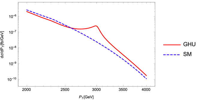
Figure 4: $d\sigma(pp\to e^{-}\bar{\nu}_{e})/dp_{T}$ as a function of $p_{T}$ at $\sqrt{s_{pp}}=14\,\text{TeV}$ for $N_{F}=4$, $z_{L}=10^{5}$ ($\theta_{H}=0.115$). Red-solid and blue-dashed lines are for the GHU model and the SM, respectively.

For the process $pp(u\bar{u},d\bar{d})\to Z^{\prime}\to\ell^{+}\ell^{-}$, we show the plot of the differential cross section $d\sigma/dM_{\mu\mu}$ in Figure 5. In the plot the updated decay widths of $Z^{\prime}$ ($Z^{\prime}=\gamma^{(1)}$, $Z^{(1)}$ and $Z_{R}^{(1)}$) has been used, which takes bosonic final states ($W^{+}W^{-}$ and $ZH$) into account, and is ${\cal O}(10\%)$ bigger than that used in the previous paper Funatsu:2014fda . We stress that the rate of $Z^{\prime}$ production is rather large, and it is promising to see the $Z^{\prime}$ events at the current LHC Run 2. Since in this model $Z^{\prime}$ bosons have large widths, at the early stage of LHC experiment, sporadic events of high-energy $\mu^{+}\mu^{-}$ final states will be seen. For $\theta_{H}=0.115$ ($M_{Z^{(1)},\gamma^{(1)}}\sim 6.0\,\text{TeV}$, $M_{Z_{R}^{(1)}}\sim 5.7\,\text{TeV}$), with the 30 fb^-1 and $\sqrt{s_{pp}}=13\,\text{TeV}$ data, expected numbers of events in GHU $N_{GHU}$ and SM signal $N_{SM}$, and significance $S$ are $N_{GHU}/N_{SM}(S)=8.4/3.6\,(2.2)$, $3.9/0.26\,(3.7)$, $2.6/0.02\,(4.4)$, $2.9/0.004\,(6.0)$, $0.65/0.0002\,(3.0)$ and $0.01/1\times 10^{-5}\,(0.34)$ for bins (GeV) $[2000,3000]$, $[3000,4000]$, $[4000,5000]$, $[5000,6000]$, $[6000,7000]$ and $[7000,8000]$, respectively. In this case, an excess of high-energy ($M_{\mu\mu}\gtrsim 3000\,\text{GeV}$) events is expected. For smaller $\theta_{H}$ (heavier $M_{Z^{\prime}}$), the signals becomes smaller and more data is required for confirming/rejecting the model. For $\theta_{H}=0.0737$ ($M_{Z^{(1)},\gamma^{(1)}}\sim 8.5\,\text{TeV}$, $M_{Z_{R}^{(1)}}\sim 7.9\,\text{TeV}$), with the 1000 fb^-1 and $\sqrt{s_{pp}}=14\,\text{TeV}$ data, $N_{GHU}/N_{SM}(S)=140/155\,(1.21)$, $23/12\,(2.7)$, $8.5/1.3\,\,(4.2)$, $3.7/0.14\,(4.12)$, $0.7/0.006\,(2.3)$ and $0.3/0.0004\,(1.7)$ for bins (GeV) $[2000,3000]$, $[3000,4000]$, $[4000,5000]$, $[5000,6000]$, $[6000,7000]$ and $[7000,8000]$, respectively.

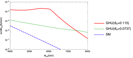
Figure 5: Differential cross section $d\sigma/dM_{\mu\mu}$ of the process $pp(u\bar{u},d\bar{d})\to\{\gamma,\,Z,\,Z^{(1)},\,\gamma^{(1)},\,Z_{R}^{(1)}\}\to\mu^{+}\mu^{-}$ at $\sqrt{s}=14$ TeV. $M_{\mu\mu}$ is the invariant mass of $\mu^{+}\mu^{-}$. Solid [red], dotted [green] and dashed [blue] lines are the $Z^{\prime}$ resonance in the GHU for $N_{F}=4$, $z_{L}=10^{5}$ ($\theta_{H}=0.115$), $N_{F}=4$, $z_{L}=10^{4}$ ($\theta_{H}=0.0737$) and the SM, respectively. The cross section for the $e^{+}e^{-}$ final state is identical to the $\mu^{+}\mu^{-}$ final state.

6.2 $W^{\prime}\to WH$ and $Z^{\prime}\to ZH$

In Figures 6 and 7, differential cross sections of processes $pp\to\{W^{-},\,W^{(1)-}\}\to W^{-}H$ and $pp\to\{Z,Z^{(1)},Z_{R}^{(1)}\}\to ZH$ are plotted, respectively. Compared with the $WH$ mode, cross section for $ZH$ mode is bigger and the width is wider. It is due to the fact that $Z^{(1)}$ and $Z_{R}^{(1)}$ have large couplings to the right-handed quarks, and their widths are large.

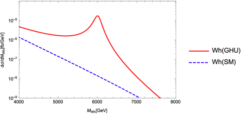
Figure 6: Differential cross section $d\sigma/M_{Wh}$ of the process $pp(d\bar{u})\to\{W^{-},\,W^{(1)-}\}\to W^{-}H$ at $\sqrt{s_{pp}}=14$ TeV for $N_{F}=4$, $z_{L}=10^{5}$ ($\theta_{H}=0.115$). $M_{Wh}$ is the invariant mass of $WH$. Red-solid and blue-dashed lines show cross sections in GHU and in the SM, respectively.

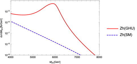
Figure 7: Differential cross section $d\sigma/dM_{Zh}$ of the process $pp(u\bar{u},d\bar{d})\to\{Z,\,Z^{(1)},\,Z_{R}^{(1)}\}\to ZH$ cross section at $\sqrt{s_{pp}}=14$ TeV for $N_{F}=4$, $z_{L}=10^{5}$ ($\theta_{H}=0.115$). $M_{Zh}$ is the invariant mass of $ZH$. Red-solid and blue-dashed lines show cross sections in GHU and in the SM, respectively.

6.3 $W^{\prime}\to WZ$ and $Z^{\prime}\to WW$

In Figures 8 and 9, differential cross sections of the processes $pp\to\{\gamma,\,Z,\,Z^{(1)},\,\gamma^{(1)},\,Z_{R}^{(1)}\}\to W^{+}W^{-}$ and $pp\to\{W^{-},\,W^{(1)-}\}\to W^{-}Z$ are plotted, respectively. For the $WZ$ final states, the signal of the resonance of $W^{\prime}$ is a few times larger than that of the SM. For the $WW$ final states, the contribution from $Z^{\prime}$ resonances is much smaller than the SM cross section so that the signal is hard to see.

We comment that there are no $s$-channel processes with $ZZ$ final states mediated by vector bosons. The process mediated by KK gravitons Davoudiasl:1999jd ; Davoudiasl:2000wi can be ignored, as the couplings of KK gravitons to the SM fields are suppressed by $k/M_{Pl}\ll 1$, where $M_{Pl}$ is the Planck mass.

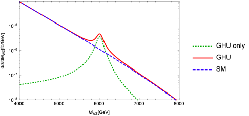
Figure 8: Differential cross section $d\sigma/dM_{WZ}$ of the process $pp(d\bar{u})\to\{W^{-},W^{(1)-}\}\to W^{-}Z$ at $\sqrt{s_{pp}}=14$ TeV for $N_{F}=4$, $z_{L}=10^{5}$ ($\theta_{H}=0.115$). $M_{\rm WZ}$ is the invariant mass of $WZ$. Green-dotted line shows the $s$-channel $W^{\prime}$ signals in GHU model. Blue-dashed line shows the SM prediction including $s$-, $t$- and $u$-channels Brown:1979ux . Red-solid line is the sum of SM and GHU signals.

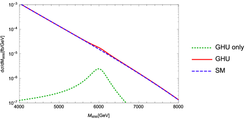
Figure 9: Differential cross section $d\sigma/dM_{WW}$ of the process $pp(u\bar{u},d\bar{d})\to\{\gamma,\,Z,\,Z^{(1)},\,\gamma^{(1)},\,Z_{R}^{(1)}\}\to W^{+}W^{-}$ at $\sqrt{s_{pp}}=14$ TeV for $N_{F}=4$, $z_{L}=10^{5}$ ($\theta_{H}=0.115$). $M_{WW}$ is the invariant mass of $W^{+}W^{-}$. Green-dotted line shows the s-channel $W^{\prime}$ signals in GHU model. Blue-dashed line shows the SM prediction including $s$-, $t$- and $u$-channels Brown:1978mq . Red-solid line is the sum of SM and GHU signals.

6.4 Unitarity in $f\bar{f}^{\prime}\to WZ$

It is important to see how the unitarity is ensured when vector bosons are involved in the final states. The unitarity in the $W$ boson scattering, $WW\to WW$ in the gauge-Higgs unification has been studied in Haba:2009hw by using position-space propagators. In the present paper we are considering $f\bar{f}\to V^{\prime}\to WW$, $WZ$. In these processes, $t$- and $u$-channel amplitudes must be included to cancel the growing part of the the $s$-channel amplitude at $\sqrt{s}\gg m_{V^{\prime}}$ (See Fig. 10).

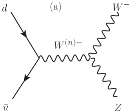
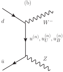
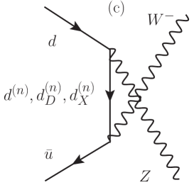
Figure 10: Diagrams of $d\bar{u}\to WZ$ at a energy scale above $M_{KK}$. (a), (b) and (c) represent $s$-, $t$- and $u$-channels, respectively. $W^{(n)}$ is the $n$-th KK state of $W$, whereas ${\cal D}^{(n)}$ and ${\cal U}^{(n)}$ are $n$-th KK states of $d$ and $u$, and partners $d_{D,X}^{(n)}$, $u_{U,B}^{(n)}$, respectively.

Let us consider the process $d(p_{1})\bar{u}(p_{2})\to W^{-}(k_{1})Z(k_{2})$. When the initial states are given by $d_{R}\overline{u_{L}}$, there are no $s$-channel contribution as $W^{(n)}$ do not couple to the right-handed quarks. For the final state bosons with longitudinal polarization, $\varepsilon^{\mu}(k_{1})\simeq k_{1}^{\mu}/M_{W}$ and $\varepsilon^{\nu}(k_{2})\simeq k_{2}^{\nu}/M_{Z}$, $t$- and $u$-channel amplitudes at very high-energy $\sqrt{s}\gg m_{KK}$ are expressed as

$${\cal M}_{t} \sim \frac{1}{M_{W}M_{Z}}\sum_{{\cal U}}g_{Wd{\cal U}}^{R}g_{Zu{\cal U}}^{R}\bar{v}(p_{2})\not{k}_{2}P_{R}\frac{(\not{p}_{1}-\not{k}_{1})}{(p_{1}-k_{1})^{2}}\not{k}_{1}P_{R}u(p_{1})$$ (6.3)

$$= \frac{1}{2M_{W}M_{Z}}\sum_{{\cal U}}g_{Wd{\cal U}}^{R}g_{Zu{\cal U}}^{R}\bar{v}(p_{2})(\not{k}_{2}-\not{k}_{1})P_{R}u(p_{1}),$$

$${\cal M}_{u} \sim \frac{1}{M_{W}M_{Z}}\sum_{{\cal D}}g_{Zd{\cal D}}^{R}g_{Wu{\cal D}}^{R}\bar{v}(p_{2})\not{k}_{1}P_{R}\frac{(\not{p}_{1}-\not{k}_{2})}{(p_{1}-k_{2})^{2}}\not{k}_{2}P_{R}u(p_{1})$$ (6.4)

$$= \frac{1}{2M_{W}M_{Z}}\sum_{{\cal D}}g_{Zd{\cal D}}^{R}g_{Wu{\cal D}}^{R}\bar{v}(p_{2})(\not{k}_{1}-\not{k}_{2})P_{R}u(p_{1}),$$

where $P_{L/R}\equiv(1\mp\gamma_{5})/2$, and ${\cal U}$ and ${\cal D}$ denote KK-excited states with $Q_{EM}=+2/3$ and $-1/3$, respectively. Here we have retained contributions only from the first KK states of fermions, as the $Wu{\cal D}^{(n)}$, $Wd{\cal U}^{(n)}$, $Zu{\cal U}^{(n)}$ and $Zd{\cal D}^{(n)}$ couplings ($n\geq 2$), etc., are all negligibly small.

In order for the growing parts of ${\cal M}_{t}$ and ${\cal M}_{u}$ to cancel with each other, the relation

$$\sum_{{\cal U}}g_{W{\cal U}d}^{R}g_{Zu{\cal U}}^{R} \simeq \sum_{{\cal D}}g_{Z{\cal D}d}^{R}g_{Wu{\cal D}}^{R}$$ (6.5)

should be satisfied. With the values in Tables 14-18, one finds that in (6.5)

$$(\text{L.H.S}) \simeq g_{Wdu^{(1)}}^{R}g_{Zuu^{(1)}}^{R}+g_{Wdu_{B}^{(1)}}^{R}g_{Zuu_{B}^{(1)}}^{R}$$ (6.6)

$$= [(-2.95)\cdot(-0.65)+(1.29)\cdot(-1.48)]\times 10^{-4}g_{w}^{2}/\sqrt{2},$$

$$(\text{R.H.S}) \simeq g_{{dd^{(1)}}}^{R}g_{Wud^{(1)}}^{R}+g_{Zdd_{X}^{(1)}}^{R}g_{Wud_{X}^{(1)}}^{R}$$ (6.7)

$$= [(1.48)\cdot(-1.3)+(0.65)\cdot(2.95)]\times 10^{-4}g_{w}^{2}/\sqrt{2}.$$

We observe that the relation (6.5) is well satisfied. We note that

$$g_{Wdu^{(1)}}^{R}=-g_{Wud_{X}^{(1)}}^{R},\quad g_{Zuu^{(1)}}^{R}=-g_{Zd{d_{X}}^{(1)}}^{R},$$

$$g_{Wdu_{B}^{(1)}}^{R}=-g_{Wud^{(1)}}^{R},\quad g_{Zdd^{(1)}}^{R}=-g_{Zu{u_{B}}^{(1)}}^{R}.$$ (6.8)

When the initial states are given by $d_{L}\overline{u_{R}}$, there are contributions from $s$-channel amplitudes. The condition for the cancellations is given by (c.f. Chapter 21 of Peskin:1995ev )

$$\sum_{n=0}^{\infty}g_{W^{(n)}ud}^{L}\,g_{W^{(n)}WZ} \simeq \sum_{{\cal U}^{\prime}}g_{Wd{\cal U^{\prime}}}^{L}g_{Zu{\cal U}^{\prime}}^{L}-\sum_{{\cal D}^{\prime}}g_{Zd{\cal D}^{\prime}}^{L}g_{Wu{\cal D}^{\prime}}^{L},$$ (6.9)

where ${\cal U}^{\prime}$ and ${\cal D}^{\prime}$ represent all SM and non-SM fermions in the first generation with $Q_{EM}=2/3$ and $-1/3$, respectively. From Tables 14, 15, 17 and 18 in Appendix D, one finds that $Wu{\cal D}^{(n)}$, $Wd{\cal U}^{(n)}$, $Zu{\cal U}^{(n)}$ and $Zd{\cal D}^{(n)}$ couplings ($n\geq 1$) are all small. Hence the right-hand-side of (6.9) will be approximately given by

$$(\text{R.H.S.}) \simeq g_{Wdu}(g_{Zuu}-g_{Zdd})=0.877163\cdot g_{w}^{2}/\sqrt{2},$$ (6.10)

The left-hand side is approximately given, with use of Tables. 4 and 6, by

$$(\text{L.H.S.}) \simeq \sum_{n=0}^{4}g_{W^{(n)}ud}g_{W^{(n)}WZ}=0.877162\cdot g_{w}^{2}/\sqrt{2}.$$ (6.11)

It is recognized that (6.9) is also quantitatively well-satisfied.

In an analogous way one can confirm the unitarity of the amplitude of $f\bar{f}\to W^{+}W^{-}$. In this case KK bosons of $\gamma$, $Z$ and $Z_{R}$ are involved in the $s$-channel amplitudes.

7 Summary

In this paper we have studied the collider signals of $W^{\prime}$ and $Z^{\prime}$ in the $SO(5)\times U(1)_{X}$ gauge-Higgs unification.

First we evaluated the couplings of $W^{\prime}$ and $Z^{\prime}$ to the SM fields. We found that the $W^{(1)}$ couplings to light fermions and to top-bottom are different in signs, which is explained from the different behavior of wave functions of fields along the extra dimension.

Next we evaluated the decay rates of neutral and charged KK vector bosons. The total decay widths of $Z^{\prime}$ are large. $\Gamma_{Z^{\prime}}/M_{Z^{\prime}}=15\%$, $6.6\%$ and $13\%$ for $Z^{\prime}=\gamma^{(1)}$, $Z^{(1)}$ and $Z_{R}^{(1)}$, respectively. On the other hand, $W^{(1)}$ has a narrow total width: $\Gamma_{W^{(1)}}/M_{W^{(1)}}\simeq 3\%$. Several interesting relations among decay modes (5.1), (5.2), (5.5) and (5.6) are found. In the warped space $W^{(1)}$ and $W_{R}^{(1)}$ can decay to $WH$ and $WZ$. Decay width of $W^{\prime}$ to $WH$ and $WZ$ are all nearly equal with each other. For $Z^{\prime}$ it is found that $\Gamma(Z^{(1)}\to ZH)\simeq\Gamma(Z^{(1)}\to WW)+\Gamma(\gamma^{(1)}\to WW)$ and $\Gamma(Z_{R}\to ZH)\simeq\Gamma(Z_{R}\to WW)$. These properties of $W_{R}$ and $Z_{R}$ are qualitatively understood in terms of the 4D $SO(4)\times U(1)$ model introduced in Section 4.

Further we have numerically evaluated the $s$-channel cross sections of $W^{\prime}$ and $Z^{\prime}$ in the LHC. We studied not only processes with fermionic final states but also bosonic $WH$, $ZH$, $WW$ and $WZ$ final states. $W^{\prime}$ and $Z^{\prime}$ signals of GHU can be found at the LHC experiment in the processes $pp\to W^{\prime}(Z^{\prime})+X$, $W^{\prime}\to tb,WH$, and $Z^{\prime}\to e^{+}e^{-},\mu^{+}\mu^{-},ZH$ near the $W^{\prime}$ and $Z^{\prime}$ resonances. For $\theta_{H}=0.115$ ($M_{Z^{(1)},\gamma^{(1)}}\simeq 6.0\,\text{TeV}$ and $M_{Z_{R}^{(1)}}\simeq 5.7\,\text{TeV}$), with the data of 30 fb^-1, $\sqrt{s_{pp}}=13\,\text{TeV}$ at LHC, an excess of the events of $\mu^{+}\mu^{-}$ with invariant mass is expected. (e.g. expected signal[background] is $3.9$ $[0.29]$ events for the bin (GeV) $[3000,4000]$).

In the process with $WZ$ in the final state, it is found that in the amplitude the leading contributions from the longitudinal polarizations of $W$ and $Z$ in the $s$-, $t$- and $u$-channels cancel with each other so that the unitarity is preserved, provided that both KK vector bosons and KK fermions in the intermediate states are taken into account. We have confirmed numerically that this cancellation of the leading terms in the amplitude with 6 digits of precision by taking into account contributions of up to the $4$-th level of KK excited states.

We also found that the non-SM 1st KK excited state of fermions can be much lighter than other KK states. Especially the 1st KK excited top and bottom partners ($t_{U,B,T}^{(1)}$ and $b_{D,X,Y}^{(1)}$) are the lightest non-SM particles and can be singly produced in colliders. It is seen in Tables 12 and 13 that $t_{U,B,T}^{(1)}$ and $b_{D,X,Y}^{(1)}$, which are exotic partners of the top and bottom quarks respectively, have mass $M_{t_{U,B,T}^{(1)},b_{D,X,Y}^{(1)}}=4.6$ TeV ($5.4$ TeV) for $\theta_{H}=0.115$ ($0.0737$). $t_{T}^{(1)}$ and $b_{Y}^{(1)}$ have electric charges $+5/3$ and $-4/3$ and can be observed in the processes $t+W^{+}\to t_{T}\to t+W^{+}$ and $b+W^{-}\to b_{Y}\to b+W^{-}$ in colliders Contino:2008hi ; AguilarSaavedra:2009es ; Mrazek:2009yu .

The gauge-Higgs unification scenario is promising. It gives many predictions to be tested at LHC and future colliders. The 4D Higgs boson appears as the gauge boson in the extra dimension. The gauge hierarchy problem is solved. The AB phase $\theta_{H}$ is the important parameter in GHU. Many of the physical quantities are determined by $\theta_{H}$. The universal relations among $\theta_{H}$ and $m_{KK}$, Higgs cubic and quartic couplings have been found. Corrections to the decay rates for $H\to\gamma\gamma$, $Z\gamma$ due to infinitely many KK states turn out finite and small. $Z^{\prime}$ and $W^{\prime}$ are predicted around $6$ - $8$ TeV. Discovery of $Z^{\prime}$ and $W^{\prime}$ is most awaited.

Appendix A Basic formulas

A.1 $SO(5)$ generators

The $SO(5)$ generators in the spinor-representation are given by

$$T^{a_{L}}=\frac{1}{2}\begin{pmatrix}\sigma^{a}&\bm{0}\\ \bm{0}&\bm{0}\end{pmatrix},\quad T^{a_{R}}=\frac{1}{2}\begin{pmatrix}\bm{0}&\bm{0}\\ \bm{0}&\sigma^{a}\end{pmatrix},$$

$$T^{\hat{a}}=\frac{1}{2\sqrt{2}}\begin{pmatrix}&i\sigma^{a}\\ -i\sigma^{a}&\end{pmatrix},\quad T^{\hat{4}}=\begin{pmatrix}&\bm{1}\\ \bm{1}&\end{pmatrix},$$ (A.1)

and ${\mathop{\mbox{tr}}\nolimits}(T^{a}T^{b})=\frac{1}{2}\delta^{ab}$ is satisfied. Here $\sigma^{a}$ ($a=1,2,3$) are Pauli matrices. $T^{a_{L}}$ and $T^{a_{R}}$ are generators for $SU(2)_{L}$ and $SU(2)_{R}$ subgroups, respectively.

A.2 Bulk wave functions

A.2.1 Gauge boson bulk functions

Bulk functions of gauge bosons $C=C(z;\lambda)$ and $S=S(z;\lambda)$ are defined as solutions of

$$\left(\frac{d^{2}}{dz^{2}}-\frac{1}{z}\frac{d}{dz}+\lambda^{2}\right)\begin{pmatrix}C\\ S\end{pmatrix} = 0,$$ (A.2)

with boundary conditions

$$C=z_{L},\quad S=0,\quad C^{\prime}=0,\quad S^{\prime}=\lambda\quad\text{at $z=z_{L}$.}$$ (A.3)

Here $C^{\prime}\equiv(d/dz)C$ etc. The solutions are given by

$$C(z;\lambda) = +\frac{\pi}{2}\lambda zz_{L}F_{1,0}(\lambda z,\lambda z_{L}),$$

$$C^{\prime}(z;\lambda) = +\frac{\pi}{2}\lambda^{2}zz_{L}F_{0,0}(\lambda z,\lambda z_{L}),$$

$$S(z;\lambda) = -\frac{\pi}{2}\lambda zF_{1,1}(\lambda z,\lambda z_{L}),$$

$$S^{\prime}(z;\lambda) = -\frac{\pi}{2}\lambda^{2}zF_{0,1}(\lambda z,\lambda z_{L}),$$ (A.4)

where $F_{\alpha,\beta}(u,v)\equiv J_{\alpha}(u)Y_{\beta}(v)-Y_{\alpha}(u)J_{\beta}(v)$ and $J_{\alpha}(x)$ and $Y_{\alpha}(x)$ are Bessel functions of the 1st and 2nd kind, respectively. $C$, $S$ and $C^{\prime}$, $S^{\prime}$ satisfy

$$CS^{\prime}-SC^{\prime}=\lambda.$$ (A.5)

A.2.2 Fermion bulk functions

Fermion bulk functions $C_{L/R}(z;\lambda,c)$, $S_{L/R}(z;\lambda,c)$ are defined by

$$C_{L}(z;\lambda,c) = +\frac{\pi}{2}\lambda\sqrt{zz_{L}}F_{c+\frac{1}{2},c-\frac{1}{2}}(\lambda z,\,\lambda z_{L}),$$

$$S_{L}(z;\lambda,c) = -\frac{\pi}{2}\lambda\sqrt{zz_{L}}F_{c+\frac{1}{2},c+\frac{1}{2}}(\lambda z,\,\lambda z_{L}),$$

$$C_{R}(z;\lambda,c) = +\frac{\pi}{2}\lambda\sqrt{zz_{L}}F_{c-\frac{1}{2},c+\frac{1}{2}}(\lambda z,\,\lambda z_{L}),$$

$$S_{R}(z;\lambda,c) = +\frac{\pi}{2}\lambda\sqrt{zz_{L}}F_{c-\frac{1}{2},c-\frac{1}{2}}(\lambda z,\,\lambda z_{L}).$$ (A.6)

These satisfy

$$D_{+}\begin{pmatrix}C_{L}\\ S_{L}\end{pmatrix}=\lambda\begin{pmatrix}S_{R}\\ C_{R}\end{pmatrix},\quad D_{-}\begin{pmatrix}C_{R}\\ S_{R}\end{pmatrix}=\lambda\begin{pmatrix}S_{L}\\ C_{L}\end{pmatrix},$$

$$D_{\pm}(c)\equiv\pm\frac{d}{dz}+\frac{c}{z},$$

$$C_{L}C_{R}-S_{L}S_{R}=1,$$ (A.7)

and

$$C_{R}=C_{L}=1,\quad S_{R}=S_{L}=0,\quad\text{at $z=z_{L}$.}$$ (A.8)

In particular, for $c=0$ we have

$$C_{L}(z;\lambda,0) = C_{R}(z;\lambda,0)=\cos(\lambda(z-z_{L})),$$

$$S_{L}(z;\lambda,0) = -S_{R}(z;\lambda,0)=\sin(\lambda(z-z_{L})).$$ (A.9)

Appendix B Gauge boson wave functions

Wave functions for a charged vector boson $V_{C}=W^{(n)},\,W_{R}^{(m)}$ ($n=0,1,2,\cdots$, $m=1,2,\cdots$) are given by

$$\begin{pmatrix}h^{L}_{V_{C}}\\ h^{R}_{V_{C}}\\ \hat{h}_{V_{C}}\end{pmatrix} = \begin{pmatrix}v^{L}_{V_{C}}C(z;\lambda_{V_{C}})\\ v^{R}_{V_{C}}C(z;\lambda_{V_{C}})\\ \hat{v}_{V_{C}}\hat{S}(z;\lambda_{V_{C}})\end{pmatrix},$$ (B.1)

where

$$\begin{pmatrix}v^{L}_{V_{C}}\\ v^{R}_{V_{C}}\\ \hat{v}_{V_{C}}\end{pmatrix} = \frac{1}{\sqrt{r_{V_{C}}}}\begin{cases}\begin{pmatrix}\displaystyle\frac{1+c_{H}}{\sqrt{2}}\\ \displaystyle\frac{1-c_{H}}{\sqrt{2}}\\ \displaystyle-s_{H}\end{pmatrix}&V_{C}=W^{(n)}\\ \frac{\displaystyle 1}{\displaystyle\sqrt{1+c_{H}^{2}}}\begin{pmatrix}\displaystyle\frac{+1-c_{H}}{\sqrt{2}}\\ \displaystyle\frac{-1-c_{H}}{\sqrt{2}}\\ 0\end{pmatrix}&V_{C}=W_{R}^{(m)}\end{cases}$$ (B.2)

with $C=C(z;\lambda_{V_{C}})$ etc. $c_{H},s_{H}\equiv\cos\theta_{H},\sin\theta_{H}$. We have defined

$$\hat{S}(z;\lambda)\equiv\frac{C(1;\lambda)}{S(1;\lambda)}S(z;\lambda).$$ (B.3)

The mass spectrum $\{m_{V_{C}}=k\lambda_{V_{C}}\}$ is determined by

$$2SC^{\prime}(1,\lambda_{W^{(n)}})+\lambda_{W^{(n)}}s_{H}^{2} = 0,$$

$$C(1;\lambda_{W_{R}^{(m)}}) = 0,$$ (B.4)

and normalization factors are given by

$$r_{W_{R}^{(m)}} = \int_{1}^{z_{L}}\frac{dz}{kz}C(z;\lambda_{W_{R}^{(m)}})^{2},$$

$$r_{W^{(n)}} = \int_{1}^{z_{L}}\frac{dz}{kz}\bigl{\{}(1+c_{H}^{2})C(z;\lambda_{W^{(n)}})^{2}+s_{H}^{2}\hat{S}(z;\lambda_{W^{(n)}})^{2}\bigr{\}}.$$ (B.5)

Wave functions for the photon $\gamma=\gamma^{(0)}$ is given by

$$\begin{pmatrix}h^{L}_{\gamma^{(0)}}\\ h^{R}_{\gamma^{(0)}}\\ h^{B}_{\gamma^{(0)}}\end{pmatrix} = \frac{1}{\sqrt{(1+s_{\phi}^{2})L}}\begin{pmatrix}s_{\phi}\\ s_{\phi}\\ c_{\phi}\end{pmatrix},\quad\hat{h}_{\gamma^{(0)}}=0,$$ (B.6)

where $s_{\phi}\equiv\sin\phi$ and $c_{\phi}\equiv\cos\phi$. Wave functions for a massive neutral vector boson $V=Z^{(n)}$, $\gamma^{(m)}$ and $Z_{R}^{(m)}$ ($n=0,1,2,\cdots$, $m=1,2,\cdots$) are given by

$$\begin{pmatrix}h_{V}^{L}\\ h_{V}^{R}\\ \hat{h}_{V}\\ h_{V}^{B}\end{pmatrix}=\begin{pmatrix}v_{V}^{L}C(z;\lambda_{V})\\ v_{V}^{R}C(z;\lambda_{V})\\ \hat{v}_{V}\hat{S}(z;\lambda_{V})\\ v_{V}^{B}C(z;\lambda_{V})\end{pmatrix},\quad$$ (B.7)

where

$$\begin{pmatrix}v_{V}^{L}\\ v_{V}^{R}\\ \hat{v}_{V}\\ v_{V}^{B}\end{pmatrix} = \frac{1}{\sqrt{r_{V}}}\begin{cases}\displaystyle\frac{1}{\displaystyle\sqrt{1+s_{\phi}^{2}}}\begin{pmatrix}\displaystyle\frac{(1+s_{\phi}^{2})(1+c_{H})-2s_{\phi}^{2}}{\sqrt{2}}\\ \displaystyle\frac{(1+s_{\phi}^{2})(1-c_{H})-2s_{\phi}^{2}}{\sqrt{2}}\\ -(1+s_{\phi}^{2})s_{H}\\ -\sqrt{2}s_{\phi}c_{\phi}\end{pmatrix}&V=Z^{(n)}\\ \displaystyle\frac{1}{\displaystyle\sqrt{1+s_{\phi}^{2}}}\begin{pmatrix}s_{\phi}\\ s_{\phi}\\ 0\\ c_{\phi}\end{pmatrix}&V=\gamma^{(m)},\\ \displaystyle\frac{1}{\displaystyle\sqrt{1+(1+2t_{\phi}^{2})c_{H}^{2}}}\begin{pmatrix}\displaystyle\frac{+1-c_{H}}{\sqrt{2}}\\ \displaystyle\frac{-1-c_{H}}{\sqrt{2}}\\ 0\\ \sqrt{2}t_{\phi}c_{H}\end{pmatrix}&V=Z_{R}^{(m)},\end{cases}$$ (B.8)

where $t_{\phi}=\tan\phi$. The mass spectrum $\{m_{V}=k\lambda_{V}\}$ is determined by

$$C^{\prime}(1;\lambda_{\gamma^{(m)}}) = 0,$$

$$2SC^{\prime}(1;\lambda_{Z^{(n)}})+(1+s_{\phi}^{2})\lambda_{Z^{(n)}}\sin^{2}\theta_{H} = 0,$$

$$C(1;\lambda_{Z_{R}^{(m)}}) = 0,$$ (B.9)

and normalization factors are given by $r_{V}=\int_{1}^{z_{L}}\frac{dz}{kz}{\cal F}_{V}$ where

$${\cal F}_{V} = \begin{cases}C(z;\lambda_{V})^{2}&V=Z_{R}^{(m)},\,\gamma^{(m)},\\ \displaystyle\begin{matrix}c_{\phi}^{2}C(z;\lambda_{V})^{2}+(1+s_{\phi}^{2})[c_{H}^{2}C(z;\lambda_{V})^{2}+s_{H}^{2}\hat{S}(z;\lambda_{V})^{2}]\end{matrix}&V=Z^{(n)}.\end{cases}$$ (B.10)

Appendix C Masses and wave functions of $SO(5)$-vector fermions

C.1 Quark sector

C.1.1 $Q_{\rm em}=+5/3$ quark partners $(t_{T})$

$(T^{3_{L}},T^{3_{R}})=(+\frac{1}{2},+\frac{1}{2})$ of $\Psi_{1}^{q,{g}=3}$ state has an expansion

$$T(x,z) = \sqrt{k}z^{2}\sum_{n=1}^{\infty}\biggl{\{}t_{T,L}^{(n)}(x)\frac{1}{\sqrt{r_{t_{T,L}^{(n)}}}}C_{L}(z,\lambda_{t_{T}^{(n)}},c_{1})+t_{T,R}^{(n)}(x)\frac{1}{\sqrt{r_{t_{T,R}^{(n)}}}}S_{R}(z,\lambda_{t_{T}^{(n)}},c_{1})\biggr{\}},$$

where $\lambda_{t_{T}^{(n)}}=m_{t_{T}^{(n)}}/k$. The KK mass $m_{t_{T}^{(n)}}$ is determined by

$$C_{L}(1,\lambda_{t_{T}^{(n)}},c_{1}) = 0.$$ (C.2)

Normalization factors $r_{t_{T,L/R}^{(n)}}$ are determined so that they satisfy

$$\frac{1}{r_{t_{T,L}^{(n)}}}\int_{1}^{z_{L}}C_{L}(z,\lambda_{T}^{(n)},c_{1})^{2}dz=\frac{1}{r_{t_{T,R}^{(n)}}}\int_{1}^{z_{L}}S_{R}(z,\lambda_{T}^{(n)},c_{1})^{2}dz=1,$$ (C.3)

and one finds $r_{t_{T,L}^{(n)}}=r_{t_{T,R}^{(n)}}$.

C.1.2 $Q_{\rm em}=-4/3$ quark partners $(b_{Y})$

$(T^{3_{L}},T^{3_{R}})=(-\frac{1}{2},-\frac{1}{2})$ of $\Psi_{2}^{q,{g}=3}$ state has an expansion

$$Y(x,z) = \sqrt{k}z^{2}\sum_{n=1}^{\infty}\biggl{\{}b_{Y,L}^{(n)}(x)\frac{1}{\sqrt{r_{b_{Y,L}^{(n)}}}}C_{L}(z,\lambda_{b_{Y}^{(n)}},c_{2})+b_{Y,R}^{(n)}(x)\frac{1}{\sqrt{r_{b_{Y,R}^{(n)}}}}S_{R}(z,\lambda_{b_{Y}^{(n)}},c_{2})\biggr{\}},$$

where $\lambda_{b_{Y}^{(n)}}=m_{b_{Y}^{(n)}}/k$ and $m_{b_{Y}^{(n)}}$ is the KK mass, which is determined by

$$C_{L}(1,\lambda_{b_{Y}^{(n)}},c_{2}) = 0.$$ (C.5)

Factors $r_{b_{Y,L/R}^{(n)}}$ are normalized so that they satisfy

$$\frac{1}{r_{b_{Y,L}^{(n)}}}\int_{1}^{z_{L}}C_{L}(z,\lambda_{b_{Y}^{(n)}},c_{2})^{2}dz=\frac{1}{r_{b_{Y,R}^{(n)}}}\int_{1}^{z_{L}}S_{R}(z,\lambda_{b_{Y}^{(n)}},c_{2})^{2}dz=1,$$ (C.6)

and one finds that $r_{b_{Y,L}^{(n)}}=r_{b_{Y,R}^{(n)}}$.

C.1.3 $Q_{\rm em}=+2/3$ quark and its partners $(t$, $t_{B}$, $t_{U})$

$(T^{3_{L}},T^{3_{R}})=(+\frac{1}{2},-\frac{1}{2})$, $(-\frac{1}{2},+\frac{1}{2})$ and $(0,0)$ of $\Psi_{1}$ states $B,t,t^{\prime}$ together with $(+\frac{1}{2},+\frac{1}{2})$ of $\Psi_{2}$ state $U$ have $Q_{\rm em}=+2/3$ states. For the third generation $\Psi_{a=1,2}^{q,{g}=3}$ contain $\hat{t}$, $\hat{t}_{B}$ and $\hat{t}_{U}$. We have an expansion as follows.

$$\begin{pmatrix}U\\ t\\ B\\ t^{\prime}\end{pmatrix}(x,z)=\sqrt{k}z^{2}\sum_{n=0}^{\infty}\biggl{\{}t_{L}^{(n)}(x)\frac{1}{\sqrt{r_{t_{L}^{(n)}}}}\begin{pmatrix}a^{(t)}_{U}C_{L}^{(t^{(n)})}(z)\\ a^{(t)}_{t}C_{L}^{(t^{(n)})}(z)\\ a^{(t)}_{B}C_{L}^{(t^{(n)})}(z)\\ a^{(t)}_{t^{\prime}}\hat{S}_{L}^{(t^{(n)})}(z)\end{pmatrix}+t_{R}^{(n)}(x)\frac{1}{\sqrt{r_{t_{R}^{(n)}}}}\begin{pmatrix}a^{(t)}_{U}S_{R}^{(t^{(n)})}(z)\\ a^{(t)}_{t}S_{R}^{(t^{(n)})}(z)\\ a^{(t)}_{B}S_{R}^{(t^{(n)})}(z)\\ a^{(t)}_{t^{\prime}}\hat{C}_{R}^{(t)}(z)\end{pmatrix}\biggr{\}}$$

$$+\sqrt{k}z^{2}\sum_{n=1}^{\infty}\biggl{\{}t_{B,L}^{(n)}(x)\frac{1}{\sqrt{r_{t_{B,L}^{(n)}}}}\begin{pmatrix}a^{(t_{B})}_{U}C_{L}^{(t_{B}^{(n)})}(z)\\ a^{(t_{B})}_{t}C_{L}^{(t_{B}^{(n)})}(z)\\ a^{(t_{B})}_{B}C_{L}^{(t_{B}^{(n)})}(z)\\ a^{(t_{B})}_{t^{\prime}}\hat{S}_{L}^{(t_{B}^{(n)})}(z)\end{pmatrix}+t_{B,R}^{(n)}(x)\frac{1}{\sqrt{r_{t_{B,R}^{(n)}}}}\begin{pmatrix}a^{(t_{B})}_{U}S_{R}^{(t_{B}^{(n)})}(z)\\ a^{(t_{B})}_{t}S_{R}^{(t_{B}^{(n)})}(z)\\ a^{(t_{B})}_{B}S_{R}^{(t_{B}^{(n)})}(z)\\ a^{(t_{B})}_{t^{\prime}}\hat{C}_{R}^{(t_{B}^{(n)})}(z)\end{pmatrix}\biggr{\}}$$

$$+\sqrt{k}z^{2}\sum_{n=1}^{\infty}\biggl{\{}t_{U,L}^{(n)}(x)\frac{1}{\sqrt{r_{t_{U,L}^{(n)}}}}\begin{pmatrix}a^{(t_{U})}_{U}C_{L}^{(t_{U}^{(n)})}(z)\\ a^{(t_{U})}_{t}C_{L}^{(t_{U}^{(n)})}(z)\\ a^{(t_{U})}_{B}C_{L}^{(t_{U}^{(n)})}(z)\\ a^{(t_{U})}_{t^{\prime}}\hat{S}_{L}^{(t_{U}^{(n)})}(z)\end{pmatrix}+t_{U,R}^{(n)}(x)\frac{1}{\sqrt{r_{t_{U,R}^{(n)}}}}\begin{pmatrix}a^{(t_{U})}_{U}S_{R}^{(t_{U}^{(n)})}(z)\\ a^{(t_{U})}_{t}S_{R}^{(t_{U}^{(n)})}(z)\\ a^{(t_{U})}_{B}S_{R}^{(t_{U}^{(n)})}(z)\\ a^{(t_{U})}_{t^{\prime}}\hat{C}_{R}^{(t_{U}^{(n)})}(z)\end{pmatrix}\biggr{\}},$$

(C.7)

where $C_{L}^{(t_{B}^{(n)})}(z)\equiv C_{L}(z,\lambda_{t_{B}^{(n)}},c)$, $\lambda_{t_{B}^{(n)}}=m_{t_{B}^{(n)}}/k$ etc. We have defined

$$\{\hat{S}_{L}(z,\lambda,c),\,\hat{C}_{R}(z,\lambda,c)\} \equiv \frac{C_{L}(1,\lambda,c)}{S_{L}(1,\lambda,c)}\{S_{L}(z,\lambda,c),\,C_{R}(z,\lambda,c)\}.$$ (C.8)

KK masses $m_{t^{(n)}}$, $m_{t_{B}^{(n)}}$ and $m_{t_{U}^{(n)}}$ are determined by

$$s_{H}^{2}\frac{(\mu_{2}^{q})^{2}}{(\mu_{2}^{q})^{2}+(\tilde{\mu}^{q})^{2}}+2S_{R}S_{L}(z=1;\lambda_{t^{(n)}},c) = 0,\quad c_{1}=c_{2}\equiv c,$$ (C.9)

and

$$C_{L}(1,\lambda_{t_{B}^{(n)}},c_{1}) = 0,$$

$$C_{L}(1,\lambda_{t_{U}^{(n)}},c) = 0,$$ (C.10)

respectively. Common coefficients are given by

$$\begin{pmatrix}a^{(t)}_{U}\\ a^{(t)}_{t}\\ a^{(t)}_{B}\\ a^{(t)}_{t^{\prime}}\end{pmatrix}=\begin{pmatrix}-\sqrt{2}\tilde{\mu}/\mu_{2}\\ (1+c_{H})/\sqrt{2}\\ (1-c_{H})/\sqrt{2}\\ -s_{H}\end{pmatrix},$$

$$\begin{pmatrix}a^{(t_{B})}_{U}\\ a^{(t_{B})}_{t}\\ a^{(t_{B})}_{B}\\ a^{(t_{B})}_{t^{\prime}}\end{pmatrix}=\begin{pmatrix}0\\ (c_{H}-1)/\sqrt{2}\\ (c_{H}+1)/\sqrt{2}\\ 0\end{pmatrix},\quad\begin{pmatrix}a^{(t_{U})}_{U}\\ a^{(t_{U})}_{t}\\ a^{(t_{U})}_{B}\\ a^{(t_{U})}_{t^{\prime}}\end{pmatrix}=\begin{pmatrix}1+c_{H}^{2}\\ (\tilde{\mu}/\mu_{2})(1+c_{H})\\ (\tilde{\mu}/\mu_{2})(1-c_{H})\\ 0\end{pmatrix},$$ (C.11)

Normalization factors $r_{f_{L}^{(n)}}$, $r_{f_{R}^{(n)}}$ ($f=t,t_{B},t_{U}$) are determined by

$$\frac{1}{r_{f_{L}^{(n)}}}\int_{1}^{z_{L}}\{[(a^{(f)}_{U})^{2}+(a^{(f)}_{t})^{2}+(a^{(f)}_{B})^{2}](C_{L}^{(f^{(n)})})^{2}+(a^{(f)}_{t^{\prime}})^{2}(\hat{S}_{L}^{(f^{(n)})})^{2}]\}dz$$ (C.12)

$$= \frac{1}{r_{f_{R}^{(n)}}}\int_{1}^{z_{L}}\{[(a^{(f)}_{U})^{2}+(a^{(f)}_{t})^{2}+(a^{(f)}_{B})^{2}](S_{R}^{(f^{(n)})})^{2}+(a^{(f)}_{t^{\prime}})^{2}(\hat{C}_{R}^{(f^{(n)})})^{2}]\}dz=1,$$

and one finds that $r_{f_{L}^{(n)}}=r_{f_{R}^{(n)}}$ are satisfied.

C.1.4 $Q_{\rm em}=-1/3$ quark and its partners $(b$, $b_{D}$, $b_{X})$

$(T^{3_{L}},T^{3_{R}})=(-\frac{1}{2},-\frac{1}{2})$ of $\Psi_{1}$ states $b$ together with $(+\frac{1}{2},-\frac{1}{2})$, $(-\frac{1}{2},+\frac{1}{2})$ and $(0,0)$ of $\Psi_{2}$ states $X,D,b^{\prime}$ have $Q_{\rm em}=-1/3$ states. For the third generation the corresponding towers are $\hat{b}$, $\hat{b}_{D}$ and $\hat{b}_{X}$. Hence we have an expansion

$$\begin{pmatrix}b\\ X\\ D\\ b^{\prime}\end{pmatrix}(x,z)=\sqrt{k}z^{2}\sum_{n=0}^{\infty}\biggl{\{}b_{L}^{(n)}(x)\frac{1}{\sqrt{r_{b_{X,L}^{(n)}}}}\begin{pmatrix}a^{(b)}_{b}C_{L}^{(b^{(n)})}(z)\\ a^{(b)}_{X}C_{L}^{(b^{(n)})}(z)\\ a^{(b)}_{D}C_{L}^{(b^{(n)})}(z)\\ a^{(b)}_{b^{\prime}}\hat{S}_{L}^{(b^{(n)})}(z)\end{pmatrix}+b_{R}^{(n)}(x)\frac{1}{\sqrt{r_{b_{X,R}^{(n)}}}}\begin{pmatrix}a^{(b)}_{b}S_{R}^{(b^{(n)})}(z)\\ a^{(b)}_{X}S_{R}^{(b^{(n)})}(z)\\ a^{(b)}_{D}S_{R}^{(b^{(n)})}(z)\\ a^{(b)}_{b^{\prime}}\hat{C}_{R}^{(b^{(n)})}(z)\end{pmatrix}\biggr{\}}$$

$$+\sqrt{k}z^{2}\sum_{n=1}^{\infty}\biggl{\{}b_{X,L}^{(n)}(x)\frac{1}{\sqrt{r_{b_{X,L}^{(n)}}}}\begin{pmatrix}a^{(b_{X})}_{b}C_{L}^{(b_{X}^{(n)})}(z)\\ a^{(b_{X})}_{X}C_{L}^{(b_{X}^{(n)})}(z)\\ a^{(b_{X})}_{D}C_{L}^{(b_{X}^{(n)})}(z)\\ a^{(b_{X})}_{b^{\prime}}\hat{S}_{L}^{(b_{X}^{(n)})}(z)\end{pmatrix}+b_{X,R}^{(n)}(x)\frac{1}{\sqrt{r_{b_{X,R}^{(n)}}}}\begin{pmatrix}a^{(b_{X})}_{b}S_{R}^{(b_{X}^{(n)})}(z)\\ a^{(b_{X})}_{X}S_{R}^{(b_{X}^{(n)})}(z)\\ a^{(b_{X})}_{D}S_{R}^{(b_{X}^{(n)})}(z)\\ a^{(b_{X})}_{b^{\prime}}\hat{C}_{R}^{(b_{X}^{(n)})}(z)\end{pmatrix}\biggr{\}}$$

$$+\sqrt{k}z^{2}\sum_{n=1}^{\infty}\biggl{\{}b_{D,L}^{(n)}(x)\frac{1}{\sqrt{r_{b_{D,L}^{(n)}}}}\begin{pmatrix}a^{(b_{D})}_{b}C_{L}^{(b_{D}^{(n)})}(z)\\ a^{(b_{D})}_{X}C_{L}^{(b_{D}^{(n)})}(z)\\ a^{(b_{D})}_{D}C_{L}^{(b_{D}^{(n)})}(z)\\ a^{(b_{D})}_{b^{\prime}}\hat{S}_{L}^{(b_{D}^{(n)})}(z)\end{pmatrix}+b_{D,R}^{(n)}(x)\frac{1}{\sqrt{r_{b_{D,R}^{(n)}}}}\begin{pmatrix}a^{(b_{D})}_{b}S_{R}^{(b_{D}^{(n)})}(z)\\ a^{(b_{D})}_{X}S_{R}^{(b_{D}^{(n)})}(z)\\ a^{(b_{D})}_{D}S_{R}^{(b_{D}^{(n)})}(z)\\ a^{(b_{D})}_{b^{\prime}}\hat{C}_{R}^{(b_{D}^{(n)})}(z)\end{pmatrix}\biggr{\}},$$

where $\lambda_{b_{X}^{(n)}}\equiv m_{b_{X}^{(n)}}/k$ etc. Mass spectra $m_{b^{(n)}}$, $m_{b_{X}^{(n)}}$, $m_{b_{D}^{(n)}}$ are determined by

$$s_{H}^{2}\frac{(\tilde{\mu}^{q})^{2}}{(\mu_{2}^{q})^{2}+(\tilde{\mu}^{q})^{2}}+2S_{R}S_{L}(1;\lambda_{b^{(n)}},c) = 0,\quad c_{1}=c_{2}\equiv c$$ (C.14)

and

$$C_{L}(1;\lambda_{b_{X}^{(n)}},c_{1}) = 0,$$

$$C_{L}(1;\lambda_{b_{D}^{(n)}},c) = 0.$$ (C.15)

Combining (C.9) and (C.14), one finds

$$\left(\frac{\tilde{\mu}^{q}}{\mu_{2}^{q}}\right)^{2} = -\left\{1+\frac{s_{H}^{2}}{2S_{L}S_{R}(1;\lambda_{t^{(n)}},c)}\right\}=-\left\{1+\frac{s_{H}^{2}}{2S_{L}S_{R}(1;\lambda_{b^{(n)}},c)}\right\}^{-1},$$ (C.16)

and $c$ and $\tilde{\mu}^{q}/\mu_{2}^{q}$ are determined from the masses of top and bottom quarks. Common coefficients are given by

$$\begin{pmatrix}a^{(b)}_{b}\\ a^{(b)}_{X}\\ a^{(b)}_{D}\\ a^{(b)}_{b^{\prime}}\end{pmatrix}=-\begin{pmatrix}-\sqrt{2}\mu_{2}/\tilde{\mu}\\ (1-c_{H})/\sqrt{2}\\ (1+c_{H})/\sqrt{2}\\ s_{H}\end{pmatrix},$$

$$\begin{pmatrix}a^{(b_{D})}_{b}\\ a^{(b_{D})}_{X}\\ a^{(b_{D})}_{D}\\ a^{(b_{D})}_{b^{\prime}}\end{pmatrix}=\begin{pmatrix}(\tilde{\mu}/\mu_{2})(1+c_{H}^{2})\\ 1-c_{H}\\ 1+c_{H}\\ 0\end{pmatrix},\quad\begin{pmatrix}a^{(b_{X})}_{b}\\ a^{(b_{X})}_{X}\\ a^{(b_{X})}_{D}\\ a^{(b_{X})}_{b^{\prime}}\end{pmatrix}=\begin{pmatrix}0\\ (1+c_{H})/\sqrt{2}\\ (1-c_{H})/\sqrt{2}\\ 0\end{pmatrix},$$ (C.17)

Factors $r_{f_{L/R}^{(n)}}$ ($f=b,b_{X},b_{D}$) are normalized so that

$$\frac{1}{r_{f_{L}^{(n)}}}\int_{1}^{z_{L}}\{[(a^{(f)}_{b})^{2}+(a^{(f)}_{X})^{2}+(a^{(f)}_{D})^{2}](C_{L}^{(f)})^{2}+(a^{(f)}_{b^{\prime}})^{2}(\hat{S}_{L}^{(f)})^{2}]\}dz$$ (C.18)

$$= \frac{1}{r_{f_{R}^{(n)}}}\int_{1}^{z_{L}}\{[(a^{(f)}_{b})^{2}+(a^{(f)}_{X})^{2}+(a^{(f)}_{D})^{2}](S_{R}^{(f)})^{2}+(a^{(f)}_{b^{\prime}})^{2}(\hat{C}_{R}^{(f)})^{2}]\}dz=1,$$

and one finds $r_{f_{L}^{(n)}}=r_{f_{R}^{(n)}}$ are satisfied.

In Table 12 and 13, masses of KK fermions are tabulated. In tables masses of exotic partners of up- and down-type quarks are

$$M_{u_{U}^{(n)}}=M_{u_{B}^{(n)}}=M_{u_{T}^{(n)}}\equiv M_{u_{x}^{(n)}},$$

$$M_{d_{D}^{(n)}}=M_{d_{X}^{(n)}}=M_{d_{Y}^{(n)}}\equiv M_{d_{x}^{(n)}},$$ (C.19)

and $M_{u_{x}^{(n)}}=M_{d_{x}^{(n)}}$ are satisfied.

Here we note that KK masses of exotics largely depend on their bulk mass parameters. In particular, since the bulk mass parameter of top and bottom quarks approaching to zero for smaller $z_{L}$ ($\theta_{H}$), the mass spectrum for exotic partners of top and bottom quarks are approximately given by $C_{L}(1;\lambda_{f^{(1)}},c_{t}=0)=\cos((z_{L}-1)m_{f^{(1)}}/k)=0$ so that

$$m_{f^{(1)}} \simeq \frac{m_{KK}}{2},\quad f=t_{T,U,B},b_{Y,X,D}.$$ (C.20)

Table 12: Masses of KK fermions for $N_{F}=4$, $z_{L}=10^{5}$ ($\theta_{H}=0.115$) in the unit of TeV. $M_{q_{x}^{(n)}}$ is the mass of the $n$-th KK excited state of exotic partners of $q$-quark (see text).

$n$	1	2	3	4
$M_{u^{(n)}}$	9.19	12.23	16.71	20.00
$M_{d^{(n)}}$	9.19	12.23	16.71	20.00
$M_{t^{(n)}}$	6.62	8.17	13.99	15.62
$M_{b^{(n)}}$	6.64	8.15	14.01	15.60
$M_{u_{x}^{(n)}}=M_{d_{x}^{(n)}}$	9.19	16.71	24.15	31.58
$M_{t_{x}^{(n)}}=M_{b_{x}^{(n)}}$	4.64	11.99	19.38	26.78

Table 13: Same as Table 12 but for $N_{F}=4$, $z_{L}=10^{4}$ ($\theta_{H}=0.0737$).

$n$	1	2	3	4
$M_{u^{(n)}}$	14.02	18.24	24.61	29.16
$M_{d^{(n)}}$	14.02	18.24	24.61	29.16
$M_{t^{(n)}}$	10.11	10.59	20.45	20.95
$M_{b^{(n)}}$	10.18	10.52	20.52	20.88
$M_{u_{x}^{(n)}}=M_{d_{x}^{(n)}}$	14.02	24.61	35.06	45.46
$M_{t_{x}^{(n)}}=M_{b_{x}^{(n)}}$	5.40	15.73	26.07	36.42

C.2 Lepton sector

For charged lepton, neutrino and their exotic partners, KK states are given as follows.

C.2.1 $Q_{\rm em}=+1$ and $-2$ lepton partners

$(T^{3_{L}},T^{3_{R}})=(-\frac{1}{2},-\frac{1}{2})$ of $\Psi_{3}$, $L_{1Y}$, and $(\frac{1}{2},\frac{1}{2})$ of $\Psi_{4}$, $L_{2X}$, have $Q_{\rm em}=-2$ and $+1$, respectively. For the third generation, they are expanded as

$$L_{2X}(x,z) = \sqrt{k}z^{2}\sum_{n=1}^{\infty}\biggl{\{}\nu_{\tau 2X,L}^{(n)}(x)\frac{1}{\sqrt{r_{\nu_{\tau 2X,L}^{(n)}}}}C_{L}(z;\lambda_{\nu_{\tau 2X}^{(n)}},c_{4})$$ (C.21)

$$+\nu_{\tau 2X,R}^{(n)}(x)\frac{1}{\sqrt{r_{\nu_{\tau 2X,R}^{(n)}}}}S_{R}(z;\lambda_{\nu_{\tau 2X}^{(n)}},c_{4})\biggr{\}},$$

$$L_{1Y}(x,z) = \sqrt{k}z^{2}\sum_{n=1}^{\infty}\biggl{\{}\tau_{1Y,L}^{(n)}(x)\frac{1}{\sqrt{r_{\tau_{1Y,L}^{(n)}}}}C_{L}(z;\lambda_{\tau_{1Y}^{(n)}},c_{3})$$ (C.22)

$$+\tau_{1Y,R}^{(n)}(x)\frac{1}{\sqrt{r_{\tau_{1Y,R}^{(n)}}}}S_{R}(z;\lambda_{\tau_{1Y}^{(n)}},c_{3})\biggr{\}},$$

where the KK masses are given by $(m_{\nu_{\tau 2X}^{(n)}},m_{\tau_{1Y}^{(n)}})=k(\lambda_{\nu_{\tau 2X}}^{(n)},\lambda_{\tau_{1Y}^{(n)}})$ and determined by

$$C_{L}(1;\lambda_{\nu_{\tau 2X}^{(n)}},c_{4})=C_{L}(1;\lambda_{\tau_{1Y}^{(n)}},c_{3})=0.$$ (C.23)

Normalization factors are determined by

$$\frac{1}{r_{f_{L}^{(n)}}}\int_{1}^{z_{L}}C_{L}(z;\lambda_{f^{(n)}},c)^{2}dz=\frac{1}{r_{f_{R}^{(n)}}}\int_{1}^{z_{L}}S_{R}(z;\lambda_{f^{(n)}},c)^{2}dz=1,$$ (C.24)

for $(f,c)=(\tau_{1Y},c_{3})$, $(\nu_{\tau 2X},c_{4})$.

C.2.2 $Q_{\rm em}=-1$ charged lepton and its partners

$(T^{3_{L}},T^{3_{R}})=(-\frac{1}{2},\frac{1}{2})$, $(\frac{1}{2},-\frac{1}{2})$ and $(0,0)$ of $\Psi_{3}$ together with $(-\frac{1}{2},-\frac{1}{2})$ of $\Psi_{4}$ are $Q_{\rm em}=-1$ states. They are expanded as

$$\begin{pmatrix}L_{3Y}\\ L_{1X}\\ \tau\\ \tau^{\prime}\end{pmatrix}(x,z) = \sqrt{k}z^{2}\sum_{f}\sum_{n}\biggl{\{}f_{L}^{(n)}\frac{1}{\sqrt{r_{f_{L}^{(n)}}}}\begin{pmatrix}a_{3Y}^{(f)}C_{L}^{f^{(n)}}(z)\\ a_{1X}^{(f)}C_{L}^{f^{(n)}}(z)\\ a_{\tau}^{(f)}C_{L}^{f^{(n)}}(z)\\ a_{\tau^{\prime}}^{(f)}\hat{S}_{L}^{f{(n)}}(z)\end{pmatrix}+f_{R}^{(n)}\frac{1}{\sqrt{r_{f_{R}^{(n)}}}}\begin{pmatrix}a_{3Y}^{(f)}S_{R}^{f^{(n)}}(z)\\ a_{1X}^{(f)}S_{R}^{f^{(n)}}(z)\\ a_{\tau}^{(f)}S_{R}^{f^{(n)}}(z)\\ a_{\tau^{\prime}}^{(f)}\hat{C}_{R}^{f{(n)}}(z)\end{pmatrix}\biggr{\}},$$

where $f=\tau$, $\tau_{1X}$ and $\tau_{3Y}$ and $C_{L}^{f^{(n)}}(z)\equiv C_{L}(z;\lambda_{f^{(n)}},c)$ etc. Common coefficients are given by

$$\begin{pmatrix}a_{3Y}^{(f)}\\ a_{1X}^{(f)}\\ a_{\tau}^{(f)}\\ a_{\tau^{\prime}}^{(f)}\end{pmatrix} = \begin{pmatrix}\frac{\sqrt{2}\tilde{\mu}}{\mu_{3}}\\ \frac{1-c_{H}}{\sqrt{2}}\\ \frac{1+c_{H}}{\sqrt{2}}\\ s_{H}\end{pmatrix},\,\begin{pmatrix}0\\ \frac{c_{H}+1}{\sqrt{2}}\\ \frac{c_{H}-1}{\sqrt{2}}\\ 0\end{pmatrix}\text{ and }\begin{pmatrix}1+c_{H}^{2}\\ (1-c_{H})\frac{\tilde{\mu}^{\ell}}{\mu_{3}^{\ell}}\\ (1+c_{H})\frac{\tilde{\mu}^{\ell}}{\mu_{3}^{\ell}}\\ 0\end{pmatrix},$$ (C.26)

for $f=\tau$, $\tau_{1X}$ and $\tau_{3Y}$, respectively. The mass of $\tau^{(n)}$ is given by $m_{\tau^{(n)}}=k\lambda_{\tau^{(n)}}$ where $\lambda_{\tau^{(n)}}$ are determined by

$$s_{H}^{2}\frac{(\mu_{3}^{\ell})^{2}}{(\mu_{3}^{\ell})^{2}+(\tilde{\mu}^{\ell})^{2}}+2S_{L}S_{R}(z=1;\lambda_{\tau^{(n)}},c_{\ell}) = 0,$$ (C.27)

and $\tau^{(0)}$ corresponds to the tau lepton. For $\tau_{\cal E}^{(n)}$ (${\cal E}=3Y$ and $1X$, $n=1,2,\cdots$), the KK masses are determined by

$$C_{L}(1;\lambda_{\tau_{\cal E}^{(n)}},c_{\ell})=0,\quad m_{\tau_{\cal E}^{(n)}}\equiv k\lambda_{\tau_{\cal E}^{(n)}}.$$ (C.28)

Normalization factors are determined by

$$\frac{1}{r_{f_{L}^{(n)}}}\int_{1}^{z_{L}}\left\{\left[(a^{(f)}_{3Y})^{2}+(a^{(f)}_{1X})^{2}+(a^{(f)}_{\tau})^{2}](C_{L}^{(f)})^{2}+(a^{(f)}_{\tau^{\prime}})^{2}(\hat{S}_{L}^{(f)})^{2}\right]\right\}dz$$ (C.29)

$$= \frac{1}{r_{f_{R}^{(n)}}}\int_{1}^{z_{L}}\left\{\left[(a^{(f)}_{3Y})^{2}+(a^{(f)}_{1X})^{2}+(a^{(f)}_{\tau})^{2}](S_{R}^{(f)})^{2}+(a^{(f)}_{\tau^{\prime}})^{2}(\hat{C}_{R}^{(f)})^{2}\right]\right\}dz=1,$$

where $f=\tau$,$\tau_{3Y}$ and $\tau_{\tau_{1X}}$. One finds $r_{f_{L}^{(n)}}=r_{f_{R}^{(n)}}$ are satisfied.

C.2.3 $Q_{\rm em}=0$ neutrino and its partners

$(T^{3_{L}},T^{3_{R}})=(\frac{1}{2},\frac{1}{2})$ of $\Psi_{3}$, and $(\frac{1}{2},-\frac{1}{2})$ and $(-\frac{1}{2},\frac{1}{2})$ and $(0,0)$ of $\Psi_{4}$ are $Q_{\rm em}=0$ states. They are expanded as

$$\begin{pmatrix}\nu\\ L_{3X}\\ L_{2Y}\\ \nu^{\prime}\end{pmatrix}(x,z) = \sqrt{k}z^{2}\sum_{f}\sum_{n}\biggl{\{}f_{L}^{(n)}\frac{1}{\sqrt{r_{f_{L}^{(n)}}}}\begin{pmatrix}a_{\nu}^{(f)}C_{L}^{f^{(n)}}(z)\\ a_{3X}^{(f)}C_{L}^{f^{(n)}}(z)\\ a_{2Y}^{(f)}C_{L}^{f^{(n)}}(z)\\ a_{\nu^{\prime}}^{(f)}\hat{S}_{L}^{f{(n)}}(z)\end{pmatrix}+f_{R}^{(n)}\frac{1}{\sqrt{r_{f_{R}^{(n)}}}}\begin{pmatrix}a_{\nu}^{(f)}S_{R}^{f^{(n)}}(z)\\ a_{3X}^{(f)}S_{R}^{f^{(n)}}(z)\\ a_{2Y}^{(f)}S_{R}^{f^{(n)}}(z)\\ a_{\nu^{\prime}}^{(f)}\hat{C}_{R}^{f{(n)}}(z)\end{pmatrix}\biggr{\}},$$

where $f=\nu$, $\nu_{\tau{3X}}$ and $\nu_{\tau{2Y}}$. $C_{L}^{f^{(n)}}=C_{L}(z;\lambda_{f^{(n)}},c)$, $c_{3}=c_{4}\equiv c^{\ell}$ etc. Common coefficients are given by

$$\begin{pmatrix}a_{\nu}^{(f)}\\ a_{3X}^{(f)}\\ a_{2Y}^{(f)}\\ a_{\nu^{\prime}}^{(f)}\end{pmatrix} = \begin{pmatrix}\frac{\sqrt{2}\mu_{3}^{\ell}}{\tilde{\mu}^{\ell}}\\ -\frac{1+c_{H}}{\sqrt{2}}\\ -\frac{1-c_{H}}{\sqrt{2}}\\ s_{H}\end{pmatrix},\,\begin{pmatrix}0\\ \frac{1-c_{H}}{\sqrt{2}}\\ \frac{1+c_{H}}{\sqrt{2}}\\ 0\end{pmatrix},\text{ and }\begin{pmatrix}(1+c_{H}^{2})\frac{\tilde{\mu}^{\ell}}{\mu_{3}^{\ell}}\\ 1+c_{H}\\ 1-c_{H}\\ 0\end{pmatrix}$$ (C.31)

for $f=\tau$, $\nu_{\tau{2Y}}$ and $\nu_{\tau{3X}}$, respectively. KK masses of $\nu_{\tau}^{(n)}$, $m_{\nu_{\tau}^{(n)}}\equiv k\lambda_{\nu_{\tau}^{(n)}}$,($n=0,1,2,\cdots$) are determined by

$$s_{H}^{2}\frac{(\tilde{\mu}^{\ell})^{2}}{(\mu_{3}^{\ell})^{2}+(\tilde{\mu}^{\ell})^{2}}+2S_{L}S_{R}(z=1;\lambda_{\nu^{(n)}},c_{\ell}) = 0,$$ (C.32)

and $\nu_{\tau}^{(0)}$ corresponds to the tau neutrino. From (C.27) and (C.32), one finds

$$\left(\frac{\mu_{3}^{\ell}}{\tilde{\mu}^{\ell}}\right)^{2} = -\left\{1+\frac{s_{H}^{2}}{2S_{L}S_{R}(1;\lambda_{\nu_{\tau}^{(n)}},c)}\right\}$$ (C.33)

$$= -\left\{\frac{s_{H}^{2}}{2S_{L}S_{R}(1;\lambda_{\tau^{(n)}},c)}\right\}^{-1},$$

and $c$ and $\tilde{\mu}^{\ell}/\mu_{3}^{\ell}$ are determined from the masses of $\tau$ and $\nu_{\tau}$. For $\nu_{{\tau{\cal N}}}^{(n)}$ (${\cal N}=3X$ and $1Y$, $n=1,2,\cdots$), the KK masses are determined by

$$C_{L}(1;\lambda_{\nu_{\tau{\cal N}}}^{(n)},c_{\ell})=0,\quad m_{\nu_{\tau{\cal N}}^{(n)}}\equiv k\lambda_{\nu_{\tau{\cal N}}^{(n)}}.$$ (C.34)

Normalization factors are determined by

$$\frac{1}{r_{f_{L}^{(n)}}}\int_{1}^{z_{L}}\left\{\left[(a^{(f)}_{\nu})^{2}+(a^{(f)}_{3X})^{2}+(a^{(f)}_{2Y})^{2}](C_{L}^{(f)})^{2}+(a^{(f)}_{\nu^{\prime}})^{2}(\hat{S}_{L}^{(f)})^{2}\right]\right\}dz$$ (C.35)

$$= \frac{1}{r_{f_{R}^{(n)}}}\int_{1}^{z_{L}}\left\{\left[(a^{(f)}_{\nu})^{2}+(a^{(f)}_{3X})^{2}+(a^{(f)}_{2Y})^{2}](S_{R}^{(f)})^{2}+(a^{(f)}_{\nu^{\prime}})^{2}(\hat{C}_{R}^{(f)})^{2}\right]\right\}dz=1,$$

for $f=\nu$, $\nu_{3X}$ and $\nu_{2Y}$. One finds $r_{f_{L}^{(n)}}=r_{f_{R}^{(n)}}$ are satisfied.

Appendix D Fermion couplings

The KK expansions (C.1.1), (C.1.2), (C.7) (C.1.4), (C.21), (C.22), (C.2.2) and (C.2.3) are written in the form of

$$T(x,z) = \sqrt{k}z^{2}\sum_{n=1}^{\infty}[t_{T,L}^{(n)}(x)f_{TL}^{t_{T}^{(n)}}(z)+t_{T,R}^{(n)}(x)f_{TR}^{(t_{T}^{(n)})}(z)],$$

$$Y(x,z) = \sqrt{k}z^{2}\sum_{n=1}^{\infty}[b_{Y,L}^{(n)}(x)f_{YL}^{b_{Y}^{(n)}}(z)+b_{Y,R}^{(n)}(x)f_{YR}^{(b_{Y}^{(n)})}(z)],$$ (D.1)

$$\begin{pmatrix}U\\ t\\ B\\ t^{\prime}\end{pmatrix}(x,z) = \sqrt{k}z^{2}\sum_{t_{u}=t,t_{B},t_{U}}\sum_{n}\biggl{\{}t_{u,L}(x)\begin{pmatrix}f_{UL}^{t_{u}^{(n)}}(z)\\ f_{tL}^{t_{u}^{(n)}}(z)\\ f_{BL}^{t_{u}^{(n)}}(z)\\ f_{t^{\prime}L}^{t_{u}^{(n)}}(z)\end{pmatrix}+t_{u,R}(x)\begin{pmatrix}f_{UR}^{t_{u}^{(n)}}(z)\\ f_{tR}^{t_{u}^{(n)}}(z)\\ f_{BR}^{t_{u}^{(n)}}(z)\\ f_{t^{\prime}R}^{t_{u}^{(n)}}(z)\end{pmatrix}\biggr{\}},$$ (D.2)

$$\begin{pmatrix}b\\ X\\ D\\ b^{\prime}\end{pmatrix}(x,z) = \sqrt{k}z^{2}\sum_{b_{d}=b,b_{X},b_{D}}\sum_{n}\biggl{\{}b_{d,L}(x)\begin{pmatrix}f_{bL}^{b_{d}^{(n)}}(z)\\ f_{XL}^{b_{d}^{(n)}}(z)\\ f_{DL}^{b_{d}^{(n)}}(z)\\ f_{b^{\prime}L}^{t_{u}^{(n)}}(z)\end{pmatrix}+b_{d,R}(x)\begin{pmatrix}f_{bR}^{b_{d}^{(n)}}(z)\\ f_{XR}^{b_{d}^{(n)}}(z)\\ f_{DR}^{b_{d}^{(n)}}(z)\\ f_{b^{\prime}R}^{b_{d}^{(n)}}(z)\end{pmatrix}\biggr{\}}.$$ (D.3)

In terms of these wave functions we write gauge-boson couplings and Yukawa couplings as follows.

D.1 Vector boson couplings

D.1.1 $\bar{\psi}^{(-1/3)}_{n}V^{-}\psi^{(2/3)}_{m}$ and $\bar{\psi}^{(-1)}_{n}V^{-}\psi^{(0)}_{m}$ couplings

For $b_{d}=b,b_{D},b_{X}$, $t_{u}=t,t_{U},t_{B}$ and $V^{-}=W^{-},W_{R}^{-}$ we have

$$\int\frac{dz}{kz^{4}}\bar{\Psi}_{1}[\gamma^{\mu}g_{A}A_{\mu}+\bar{\Psi}_{2}\gamma^{\mu}g_{A}A_{\mu}\Psi_{2}]$$ (D.4)

$$\supset \bar{b}_{dL}^{(n)}V^{-}_{\mu}t_{uL}^{(m)}\cdot g_{w}\sqrt{L}\int_{1}^{z_{L}}dz\frac{1}{\sqrt{2}}\biggl{\{}h^{L}_{V}\left[f_{bL}^{b_{b}^{(n)}}f_{tL}^{t_{u}^{(m)}}+f_{DL}^{b_{d}^{(n)}}f_{UL}^{t_{u}^{(m)}}\right]+h^{R}_{V}\left[f_{bL}^{b_{d}^{(n)}}f_{BL}^{t_{u}^{(m)}}+f_{XL}^{b_{d}^{(n)}}f_{UL}^{t_{u}^{(m)}}\right]$$

$$+\hat{h}_{V}\left[f_{bL}^{b_{d}^{(n)}}f_{t^{\prime}L}^{t_{u}^{(m)}}-f_{b^{\prime}L}^{b_{d}^{(n)}}f_{UL}^{t_{u}^{(m)}}\right]\biggr{\}}+\text{H.c.}$$

$$\equiv \bar{b}_{dL}^{(n)}V^{-}_{\mu}t_{uL}^{(m)}\cdot g_{Vd_{d}^{(n)}t_{u}^{(m)}}^{L}+\text{H.c.}$$

and right-handed couplings with replacements $L\to R$ in spinors and their wave functions.

For leptons couplings we obtain $\bar{\ell}V^{-}\nu$ couplings from the above formula with replacements

$$b_{d}\to\tau_{{\cal E}},\quad t_{u}\to\nu_{\tau{\cal N}},\quad(b,b_{D},b_{X},b^{\prime})\to(\tau,\tau_{3Y},\tau_{1X},\tau^{\prime}),$$

$$\quad(t,t_{U},t_{B},t^{\prime})\to(\nu_{\tau},\nu_{\tau 2Y},\nu_{\tau 3X},\nu^{\prime}_{\tau}).$$ (D.5)

D.1.2 $\bar{\psi}^{(2/3)}_{n}V_{\mu}\psi^{(2/3)}_{m}$ and $\bar{\psi}^{(-1/3)}_{n}V_{\mu}\psi^{(-1/3)}_{m}$

For up-type quarks and their exotic partners $t_{u},t_{u^{\prime}}=t,t_{B},t_{U}$, down-type quarks and their exotic partners $b_{d},b_{d^{\prime}}=b,b_{D},b_{X}$ and neutral vector boson $V=\gamma^{(l)},Z^{(l)},Z_{R}^{(l)}$, we have $\bar{t}_{u}Vt_{u^{\prime}}$ and $\bar{b}_{d}Vb_{d^{\prime}}$ couplings as

$$g_{A}\bar{\Psi}_{1}\gamma^{\mu}\left[A_{\mu}+\left(\frac{2}{3}\right)\frac{g_{B}}{g_{A}}B_{\mu}\right]\Psi_{1}+g_{A}\bar{\Psi}_{2}\gamma^{\mu}\left[A_{\mu}+\left(-\frac{1}{3}\right)\frac{g_{B}}{g_{A}}B_{\mu}\right]\Psi_{2}$$ (D.6)

$$\supset \bar{t}_{u^{\prime}L}^{(n)}\gamma^{\mu}V_{\mu}t_{uL}^{(m)}\cdot g_{w}\sqrt{L}\int_{1}^{z_{L}}dz\biggl{\{}\frac{1}{2}(h^{L}_{V}-h^{R}_{V})\left[-f_{BL}^{t_{u^{\prime}}^{(n)}}f_{BL}^{t_{u}^{(m)}}+f_{tL}^{t_{u^{\prime}}^{(n)}}f_{tL}^{t_{u}^{(m)}}\right]$$

$$+\frac{1}{2}(h^{L}_{V}+h^{R}_{V})f_{UL}^{t_{u^{\prime}}^{(n)}}f_{UL}^{t_{u}^{(m)}}$$

$$+\frac{1}{2}\hat{h}_{V}\left[f_{t^{\prime}L}^{t_{u^{\prime}}^{(n)}}\left(f_{BL}^{t_{u}^{(m)}}+f_{tL}^{t_{u}^{(m)}}\right)+\left(f_{BL}^{t_{u^{\prime}}^{(n)}}+f_{tL}^{t_{u^{\prime}}^{(n)}}\right)f_{t^{\prime}L}^{t_{u}^{(m)}}\right]$$

$$+\frac{g_{B}}{g_{A}}h^{B}_{V}\left[\frac{2}{3}\left(f_{tL}^{t_{u^{\prime}}^{(n)}}f_{tL}^{t_{u}^{(m)}}+f_{BL}^{t_{u^{\prime}}^{(n)}}f_{BL}^{t_{u}^{(m)}}+f_{t^{\prime}L}^{t_{u^{\prime}}^{(n)}}f_{t^{\prime}L}^{t_{u}^{(m)}}\right)-\frac{1}{3}\left(f_{UL}^{t_{u^{\prime}}^{(n)}}f_{UL}^{t_{u}^{(m)}}\right)\right]\biggr{\}}+\text{H.c.}$$

$$+\bar{b}_{d^{\prime}L}^{(n)}\gamma^{\mu}V_{\mu}b_{dL}^{(m)}\cdot g_{w}\sqrt{L}\int_{1}^{z_{L}}dz\biggl{\{}\frac{1}{2}(h^{L}_{V}-h^{R}_{V})\left[-f_{DL}^{b_{d^{\prime}}^{(n)}}f_{DL}^{b_{d}^{(m)}}+f_{XL}^{d_{b^{\prime}}^{(n)}}f_{XL}^{d_{b}^{(m)}}\right]$$

$$-\frac{1}{2}(h^{L}_{V}+h^{R}_{V})f_{bL}^{b_{d^{\prime}}^{(n)}}f_{bL}^{b_{d}^{(m)}}$$

$$+\frac{1}{2}\hat{h}_{V}\left[f_{b^{\prime}L}^{b_{d^{\prime}}^{(n)}}\left(f_{XL}^{b_{d}^{(m)}}+f_{DL}^{b_{d}^{(m)}}\right)+\left(f_{XL}^{b_{d^{\prime}}^{(n)}}+f_{DL}^{b_{d^{\prime}}^{(n)}}\right)f_{b^{\prime}L}^{b_{d}^{(m)}}\right]$$

$$+\frac{g_{B}}{g_{A}}h^{B}_{V}\left[-\frac{1}{3}\left(f_{XL}^{b_{d^{\prime}}^{(n)}}f_{XL}^{b_{d}^{(m)}}+f_{DL}^{b_{d^{\prime}}^{(n)}}f_{DL}^{b_{d}^{(m)}}+f_{b^{\prime}L}^{b_{d^{\prime}}^{(n)}}f_{b^{\prime}L}^{b_{d}^{(m)}}\right)+\frac{2}{3}\left(f_{bL}^{b_{d^{\prime}}^{(n)}}f_{bL}^{b_{d}^{(m)}}\right)\right]\biggr{\}}+\text{H.c.}$$

$$\equiv \bar{t}_{u^{\prime}L}^{(n)}\gamma^{\mu}V_{\mu}t_{uL}^{(m)}\cdot g_{Vt_{u^{\prime}}^{(n)}t_{u}^{(m)}}^{L}+\text{H.c.}+\bar{b}_{d^{\prime}L}^{(n)}\gamma^{\mu}V_{\mu}b_{dL}^{(m)}\cdot g_{Vb_{d^{\prime}}^{(n)}b_{d}^{(m)}}^{L}+\text{H.c.}$$

and right-handed couplings. Lepton couplings $\bar{\psi}^{(-1)}V_{\mu}\psi^{(-1)}$ and $\bar{\psi}^{(0)}V_{\mu}\psi^{(0)}$ are obtained from the above formula with replacements (D.5).

We note that photon wave functions (B.6) which can be rewritten as

$$h^{L}_{\gamma^{(0)}} = h^{R}_{\gamma^{(0)}}=\frac{g_{B}}{g_{A}}h^{B}_{\gamma^{(0)}}=\frac{\sin\theta_{W}}{\sqrt{L}},\quad\hat{h}_{\gamma^{(0)}}=0$$ (D.7)

yield proper electromagnetic couplings $Q_{\rm em}e\bar{\psi}\gamma^{\mu}A^{\gamma}_{\mu}\psi$.

D.1.3 $\bar{\psi}^{(2/3)}_{n}V^{-}_{\mu}\psi^{(5/3)}_{m}$ and $\bar{\psi}_{n}^{(0)}V_{\mu}^{-}\psi_{m}^{(+1)}$

For $t_{T}$, $t_{u}=t,t_{U},t_{B}$ and $V^{-}=W^{-},W_{R}^{-}$ we have

$$\int\frac{dz}{kz^{4}}\bar{\Psi}_{1}\gamma^{\mu}g_{A}A_{\mu}\Psi_{1}$$ (D.8)

$$\supset \bar{t}_{uL}^{(n)}\gamma^{\mu}V^{-}_{\mu}t_{TL}^{(m)}\cdot g_{w}\sqrt{L}\int_{1}^{z_{L}}dz\frac{1}{\sqrt{2}}\biggl{\{}h^{L}_{V}\left[f_{BL}^{t_{u}^{(n)}}f_{TL}^{t_{T}^{(m)}}\right]+h^{R}_{V}\left[f_{tL}^{t_{u}^{(n)}}f_{TL}^{t_{T}^{(m)}}\right]$$

$$-\hat{h}_{V}\left[f_{t^{\prime}L}^{t_{u}^{(n)}}f_{TL}^{t_{T}^{(m)}}\right]\biggr{\}}+\text{H.c.}$$

$$\equiv \bar{t}_{uL}^{(n)}\gamma^{\mu}V^{-}_{\mu}t_{TL}^{(m)}\cdot g_{Vt_{u}^{(n)}t_{T}^{(m)}}^{L}+\text{H.c.}$$

and corresponding right-handed couplings.

Lepton couplings are obtained from the above formula with replacements (D.5) and

$$t_{T}\to\nu_{\tau 2X},\quad f_{T}\to f_{\nu_{\tau 2X}}.$$ (D.9)

D.1.4 $\bar{\psi}^{(-1/3)}_{n}V^{+}_{\mu}\psi^{(-4/3)}_{m}$ and $\bar{\psi}_{n}^{(-1)}V^{+}_{\mu}\psi^{(-2)}_{m}$ couplings

For $b_{Y}$, $b_{d}=b,b_{X},b_{D}$ and $V^{+}=W^{+},W_{R}^{+}$, we have

$$\int\frac{dz}{kz^{4}}\bar{\Psi}_{2}\gamma^{\mu}g_{A}A_{\mu}\Psi_{2}$$ (D.10)

$$\supset \bar{b}_{dL}^{(n)}V^{+}_{\mu}b_{YL}^{(m)}\cdot g_{w}\sqrt{L}\int_{1}^{z_{L}}dz\frac{1}{\sqrt{2}}\biggl{\{}h^{L}_{V}\left[f_{XL}^{b_{d}^{(n)}}f_{YL}^{b_{Y}^{(m)}}\right]+h^{R}_{V}\left[f_{DL}^{b_{d}^{(n)}}f_{YL}^{b_{Y}^{(m)}}\right]$$

$$+\hat{h}_{V}\left[f_{b^{\prime}L}^{b_{d}^{(n)}}f_{YL}^{b_{Y}^{(m)}}\right]\biggr{\}}+\text{H.c.}$$

$$\equiv \bar{b}_{dL}^{(n)}V^{+}_{\mu}b_{YL}^{(m)}\cdot g_{Vb_{d}^{(n)}b_{Y}^{(m)}}^{L}+\text{H.c.}$$

and corresponding right-handed couplings.

Lepton couplings are obtained from the above formula with replacements (D.5) and

$$b_{Y}\to\tau_{1Y},\quad f_{Y}\to f_{1Y}.$$ (D.11)

D.1.5 Numerical values

In Tables 14 - 18, KK fermions’ couplings to $W$ and $Z$ bosons for $N_{F}=4$, $z_{L}=10^{5}$ ($\theta_{H}=0.115$) are tabulated.

Table 14: Couplings of the $W$ boson to the up-quark and KK excited down-type states in unit of $g_{w}/\sqrt{2}$ for $N_{F}=4$, $z_{L}=10^{5}$ ($\theta_{H}=0.115$).

	$n=1$	2	3	4
$g_{Wu^{(0)}d^{(n)}}^{L}/(g_{w}/\sqrt{2})$	$-4.28\times 10^{-9}$	$-2.98\times 10^{-7}$	$-5.77\times 10^{-8}$	$9.24\times 10^{-6}$
$g_{Wu^{(0)}d^{(n)}}^{R}/(g_{w}/\sqrt{2})$	$-1.30\times 10^{-2}$	$-3.67\times 10^{-13}$	$-2.16\times 10^{-3}$	$-1.87\times 10^{-13}$
$g_{Wu^{(0)}d_{D}^{(n)}}^{L}/(g_{w}/\sqrt{2})$	$1.59\times 10^{-8}$	$-3.54\times 10^{-9}$	$2.52\times 10^{-9}$	$-1.58\times 10^{-9}$
$g_{Wu^{(0)}d_{D}^{(n)}}^{R}/(g_{w}/\sqrt{2})$	$2.95\times 10^{-2}$	$4.91\times 10^{-3}$	$1.62\times 10^{-3}$	$7.27\times 10^{-4}$
$g_{Wu^{(0)}d_{X}^{(n)}}^{L}/(g_{w}/\sqrt{2})$	$8.90\times 10^{-8}$	$-1.22\times 10^{-7}$	$1.50\times 10^{-7}$	$-1.73\times 10^{-7}$
$g_{Wu^{(0)}d_{X}^{(n)}}^{R}/(g_{w}/\sqrt{2})$	$1.23\times 10^{-14}$	$-9.31\times 10^{-15}$	$7.87\times 10^{-15}$	$-6.97\times 10^{-15}$

Table 15: Couplings of the $W$ boson to the down-quark and KK excited up-type states in unit of $g_{w}/\sqrt{2}$ for $N_{F}=4$, $z_{L}=10^{5}$ ($\theta_{H}=0.115$).

	$n=1$	2	3	4
$g_{Wd^{(0)}u^{(n)}}^{L}/(g_{w}/\sqrt{2})$	$-3.36\times 10^{-8}$	$-1.21\times 10^{-7}$	$6.54\times 10^{-9}$	$3.46\times 10^{-8}$
$g_{Wd^{(0)}u^{(n)}}^{R}/(g_{w}/\sqrt{2})$	$-2.95\times 10^{-2}$	$-3.68\times 10^{-13}$	$-4.92\times 10^{-3}$	$-1.87\times 10^{-13}$
$g_{Wd^{(0)}u_{B^{(n)}}}^{L}/(g_{w}\sqrt{2})$	$1.44\times 10^{-24}$	$-2.48\times 10^{-24}$	$-1.99\times 10^{-24}$	$-4.23\times 10^{-24}$
$g_{Wd^{(0)}u_{B}^{(n)}}^{R}/(g_{w}/\sqrt{2})$	$5.21\times 10^{-31}$	$-4.15\times 10^{-31}$	$-4.21\times 10^{-32}$	$-2.99\times 10^{-31}$
$g_{Wd^{(0)}u_{U}^{(n)}}^{L}/(g_{w}/\sqrt{2})$	$1.59\times 10^{-8}$	$-3.54\times 10^{-9}$	$2.52\times 10^{-9}$	$-1.58\times 10^{-9}$
$g_{Wd^{(0)}u_{U}^{(n)}}^{R}/(g_{w}/\sqrt{2})$	$1.29\times 10^{-2}$	$2.15\times 10^{-3}$	$7.12\times 10^{-4}$	$3.19\times 10^{-4}$

Table 16: Couplings of the $W$ boson to the up- or down-quark and KK excite states with non-SM electric charges in unit of $g_{w}/\sqrt{2}$ for $N_{F}=4$, $z_{L}=10^{5}$ ($\theta_{H}=0.115$).

	$n=1$	2	3	4
$g_{Wu^{(0)}u_{T}^{(n)}}^{L}/(g_{w}/\sqrt{2})$	$-1.74\times 10^{-7}$	$3.86\times 10^{-9}$	$-2.75\times 10^{-9}$	$1.72\times 10^{-9}$
$g_{Wu^{(0)}u_{T}^{(n)}}^{R}/(g_{w}/\sqrt{2})$	$-3.22\times 10^{-2}$	$-5.37\times 10^{-3}$	$-1.78\times 10^{-3}$	$-7.94\times 10^{-4}$
$g_{Wd^{(0)}d_{Y}^{(n)}}^{L}/(g_{w}/\sqrt{2})$	$-3.96\times 10^{-8}$	$8.82\times 10^{-9}$	$-6.29\times 10^{-9}$	$3.93\times 10^{-9}$
$g_{Wd^{(0)}d_{Y}^{(n)}}^{R}/(g_{w}/\sqrt{2})$	$-3.22\times 10^{-2}$	$-5.37\times 10^{-3}$	$-1.78\times 10^{-3}$	$-7.94\times 10^{-4}$

Table 17: Couplings of the $Z$ boson to the up quark and KK excited states in unit of $g_{w}/\cos\theta_{W}$ for $N_{F}=4$, $z_{L}=10^{5}$ ($\theta_{H}=0.115$).

	$n=0$	1	2	3	4
$g_{Zu^{(0)}u^{(n)}}^{L}/(g_{w}/\cos\theta_{W})$	$0.345912$	$-2.26\times 10^{-9}$	$-5.04\times 10^{-8}$	$5.61\times 10^{-11}$	$1.82\times 10^{-8}$
$g_{Zu^{(0)}u^{(n)}}^{R}/(g_{w}/\cos\theta_{W})$	$-0.154263$	$-6.47\times 10^{-3}$	$-8.43\times 10^{-6}$	$-1.08\times 10^{-3}$	$-1.20\times 10^{-7}$
$g_{Zu^{(0)}u_{B}^{(n)}}^{L}/(g_{w}/\cos\theta_{W})$	–	$-8.65\times 10^{-9}$	$1.93\times 10^{-9}$	$-1.37\times 10^{-9}$	$8.59\times 10^{-10}$
$g_{Zu^{(0)}u_{B}^{(n)}}^{R}/(g_{w}/\cos\theta_{W})$	–	$-1.61\times 10^{-2}$	$-2.68\times 10^{-3}$	$-8.85\times 10^{-4}$	$-3.96\times 10^{-4}$
$g_{Zu^{(0)}u_{U}^{(n)}}^{L}/(g_{w}/\cos\theta_{W})$	–	$-7.98\times 10^{-9}$	$1.78\times 10^{-9}$	$-1.27\times 10^{-9}$	$7.92\times 10^{-10}$
$g_{Zu^{(0)}u_{U}^{(n)}}^{R}/(g_{w}/\cos\theta_{W})$	–	$-1.48\times 10^{-2}$	$-2.47\times 10^{-3}$	$-8.17\times 10^{-4}$	$-3.65\times 10^{-4}$

Table 18: Couplings of the $Z$ boson to the down quark and KK excited states in unit of $g_{w}/\cos\theta_{W}$ for $N_{F}=4$, $z_{L}=10^{5}$ ($\theta_{H}=0.115$).

	$n=0$	1	2	3	4
$g_{Zd^{(0)}d^{(n)}}^{L}/(g_{w}/\cos\theta_{W})$	$-0.423018$	$4.46\times 10^{-8}$	$-3.32\times 10^{-7}$	$-4.12\times 10^{-8}$	$5.27\times 10^{-7}$
$g_{Zd^{(0)}d^{(n)}}^{R}/(g_{w}/\cos\theta_{W})$	$0.0771316$	$1.48\times 10^{-2}$	$4.22\times 10^{-6}$	$2.47\times 10^{-3}$	$6.00\times 10^{-8}$
$g_{Zd^{(0)}d_{X}^{(n)}}^{L}/(g_{w}/\cos\theta_{W})$	–	$-1.77\times 10^{-8}$	$4.74\times 10^{-8}$	$-6.02\times 10^{-8}$	$7.13\times 10^{-8}$
$g_{Zd^{(0)}d_{X}^{(n)}}^{R}/(g_{w}/\cos\theta_{W})$	–	$1.62\times 10^{-2}$	$2.69\times 10^{-3}$	$8.91\times 10^{-4}$	$3.99\times 10^{-4}$
$g_{Zd^{(0)}d_{D}^{(n)}}^{L}/(g_{w}/\cos\theta_{W})$	–	$8.00\times 10^{-9}$	$-1.78\times 10^{-9}$	$1.27\times 10^{-9}$	$-7.94\times 10^{-10}$
$g_{Zd^{(0)}d_{D}^{(n)}}^{R}/(g_{w}/\cos\theta_{W})$	–	$6.51\times 10^{-3}$	$1.08\times 10^{-3}$	$3.58\times 10^{-4}$	$1.60\times 10^{-4}$

D.2 Higgs Yukawa couplings

Yukawa couplings among Higgs $H^{(k)}$ and quark-sector fermions are read from

$$\sum_{i=1,2}\int_{1}^{z_{L}}\sqrt{-g}e_{5}^{z}i\Psi_{i}\Gamma^{m}(-ig_{A}A_{z})\Psi_{i}$$ (D.12)

$$\supset H^{(k)}\left(\bar{t}_{uL}^{(m)}t_{u^{\prime}R}^{(n)}+\bar{t}_{u^{\prime}R}^{(n)}t_{uL}^{(m)}\right)(x)$$

$$\times\frac{1}{2}g_{w}\sqrt{L}\int_{1}^{z_{L}}u_{H^{(k)}}(z)\left[f_{t^{\prime}L}^{t_{u}^{(m)}}\left(f_{BR}^{t_{u^{\prime}}^{(n)}}-f_{tR}^{t_{u^{\prime}}^{(n)}}\right)-\left(f_{BL}^{t_{u}^{(m)}}-f_{tL}^{t_{u}^{(m)}}\right)f_{t^{\prime}R}^{t_{u^{\prime}}^{(n)}}\right]dz$$

$$-H^{(k)}\left(\bar{t}_{uR}^{(m)}t_{u^{\prime}L}^{(n)}+\bar{t}_{u^{\prime}L}^{(n)}t_{uR}^{(m)}\right)(x)$$

$$\times\frac{1}{2}g_{w}\sqrt{L}\int_{1}^{z_{L}}u_{H^{(k)}}(z)\left[f_{t^{\prime}R}^{t_{u}^{(m)}}\left(f_{BL}^{t_{u^{\prime}}^{(n)}}-f_{tL}^{t_{u^{\prime}}^{(n)}}\right)-\left(f_{BR}^{t_{u}^{(m)}}-f_{tR}^{t_{u}^{(m)}}\right)f_{t^{\prime}L}^{t_{u^{\prime}}^{(n)}}\right]dz,$$

and when $t_{u}^{(m)}=t_{u^{\prime}}^{(n)}$, one obtain

$$H^{(n)}(x)\left(\bar{t}_{uL}^{(m)}t_{uR}^{(m)}+\bar{t}_{uR}^{(m)}t_{uL}^{(m)}\right)$$

$$\times\frac{1}{2}g_{w}\sqrt{L}\int_{1}^{z_{L}}u_{H^{(n)}}\left[f_{t^{\prime}L}^{t_{u}^{(m)}}\left(f_{BR}^{t_{u}^{(m)}}-f_{tR}^{t_{u}^{(m)}}\right)-\left(f_{BL}^{t_{u}^{(m)}}-f_{tL}^{t_{u}^{(m)}}\right)f_{t^{\prime}R}^{t_{u}^{(m)}}\right]dz.$$ (D.13)

For the Higgs boson $H=H^{(0)}$, the wave function is given by

$$u_{H}(z)=u_{H^{(0)}}(z)=\sqrt{\frac{2}{k(z_{L}^{2}-1)}}z.$$ (D.14)

Appendix E Boson couplings

E.1 Vector boson trilinear couplings

The $V^{(l)}W^{(m)}W^{(n)}$ couplings for $V=\gamma,Z,Z_{R}$ are contained in

$$\int_{1}^{z_{L}}\frac{dz}{kz}\left(-\frac{1}{4}\right)\text{Tr}\left[F_{\mu\nu}F_{\rho\sigma}\right]\eta^{\mu\rho}\eta^{\nu\sigma}$$ (E.1)

$$\supset ig_{A}\int_{1}^{z_{L}}\frac{dz}{kz}\text{Tr}\Big{[}(\partial_{\mu}\hat{V}_{\nu}-\partial_{\nu}\hat{V}_{\mu})[\hat{W}^{+}_{\rho},\hat{W}^{-}_{\sigma}]$$ (E.2)

$$\qquad+(\partial_{\mu}\hat{W}^{-}_{\nu}-\partial_{\nu}\hat{W}^{-}_{\mu})[\hat{V}_{\rho},\hat{W}^{+}_{\sigma}]+(\partial_{\mu}\hat{W}^{+}_{\nu}-\partial_{\nu}\hat{W}^{+}_{\mu})[\hat{V}_{\rho},\hat{W}^{-}_{\sigma}]\Big{]}\eta^{\mu\rho}\eta^{\nu\sigma}$$

$$\supset i\sum_{m,n}g_{V^{(l)}W^{(m)}W^{(n)}}\eta^{\mu\rho}\eta^{\nu\sigma}\Big{\{}(\partial_{\mu}Z^{(l)}_{\nu}-\partial_{\nu}Z^{(l)}_{\mu})W^{+(m)}_{\rho}W^{-(n)}_{\sigma}$$

$$-(\partial_{\mu}W^{+(m)}_{\nu}-\partial_{\nu}W^{+(m)}_{\mu})Z^{(l)}_{\rho}W^{-(n)}_{\sigma}+(\partial_{\mu}W^{-(n)}_{\nu}-\partial_{\nu}W^{-(n)}_{\mu})Z^{(l)}_{\rho}W^{+(m)}_{\sigma}\Big{\}}$$ (E.3)

so that one finds that

$$g_{V^{(l)}W^{(m)}W^{(n)}}=g_{w}\sqrt{L}\int_{1}^{z_{L}}\frac{dz}{kz}$$

$$\times\biggl{\{}h_{V^{(l)}}^{L}\bigg{(}h_{W^{(m)}}^{L}h_{W^{(n)}}^{L}+\frac{\hat{h}_{W^{(m)}}\hat{h}_{W^{(n)}}}{2}\bigg{)}+h_{V^{(l)}}^{R}\bigg{(}h_{W^{(m)}}^{R}h_{W^{(n)}}^{R}+\frac{\hat{h}_{W^{(m)}}\hat{h}_{W^{(n)}}}{2}\bigg{)}$$

$$\quad+\hat{h}_{V^{(l)}}\bigg{(}\frac{h_{W^{(m)}}^{L}\hat{h}_{W^{(n)}}+h^{R}_{W^{(m)}}\hat{h}_{W^{(n)}}+\hat{h}_{W^{(m)}}h_{W^{(n)}}^{L}+\hat{h}_{W^{(m)}}h_{W^{(n)}}^{R}}{2}\bigg{)}\bigg{\}}.$$ (E.4)

Here $C_{W^{(m)}}=C(z;\lambda_{W^{(m)}})$ etc.

$V^{(l)}W^{(m)}W_{R}^{(n)}$ and $V^{(l)}W_{R}^{(m)}W_{R}^{(n)}$ couplings are obtained from above expression with replacements $W^{(n)}\to W_{R}^{(n)}$.

E.2 $HZZ$ and $HZZ_{R}$ couplings

The Higgs coupling $HZ^{(m)}Z^{(n)}$ is contained in the $\text{Tr}F_{\mu z}F^{\mu z}$ term

$$-ig_{A}k^{2}\int_{1}^{z_{L}}\frac{dz}{kz}\text{Tr}\left[\big{(}\partial_{z}\hat{Z}_{\mu}\big{)}\big{[}\hat{H},\hat{Z}_{\nu}\big{]}\right]\eta^{\mu\nu}$$

$$\supset-\frac{1}{2}\sum_{n}g_{HZ^{(m)}Z^{(n)}}HZ^{(m)}_{\mu}Z^{(n)}_{\nu}\eta^{\mu\nu}-\sum_{m<n}g_{HZ^{(m)}Z^{(n)}}HZ^{(m)}_{\mu}Z^{(n)}_{\nu}\eta^{\mu\nu}$$ (E.5)

so that

$$g_{HZ^{(m)}Z^{(n)}}= -g_{A}k^{2}\int_{1}^{z_{L}}\frac{dz}{kz}\frac{1}{2}u_{H}(z)$$

$$\times\left[-\big{(}\partial_{z}\hat{h}_{Z^{(m)}}\big{)}\big{(}h^{L}_{Z^{(n)}}-h^{R}_{Z^{(n)}}\big{)}+\partial_{z}\big{(}h^{L}_{Z^{(n)}}-h^{R}_{Z^{(n)}}\big{)}\hat{h}_{Z^{(m)}}+(m\longleftrightarrow n)\right]~{},$$ (E.6)

where the $u_{H}(z)$ is given in (D.14).

Similarly, the Higgs coupling $HZ^{(m)}Z^{(n)}_{R}$ is contained in the $\text{Tr}F_{\mu z}F^{\mu z}$ term

$$-ig_{A}k^{2}\int_{1}^{z_{L}}\frac{dz}{kz}\left\{\text{Tr}\left[\big{(}\partial_{z}\hat{Z}_{\mu}\big{)}\big{[}\hat{H},\hat{Z}_{R\nu}\big{]}\right]+\text{Tr}\left[\big{(}\partial_{z}\hat{Z}_{R\mu}\big{)}\big{[}\hat{H},\hat{Z}_{\nu}\big{]}\right]\right\}\eta^{\mu\nu}$$

$$\supset-\sum_{m,n}g_{HZ^{(m)}Z^{(n)}_{R}}HZ^{(m)}_{\mu}Z^{(n)}_{R\nu}\eta^{\mu\nu}$$ (E.7)

so that

$$g_{HZ^{(m)}Z^{(n)}_{R}}= -g_{A}k^{2}\int_{1}^{z_{L}}\frac{dz}{kz}\frac{1}{2}u_{H}(z)$$

$$\times\left[-\big{(}\partial_{z}\hat{h}_{Z^{(m)}}\big{)}\big{(}h^{L}_{Z^{(n)}_{R}}-h^{R}_{Z^{(n)_{R}}}\big{)}-\hat{h}_{Z^{(m)}}\partial_{z}\big{(}h^{L}_{Z^{(n)}_{R}}-h^{R}_{Z^{(n)_{R}}}\big{)}\right]~{}.$$ (E.8)

$HWW$ and $HWW_{R}$ couplings are seen in Funatsu:2015xba .

Appendix F Decay width

For a heavy charged vector boson $W^{\prime}$, the $W^{\prime}\to WH$ decay width is given by

$$\Gamma(W^{\prime}\to WH) = \frac{M_{W^{\prime}}}{192\pi}\left(\frac{g_{W^{\prime}WH}}{M_{W}}\right)^{2}$$ (F.1)

$$\times\left(1+\frac{10M_{W}^{2}-2M_{H}^{2}}{M_{W^{\prime}}^{2}}+\frac{M_{W}^{4}+M_{H}^{4}-2M_{W}^{2}M_{H}^{2}}{M_{W^{\prime}}^{4}}\right),$$

and $\Gamma(Z^{\prime}\to ZH)$ is obtained from the above expression by replacements of $W$ with $Z$. The decay width for$W^{\prime}\to WZ$ is given by

$$\Gamma(W^{\prime}\to ZW) = \frac{M_{W^{\prime}}}{192\pi}g_{W^{\prime}WZ}^{2}\frac{M_{W^{\prime}}^{4}}{M_{W}^{2}M_{Z}^{2}}$$ (F.2)

$$\times\left(1-\frac{(M_{Z}+M_{W})^{2}}{M_{W^{\prime}}^{2}}\right)\left(1-\frac{(M_{Z}-M_{W})^{2}}{M_{W^{\prime}}^{2}}\right)$$

$$\times\left(1+\frac{10(M_{Z}^{2}+M_{W}^{2})}{M_{W^{\prime}}^{2}}+\frac{M_{Z}^{4}+M_{W}^{4}+10M_{Z}^{2}M_{W}^{2}}{M_{W^{\prime}}^{4}}\right),$$

and $\Gamma(Z^{\prime}\to W^{+}W^{-})$ is obtained by replacements $W^{\prime}\to Z^{\prime}$ and $Z\to W$.

For the decay of a heavy fermion $F$ (mass $m_{F}$) to a light fermion $f$ (mass $m_{f}$) and a vector boson $V$ (mass $m_{V}$), the decay rate is given by

$$\Gamma(F\to fV) = \frac{m_{F}}{32\pi}\sqrt{\lambda(1,m_{f}/m_{F},m_{V}/m_{F})}\biggl{\{}\frac{(g_{VFf}^{L})^{2}+(g_{VFf}^{L})^{2}}{m_{V}^{2}m_{F}^{2}}\bigl{[}(m_{F}^{2}-m_{f}^{2})^{2}$$ (F.3)

$$+m_{V}^{2}(m_{F}^{2}+m_{f}^{2})-2m_{V}^{2}\bigr{]}-12g_{L}g_{R}\frac{m_{f}}{m_{F}}\biggr{\}},$$

where

$$\lambda(A,B,C) \equiv A^{4}+B^{4}+C^{4}-2(A^{2}B^{2}+B^{2}C^{2}+C^{2}A^{2}),$$ (F.4)

where $g_{VFf}^{L/R}$ are the left- and right- handed coupling of $\bar{f}FV$.

For decay widths of exotic fermions $t_{T}^{(n)}$ and $b_{Y}^{(n)}$, we have

$$\Gamma(t_{T}^{(n)}\to tW^{+})=\frac{1}{32\pi}M_{t_{T}^{(n)}}\sqrt{\lambda(1,M_{t}/M_{t_{T}^{(n)}},M_{W}/M_{T^{(n)}})}$$

$$\times\biggl{\{}\frac{\left(g^{L}\right)^{2}+\left(g^{R}\right)^{2}}{M_{W}^{2}M_{t_{T}^{(n)}}^{2}}\left[(M_{t_{T}^{(n)}}^{2}-M_{t}^{2})^{2}+M_{W}^{2}(M_{t_{T}^{(n)}}^{2}+M_{t}^{2})-2M_{W}^{4}\right]-12g^{L}g^{R}\frac{M_{t}}{M_{t_{T}^{(n)}}}\biggr{\}},$$

where

$$g^{L,R} = g_{Wt_{T}^{(n)}t}^{L,R},$$ (F.6)

are left- and right-hand couplings of $t_{T}^{(n)}$ to $tW^{+}$. Decay width for $b_{Y}^{(n)}$ to $bW^{-}$ are obtained by replacements

$$(t_{T}^{(n)},t,W^{+}) \to (b_{Y}^{(n)},W^{-},b).$$ (F.7)

Appendix G Cross section

Cross sections of processes $f\bar{f}^{\prime}\to W^{\prime}\to WH$ and $f\bar{f}\to Z^{\prime}\to ZH$ in the center-of-mass frame are given as follows. For the process $f(p_{1})\bar{f}(p_{2})\to V^{\prime}\to V(k_{1})H(k_{2})$, the differential cross section is given by

$$\frac{d\sigma}{d\cos\theta} = \frac{1}{64\pi}\frac{|\bm{k}|}{s\sqrt{s}}g_{HV^{\prime}V}^{2}(|g_{V^{\prime}f}^{L}|^{2}+|g_{V^{\prime}f}^{R}|^{2})$$ (G.1)

$$\times\frac{2M_{V}^{2}-|\bm{k}|^{2}(\cos^{2}\theta-1)}{M_{V}^{2}}\frac{s}{(s-M_{V^{\prime 2}})^{2}+M_{V^{\prime}}^{2}\Gamma_{V^{\prime}}^{2}},$$

where $\theta$ is the angle between $\bm{p}_{1}$ and $\bm{k}_{1}$.

$$|\bm{k}|\equiv|\bm{k}_{1}|=|\bm{k}_{2}| = \frac{\sqrt{\lambda(M_{V^{\prime}},M_{V},M_{H})}}{2M_{V^{\prime}}},$$ (G.2)

is the momentum of a final state particle. Integrating with respect to $\theta$, and taking interferences among intermediate bosons into account we obtain

$$\sigma(f\bar{f}^{\prime}\to W,W^{\prime}\to WH)$$ (G.3)

$$= \frac{1}{N_{c}^{i}}\frac{1}{48\pi}\frac{\bm{|k|}}{\sqrt{s}}\frac{3M_{W}^{2}+|\bm{k}|^{2}}{M_{W}^{2}}\biggl{\{}\sum_{V=W,W^{(1)}}\frac{g_{HVW}^{2}[|g_{Vff^{\prime}}^{L}|^{2}+|g_{Vff^{\prime}}^{R}|^{2}]}{(s-M_{V}^{2})^{2}+M_{V}^{2}\Gamma_{V}^{2}}$$

$$+2\mathop{\mbox{Re}}\left[\frac{g_{HWW}g_{HW^{(1)}W}[(g_{Wff^{\prime}}^{L})(g_{W^{(1)}ff^{\prime}}^{L})^{*}+(g_{Wff^{\prime}}^{R})(g_{W^{(1)}ff^{\prime}}^{R})^{*}]}{{}[(s-M_{W}^{2})+iM_{W}\Gamma_{W}][(s-M_{W^{(1)}}^{2})-iM_{W^{(1)}}\Gamma_{W^{(1)}}]}\right]\biggl{\}},$$

$$\sigma(f\bar{f}\to\gamma,Z,Z^{\prime}\to ZH)$$ (G.4)

$$= \frac{1}{N_{c}^{i}}\frac{1}{48\pi}\frac{\bm{|k|}}{\sqrt{s}}\frac{3M_{Z}^{2}+|\bm{k}|^{2}}{M_{Z}^{2}}\biggl{\{}\sum_{V=Z,Z^{(1)},\gamma^{(1)},Z_{R}^{(1)}}\frac{g_{HVZ}^{2}[|g_{Vf}^{L}|^{2}+|g_{Vf}^{R}|^{2}]}{(s-M_{V}^{2})^{2}+M_{V}^{2}\Gamma_{V}^{2}}$$

$$+\sum_{\begin{subarray}{c}V_{1},V_{2}=Z,Z^{(1)},\gamma^{(1)},Z_{R}^{(1)}\\ V_{1}\neq V_{2}\end{subarray}}\mathop{\mbox{Re}}\left[\frac{g_{HV_{1}Z}g_{HV_{2}Z}[(g_{V_{1}f}^{L})(g_{V_{2}f}^{L})^{*}+(g_{V_{1}f}^{R})(g_{V_{2}f}^{R})^{*}]}{[(s-M_{V_{1}}^{2})+iM_{V_{1}}\Gamma_{V_{1}}]{}[(s-M_{V_{2}}^{2})-iM_{V_{2}}\Gamma_{V_{2}}]}\right]\biggl{\}},$$

where $N_{c}^{i}$ is the number of colors of initial-state fermions.

For the process $f(p_{1})\bar{f}^{\prime}(p_{2})\to W(k_{1})Z(k_{2})$, we adopt the approximation in which the interference term between the SM part and NP part is dropped. The cross section formulae in the SM are found in Brown:1979ux . The differential cross section mediated by heavy charged vector bosons $W^{\prime}$ in the center-of-mass frame is given by

$$\frac{d\sigma}{dt}(f\bar{f}\to W^{\prime}\to WZ)$$ (G.5)

$$= \frac{1}{64\pi s^{2}}\cdot 4s^{2}A(t,u)\biggl{\{}\sum_{\begin{subarray}{c}W^{\prime}\in\{W^{(n)}\}\\ W^{\prime}\neq W\end{subarray}}\frac{g_{W^{\prime}WZ}^{2}(|g_{W^{\prime}ff^{\prime}}^{L}|^{2}+|g_{W^{\prime}ff^{\prime}}^{R}|^{2})^{2}}{(s-M_{W^{\prime}}^{2})^{2}+M_{W^{\prime}}^{2}\Gamma_{W^{\prime}}^{2}}$$

$$+\sum_{\begin{subarray}{c}W_{1},W_{2}\in\{W^{(n)}\}\\ M_{W}\ll M_{W_{1}}<M_{W_{2}}\end{subarray}}2\mathop{\mbox{Re}}\left[\frac{g_{W_{1}WZ}g_{W_{2}WZ}[(g_{W_{1}ff^{\prime}}^{L})(g_{W_{2}ff^{\prime}}^{L})^{*}+(g_{W_{1}ff^{\prime}}^{R})(g_{W_{2}ff^{\prime}}^{R})^{*}]}{[(s-M_{W_{1}}^{2})+iM_{W_{1}}\Gamma_{W_{1}}][(s-M_{W_{2}})-iM_{W_{2}}\Gamma_{W_{2}}]}\right]\biggr{\}},$$

where $s$, $t$ and $u$ are Mandelstam variables and $A(t,u)$ is given in Brown:1979ux by

$$A(t,u) = \left(\frac{ut}{M_{Z}^{2}M_{W}^{2}}-1\right)\left[\frac{1}{4}-\frac{M_{Z}^{2}+M_{W}^{2}}{2s}+\frac{(M_{W}^{2}+M_{Z}^{2})^{2}+8M_{W}^{2}M_{Z}^{2}}{4s^{2}}\right]$$ (G.6)

$$+\left(\frac{M_{W}^{2}+M_{Z}^{2}}{M_{W}^{2}M_{Z}^{2}}\right)\left[\frac{s}{2}-M_{W}^{2}-M_{Z}^{2}+\frac{(M_{W}^{2}-M_{Z}^{2})^{2}}{2s}\right].$$

Here $t_{\rm min}\leq t\leq t_{\rm max}$, $t_{\rm min,max}=\frac{1}{2}(M_{W}^{2}+M_{Z}^{2}-s)\pm\frac{1}{2}s\beta$, $\beta=|\bm{k}|/(\sqrt{s}/2)$ with $|\bm{k}|=|\bm{k}_{1,2}|=\sqrt{\lambda(M_{W^{\prime}},M_{W},M_{Z})}/2M_{W^{\prime}}$. Integrating $d\sigma/dt$ with respect to $t$ and using

$$\int_{t_{\rm min}}^{t_{\rm max}}A(t,u)dt = \frac{s^{3}\beta^{3}}{24M_{W}^{2}M_{Z}^{2}}\left[1+\frac{10(M_{W}^{2}+M_{Z}^{2})}{s}+\frac{M_{W}^{4}+M_{Z}^{4}+10M_{W}^{2}M_{Z}^{2}}{s^{2}}\right],$$ (G.7)

we obtain

$$\sigma(ff^{\prime}\to W^{\prime}\to WZ)$$ (G.8)

$$= \frac{1}{384\pi}\frac{s^{3}\beta^{3}}{M_{W}^{2}M_{Z}^{2}}\left[1+\frac{10(M_{W}^{2}+M_{Z}^{2})}{s}+\frac{M_{W}^{4}+M_{Z}^{4}+10M_{W}^{2}M_{Z}^{2}}{s^{2}}\right]$$

$$\times\biggl{\{}\sum_{\begin{subarray}{c}W^{\prime}\in\{W^{(n)}\}\\ M_{W^{\prime}}\gg M_{W}\end{subarray}}\frac{g_{W^{\prime}WZ}^{2}(|g_{W^{\prime}ff^{\prime}}^{L}|^{2}+|g_{W^{\prime}ff^{\prime}}^{R}|^{2})^{2}}{(s-M_{W^{\prime}}^{2})^{2}+M_{W^{\prime}}^{2}\Gamma_{W^{\prime}}^{2}}$$

$$\sum_{\begin{subarray}{c}W_{1},W_{2}\in\{W^{(n)}\}\\ M_{W}\ll M_{W_{1}}<M_{W_{2}}\end{subarray}}+2\mathop{\mbox{Re}}\left[\frac{g_{W_{1}WZ}g_{W_{2}WZ}[(g_{W_{1}ff^{\prime}}^{L})(g_{W_{2}ff^{\prime}}^{L})^{*}+(g_{W_{1}ff^{\prime}}^{R})(g_{W_{2}ff^{\prime}}^{R})^{*}]}{[(s-M_{W_{1}}^{2})+iM_{W_{1}}\Gamma_{W_{1}}][(s-M_{W_{2}})-iM_{W_{2}}\Gamma_{W_{2}}]}\right]\biggr{\}}.$$

Formulae for the processes $f\bar{f}\to Z^{\prime}\to W^{+}W^{-}$ ($Z^{\prime}=Z^{(n)},\gamma^{(n)},Z_{R}^{(n)}$, $n=1,2,\cdots$) can be obtained from the above formulae by replacements $W^{\prime}\to Z^{\prime}$ and $Z\to W$.

For the process $f\bar{f}^{\prime}\to\{V_{i}\}\to F\bar{F}$ where $f^{(\prime)}$, $F^{(\prime)}$ are massless fermions and $V_{i}$ are vector bosons, differential cross section is given by

$$\frac{d\sigma}{d\cos\theta}(f\bar{f}\to\{V_{i}\}\to F\bar{F}^{\prime})$$ (G.9)

$$= \frac{N_{c}^{f}}{N_{c}^{i}}\frac{s}{128\pi}\biggl{\{}\sum_{i}\frac{1}{(s-M_{V_{i}}^{2})^{2}+M_{V_{i}}^{2}\Gamma_{V_{i}}^{2}}$$

$$\times\biggl{[}\left(|g_{V_{i}ff^{\prime}}^{L}|^{2}+|g_{V_{i}ff^{\prime}}^{R}|^{2}\right)\left(|g_{V_{i}FF^{\prime}}^{L}|^{2}+|g_{V_{i}FF^{\prime}}^{R}|^{2}\right)(1+\cos^{2}\theta)$$

$$+2\left(|g_{V_{i}ff^{\prime}}^{L}|^{2}-|g_{V_{i}ff^{\prime}}^{R}|^{2}\right)\left(|g_{V_{i}FF^{\prime}}^{L}|^{2}-|g_{V_{i}FF^{\prime}}^{R}|^{2}\right)\cos\theta\biggr{]}$$

$$+2\mathop{\mbox{Re}}\sum_{i>j}\frac{1}{(s-M_{V_{i}}^{2})^{2}+M_{V_{i}}^{2}\Gamma_{V_{i}}^{2}}\frac{1}{(s-M_{V_{i}}^{2})^{2}+M_{V_{i}}^{2}\Gamma_{V_{i}}^{2}}$$

$$\times\biggl{[}\left(g_{V_{i}ff^{\prime}}^{L}g_{V_{j}ff^{\prime}}^{L*}+g_{V_{i}ff^{\prime}}^{R}g_{V_{j}ff^{\prime}}^{R*}\right)\left(g_{V_{i}FF^{\prime}}^{L}g_{V_{j}FF^{\prime}}^{L*}+g_{V_{i}FF^{\prime}}^{R}g_{V_{j}FF^{\prime}}^{R*}\right)(1+\cos^{2}\theta)$$

$$+2\left(g_{V_{i}ff^{\prime}}^{L}g_{V_{j}ff^{\prime}}^{L*}-g_{V_{i}ff^{\prime}}^{R}g_{V_{j}ff^{\prime}}^{R*}\right)\left(g_{V_{i}FF^{\prime}}^{L}g_{V_{j}ff^{\prime}}^{L*}-g_{V_{i}FF^{\prime}}^{R}g_{V_{j}FF^{\prime}}^{R*}\right)\cos\theta\biggr{]}\biggr{\}},$$

where $\theta$ is the scattering angle. The corresponding distribution in the transverse momentum $p_{T}\equiv(\sqrt{s}/2)\sin\theta$ is obtained by

$$\frac{d\sigma}{dp_{T}}(p_{T},s) = \left.\frac{d\sigma}{d\cos\theta}\right|_{\cos\theta=\sqrt{1-4p_{T}^{2}/s}}\cdot\frac{4p_{T}}{s\sqrt{1-4p_{T}^{2}/s}}.$$ (G.10)

References

- (1) M. Aaboud et al. [ATLAS Collaboration], “Search for high-mass new phenomena in the dilepton final state using proton-proton collisions at TeV with the ATLAS detector”, Phys. Lett. B 761, 372 (2016) [arXiv:1607.03669 [hep-ex]].
- (2) CMS Collaboration [CMS Collaboration], “Search for a high-mass resonance decaying into a dilepton final state in 13 fb-1 of pp collisions at ”, CMS-PAS-EXO-16-031.
- (3) G. Aad et al. [ATLAS Collaboration], “Search for new particles in events with one lepton and missing transverse momentum in collisions at = 8 TeV with the ATLAS detector”, JHEP 1409, 037 (2014) [arXiv:1407.7494 [hep-ex]].
- (4) S. Chatrchyan et al. [CMS Collaboration], “Search for new physics in final states with a lepton and missing transverse energy in collisions at the LHC,” Phys. Rev. D 87, no. 7, 072005 (2013) [arXiv:1302.2812 [hep-ex]].
- (5) V. Khachatryan et al. [CMS Collaboration], “Search for decaying to tau lepton and neutrino in proton-proton collisions at 8 TeV,” Phys. Lett. B 755, 196 (2016) [arXiv:1508.04308 [hep-ex]].
- (6) M. Aaboud et al. [ATLAS Collaboration], “Search for new resonances in events with one lepton and missing transverse momentum in collisions at TeV with the ATLAS detector”, arXiv:1606.03977 [hep-ex].
- (7) G. Aad et al. [ATLAS Collaboration], “Search for decays in collisions at = 8 TeV with the ATLAS detector”, Eur. Phys. J. C 75, no. 4, 165 (2015) [arXiv:1408.0886 [hep-ex]].
- (8) G. Aad et al. [ATLAS Collaboration], “Search for in the lepton plus jets final state in proton-proton collisions at a centre-of-mass energy of = 8 TeV with the ATLAS detector”, Phys. Lett. B 743, 235 (2015) [arXiv:1410.4103 [hep-ex]].
- (9) S. Chatrchyan et al. [CMS Collaboration], “Search for a boson decaying to a bottom quark and a top quark in collisions at TeV,” Phys. Lett. B 718, 1229 (2013) [arXiv:1208.0956 [hep-ex]].
- (10) G. Aad et al. [ATLAS Collaboration], “Search for New Phenomena in Dijet Angular Distributions in Proton-Proton Collisions at TeV Measured with the ATLAS Detector,” Phys. Rev. Lett. 114, no. 22, 221802 (2015) [arXiv:1504.00357 [hep-ex]].
- (11) G. Aad et al. [ATLAS Collaboration], “Search for new phenomena in dijet mass and angular distributions from collisions at 13 TeV with the ATLAS detector,” Phys. Lett. B 754, 302 (2016) [arXiv:1512.01530 [hep-ex]].
- (12) V. Khachatryan et al. [CMS Collaboration], “Search for a massive resonance decaying into a Higgs boson and a W or boson in hadronic final states in proton-proton collisions at TeV,” JHEP 1602, 145 (2016) [arXiv:1506.01443 [hep-ex]].
- (13) V. Khachatryan et al. [CMS Collaboration], “Search for massive resonances decaying into the final state at TeV,” Eur. Phys. J. C 76, no. 5, 237 (2016) [arXiv:1601.06431 [hep-ex]].
- (14) M. Aaboud et al. [ATLAS Collaboration], “Search for new resonances decaying to a or boson and a Higgs boson in the , , and channels with collisions at TeV with the ATLAS detector”, arXiv:1607.05621 [hep-ex].
- (15) V. Khachatryan et al. [CMS Collaboration], “Search for heavy resonances decaying into a vector boson and a Higgs boson in final states with charged leptons, neutrinos, and b quarks”, arXiv:1610.08066 [hep-ex].
- (16) G. Aad et al. [ATLAS Collaboration], “Combination of searches for , , and resonances in collisions at TeV with the ATLAS detector,” Phys. Lett. B 755, 285 (2016) [arXiv:1512.05099 [hep-ex]].
- (17) S. Chatrchyan et al. [CMS Collaboration], “Search for exotic resonances decaying into in collisions at TeV,” JHEP 1302, 036 (2013) [arXiv:1211.5779 [hep-ex]].
- (18) V. Khachatryan et al. [CMS Collaboration], “Search for massive resonances in dijet systems containing jets tagged as or boson decays in collisions at = 8 TeV”, JHEP 1408, 173 (2014) [arXiv:1405.1994 [hep-ex]].
- (19) V. Khachatryan et al. [CMS Collaboration], “Search for new resonances decaying via WZ to leptons in proton-proton collisions at 8 TeV”, Phys. Lett. B 740, 83 (2015) [arXiv:1407.3476 [hep-ex]].
- (20) G. Aad et al. [ATLAS Collaboration], “Search for high-mass diboson resonances with boson-tagged jets in proton-proton collisions at TeV with the ATLAS detector,” JHEP 1512, 055 (2015) [arXiv:1506.00962 [hep-ex]].
- (21) The ATLAS collaboration, “Search for diboson resonances in the final state in collisions at 13 TeV with the ATLAS detector,” ATLAS-CONF-2015-068.
- (22) The ATLAS collaboration, “Search for resonances with boson-tagged jets in 3.2 fb-1 of collisions at 13 TeV collected with the ATLAS detector” ATLAS-CONF-2015-073.
- (23) T. Appelquist, H. C. Cheng and B. A. Dobrescu, Phys. Rev. D 64, 035002 (2001) [hep-ph/0012100].
- (24) M. Kubo, C. S. Lim and H. Yamashita, “The Hosotani mechanism in bulk gauge theories with an orbifold extra space ”, Mod. Phys. Lett. A 17, 2249 (2002) [hep-ph/0111327].
- (25) A. Angelescu, A. Djouadi, G. Moreau and F. Richard, “Diboson resonances within a custodially protected warped extra-dimensional scenario,” arXiv:1512.03047 [hep-ph].
- (26) Y. Hosotani, “Dynamical Mass Generation by Compact Extra Dimensions”, Phys. Lett. 126B, 309 (1983).
- (27) A. T. Davies and A. McLachlan, “Gauge group breaking by Wilson loops”, Phys. Lett. B 200, 305(1988); “Congruency class effects in the Hosotani model”, Nucl. Phys. B317, 237(1989).
- (28) Y. Hosotani, “Dynamics of Nonintegrable Phases and Gauge Symmetry Breaking”, Ann. Phys. (N.Y.) 190, 233(1989).
- (29) H. Hatanaka, T. Inami and C. S. Lim, “The Gauge hierarchy problem and higher dimensional gauge theories” Mod. Phys. Lett. A 13, 2601 (1998) [hep-th/9805067].
- (30) H. Hatanaka, “Matter representations and gauge symmetry breaking via compactified space”, Prog. Theor. Phys. 102, 407 (1999) [hep-th/9905100].
- (31) C. A. Scrucca, M. Serone and L. Silvestrini, “Electroweak symmetry breaking and fermion masses from extra dimensions”, Nucl. Phys. B 669, 128 (2003) [hep-ph/0304220].
- (32) N. Haba, Y. Hosotani, Y. Kawamura and T. Yamashita, “Dynamical symmetry breaking in gauge Higgs unification on orbifold”, Phys. Rev. D 70, 015010 (2004) [hep-ph/0401183].
- (33) K. Agashe, R. Contino and A. Pomarol, “The Minimal Composite Higgs Model”, Nucl. Phys. B 719, 165(2005).
- (34) A. D. Medina, N. R. Shah, and C. E. M. Wagner, “Gauge-Higgs Unification and Radiative Electroweak Symmetry Breaking in Warped Extra Dimensions”, Phys. Rev. D 76, 095010 (2007).
- (35) Y. Hosotani, S. Noda, Y. Sakamura and S. Shimasaki, “Gauge-Higgs unification and quark-lepton phenomenology in the warped spacetime”, Phys. Rev. D 73, 096006 (2006) [hep-ph/0601241].
- (36) Y. Sakamura and Y. Hosotani, “, , and Couplings in the Dynamical Gauge-Higgs Unification in the Warped Spacetime”, Phys. Lett. B 645, 442 (2007) [hep-ph/0607236].
- (37) Y. Hosotani and Y. Sakamura, “Anomalous Higgs couplings in the gauge-Higgs unification in warped spacetime”, Prog. Theor. Phys. 118, 935 (2007) [hep-ph/0703212].
- (38) Y. Hosotani, N. Maru, K. Takenaga and T. Yamashita, “Two Loop finiteness of Higgs mass and potential in the gauge-Higgs unification”, Prog. Theor. Phys. 118, 1053 (2007) [arXiv:0709.2844 [hep-ph]].
- (39) Y. Hosotani, K. Oda, T. Ohnuma and Y. Sakamura, “Dynamical Electroweak Symmetry Breaking in SO(5)U(1) Gauge-Higgs Unification with Top and Bottom Quarks,” Phys. Rev. D 78, 096002 (2008) Erratum: [Phys. Rev. D 79, 079902 (2009)] [arXiv:0806.0480 [hep-ph]].
- (40) Y. Hosotani and Y. Kobayashi, Phys. Lett. B 674, 192 (2009) [arXiv:0812.4782 [hep-ph]].
- (41) N. Haba, Y. Sakamura and T. Yamashita, JHEP 1003, 069 (2010) [arXiv:0908.1042 [hep-ph]].
- (42) Y. Hosotani, S. Noda and N. Uekusa, “The Electroweak gauge couplings in SO(5)U(1) gauge-Higgs unification”, Prog. Theor. Phys. 123, 757 (2010) [arXiv:0912.1173 [hep-ph]].
- (43) Y. Hosotani, M. Tanaka and N. Uekusa, “H parity and the stable Higgs boson in the SO(5)U(1) gauge-Higgs unification,” Phys. Rev. D 82, 115024 (2010) [arXiv:1010.6135 [hep-ph]].
- (44) Y. Hosotani, M. Tanaka and N. Uekusa, “Collider signatures of the SO(5)U(1) gauge-Higgs unification”, Phys. Rev. D84, 075014 (2011) [arXiv:1103.6076 [hep-ph]].
- (45) K. Hasegawa, N. Kurahashi, C.S. Lim and K. Tanabe, “Anomalous Higgs interactions in gauge-Higgs unification”, Phys. Rev. D87, 016011(2013).
- (46) S. Funatsu, H. Hatanaka, Y. Hosotani, Y. Orikasa and T. Shimotani, “Novel universality and Higgs decay H, in the SO(5)U(1) gauge-Higgs unification”, Phys. Lett. B 722, 94 (2013) [arXiv:1301.1744 [hep-ph]].
- (47) S. Funatsu, H. Hatanaka, Y. Hosotani, Y. Orikasa and T. Shimotani, “LHC signals of the gauge-Higgs unification”, Phys. Rev. D 89, no. 9, 095019 (2014) [arXiv:1404.2748 [hep-ph]].
- (48) S. Funatsu, H. Hatanaka, Y. Hosotani, Y. Orikasa and T. Shimotani, “Dark matter in the SO(5)U(1) gauge-Higgs unification”, PTEP 2014, 113B01 (2014) [arXiv:1407.3574 [hep-ph]].
- (49) S. Funatsu, H. Hatanaka and Y. Hosotani, “ in the gauge-Higgs unification”, Phys. Rev. D 92, no. 11, 115003 (2015) [arXiv:1510.06550 [hep-ph]].
- (50) Y. Adachi and N. Maru, “Trilinear gauge boson couplings in the gauge-Higgs unification”, arXiv:1604.01531 [hep-ph].
- (51) K. Hasegawa and C. S. Lim, “A Few Comments on the Higgs Boson Decays in Gauge-Higgs Unification”, arXiv:1605.06228 [hep-ph].
- (52) G. Burdman and Y. Nomura, “Unification of Higgs and gauge fields in five dimensions”, Nucl. Phys. B656, 3 (2003).
- (53) N. Haba, Y. Hosotani, Y. Kawamura and T. Yamashita, “Dynamical symmetry breaking in gauge Higgs unification on orbifold”, Phys. Rev. D 70, 015010 (2004).
- (54) C.S. Lim and N. Maru, “Towards a realistic grand gauge-Higgs unification”, Phys. Lett. B 653, 320(2007).
- (55) K. Kojima, K. Takenaga and T. Yamashita, “Grand Gauge-Higgs Unification”, Phys. Rev. D 84, 051701 (2011) [arXiv:1103.1234 [hep-ph]].
- (56) K. Yamamoto, “The formulation of gauge-Higgs unification with dynamical boundary conditions”, Nucl. Phys. B883, 45 (2014).
- (57) M. Kakizaki, S. Kanemura, H. Taniguchi and T. Yamashita “Higgs sector as a probe of supersymmetric grand unification with the Hosotani mechanism”, Phys. Rev. D89, 075013 (2014).
- (58) Y. Matsumoto and Y. Sakamura, “6D gauge-Higgs unification on with custodial symmetry”, JHEP 1408, 175 (2014).
- (59) N. Kitazawa and Y. Sakai, “Constraints on gauge-Higgs unification models at the LHC”, Mod.Phys.Lett. A31, 1650041 (2016).
- (60) Y. Hosotani and N. Yamatsu, “Gauge-Higgs grand unification”, Prog.Theoret.Exp.Phys. 2015, 111B01 (2015), arXiv: 1504.03817 [hep-ph].
- (61) N. Yamatsu, “Gauge coupling unification in gauge-Higgs grand unification”, Prog.Theoret.Exp.Phys. 2016, 043B02 (2016), arXiv: 1512.05559 [hep-ph].
- (62) Y. Matsumoto and Y. Sakamura, “Yukawa couplings in 6D gauge-Higgs unification on with magnetic fluxes”, Prog.Theoret.Exp.Phys. 2016, 053B06 (2016).
- (63) A. Furui, Y. Hosotani and N. Yamatsu, “Toward Realistic Gauge-Higgs Grand Unification”, Prog.Theoret.Exp.Phys. 2016, 093B01 (2016), arXiv:1606.07222 [hep-ph].
- (64) K. Kojima, K. Takenaga and T. Yamashita, “Gauge Symmetry Breaking Patterns in an SU(5) Grand Gauge-Higgs Unification”, arXiv:1608.05496 [hep-ph].
- (65) Y. Hosotani, “Gauge-Higgs EW and Grand Unification”, Int.J.Mod.Phys. A31, 1630031, (2016), arXiv:1606.08108 [hep-ph].
- (66) F. J. de Anda, “Left–right model from gauge-Higgs unification with dark matter”, Mod. Phys. Lett. A 30, no. 12, 1550063 (2015) [arXiv:1403.4902 [hep-ph]].
- (67) G. Cossu, H. Hatanaka, Y. Hosotani and J. I. Noaki, “Polyakov loops and the Hosotani mechanism on the lattice”, Phys. Rev. D 89, no. 9, 094509 (2014) [arXiv:1309.4198 [hep-lat]].
- (68) O. Akerlund and P. de Forcrand, “Gauge-invariant signatures of spontaneous gauge symmetry breaking by the Hosotani mechanism”, PoS Lattice2014, 272 (2015).
- (69) F. Knechtli and E. Rinaldi, “Extra-dimensional models on the lattice”, Int.J.Mod.Phys. A31, 1643002 (2016), arXiv:1605.04341 [hep-lat].
- (70) M. Serone, “Holographic Methods and Gauge-Higgs Unification in Flat Extra Dimensions”, New J. Phys. 12, 075013 (2010) [arXiv:0909.5619 [hep-ph]].
- (71) H. Hatanaka, in preparation.
- (72) T. Gherghetta and A. Pomarol, “Bulk fields and supersymmetry in a slice of AdS”, Nucl. Phys. B 586, 141 (2000) [hep-ph/0003129].
- (73) R. W. Brown and K. O. Mikaelian, “ and pair production in , , colliding beams”, Phys. Rev. D 19, 922 (1979).
- (74) R. W. Brown, D. Sahdev and K. O. Mikaelian, “ and pair production in , , and Collisions”, Phys. Rev. D 20, 1164 (1979).
- (75) H. L. Lai et al. [CTEQ Collaboration], “Global QCD analysis of parton structure of the nucleon: CTEQ5 parton distributions”, Eur. Phys. J. C 12, 375 (2000) [hep-ph/9903282].
- (76) H. Davoudiasl, J. L. Hewett and T. G. Rizzo, “Phenomenology of the Randall-Sundrum Gauge Hierarchy Model”, Phys. Rev. Lett. 84, 2080 (2000) [hep-ph/9909255].
- (77) H. Davoudiasl, J. L. Hewett and T. G. Rizzo, “Experimental probes of localized gravity: On and off the wall”, Phys. Rev. D 63, 075004 (2001) [hep-ph/0006041].
- (78) M. E. Peskin and D. V. Schroeder, “An Introduction to quantum field theory”, Reading, USA: Addison-Wesley (1995).
- (79) R. Contino and G. Servant, “Discovering the top partners at the LHC using same-sign dilepton final states”, JHEP 0806, 026 (2008) [arXiv:0801.1679 [hep-ph]].
- (80) J. A. Aguilar-Saavedra, “Identifying top partners at LHC”, JHEP 0911, 030 (2009) [arXiv:0907.3155 [hep-ph]].
- (81) J. Mrazek and A. Wulzer, “A Strong Sector at the LHC: Top Partners in Same-Sign Dileptons”, Phys. Rev. D 81, 075006 (2010) [arXiv:0909.3977 [hep-ph]].