Interactive Elicitation of Knowledge on Feature Relevance Improves Predictions in Small Data Sets

Abstract

Providing accurate predictions is challenging for machine learning algorithms when the number of features is larger than the number of samples in the data. Prior knowledge can improve machine learning models by indicating relevant variables and parameter values. Yet, this prior knowledge is often tacit and only available from domain experts. We present a novel approach that uses interactive visualization to elicit the tacit prior knowledge and uses it to improve the accuracy of prediction models. The main component of our approach is a user model that models the domain expert’s knowledge of the relevance of different features for a prediction task. In particular, based on the expert’s earlier input, the user model guides the selection of the features on which to elicit user’s knowledge next. The results of a controlled user study show that the user model significantly improves prior knowledge elicitation and prediction accuracy, when predicting the relative citation counts of scientific documents in a specific domain.

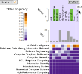
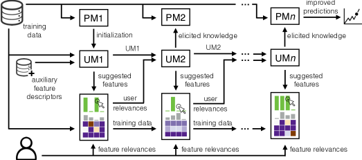
Figure 1: Overview of our approach. (a) The user interface of an implementation of our approach. (b) Flow of data between the prediction model (PM), user model (UM) and interactive visualization at various iterations of the prior knowledge elicitation and prediction improvement process. See the ‘Method’ section for details.

1 Introduction

We address the machine learning problem of predicting values of a target variable given a training data set in which the target variable values are known. The training data set needs to be representative of the underlying population, and its size must be large enough for the machine learning model to accurately learn to predict the target variable. Yet, in applications like personalized medicine [9, 26, 34], brain imaging [36, 38] and textual document categorization [14, 21, 22, 27, 37], the number of features by far exceeds the number of samples, leading to the “small $n$ large $p$” problem [12] where classical models inaccurately predict the target. Fitting regression models for this problem requires regularizing the model’s regression coefficients [16, 35, 39]. Typically, the level of regularization is tuned by estimating a hyperparameter from the data, but this neglects prior information that could be available on the problem, the prior information referring to any knowledge of the problem the user may have before inspecting the data. Yet, knowledge of the features’ effects on the target could significantly improve predictions [31].

The use of prior knowledge in prediction is often not straightforward. For example, the prior information may not be available in any format that can easily be plugged into the prediction model. Nevertheless, a domain expert may possess tacit knowledge, not written down anywhere, of the relationships between the features and the target variable. Take, for example, the task of predicting the number of citations a scientific document receives in a certain domain. An expert can easily indicate that the presence of a term ‘neural’ in the document implies a higher relative citation count in the machine learning domain. However, eliciting such tacit knowledge is difficult when the number of putative features is large, and checking each individual feature is excessively laborious.

We present a novel approach that extracts the tacit knowledge from the domain expert and uses this knowledge as prior information for improved predictions. A prediction model is still responsible for generating the predictions for the target variable. However, a user model selects features whose relevance is indicated by the user, a domain expert, using an interactive visualization. Here, a relevant feature is a feature that is positively correlated with the target value. The user model iteratively elicits this information, to build a model of the user’s tacit knowledge and select other features that would benefit from the user’s input. The user input is then encoded into prior knowledge for the prediction model to improve its accuracy. Our contributions are:

• We present a novel method that interactively models the user’s tacit knowledge of the relevance of features to the predicted target, and uses this elicited information as prior knowledge for a more accurate prediction model.

• Through a user study, we demonstrate that using a user model to select the features that require input from the domain expert significantly improves prior knowledge elicitation when compared to randomly selected features.

2 Related Work

Expert knowledge can be integrated into prediction models by defining prior distributions for model parameters. Typically, in prior elicitation full prior distributions have to be defined by experts [13, 17, 19]. This is time consuming and infeasible for high-dimensional problems, even with interactive tools. A simpler method for Bayesian Networks required experts to only indicate the presence or absence of the most uncertain causal relationships [6]. In information retrieval, interactive intent modeling finds relevant resources based on user’s previous input [30]. Deciding which features to ask user input on is done iteratively, by balancing the exploitation of the currently most promising features and the exploration of uncertain, possibly interesting ones. The balancing is done with linear bandit algorithms [3].

Previously, interactive visualization has been used in classification tasks [2, 20, 24]. However, the underlying classification model itself is not directly modified, or the approaches are limited to cases with more samples than features. In [5], possibly important features were visualized to the user and included interactively to a classifier, and in [28] the user was shown features that best explained predictions of a classifier, allowing her to reject irrelevant features. Semi-supervised clustering was considered in [23], where users indicated which pairs of items should belong to the same cluster. However, simply including or excluding a feature is sensitive to errors and not sufficient in “small $n$ large $p$” problems. The method in [32] tackles this problem with the simplifying assumption that the expert may give noisy input directly on the regression coefficients, and  [25] performed non-interactively a direct elicitation of logistic regression coefficients. In recent works considering a similar problem, a user specified the similarity of features as input [1], or features were chosen based on information gain [10].

Our new approach for interactive visualization has the purpose of knowledge elicitation to improve the accuracy of a prediction model. Out approach differs from the methods above by using a ’user model’ which adaptively learns the domain user’s expert knowledge. It automatically guides the interaction towards features that would likely benefit from the user’s input, based on the current representation of the expert’s knowledge. Furthermore, the user model can exploit not only the training data, but also any additional auxiliary data about the features, important in scaling the method to small data sets.

3 Method

Fig. 1 shows the main components of our approach, namely: the prediction model (PM), the user model (UM), and the interactive visualization (IVis). An implementation of our approach is shown in Fig. 1. IVis displays the training data and some features for which the user (a domain expert) has to indicate their relevance for a particular prediction task. UM then models the user’s knowledge of feature relevances, and PM uses the user input with the training data to improve the predictions. The training data (TD) is a small set of samples with a large number of features and the target. Additional data, referred to as auxiliary feature descriptors (AFD), are required to provide information about the features that is not available in the training data. The flow of events in our approach is as follows:

1. Initialize. PM is initialized by TD. UM is initialized by TD, AFD, and information from the learned PM.

Repeat

1. Select features to show. UM is used to select a set of features to show next to the user.

2. Get user’s input. The user indicates the relevances of the shown features for the given prediction task, based on her prior tacit knowledge.

3. Update models. UM and PM are updated using the relevances of the features provided by the user.

Until ready

1. Return predictions. PM returns improved predictions.

We briefly discuss each component below; details are provided in the Supplementary Material.

3.1 Prediction Model

We introduce the idea on a scalar-valued prediction problem with linear models, but the approach can be generalized.

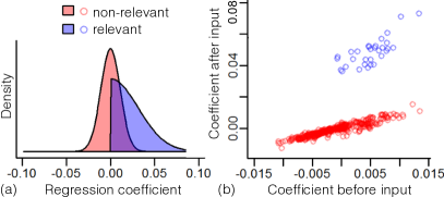
Figure 2: Regression coefficients of relevant and non-relevant features: (a) Prior distributions; (b) Impact of user input.

As input, the prediction model takes the training data points $(\mathbf{x}_{i},y_{i}),~{}i=1,\ldots,N$, where $\mathbf{x}_{i}\in\mathbb{R}^{K}$ are the features and $y_{i}\in\mathbb{R}$ the value of the target variable for sample $i$. In addition, a vector of relevances $\mathbf{r}\in\{0,1\}^{K}$ is provided, where $r_{j}=1$ if the feature is relevant, i.e., has received positive user input, and $r_{j}=0$ otherwise. We assume a linear prediction model

$$y_{i}\sim N(\mathbf{x}_{i}^{T}\mathbf{w},\sigma^{2}),\text{ }i=1,\ldots,N,$$

where $\mathbf{w\in}\mathbb{R}^{K}$ is a vector of regression coefficients and $\sigma^{2}$ the variance of the Gaussian noise. The relevances of the features $\mathbf{r}$ enter the prediction model through modifying the prior distribution of the elements of $\mathbf{w}$ as follows:

$$w_{j} \sim N(0,\sigma_{0}^{2}),\text{ if }r_{j}=0,$$

$$w_{j} \sim\text{half-}N(0,a\sigma_{0}^{2}),\text{ if }r_{j}=1.$$

Half-$N$ denotes the half-normal distribution. The intuition is that if a feature is deemed relevant, its presence is assumed to increase the value of the output variable (Fig. 2a). The multiplier $a$ determines the overall ratio of the effect sizes between relevant and non-relevant features. Fig. 2b shows the impact of this formulation on the estimated regression coefficients.

3.2 User Model

Efficient interaction balances between querying additional input on either the most promising relevant features (exploitation), or on the most uncertain ones (exploration). This is achieved by using the upper confidence bound criterion (UCB) to select features to show to the user, as in the algorithm LINREL [3]. At each iteration $t$, a user is shown $n_{t}$ features with highest UCBs from the previous iteration. The user then specifies a binary relevance $r_{j}\in\{0,1\}$ value to each feature $j$. At each iteration, the user model updates the estimated feature relevances $\hat{r}_{j,t}$ using a linear model:

$$\hat{r}_{j,t}=Z_{j}\hat{\mathbf{v}}_{t}+b\quad\forall\quad j\in 1,\ldots,K$$

where $Z_{j}\in\mathbb{R}^{N_{Z}}$ is a feature descriptor of the $j$th feature and $b$ determines the default relevance. The $\hat{\mathbf{v}}_{t}$ is a vector of regression coefficients, and it is estimated from inputs given so far, using the standard regularized least squares solution. The relevances are converted to interval $(0,1)$ using the logistic transformation.

Feature descriptors $Z_{j}$ are chosen depending on the problem domain, and they can be constructed from the training data and/or any auxiliary data in which the features, but not necessarily the target variable, are available. For example, in the evaluation study, we use the tf-idf [18] of keywords in clusters of scientific documents. The intuition is that keywords that appear in similar documents have similar effect in the prediction task, and should thus have correlated feature descriptors. Finally, the UCBs are defined as $r_{j,t}^{UCB}=\hat{r}_{j,t}+c_{j,t}$, where $c_{j,t}$ is a high probability bound for relevance uncertainty, computed using SupLinUCB in [8].

3.3 Interactive Visualization

A heatmap using a color-blind safe color scale depicts the training data (Fig. 1). Rows indicate categories to which the samples are grouped (e.g., domains in which scientific documents were cited). Columns indicate features selected by the user model for which user input is required (e.g., words in a document). The cell color indicates how strongly, on average, the feature was associated to samples in that category (e.g., the average relative citation count in that domain for documents containing the word), with total bars (in grey) above the heatmap showing the total number of samples on which this value was based, to get an idea of the reliability of the training data. By clicking on the feature labels, the user can set relevance bars (in green) to either 1 or 0, indicating whether that feature is respectively relevant or not to the predicted target (e.g., being cited in the Artificial Intelligence domain). The relevance bars provide the domain expert the means to input her tacit knowledge. Even though the heatmap and the total bars showing the training data could help the domain expert decide the feature relevances, they are not essential for our approach. Nonetheless, we still evaluated their usefulness through a post-questionnaire in our user study (see the ‘Results and Discussion’ section).

4 Evaluation

We conducted computational and empirical experiments to evaluate our approach in a real-world scenario.

The experiment conditions included:

• C1: non-interactive prediction model;

• C2: interactive prediction model with features for user input suggested randomly;

• C3: interactive prediction model with features for user input suggested by the user model.

The task was to predict the relative citation count a scientific document will get in the domain of Artificial Intelligence (target variable) given that it has certain words (features) in the title, abstract or keywords. In C2 and C3, participants had to indicate whether each of the 10 suggested features were relevant or not to the target, for 20 iterations.

The data we used was a subset of Tang et al.’s citation data set [33] containing 162 scientific documents, for which we: (i) manually retrieved the author provided keywords; (ii) automatically extracted additional keywords from the title and abstract of the documents using Python Rake [29] and KP-Miner [11]; (iii) lemmatized all the keywords obtained in i and ii using Python Natural Language Toolkit [4]. This resulted in 457 unique keywords that were used as features. The data collection was evenly split into a training set and a test set. The training set was used to train the prediction model in C1-C3, while the test set was used to evaluate the accuracy of the predictions, using the Mean Squared Error (MSE).

Our hypotheses were:

• H1: C2 and C3 provide more accurate predictions than C1;

• H2: C3 provides more accurate predictions than C2.

We adopted a between-participant design: 12 participants for C2 (8 males); 11 participants for C3 (9 males). All participants: had at least 2 years research experience in machine learning; were undertaking a PhD or postdoc (1st or 2nd year PhD: 4 in C2, 3 in C3); were at least somewhat familiar with heatmaps and bar charts; were aged 20-40. Each participant was trained to use the system (Fig. 1), introduced to the prediction task, and asked to complete the task for one iteration. The answers were then discussed with the experimenter and the participant was given 10 more min to explore the system before the actual experiment. At the end, participants filled in a questionnaire. The experiment took $\approx$30mins and a movie ticket was awarded. For details, see Supplementary Material.

5 Results and Discussion

The final predictions of C2 and C3 were more accurate than those of C1 for all 23 participants, i.e., user input always increased prediction accuracy, and the Mean Squared Error (MSE) decreased as the participants provided more input (Fig. 3a). MSE without user input (C1) was 0.93, and with user input (C2 and C3) after the interaction 0.84 (mean) $\pm$0.05 (sd). Average performance at the end is significantly different from performance without user input (p=2.3e-7, Wilcoxon signed-rank test), confirming H1. Thus, without user input the prediction model explained about 7% of the variance in the target variable, and with user input 16%.

To evaluate the difference between giving user input in a random order (C2) vs. with the user model (C3), we computed the average MSE curves in the two groups (Fig. 3b). The random order improves predictions approximately linearly w.r.t. the number of user input, whereas with the user model the predictions improve more rapidly at early stages of interaction, as expected. We used the maximum distance between the average curves as the test statistic to characterize this difference (Fig. 3b). We computed the distribution of the test statistic, assuming no difference between groups, using $10^{6}$ permutations of the group labels (Fig. 3c), which shows that the difference is significant (p=0.026), thus confirming H2.

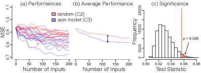
Figure 3: a) Mean squared error w.r.t. the number of inputs provided by our study participants. b) Test statistic is the maximum distance between average performance curves. c) Distribution of the test statistic in $10^{6}$ permutations.

The results of the post-questionnaire (Table 1) indicate that: (i) the visualization of the training data (heatmap+total bars) is used more when the user is uncertain about the feature relevance (as in C2); (ii) when the heatmap is referred to, the total bars are more carefully analysed to verify the reliability of the displayed data (as in C2); and (iii) the visualization is familiar and simple enough for a domain expert to understand and use. In summary, these findings suggest that visualizing the data is useful when eliciting expert feedback, inspiring us to develop the visualization further in the future.

In our approach we query the user about whether a feature is relevant, i.e., is positively correlated with the target variable. This is a compromise between detailed input about regression coefficients (exact value [32] or full prior [13, 17] and simple input discarding a subset of features [6, 28]). This kind of user input is easy to give (difficulty C2 and C3, self-reported in post-study survey: 50% easy, 29% neutral), but powerful in improving the predictive performance. However, the model is potentially sensitive to errors in user input. Also, although providing user input on positive effects was natural for the prediction task considered here, in other cases negative user input may be useful. We will consider these issues further in future work. Our user model formulation has the additional benefit of allowing integration of auxiliary data when defining feature descriptors. This is particularly important when the sample size decreases, and training data alone would not provide enough information to guide user interaction.

	Random (C2)	User model (C3)
Referred to the heatmap	91.7%	75%
Found the heatmap helpful	58.4%	50%
Referred to the total bars	58.3%	25%
Found the total bars helpful	41.7%	16.6%
Found the words relevant	66.7%	75%
Confident with their answers	75%	83.3%
Were not at all confident	8.3%	0%

Table 1: Results of the post-questionnaire (N=23)

6 Conclusion

We have presented a novel approach for eliciting tacit knowledge from domain experts and using it as prior knowledge to improve the accuracy of prediction models for “small $n$ large $p$” problems. A user study indicates the effectiveness of our approach in contrast to a non-interactive prediction model, and one that is interactive but suggests features for user input at random. In the future, we will: evaluate this approach on other real-word data; explore how visualizations can facilitate knowledge elicitation; and investigate ways how to extend the prediction model to multiple output learning.

7 Acknowledgments

We thank the participants of our user study. We acknowledge the computational resources provided by the Aalto Science-IT project. This work was funded by the Academy of Finland (Centre of Excellence in Computational Inference Research COIN, and grants no. 295503, 294238, 286607 and 294015), and by Jenny and Antti Wihuri Foundation.

Supplementary Material

Interactive Elicitation of Knowledge on Feature Relevance Improves Predictions in Small Data Sets

Luana Micallef*^,1, Iiris Sundin*^,1, Pekka Marttinen*^,1, Muhammad Ammad-ud-din¹, Tomi Peltola¹, Marta Soare¹, Giulio Jacucci², and Samuel Kaski¹

¹Helsinki Institute for Information Technology HIIT,
Department of Computer Science, Aalto University, Finland
²Helsinki Institute for Information Technology HIIT,
Department of Computer Science, University of Helsinki, Finland
^∗Authors contributed equally
firstname.lastname@hiit.fi

This supplementary provides addition information about the prediction model (Section 8), the user model (Section 9), and our evaluation (Section 10).

8 Prediction Model

As input, the prediction model takes training data points $(\mathbf{x}_{i},y_{i}),~{}i=1,\ldots,N,$ where $\mathbf{x}_{i}\in\mathbb{R}^{K}$ and $y_{i}\in\mathbb{R}$, and a vector of relevances $\mathbf{r}\in\{0,1\}^{K},$where $r_{j}=1,$ if the feature is relevant, i.e., has received positive feedback. Otherwise, $r_{j}=0$.

We assume the target $y_{i}$ depends linearly on the predictor $\mathbf{x}_{i}$

$$y_{i}\sim N(\mathbf{x}_{i}^{T}\mathbf{w},\sigma^{2}),\text{ }i=1\ldots,N,$$

where $\mathbf{w\in}\mathbb{R}^{K}$ is a vector of regression coefficients and $\sigma^{2}$ is the variance of the Gaussian noise. The relevances of the predictors $\mathbf{r}$ affect the prior distributions of the elements of $\mathbf{w}$ as follows

$$w_{j} \sim N(0,\sigma_{0}^{2}),\text{ if }r_{j}=0,$$

$$w_{j} \sim\text{half-}N(0,a\sigma_{0}^{2}),\text{ if }r_{j}=1.$$

Here, half-$N$ denotes the half-normal distribution. The intuition is that if a feature is relevant, the corresponding regression weight is assumed to have a prior distribution constrained to be positive (see, Fig. 4A). The multiplier $a$ determines the ratio of the variance parameters between relevant and non-relevant features, and is given a prior distribution

$$a\sim 1+\text{half-}N(0,12.5\pi).$$

This constrains $a$ to be greater than $1$ and have mean 6, according to a weakly informative prior (see Fig. 4B). This corresponds to the expectation that regression coefficients of the relevant features are greater in magnitude than the coefficients of the non-relevant features.

The term $\sigma_{0}^{2}$ appearing in the prior variances of the regression coefficients of both relevant and non-relevant features is specified by investigating the variance of the linear predictions. A direct integration of regression weights $\mathbf{w}$, conditional on parameters $a$ and $\sigma_{0}^{2}$, gives

$$E_{\mathbf{w}}\left[Var(\mathbf{x}^{T}\mathbf{w)}\right] =\frac{1}{N}{\textstyle\sum\nolimits_{i}}\mathbf{x}_{i}^{T}E_{\mathbf{w}}\left[\mathbf{ww}^{T}\right]\mathbf{x}_{i}$$

$$=\sigma_{0}^{2}(n_{-}+an_{+})+\frac{2a\sigma_{0}^{2}}{\pi}\sum_{k\in R}\sum_{\begin{subarray}{c}h\in R\\ h\neq k\end{subarray}}\sigma_{kh}$$ (1)

$$\approx\sigma_{0}^{2}(n_{-}+an_{+}),$$ (2)

where $n_{+}$ and $n_{-}$ are the numbers of relevant and non-relevant features, $R$ is the set of all relevant features, and $\sigma_{kh}$ is the covariance between the $k^{th}$ and $h^{th}$ features. In practice the second term in Equation 1 is less than 25% of the first term, and therefore, we retain only the first term to keep the computations simple (this is exact when the relevant features are uncorrelated). Let $\xi$ denote the proportion of variance explained by the prediction model. Assuming $y$ is normalized, the proportion of variance explained is given by Equation 2, and we can solve for $\sigma_{0}^{2}$ for any $\xi$ by using:

$$\sigma_{0}^{2}(n_{-}+an_{+})=\xi,$$

which yields

$$\sigma_{0}^{2}=\frac{\xi}{n_{-}+an_{+}}.$$ (3)

We define a prior for $\xi$ as

$$\xi\sim Beta(1,9),$$

shown in Fig. 4C, which corresponds to the expectation that approximately 10% of the variance of the target is explained by the prediction model. This further imposes a prior on $\sigma_{0}^{2}$ through Equation 3. Finally, we place the following prior on noise variance

$$\sigma\sim\text{half-}N(0,1),$$

which completes the definition of the prediction model. The model is implemented using the probabilistic programming language Stan [7].

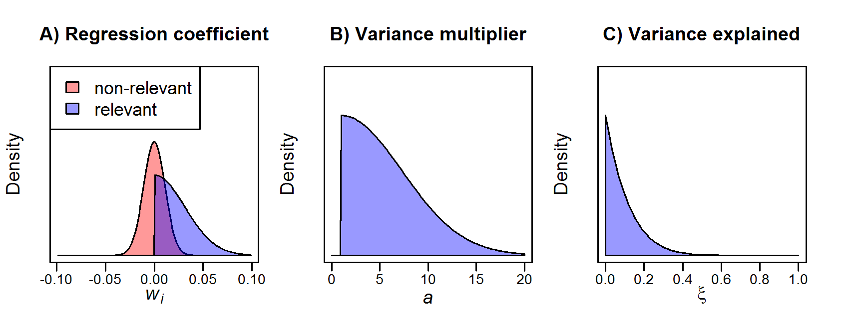
Figure 4: Prior distributions of the parameters of the prediction model

9 User Model

Efficient interaction balances between querying additional input on either the most promising relevant features (exploitation), or on the most uncertain ones (exploration). The upper confidence bound criterion (UCB) to select features to show to the user achieves this, as in the algorithm LINREL [3]. At each iteration $t$, a user is shown $n_{t}$ features with the highest UCBs from the previous iteration. The user then specifies a binary relevance $r_{j}\in\{0,1\}$ value to each feature $j$. We denote the inputs collected from the user before or at iteration $t$ by $\mathbf{r}_{t}\in\mathbb{R}^{\sum_{i=1}^{t}n_{i}}$. At each iteration, the user model updates the estimated feature relevances $\hat{r}_{j,t}$ using a linear model:

$$\hat{r}_{j,t}=Z_{j}\hat{\mathbf{v}}_{t}+b\quad\forall\quad j\in 1,\ldots,K$$

where $Z_{j}\in\mathbb{R}^{N_{Z}}$ is a feature descriptor of the $j$th feature and $b$ determines the default relevance. $\hat{\mathbf{v}}_{t}$ is a vector of regression coefficients, and it is estimated from inputs given so far, using a standard formula for regularized regression:

$$\hat{\mathbf{v}}_{t}=(Z_{t}^{\top}Z_{t}+\lambda\mathbf{I})^{-1}Z_{t}^{\top}(\mathbf{r}_{t}-b),$$

where $\lambda$ is a regularizer, $Z\in\mathbb{R}^{K,N_{Z}}$ a feature descriptor matrix, and its sub-matrix $Z_{t}$ contains the descriptors corresponding to features that have received user input thus far. Furthermore, we convert the relevances to the interval $(0,1)$ using the logistic transformation.

A high probability bound, $c_{j,t}$, for the relevance uncertainty $P\left(|\tilde{r}_{j}-\hat{r}_{j,t}|\leqslant c_{j,t}\right)\leqslant 1-\delta$, where $\tilde{r}_{j}$ is the true relevance, can be derived using SupLinUCB [8]:

$$c_{j,t}=\rho_{t}\sqrt{Z_{j}^{\top}(Z_{t}Z_{t}^{\top}+\lambda\mathbf{I})^{-1}Z_{j}},\hskip 11.38092pt\rho_{t}=\sqrt{\alpha\log\big{(}\frac{2tK}{\delta}\big{)}}.$$

The UCBs are then defined as

$$r_{j,t}^{UCB}=\hat{r}_{j,t}+c_{j,t}.$$

The parameter $\alpha$ determines the exploration-exploitation trade-off. In the Evaluation, $n_{t}=10\quad\forall\quad t\in 1,\ldots,20$, $b$=0.5, $\lambda$=1e-3, $\alpha$=0.5 and $\delta$=0.05. The user model selects the features with the largest UCBs that have not yet been selected, to avoid querying the same feature twice.

Initialization

We initialize the user model with pseudo-input in order to choose as relevant first 10 features as possible. We use the feature’s regression coefficient $w_{j}$ from the non-interactive prediction model as pseudo-input, since the input to the features with the highest regression coefficients has the greatest potential in improving the predictions [32]. The impact of pseudo-input is set to be weak, so that 10 pseudo-inputs correspond to one real user input. Therefore the impact of pseudo-feedback decreases as more user input is received.

Pseudo-input can be included in $\mathbf{r_{t}}$, or, if expressed explicitly as $\mathbf{r_{0}}$, the regression coefficients are

$$\hat{\mathbf{v}}_{t}=(Z_{t}^{\top}Z_{t}+\beta Z^{\top}Z+\lambda\mathbf{I})^{-1}(Z_{t}^{\top}(\mathbf{r}_{t}-b)+\beta Z^{\top}(\mathbf{r_{0}}-b)),$$

where $Z$ contains the feature descriptors of all features, and $\beta$=0.01 defines the strength of the pseudo-input.

Feature Descriptors in Evaluation

For the evaluation study, we use tf-idf [18] of words in clusters of scientific documents as feature descriptors. The intuition is that words that appear in similar documents have similar effect in the prediction task, and should thus have correlated feature descriptors. Furthermore, words that appear evenly in all clusters are likely not very useful for the prediction.

The feature descriptors $Z_{j}$ are constructed using auxiliary data on keywords from [15], in combination with our prediction data set. From the auxiliary data, only the documents that had at least one common keyword with the prediction data set were used. This results in 8554 unique documents with 26333 unique (lemmatized) keywords as features. We can use all data available on the features (in both training and test samples) because target variables are not used when constructing feature descriptors. In so doing we utilize maximal amount of information available without risking over-fitting the model.

The documents were clustered to 20 clusters by hierarchical clustering based on their cosine distance in the feature space. Randomly chosen 1000 documents were used to train the model, and the rest of the documents were assigned to clusters based on distance to cluster centers. This results in a feature descriptor matrix $Z\in\mathbb{R}^{K,20}$, where the element $z_{j,c}$ is the tf-idf of a word $j$ in cluster $c$. The tf-score of a word is computed cluster-wise, and idf document-wise.

10 Evaluation

The following are the documents provided to the participants during the controlled experiment for the training phase and the actual experiment task phase, and the questionnaire participants had to fill in at the end of the experiment together with its results.

See pages - of evaluation_training+task.pdf See pages - of evaluation_postquestionnaire.pdf See pages - of evaluation_postquestionnaire_results.pdf

References

- [1] Afrabandpey, H., Peltola, T., and Kaski, S. Interactive prior elicitation of feature similarities for small sample size prediction. arXiv preprint arXiv:1612.02802 (2016).
- [2] Alsallakh, B., Hanbury, A., Hauser, H., Miksch, S., and Rauber, A. Visual methods for analyzing probabilistic classification data. IEEE Transactions on Visualization and Computer Graphics 20, 12 (2014), 1703–1712.
- [3] Auer, P. Using confidence bounds for exploitation-exploration trade-offs. Journal of Machine Learning Research 3 (2003), 397–422.
- [4] Bird, S. NLTK: the natural language toolkit. In Proc of the COLING/ACL on Interactive presentation sessions (2006), 69–72.
- [5] Brooks, M., Amershi, S., Lee, B., Drucker, S. M., Kapoor, A., and Simard, P. FeatureInsight: Visual support for error-driven feature ideation in text classification. In Proc of IEEE VAST (2015), 105–112.
- [6] Cano, A., Masegosa, A. R., and Moral, S. A Method for integrating expert knowledge when learning Bayesian networks from data. IEEE Transactions on Systems, Man, and Cybernetics, Part B (Cybernetics) 41, 5 (2011), 1382–1394.
- [7] Carpenter, B., Gelman, A., Hoffman, M., Lee, D., Goodrich, B., Betancourt, M., Brubaker, M. A., Guo, J., Li, P., and Riddell, A. Stan: A probabilistic programming language. Journal of Statistical Software (2016 (in press)).
- [8] Chu, W., Li, L., Reyzin, L., and Schapire, R. E. Contextual bandits with linear payoff Functions. In Proc of AISTATS (2011), 208–214.
- [9] Costello, J. C., Heiser, L. M., Georgii, E., Gönen, M., Menden, M. P., Wang, N. J., Bansal, M., Hintsanen, P., Khan, S. A., Mpindi, J.-P., et al. A community effort to assess and improve drug sensitivity prediction algorithms. Nature Biotechnology 32, 12 (2014), 1202–1212.
- [10] Daee, P., Peltola, T., Soare, M., and Kaski, S. Knowledge elicitation via sequential probabilistic inference for high-dimensional prediction. arXiv preprint arXiv:1612.03328 (2016).
- [11] El-Beltagy, S. R., and Rafea, A. KP-Miner: A keyphrase extraction system for English and Arabic documents. Information Systems 34, 1 (2009), 132–144.
- [12] Friedman, J., Hastie, T., and Tibshirani, R. The elements of statistical learning, vol. 1. Springer, Berlin: Springer Series in Statistics, 2001.
- [13] Garthwaite, P. H., Al-Awadhi, S. A., Elfadaly, F. G., and Jenkinson, D. J. Prior distribution elicitation for generalized linear and piecewise-linear models. Journal of Applied Statistics 40, 1 (2013), 59–75.
- [14] Genkin, A., Lewis, D. D., and Madigan, D. Large-scale Bayesian logistic regression for text categorization. Technometrics 49, 3 (2007), 291–304.
- [15] Glowacka, D., Ruotsalo, T., Konuyshkova, K., Athukorala, K., Kaski, S., and Jacucci, G. Directing exploratory search: reinforcement learning from user interactions with keywords. In Proc of IUI, ACM (New York, NY, USA, 2013), 117–128.
- [16] Hoerl, A. E., and Kennard, R. W. Ridge regression: Biased estimation for nonorthogonal problems. Technometrics 12, 1 (1970), 55–67.
- [17] Jones, G., and Johnson, W. O. Prior elicitation: Interactive spreadsheet graphics with sliders can be fun, and informative. The American Statistician 68, 1 (2014), 42–51.
- [18] Jones, K. S. A statistical interpretation of term specificity and its application in retrieval. Journal of Documentation 28 (1972), 11–21.
- [19] Kadane, J. B., Dickey, J. M., Winkler, R. L., Smith, W. S., and Peters, S. C. Interactive elicitation of opinion for a normal linear model. Journal of the American Statistical Association 75, 372 (1980), 845–854.
- [20] Kapoor, A., Lee, B., Tan, D., and Horvitz, E. Interactive optimization for steering machine classification. In Proc of the SIGCHI Conference on Human Factors in Computing Systems, ACM (2010), 1343–1352.
- [21] Kogan, S., Levin, D., Routledge, B. R., Sagi, J. S., and Smith, N. A. Predicting risk from financial reports with regression. In Proc of NAACL HLT (2009), 272–280.
- [22] Lewis, D. D. Feature selection and feature extraction for text categorization. In Proc of the Workshop on Speech and Natural Language (1992), 212–217.
- [23] Lu, Z., and Leen, T. K. Semi-supervised clustering with pairwise constraints: A discriminative approach. In Proc of AISTATS (2007), 299–306.
- [24] May, T., Bannach, A., Davey, J., Ruppert, T., and Kohlhammer, J. Guiding feature subset selection with an interactive visualization. In Proc of IEEE VAST (2011), 111–120.
- [25] O’Leary, R. A., Choy, S. L., Murray, J. V., Kynn, M., Denham, R., Martin, T. G., and Mengersen, K. Comparison of three expert elicitation methods for logistic regression on predicting the presence of the threatened brush-tailed rock-wallaby. Environmetrics 20 (2009), 379–398.
- [26] Papillon-Cavanagh, S., De Jay, N., Hachem, N., Olsen, C., Bontempi, G., Aerts, H. J., Quackenbush, J., and Haibe-Kains, B. Comparison and validation of genomic predictors for anticancer drug sensitivity. Journal of the American Medical Informatics Association 20, 4 (2013), 597–602.
- [27] Qu, L., Ifrim, G., and Weikum, G. The bag-of-opinions method for review rating prediction from sparse text patterns. In Proc of COLING/ACL (2010), 913–921.
- [28] Ribeiro, M. T., Singh, S., and Guestrin, C. "Why should I trust you?": Explaining the predictions of any classifier. In Proc of ACM SIGKDD (2016).
- [29] Rose, S., Engel, D., Cramer, N., and Cowley, W. Automatic keyword extraction from individual documents. Text Mining (2010), 1–20.
- [30] Ruotsalo, T., Jacucci, G., Myllymäki, P., and Kaski, S. Interactive intent modeling: Information discovery beyond search. CACM 58, 1 (2015), 86–92.
- [31] Sinha, A. P., and Zhao, H. Incorporating domain knowledge into data mining classifiers: An application in indirect lending. Decision Support Systems 46, 1 (2008), 287–299.
- [32] Soare, M., Ammad-ud-din, M., and Kaski, S. Regression with by expert knowledge elicitation. In Proc of ICMLA (to appear). arXiv preprint arXiv:1605.06477 (2016).
- [33] Tang, J., Zhang, J., Yao, L., Li, J., Zhang, L., and Su, Z. Arnetminer: extraction and mining of academic social networks. In Proc of ACM SIGKDD (2008), 990–998.
- [34] Tian, L., Alizadeh, A. A., Gentles, A. J., and Tibshirani, R. A simple method for estimating interactions between a treatment and a large number of covariates. Journal of the American Statistical Association 109, 508 (2014), 1517–1532.
- [35] Tibshirani, R. Regression shrinkage and selection via the lasso. Journal of the Royal Statistical Society. Series B (Methodological) (1996), 267–288.
- [36] Wang, H., Nie, F., Huang, H., Risacher, S., Ding, C., Saykin, A. J., Shen, L., et al. Sparse multi-task regression and feature selection to identify brain imaging predictors for memory performance. In Proc of ICCV (2011), 557–562.
- [37] Zhang, T., Popescul, A., and Dom, B. Linear prediction models with graph regularization for web-page categorization. In Proc of ACM SIGKDD (2006), 821–826.
- [38] Zhou, H., Li, L., and Zhu, H. Tensor regression with applications in neuroimaging data analysis. Journal of the American Statistical Association 108, 502 (2013), 540–552.
- [39] Zou, H., and Hastie, T. Regularization and variable selection via the elastic net. Journal of the Royal Statistical Society: Series B (Statistical Methodology) 67, 2 (2005), 301–320.