Comparative Evaluation of Big-Data Systems on Scientific Image Analytics Workloads

Abstract

Scientific discoveries are increasingly driven by analyzing large volumes of image data. Many new libraries and specialized database management systems (DBMSs) have emerged to support such tasks. It is unclear, however, how well these systems support real-world image analysis use cases, and how performant are the image analytics tasks implemented on top of such systems. In this paper, we present the first comprehensive evaluation of large-scale image analysis systems using two real-world scientific image data processing use cases. We evaluate five representative systems (SciDB, Myria, Spark, Dask, and TensorFlow) and find that each of them has shortcomings that complicate implementation or hurt performance. Such shortcomings lead to new research opportunities in making large-scale image analysis both efficient and easy to use.

1 Introduction

With advances in data collection and storage technologies, data analysis has become widely accepted as the fourth paradigm of science [12]. In many scientific fields, an increasing portion of this data is images [17, 18]. It is thus crucial for big data systems to provide a scalable and efficient means to store and analyze such data, and support programming models that can be easily utilized by domain scientists (e.g., astronomers, physicists, biologists, etc).

As an example, the Large Synoptic Survey Telescope (LSST) is a large-scale international initiative to build a new telescope for surveying the visible sky [22] with plans to collect 60 petabytes of images over 10 years. In previous astronomy surveys (e.g., the Sloan Digital Sky Survey (SDSS)),the collected images were processed by an expert team of engineers on dedicated servers, with results distilled into textual catalogs for other astronomers to analyze. In contrast, one of the goals of LSST is to broaden access to the collected images to astronomers around the globe, and enable them to run analyses on the images themselves. Similarly, in neuroscience, several large collections of imaging data are being compiled. For example, the UK biobank will release Magnetic Resonance Imaging (MRI) data from close to 500k human brains (more than 200 TB) for neuroscientists to analyze [24]. Multiple other initiatives are similarly making large collections of image data available to researchers [2, 20, 37].

Such use cases emphasize the need for effective tools to support the management and analysis of image data: tools that are efficient, scale well, and are easy to program without requiring deep systems expertise to deploy and tune.

Surprisingly, there has been only limited work from the data management research community in building tools to support large-scale image management and analytics. Rasdaman [30] and SciDB [32] are two well-known DBMSs that specialize in the storage and processing of multidimensional array data and they are a natural choice for implementing image analytics. Most other work developed for storing image data targets predominantly image storage and retrieval based on keyword or similarity searches [9, 5, 6]. Recently developed parallel data processing libraries such as Spark [35] and TensorFlow [1] can also support image data analysis. Hence, the key questions that we ask in this paper are: How well do these existing big data systems support the management and analysis requirements of real scientific workloads? Is it easy to implement large-scale analytics using these systems? How efficient are the resulting applications that are built on top of such systems? Do they require deep technical expertise to optimize?

In this paper, we present the first comprehensive study of the issues mentioned above. Specifically, we choose five big data systems that encompass all major paradigms of parallel data processing: a domain-specific DBMS for multidimensional array data (SciDB [32]), a general-purpose cluster computing library with persistence capabilities (Spark [35]), a traditional parallel general-purpose DBMS (Myria [15, 41]), and a general-purpose (Dask [31]) and domain-specific (TensorFlow [1]) parallel-programming library. To evaluate these systems, we take two typical end-to-end image analytics pipelines from astronomy and neuroscience. Each pipeline comes with a reference implementation in Python provided by the domain scientists. We then attempt to re-implement them using the five big data systems and deploy the resulting implementation on commodity hardware available in the public cloud to simulate the typical hardware and software setup in domain scientists’ labs. We then evaluate the resulting implementations with the following goals in mind:

• Investigate if the given system can be used to implement the pipelines, and if so how easy is it to do so (Section 4).

• Measure the performance of the resulting pipelines built on top of such systems, in terms of execution time when deployed on a cluster of machines (Section 5.1 and Section 5.2).

• Evaluate the system’s ability to scale, both with the number of machines available in the cluster, and the size of the input data to process (Section 5.1).

• Assess the tunings, if any, that each system requires to correctly and efficiently execute each pipeline (Section 5.3).

Our study shows that, in spite of coming from different domains, the two real-world use cases have important similarities. Input data takes the form of multidimensional arrays encoded using domain-specific file formats (FITS, NIfTI, etc.). Data processing involves slicing along different dimensions, aggregations, stencil (a.k.a. multidimensional window) operations, spatial joins as well as other complex transformations expressed in Python. We find that all big data systems have important limitations. SciDB and TensorFlow, having limited or no support for user-provided Python code, require rewriting entire use cases in their own languages. Such rewrite is difficult and sometime impossible due to missing operations. Meanwhile, optimized implementations of specific operations can significantly boost performance when available. No system works directly with scientific image file formats, and all systems require manual tuning for efficient execution. We could implement both use cases in their entirety only on Myria and Spark. We implemented the entire neuroscience use case on Dask also, but found the tool too difficult to debug for the astronomy use case. Interestingly, Spark and Myria, which offer data management capabilities, do so without extra overhead compared with Dask, which has no such capability. Overall, while performance and scalability results are promising, we find much room for improvement in efficiently supporting image analytics at scale.

2 Evaluated Systems

In this section we briefly describe the five evaluated systems and their design choices pertinent to image analytics. The source code of all systems are publicly available.

SciDB [4] is a shared-nothing DBMS for storing and processing multidimensional arrays. To use SciDB, users first ingest data into the system, which are stored as arrays divided into chunks distributed across nodes in a cluster. Users then query the stored data using the Array Query Language (AQL) or Array Functional Language (AFL) through the provided Python interface. SciDB supports user-defined functions in C++ and, recently, Python (with the latter executed in a separate Python process). In SciDB, query plans are represented as an operator tree, where operators, including user-defined ones, process data iteratively one chunk at a time.

Spark [42] is a cluster-computing system. Spark works on data stored in HDFS or Amazon S3. Spark’s data model is centered around the Resilient Distributed Datasets (RDD) abstraction [42], where RDDs can both reside in memory or on disk distributed across nodes in a cluster. RDDs are akin to relations partitioned across the cluster and as such Spark’s data model is similar to that of relational systems. Spark offers a SQL interface, but users can also manipulate RDDs using Scala, Java, or Python APIs, with the latter executed in a separate Python process as Spark is implemented using Scala. Programs that manipulate RDDs are represented as graphs. When executed, the Spark scheduler determines which node in the graph can be executed and starts by serializing the required objects and data to one of the machines.

Myria [15, 41] is a shared-nothing DBMS developed at the University of Washington. Unlike SciDB and Spark, Myria can both directly process data stored in HDFS/S3 or ingest data into its own internal representation. Myria uses the relational data model and PostgreSQL [29] as its node-local storage subsystem. Users write queries in MyriaL, an imperative-declarative hybrid language, with SQL-like declarative query constructs and imperative statements such as loops. Besides MyriaL, Myria supports Python user-defined functions and aggregates that can be included in queries. Myria query plans are represented as a graph of operators. When executed, each operator pipelines data without materializing it to disk. To support Python user-defined functions, Myria supports the blob data type, which allows users to write queries that directly manipulate NumPy arrays or other specialized data types by storing them as blobs.

Dask [8] is a general-purpose parallel computing library for Python. Dask does not provide data persistence. Like Spark, Dask distributes data and computation across nodes in a cluster for arbitrary Python programs. Unlike Spark, users do not express their computation using specialized data abstractions. Instead, users describe their computation using standard Python constructs, except that computation to be distributed in the cluster is explicitly marked as delayed using Dask’s API. When Dask encounters such labeled code, it constructs a compute graph of operators, where operators are either Python language constructs or function calls. When the results of such delayed computation is needed (e.g., they are written to files), Dask’s scheduler determines which machine to execute the delayed computation, and serializes the required function and data to that machine before starting its execution. Unless explicitly instructed, the computed results remain on the machine where the computation took place.

TensorFlow [1] is a library for numerical computation from Google. Like Dask, TensorFlow does not provide data persistence. It provides C++ and Python APIs for users to express operations over N-dimensional tensors. Such operations are organized into dataflow graphs, where nodes represent computation, and edges are the flow of data expressed using tensors (which can be serialized to and from other data structures such as NumPy arrays). TensorFlow optimizes these computation graphs and can execute them locally, in a cluster, on GPUs, and even on mobile devices. Similar to the above systems, the master distributes the computation when deployed on a cluster. The schedule, however, is specified by the programmer. Additionally, all data ingest goes through the master and results are always returned to the master.

3 Image Analytics Use Cases

We use two real-world scientific image analytics use cases from neuroscience and astronomy as evaluation benchmarks.

3.1 Neuroscience

Many sub-fields of neuroscience use image data to make inferences about the brain [21]. Data sizes have dramatically grown recently due to an increase in data collection efforts [2, 20]. The use case we focus on analyzes Magnetic Resonance Imaging (MRI) data in human brains. Specifically, we focus on diffusion MRI (dMRI), where the directional profile of diffusion can be used to infer the directions of brain connections. This method has been used to estimate large-scale brain connectivity, and relate the properties of brain connections to brain health and cognitive functions [40].

3.1.1 Data

The input data comes from the Human Connectome Project [39]. We use data from the S900 release, which includes dMRI data from over 900 healthy adult subjects collected between 2012 and 2015.

The dataset contains dMRI measurements obtained at a nominal spatial resolution of 1.25$\times$1.25$\times$1.25 $mm^{3}$. Measurements were repeated 288 times in each subject, with different gradient directions and diffusion weightings. Each measurement’s data, called a volume or image volume, is stored in a 3D (145$\times$145$\times$174) array of floating point numbers, with one value per three-dimensional pixel (a.k.a. a voxel).

Information about gradient directions and diffusion weightings is captured in the image metadata and is reflected in the imageID for each image volume. Each subject’s 288 measurements include 18 in which no diffusion weighting was applied. These volumes are used for calibration of the diffusion-weighted measurements.

Each subject’s data is stored in standard NIfTI-1 [26] image format and contains the 4D data array (i.e., 288 3D image volumes), totaling 1.4GB in compressed form, which expands to 4.2GB when uncompressed. We use up to 25 subjects’ data (or a little over 100GB) for this use case.

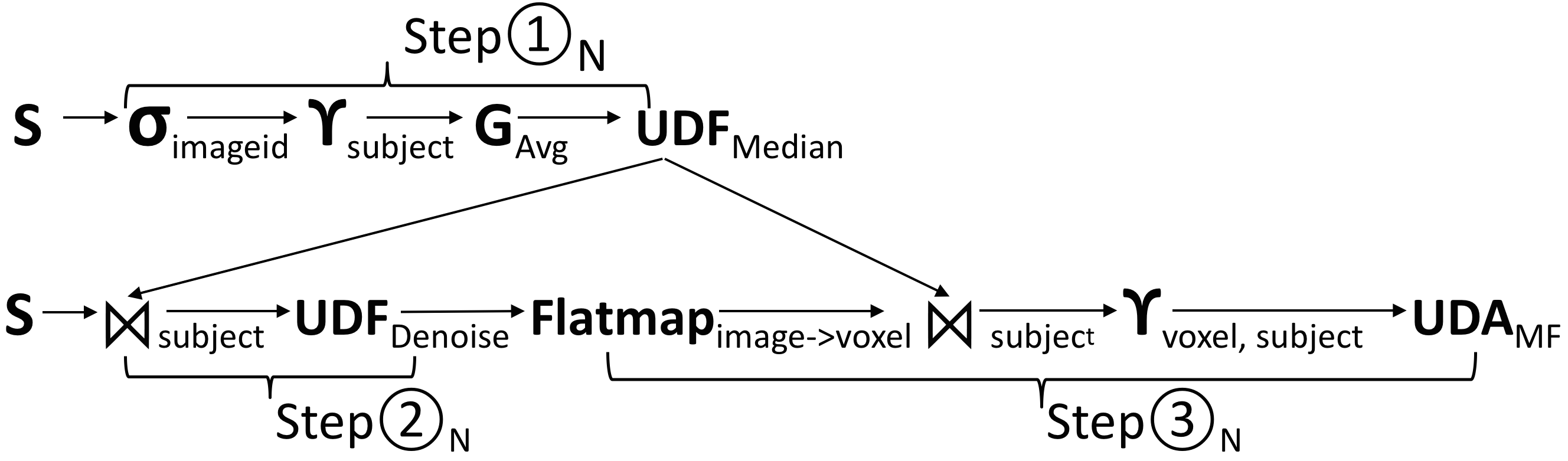
Figure 1: Neuroscience use case: Step _N Segmentation, Step _N Denoising, and Step _N Model fitting.

3.1.2 Processing Pipeline

Shown in Figure 1, the benchmark contains three steps from a typical dMRI image analysis pipeline for each subject. Step  _N performs volume segmentation to identify and extract the subset of each image volume that contains the brain (as opposed to the skull and the background) Step  _N denoises the extracted image volumes. Finally, Step  _N fits a physical model of diffusion to each voxel across all volumes of each subject. We describe each step in detail next.

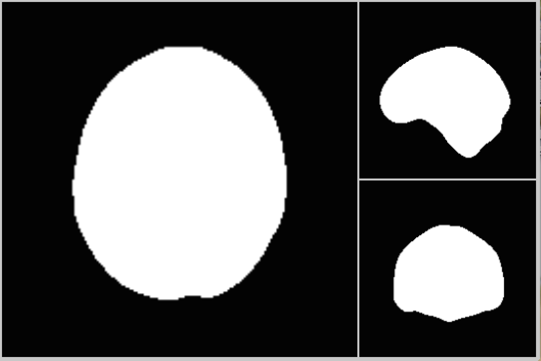
(a) Mask values.

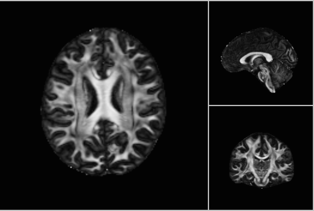
(b) FA values.

Figure 2: Orthogonal slices of Mask and Fractional Anisotropy values for a single subject.

Segmentation: Step  _N constructs a 3D mask that segments each image volume into two parts: one with the part to be analyzed, i.e., the brain, and the other with uninteresting background. As the brain comprises around two-thirds of the image volume, using the generated mask to filter out the background will speed up subsequent steps. Segmentation proceeds in three sub-steps. First, we select the subset of volumes with no diffusion weighting applied. These images are used for segmentation as they have higher signal-to-noise ratio. Next, we compute a mean image from the selected volumes by averaging the value of each voxel. Finally, we apply the Otsu segmentation algorithm [27] to the mean volume to create a mask volume per subject. As an illustration, 2(a) shows the orthogonal slices of the binary mask for a single subject.

Denoising: Denoising is needed to improve image quality and accuracy of the analysis results. In our pipeline, the denoising step (Step  _N) can be performed on each volume independently. Denoising operates on a 3D sliding window of voxels using the non-local means algorithm [7], where we use the mask from Step  _N to denoise only parts of the image volume containing the brain.

Model fitting: Finally, Step  _N computes a physical model of diffusion. We use the diffusion tensor model (DTM) for this purpose, which summarizes the directional diffusion profile within a voxel as a 3D Gaussian distribution [3]. Fitting the DTM is done per voxel and can be parallelized across voxels. Logically, this step is a flatmap operation that takes a volume as input and outputs multiple voxel blocks. All 288 values for each voxel block are then grouped together before fitting the DTM for each voxel. Given the 288 values in a voxel, fitting the model requires estimating a 3$\times$3 variance/covariance matrix (a rank 2 tensor).

The model parameters are summarized as a scalar for each voxel called Fractional Anistropy (FA) that quantifies diffusivity differences across different direction. 2(b) shows orthogonal slices of the FA values for a single subject.

Our reference implementation is written in Python and Cython using Dipy [13] and executes as a single process on one machine.

3.2 Astronomy

As discussed in Section 1, astronomy surveys are generating an increasing amount of image data. Our second use case is an abridged version of the LSST image processing pipeline [23], which includes analysis routines that astronomers would typically perform on such data.

3.2.1 Data

We use data from the High cadence Transient Survey [16] for this use case, as data from the LSST survey is not yet available. This telescope scans the sky through repeated visits to individual, possibly overlapping, locations. We use up to 24 visits that cover the same area of the sky in the evaluation. Each visit is divided into 60 sensor images, with each consisting of an 80MB 2D image (4000$\times$4072 pixels) with associated metadata. The total amount of data from all 24 visits is approximately 115GB.

Figure 4 shows the co-added exposures from 24 visits for one location on the sky. The images are encoded using FITS format [10] with a header and data block. The data block has three 2D arrays, with each element containing flux, variance, and mask for every pixel.

Figure 3: Astronomy use case: Step  _A Pre-Processing, Step  _A Patch Creation, Step  _A Co-addition, and Step  _A Source Detection.

Figure 4: Coadded image of 24 visits to the same place on the sky. Spaces between exposures show sensor boundaries.

3.2.2 Processing Pipeline

Our benchmark contains four steps from the LSST processing pipeline as shown in Figure 3:

Pre-Processing: We pre-process each input exposure with background estimation and subtraction, detection and repair of cosmetic defects and cosmic rays, and aperture corrections for the photometric calibration. This can be executed in parallel on each image. The output is called a calibrated exposure.

Patch Creation: The analysis partitions the sky into rectangular regions called patches. Step  _A maps each calibrated exposure to the patches that it overlaps. Each exposure can be part of 1 to 6 patches, leading to a logical flatmap operation, which replicates each exposure once for each overlapping patch. As pixels from multiple exposures can contribute to a single patch, this step then groups the exposures associated with each patch and creates a new exposure object for each patch in each visit. The output of this step is an exposure for each patch.

Co-addition: To provide the highest signal-to-noise ratio (SNR) for the exposures for subsequent processing, Step  _A groups the exposures associated with the same patch across different visits and stacks them by summing up the pixel (or flux) values. This is called co-addition and the resulting objects are known as Coadds. Before summing up the pixel values, this step performs iterative outlier removal by computing the mean flux value for each pixel and setting any pixel that is three standard deviations away from the mean to null. Our reference implementation performs two such cleaning iterations.

Source Detection: Finally, Step  _A detects sources visible in each Coadd generated from Step  _A by estimating the background and detecting all pixel clusters with flux values above a given threshold.

Our reference implementation is written in Python, with several internal functions implemented in C++, utilizing the LSST stack [22]. While the LSST stack can run on multiple nodes, the reference is a single node implementation.

4 Qualitative Evaluation

We evaluate the five big data systems along two dimensions. The first dimension, which we present in this section, is the system’s ease of use, which we measure using lines of code (LoC) needed to implement the use cases and a qualitative assessment of overall implementation complexity. We discuss performance and required physical tunings in Section 5.

⬇

1from scidbpy import connect

2sdb = connect(’...’)

3data_sdb = sdb.from_array(data)

4data_filtered = data_sdb.compress(sdb.from_array(gtab.b0s_mask), axis=3) # Filter

5mean_b0_sdb = data_filtered.mean(index=3)# Mean

Figure 5: SciDB implementation of Step  _N in the neuroscience use case. The code uses the Python interface and AFL to ingest data, filter it using the compress function, and compute the mean along the fourth dimension.

4.1 SciDB

Implementation: SciDB is designed for array analytics to be implemented in AQL or AFL, optionally on top of SciDB’s Python API as we illustrate in Figure 5. SciDB, however, lacks critical functions including high-dimensional convolutions (e.g., Step  _N, Step  _N, Step  _A), which makes the reimplementation of the use cases highly nontrivial. We nevertheless were able to rewrite and evaluate two specific operations in SciDB, namely, Step  _N and Step  _A. SciDB recently released an interface called stream(), which allows SciDB to pass its array data to an external process after converting such data to Tab-Separated Values (TSV). We use this interface to implement Step  _N.

We implemented two strategies to ingest ingest neuroscience use case’s NIfTI files into SciDB: SciDB-py’s built-in API (i.e., from_array), and SciDB’s accelerated IO library (i.e., aio_input). For the former, we first convert NIfTI files to NumPy arrays using the NiBabel package [25] and import them into SciDB using from_array(). For the latter, we first convert the NIfTI files into Comma-Separated Value (CSV) files that we then load into SciDB using the aio_input function. We use the latter technique for the FITS files from the astronomy use case.

The SciDB implementation of the neuroscience use case took 155 LoC. Table 1 shows the detailed breakdown by operations. Co-addtion (Step  _A) is expressed in 180 LoC of AQL, along with 85 LoC Python code for ingesting FITS files into SciDB.

	Dask	SciDB	Spark	Myria	TensorFlow
Neuroscience
Re-used Reference	30	3	32	35	0
Data Ingest	33	60	8	5	15
Segmentation	25	40	34	10	121
Denoising	19	52	1	3	128
Model Fit.	11	NA	39	15	NA
Astronomy
Re-used Reference	X	NA	212	225	NA
Data Ingest	X	85	12	5	NA
Pre-proc.	X	X	1	4	NA
Patch Creation	X	X	4	9	NA
Co-Addition	X	180	2	5	NA
Source Detection	X	NA	7	2	NA

Table 1: Lines of code for each implementation. NA not applicable, X not possible to implement.

Qualitative Assessment: It was challenging to rewrite the use cases entirely in AQL/AFL. The recent stream() interface makes it possible to execute legacy Python code, but assumes that TSV can be easily digested by the external process, which required us to convert between TSV and FITS. An alternate approach would have been to replace FITS handlers with TSV handlers in the LSST stack, which might have been more efficient but would definitely be more difficult.

4.2 Spark

Implementation: We use Spark’s Python API to implement both use cases. Our implementation transforms the data into Spark’s pair RDDs, which are parallel collections of key-value pair records. In each RDD, the key attribute is an identifier for an image fragment and the value is the Numpy array with the image data. Our implementation then uses the predefined Spark operations (map, flatmap, groupby) to split and regroup image data following the plan from Figure 1. To avoid joins, we make the mask a broadcast variable, which gets automatically replicated on all workers. We use the Python functions from the reference implementation to perform the actual computations on the values. These functions are passed as arguments, a.k.a., lambdas, to Spark’s map, flatmap, and groupby operations. To ingest data in the neuroscience usecase, we first convert the NIfTI files into NumPy arrays that we stage on Amazon S3.FITS files staged in s3 as they are. During pipeline execution, we read the Amazon S3 data directly into worker memory. Figure 6 shows an abridged version of the code for the neuroscience use case. We implement the astronomy use case similarly.

⬇

1modelsRDD = imgRDD

2 .map(lambda x:denoise(x,mask))

3 .flatMap(lambda x: repart(x, mask))

4 .groupBy(lambda x: (x[0][0],x[0][1]))

5 .map(regroup)

6 .map(fitmodel)

Figure 6: Spark code showing Denoising and Model fitting in the neuroscience use case. Code for the Python functions is not shown.

Qualitative Assessment: Spark’s ability to execute user-provided Python code over its RDD collections and its support for arbitrary python objects as keys made the implementation for both use cases straightforward. We could reuse the reference Python code, with fewer than 85 additional LoC for the neuroscience use case, and fewer than 30 additional LoC for the astronomy one. To ensure efficient execution, however, the Spark implementations of both use cases required tuning the degree of parallelism and locations for data caching as we will describe in Section 5.3.

4.3 Myria

Implementation: Myria’s use case implementation is similar to Spark’s: We specify the overall pipeline in MyriaL, but call Python UDFs and UDAs for all core image processing operations. In the Myria implementation of the neuroscience use case, we execute a query to compute the mask, which we broadcast across the cluster. A second query then computes the rest of the pipeline starting from a broadcast join between the data and the mask. Also similar to Spark, we read the NumPy version of the input data directly from S3. In the neuroscience use case, we ingest the input data into an Image relation, with each tuple consisting of subject ID, image ID and image volume. The image volume, containing a serialized NumPy array, is stored using the Myria blob data type. Figure 7 shows the code snippet for denoising the image volumes in the neuroscience use case. Line 1 to Line 2 connect to Myria and register the denoise UDF. Line 3 then executes the query to join the Images relation with the Mask relation and denoise each image volume.

⬇

1conn = MyriaConnection(url="...")

2conn.create_function("Denoise", Denoise)

3query = MyriaQuery.submit("""

4 T1 = SCAN(Images);

5 T2 = SCAN(Mask);

6 Joined = [SELECT T1.subjId, T1.imgId, T1.img, T2.mask

7 FROM T1, T2

8 WHERE T1.subjId = T2.subjId];

9 Denoised = [FROM Joined EMIT

10 PYUDF(Denoise, T1.img, T1.mask) as

11 img, T1.subjId, T1.imgId]; """ )

Figure 7: Myria code showing Python UDF registration and execution in the denoising step of the neuroscience use case.

We implement the astronomy use case similarly using MyriaL to specify the overall pipeline and code from the reference implementation as UDFs/UDAs for image processing.

Qualitative Assessment: Similar to Spark, our Myria implementation leverages much of the reference Python code, making it easy to implement both use cases. Table 1 shows that only 2 to 15 extra LoC in MyriaL were necessary to implement each operation. Myria required a small amount of tuning for performance and memory management as we describe in Section 5.3.

4.4 Dask

Implementation: As described in Section 2, users specify their computation to Dask by building compute graphs similar to Spark. There are two major differences, however. First, we do not need to reimplement the computation using the RDD abstraction and can construct graphs directly on top of Python data structures. On the other hand, we need to explicitly inform Dask when the constructed compute graphs should be executed, e.g., when the values generated from the graphs are needed for subsequent computation.

As an illustration of constructing compute graphs, Figure 8 shows a code fragment from Step  _N of the neuroscience use case. We first construct a compute graph that downloads and filters each subject’s data on Line 2. Note the use of delayed to construct a compute graph by postponing computation, and specifying that downloadAndFilter is to be called on each subject separately. At this point, only the compute graph is built; data has not been downloaded or filtered.

Next, on Line 5 we request Dask to evaluate the compute graph via the call to result to compute the number of volumes in each subject’s dataset. Calling result introduces a barrier, where the Dask scheduler determines how to distribute the computation to the threads spawn on the worker machines, executes the graph, and blocks until result returns after the numVols has been evaluated. Since we constructed the graph such that downloadAndFilter is called on individual subjects, Dask will parallelize the computation across the worker machines and adjust each machine’s load dynamically.

We then build a new compute graph to compute the average image of the volumes by calling mean. We would like this computation to be parallelized across blocks of voxels, as indicated by the iterator construct on Line 9. Next, the individual averaged volumes are reassembled on Line 10, and calling median_otsu on Line 11 computes the mask.

⬇

1 for id in subjectIds:

2 data[id].vols = delayed(downloadAndFilter)(id)

3

4 for id in subjectIds: # barrier

5 data[id].numVols = len(data[id].vols.result())

6

7 for id in subjectIds:

8 means = [delayed(mean)(block) for block in

9 partitionVoxels(data[id].vols)]

10 means = delayed(reassemble)(means)

11 mask = delayed(median_otsu)(means)

Figure 8: Dask code showing compute graph construction and execution in the segmentation step of the neuroscience use case.

The rest of the neuroscience use case follows the same programming paradigm. We implemented the astronomy use case with the same approach. Interestingly, the implementation freezes once deployed on a cluster and we found it surprisingly difficult to track down the cause of the problem. Hence, we do not report performance numbers for the second use case.

Qualitative Assessment: Dask’s compute graph construction API was relatively easy to use, and we reused most of the reference implementation. We implemented the neuroscience use case in approximately 120 LoC. In implementing the compute graphs, however, we had to reason about when to insert barriers to evaluate the constructed graphs. In addition, we needed to manually specify how data should be partitioned across different machines for each of the stages to facilitate parallelism (e.g., by image volume or blocks of voxels, as specified on Line 9 in Figure 8). Choosing different parallelism strategies impacts the correctness and performance of the implementation. Beyond that, the Dask scheduler did well in distributing tasks across machines based on estimating data transfer and computation costs.

4.5 TensorFlow

Implementation: As TensorFlow’s API operates on tensors, we need to fully rewrite the reference use case implementation using the API. Given the complexity of the use cases, we only implement the neuroscience one. Additionally, we implement a somewhat simplified version of the final mask generation operation in Step  _N. We further rewrite Step  _N using convolutions, but without filtering with the mask as TensorFlow does not support element-wise data assignment.

In TensorFlow, the master node handles data distribution: it converts the input data to tensors, and distributes it to the worker nodes. In our implementation, the master reads the data directly from Amazon S3.

TensorFlow’s support for distributed computation is currently limited. The developer must manually map computation and data to each worker as TensorFlow does not provide automatic static or dynamic work assignment. Although the entire use case could be implemented in one graph, size limitation necessitates multiple graphs as each compute graph must be smaller than 2GB when serialized. Given this limitation, we implement the use case in steps: we build a new compute graph for each step (as shown in Figure 1) of the use case. We distribute the data for each step to the workers and execute the step. We add a global barrier to wait for all workers to return their results before proceeding, with the master node converts between NumPy arrays and tensors as needed. Figure 9 shows the code for the main part of the mean computation in Step  _N. The first loop assigns the input data with shape sh (Line 8) and the associated code (Line 9) to each worker. Then, we process the data in batches of size equal to the number of available workers on Line 19.

⬇

1# steps contains the predefined mapping

2# from data to workernodes

3pl_inputs = []

4work = []

5# The first for loop defines the graph

6for i_worker in range(len(steps[0])):

7 with tf.device(steps[0][i_worker]):

8 pl_inputs.append(tf.placeholder(shape=sh))

9 work.append(tf.reduce_mean(pl_inputs[-1]))

10mean_data = []

11# Iterate over the predefined steps

12for i in range(len(steps)):

13 this_zs = zs[i*len(steps[0]):

14 i*len(steps[0]) + len(steps[i])]

15 # Define the input to be fed into the graph

16 zip_d = zip(pl_inputs[:len(steps[i])],

17 [part_arrs[z] for z in this_zs])

18 # Executes the actual computation - incl. barrier

19 mean_data += run(work[:len(steps[i])], zip_d)

Figure 9: TensorFlow code fragment showing compute graph construction and execution.

Qualitative Assessment: Like SciDB, TensorFlow requires a complete rewrite of the use case, which takes a significant amount of time. Similar to Dask, TensorFlow requires that users manually specify data distribution across machines. The 2GB limit on graph size further complicates the implementation as we describe above. Finally, the implementation requires tuning the degree of parallelism as we will describe in Section 5.3.

5 Quantitative Evaluation

In this section, we evaluate the performance of the implemented use cases and the system tunings necessary for successful and efficient execution. All experiments are performed on the Amazon Web Services cloud using the r3.2xlarge instance type, with each instance having 8 vCPU, 61GB of Memory, and 160GB SSD storage.

5.1 End-to-End Performance

Subjects	1	2	4	8	12	25
Input	4.1	8.4	16.8	33.6	50.4	105
Largest Intermediate	8.4	16.8	33.6	67.2	100.8	210

(a) Neuroscience data sizes (GB)

Visits	2	4	8	12	24
Input	9.6	19.2	38.4	57.6	115.2
Largest Intermediate	24	48	96	144	288

(b) Astronomy data sizes (GB)

(c) Neuroscience: End-to-end runtime with varying data size

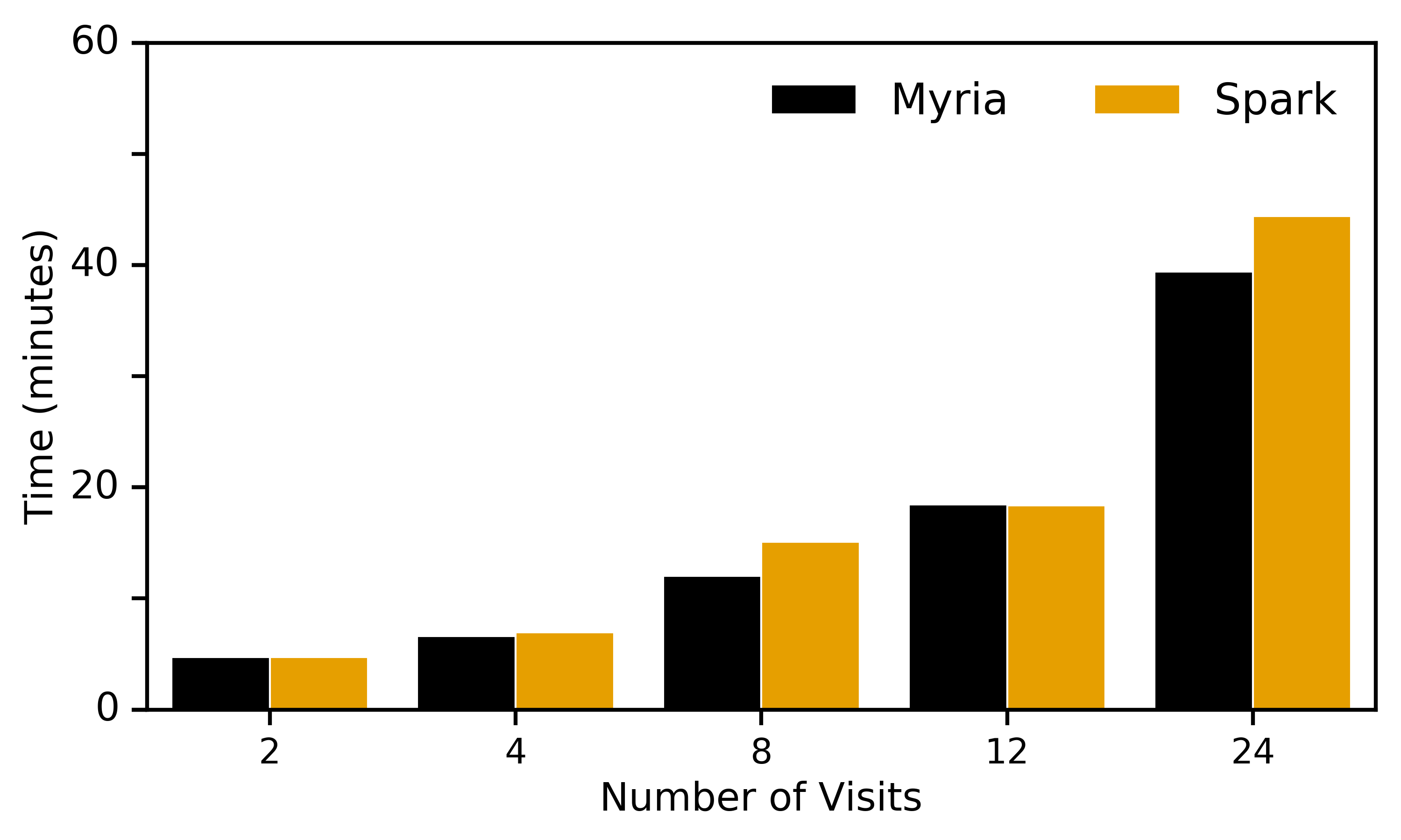
(d) Astronomy: End-to-end runtime with varying data size

Subjects	1	2	4	8	12	25
Dask	1	0.60	0.45	0.36	0.33	0.32
Myria	1	0.77	0.64	0.60	0.61	0.58
Spark	1	0.72	0.61	0.60	0.58	0.59

(e) Neuroscience: Normalized runtime per subject

Visits	2	4	8	12	24
Spark	1	0.73	0.79	0.64	0.78
Myria	1	0.69	0.63	0.65	0.69

(f) Astronomy: Normalized runtime per visit

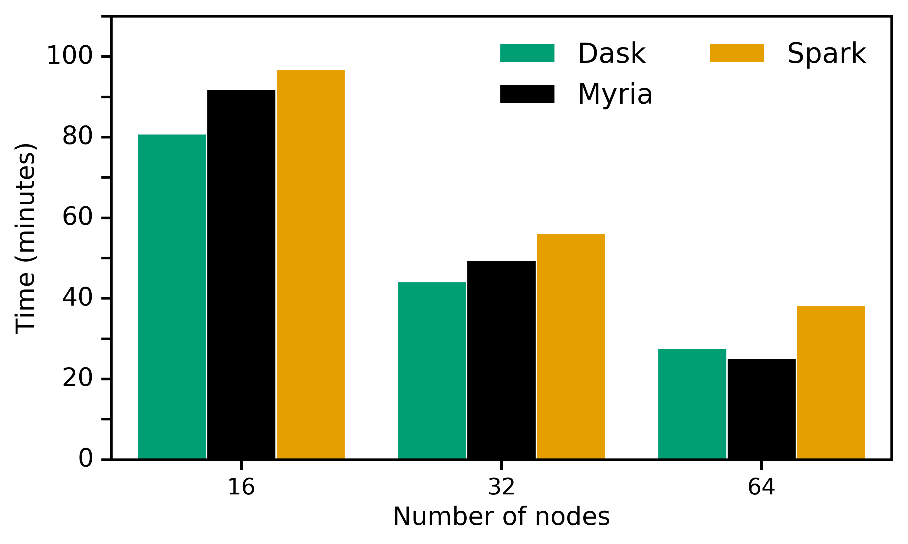
(g) Neuroscience: End-to-end runtime with varying cluster size

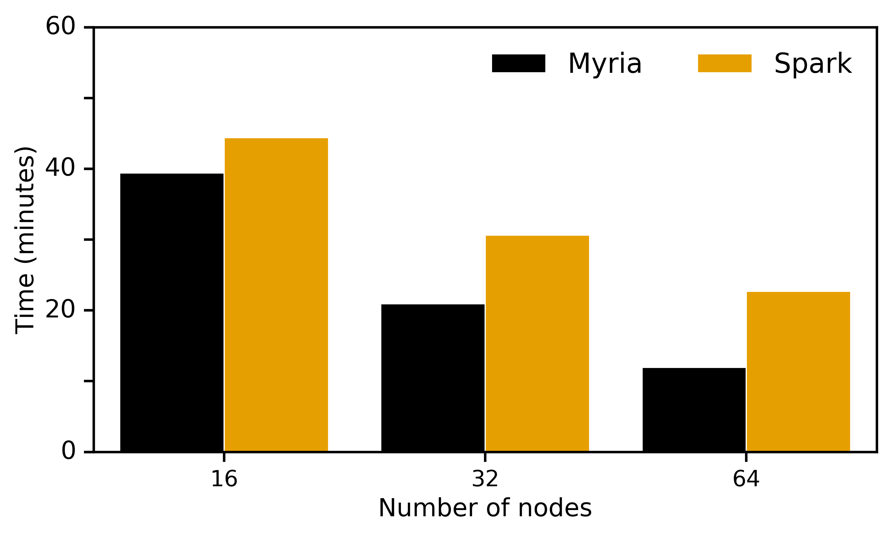
(h) Astronomy: End-to-end runtime with varying cluster size

Figure 10: Overall performance: results for end-to-end experiments for Neuroscience and Astronomy use cases.

We evaluate the performance of running the two use cases end-to-end. We focus on Dask, Myria, and Spark, the three systems that we were able to execute one or both benchmarks entirely. We start the execution with data stored in Amazon S3 and execute all use case steps. We materialize the final output in worker memories. We seek to answer three questions: How does the performance compare across the three systems? How well do the systems scale as we grow the input data or the cluster? What is the penalty, if any, for executing the use case on top of data processing systems such as Myria or Spark compared with Dask, a library designed for the distributed execution of Python code? To answer these questions, we first fix the cluster size at 16 nodes and vary the input data size. For the neuroscience use case we vary the number of subjects from 1 to 25. The data for each subject is approximately 4.25GB in size. The input data thus grows up to a little over 100GB as shown in 10(a). For the astronomy use case, we vary the number of visits from 2 to 24. The data for each visit is approximately 4.8GB in size, for a total of a little over 100GB as shown in 10(b). Because intermediate query results are larger than the input data, we also show the size of the largest intermediate relation for each use case. In the second experiment, we use the largest input data size for each use case and vary the cluster size from 16 to 64 nodes to measure system speedup.

10(c) and 10(d) show the results as we vary the input data size. All three systems achieve comparable performance, which is expected as they execute the same Python code on similarly partitioned data. Interestingly, these results indicate that there is no significant overhead in using the Myria and Spark data processing systems compared with simply using Dask. Dask is at best 14% faster than the other two systems. The faster performance is due in part to Dask’s more efficient pipelining in the context of this specific use case. In Dask, each subject’s data is located on the same node and processing for the next step can start as soon as the subject’s data has been processed by the preceding step. There are no dependencies between subjects. Spark and Myria partition data for every subject across multiple nodes and must thus wait for the preceding step to output the entire RDD or relation respectively, and shuffle tuples as needed before proceeding to the next step. Interestingly, design differences related to data caching and pipelining during execution (see Section 2) do not impact performance in a visible way between Myria and Spark. Dask’s performance exhibits a trend somewhat different from the other two systems. As 10(c) shows, Dask is slower by 60% for single subject but faster for larger numbers compared with Spark and Myria. 10(e) and 10(f) show the runtimes per subject, i.e., the ratios of each pipeline runtime to that obtained for one subject. As the data size increases, these ratios drop, indicating that the systems become more efficient as they amortize start-up costs. Dask’s efficiency increase is most pronounced, indicating that the tool has the largest start-up overhead.

10(g) and 10(h) show the pipeline runtimes for all systems as we increase the cluster size and process the largest, 100GB datasets. All systems show near linear speedup for both use cases. Myria achieves almost perfect linear speedup. Dask is better than Myria on smaller cluster sizes but scheduling overhead makes Dask less efficient as cluster sizes increase, as the scheduler attempts to move tasks among different machines via aggressive work stealing.

Note that we tuned each of the systems to achieve the timings reported above. We discuss the impact of these tunings in Section 5.3.

5.2 Individual Step Performance

Next we focus on the performance of a subset of the pipeline operations that we successfully implemented in TensorFlow and SciDB in addition to the other three systems above.

5.2.1 Data Ingest

The input data for the use cases was staged in Amazon S3. While Myria and Spark can read data directly from S3, repeated operations on the same data can benefit from data being cached either in cluster memory (for Spark) or in local storage across the cluster (for Myria). Other systems must ingest data before processing it. In this section, we measure the time it takes to ingest data.

For Myria, we measure the time to read data from S3 and store it internally in the per-node PostgreSQL instances. For Spark, we measure the time to load data into in-memory RDDs. For both systems, we first preprocess the NifTi files into individual image volumes, which we persist as pickled NumPy files per image in S3 before the ingest, the conversion time is included in the data ingest time. For Dask and TensorFlow, we measure the time to load the data from NifTi files into in-memory NumPy arrays. Finally, for SciDB, we measure the time to ingest the data from NIfTI files into an internal multidimensional array spread across the SciDB cluster. Figure 11 shows the results.

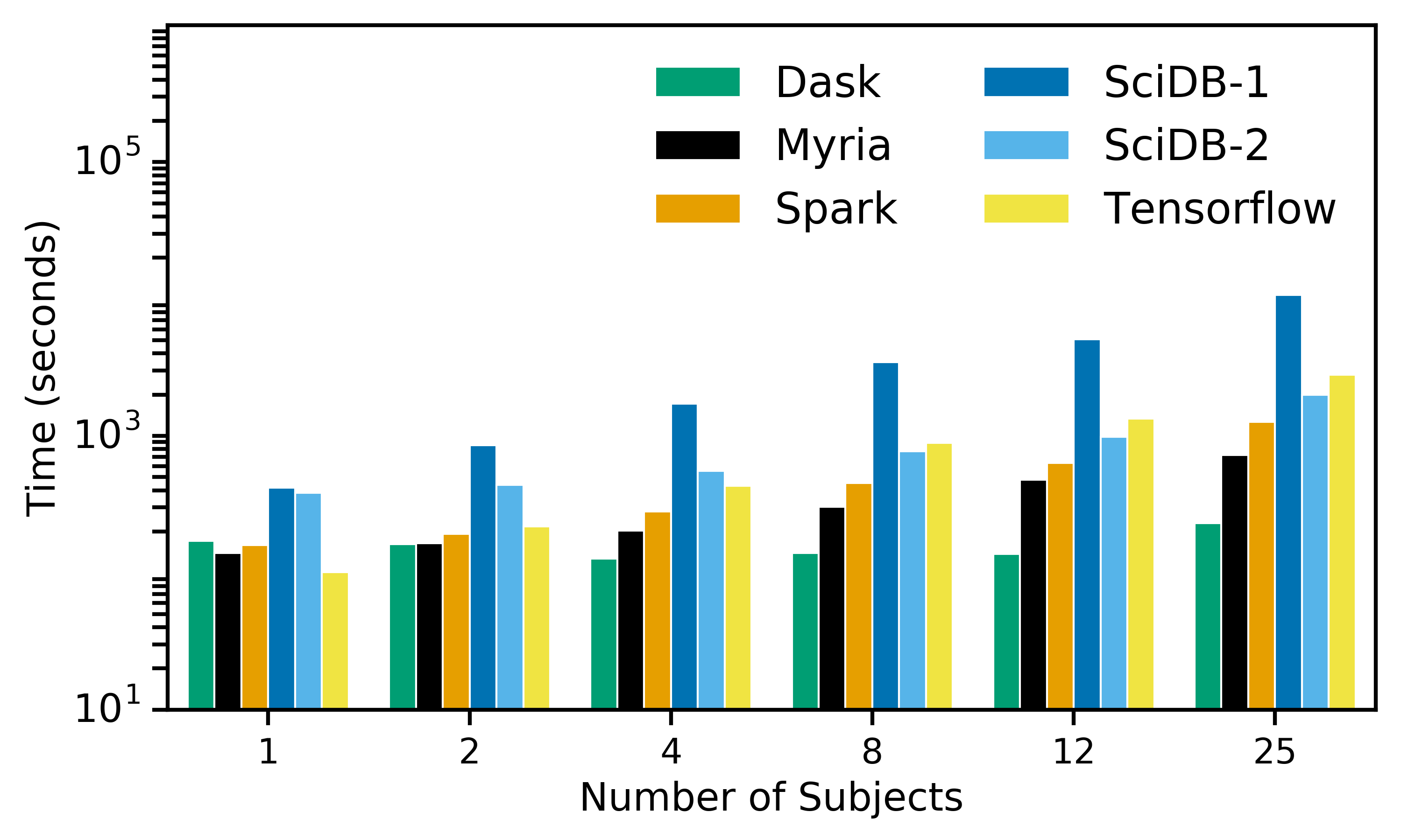
Figure 11: Data ingest times for the neuroscience benchmark on a 16-node cluster. Y-axis uses a log scale.

As the figure shows, data ingest times vary greatly across systems (note the log scale on the y axis). Spark and Myria both download data in parallel on each of the workers from S3. Spark’s API requires the name of the S3 bucket and enumerates the data files on the master node before scheduling the parallel download on the workers, while Myria can directly work with a csv list of files avoiding overhead and is faster than Spark for this step even though it writes the data locally to disk.

For Dask, we explicitly specify the number of subjects to download per node, since each machine only has enough memory to fit the data for up to 3 subjects, and Dask’s scheduler would schedule random number of subjects per machine as it does not know how much data will be downloaded. As a result, Dask’s data ingest time remains constant until the number of subjects exceeds 16, and we assign a subset of machines to download data for more than one subject. The TensorFlow implementation downloads all data to the master node and sends partitions to each node in a pipelined fashion, which is slower than the parallel ingest available in other tools.

We report two sets of timings for SciDB in Figure 11. SciDB-1 reports the time to ingest NumPy arrays with from_array() interface, and SciDB-2 reports the time to convert NIfTI to CSV and ingest using the aio_input library. The aio_input() function is an order of magnitude faster than the pythonAPI based ingest for SciDB and is on par with parallel ingest on Spark and Myria. However, the NIfTI-to-CSV conversion overhead for SciDB is a little larger than the NIfTI-to-NumPy overhead for Spark and Myria, which makes SciDB ingest slower than Spark and Myria.

5.2.2 Neuroscience Use Case: Segmentation

Segmentation is the first step in the neuroscience use case (i.e., Step  _N). We measure the performance of two operations in this step: filtering the data to select a subset of the image volumes, and computing an average image volume for each subject. 12(a) and 12(b) show the runtimes for these two operations as we vary the input data size on the 16-node cluster.

Myria and Dask are the fastest systems on the data filtering step. Myria pushes the selection down to PostgreSQL, which efficiently scans the data and returns only the matching records. Dask is also fast on this operation as all its data is already in memory and the operation is a simple filter. Spark is an-order of magnitude slower than Dask, even though data is in memory for both systems. This is due to Spark’s need to serialize Python code and data among machines. In TensorFlow, the data (tensors) takes the form of 4D arrays. For each subject, the 4D array represents the 288 3D data volumes. We need to filter on the volume ID, which is the fourth dimension. TensorFlow, however, only supports filtering along the first dimension. We thus need to flatten the 4D array apply the selection, and reshape the array back into a 4D structure. As reshaping is expensive compared with filtering, TensorFlow is orders of magnitude slower than the other engines on this operation.

SciDB is slower than some other systems mainly because the internal chunks are not aligned with the selection. That is, in addition to simply reading data chunks, SciDB does more work including extracting subsets out of the chunks and reconstructing them into the resultant arrays.

12(b) shows the result for the mean image volume computations. SciDB is the fastest for mean computation on the small datasets as it is optimized for array operations and this computation exercises SciDB’s specialized design. Spark and Myria demonstrate super-linear scalability for this operation and are comparable with SciDB at larger scales. This is because, at smaller scales, the number of workers used during the mean operation is approximately equal to the number of groups, and there is one group per subject, resulting in low cluster utilization. Dask, meanwhile, performs slower than the other three engines for small datasets due to startup overheads and the overhead of aggressive work stealing. TensorFlow incurs extra cost in converting from image volume to tensors and is an order of magnitude slower than the other engines.

5.2.3 Neuroscience Use Case: Denoising

12(c) shows the runtime for the denoising Step  _N. For this step, the bulk of the processing happens in the user-defined denoising function. Dask, Myria, Spark, and SciDB all run the same code from the reference implementation on similarly partitioned data, which leads to similar overall performance. As in the case of the end-to-end pipeline, Dask’s higher start-up overhead combined with more efficient subsequent processing leads to slightly worse performance for smaller data sizes but similar performance as the data grows. TensorFlow, once again, incurs the overhead of data conversion between image volumes and tensors. Additionally, in the TensorFlow implementation, we could not use the mask to reduce the computation for each data volume as TensorFlow’s operations can only be applied to whole tensors and cannot be masked. SciDB’s stream() interface, although allows us to automatically process SciDB’s array chunks in parallel, performs slightly worse than Myria, Spark, and Dask. This is due to the fact that stream() connects SciDB and external processes only through data in CSV format, and doing so incurs significant overhead.

5.2.4 Astronomy Use Case: Co-addition

Finally, 12(d) shows the runtimes for the coaddition Step  _A. This step is interesting because it involves iterative processing. Once again, Spark and Myria leverage the reference implementation as user-defined code. The reference implementation performs iterative processing internally, yielding high performance. For SciDB, we reimplemented this step entirely in AQL. Furthermore, we use the official SciDB release, which does not include any optimizations for iterative processing, resulting in runtimes more than one order of magnitude slower than those of the other two engines. We observe, however, that our prior work [34] proposed effective optimizations for iterative processing in array engines. By extending SciDB with incremental iterative processing, we showed a 6$\times$ improvement in the execution of that same step. With this optimization, SciDB’s performance would be on par with Spark and Myria for the larger data sizes. Additionally, we could also implement this step using the new stream interface in SciDB, which should then yield similar performance to Myria and Spark as it would execute the Python reference code. Overall, this experiment shows the importance of efficient iterative processing for real-world image analytics pipelines.

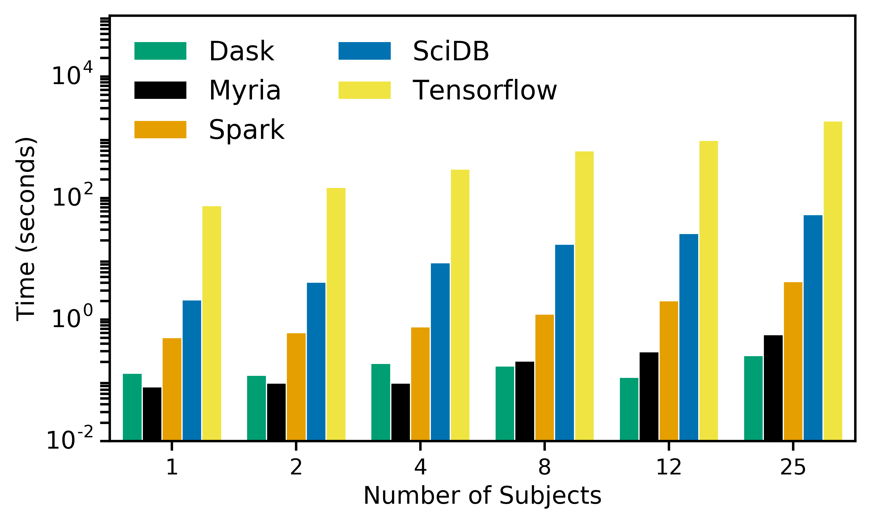
(a) Filter (Segmentation–Neuroscience use case)

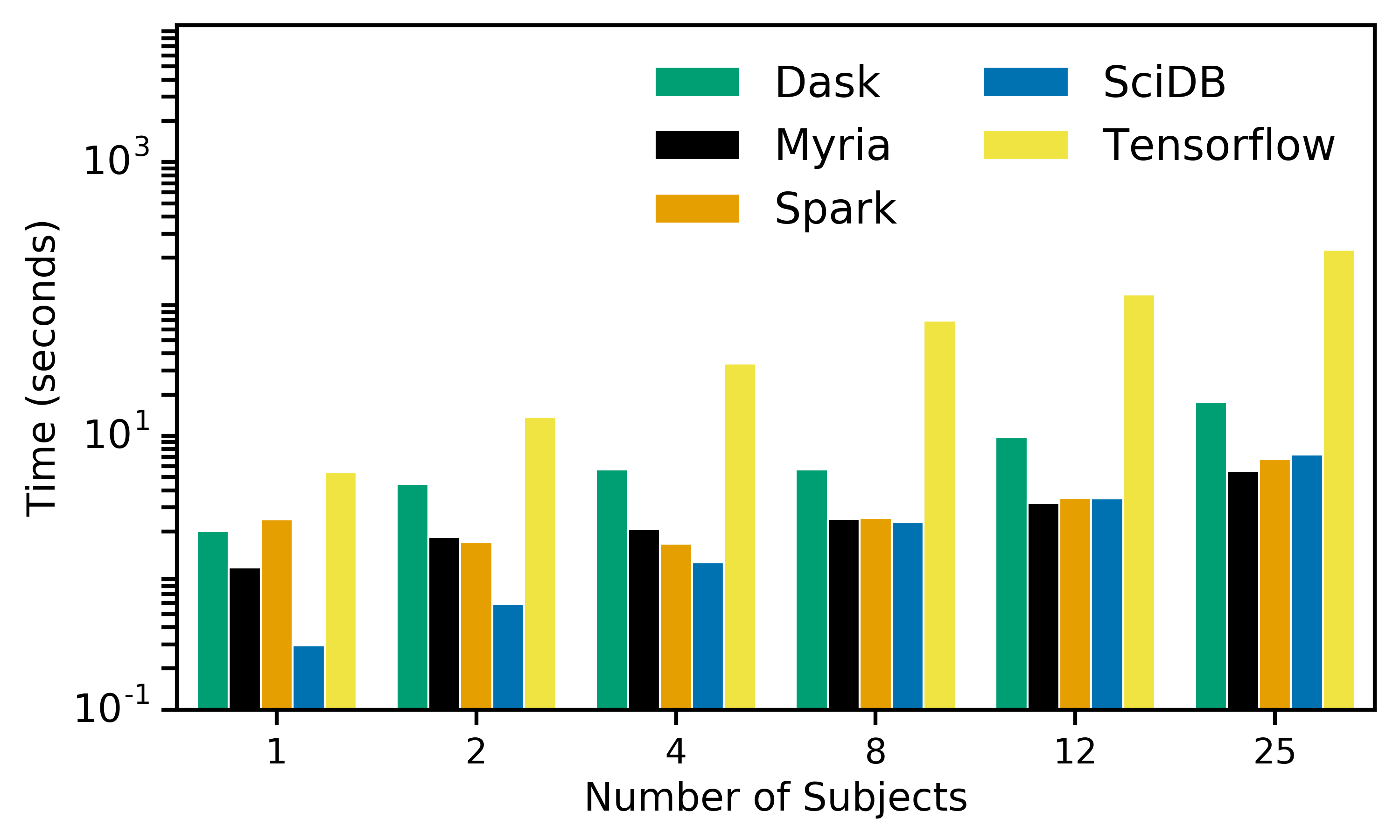
(b) Mean (Segmentation–Neuroscience use case)

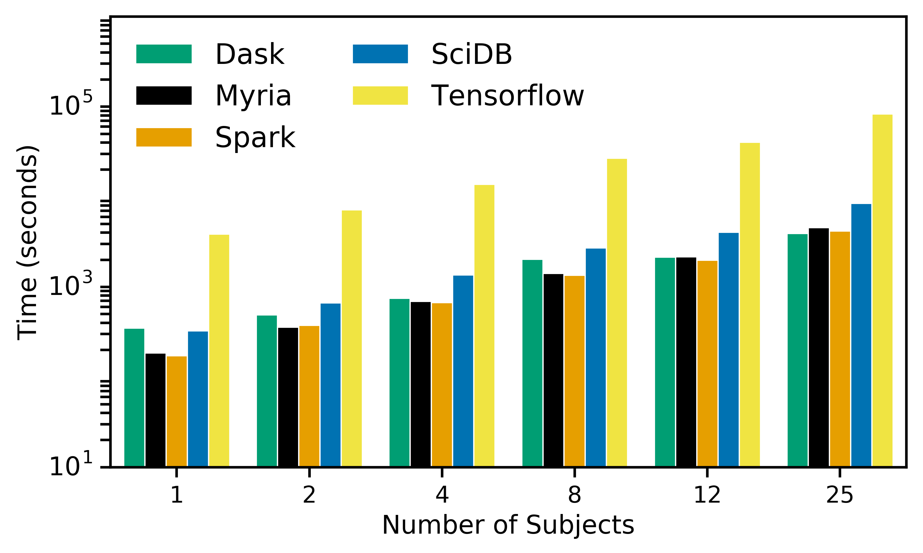
(c) Denoise–Neuroscience use case

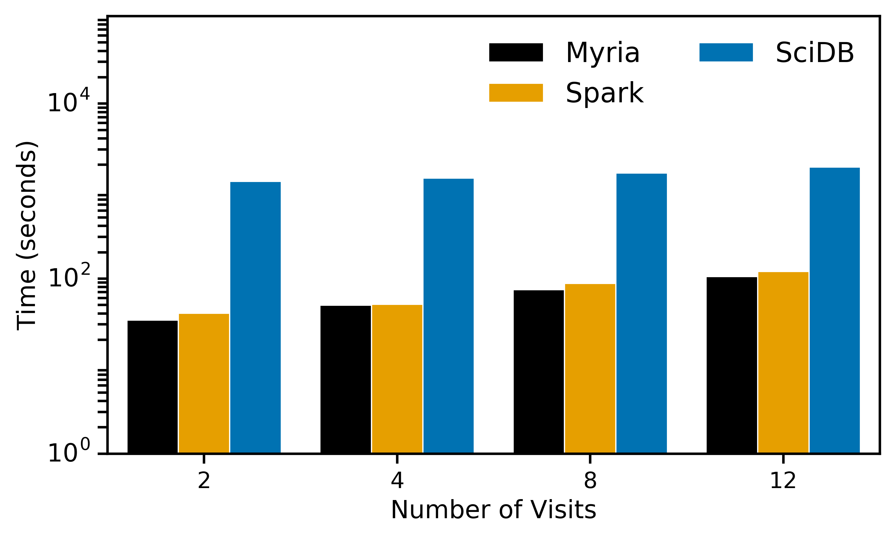
(d) Coaddition–Astronomy use case

Figure 12: Individual step performance (log scale on the y-axis). Experiments run on 16 nodes with largest dataset.

5.3 System Tuning

Finally, we evaluate the five systems on the complexity of the tunings required to achieve high performance.

5.3.1 Degree of Parallelism

Degree of parallelism is a key parameter for big data systems that depends on three factors: (1) the number of nodes in the physical cluster; (2) the number of workers that can execute in parallel on each node; and (3) the size of the data partitions that can be allocated across workers. We evaluated the impact of changing the cluster size in Section 5.1. In this section, we evaluate the impact of (2) and (3).

For Myria, given a 16-node cluster, the degree of parallelism is entirely determined by the number of workers per node. As in traditional parallel DBMSs, Myria hash-partitions data across all workers by default. Figure 13 shows runtimes for different numbers of workers for the neuroscience use case. A larger number of workers yields a higher degree of parallelism but workers also compete for physical resources (memory, CPU, and disk IO). Our manual tuning found that four workers per node yields the best results. The same holds for the astronomy use case (not shown due to space constraints).

Figure 13: Execution time for 25 subjects in the neuroscience use case on Myria for different number of workers per node on a 16 node cluster.

Spark, unlike Myria, creates data partitions (which correspond to tasks), each worker can execute as many tasks in parallel as available cores. Thus, number of workers per node does not impact degree of parallelism when number of cores remains the same. The number of data partitions determines the number of schedulable tasks. Figure 14 shows the query runtimes for different numbers of input data partitions. On a 16-node cluster, the decrease in runtime is dramatic between 1 and 16 partitions, as an increasingly large fraction of the cluster becomes utilized. The runtime continues to improve until 128 data partitions which is the total number of slots in the cluster (i.e., 16 nodes $\times$ 8 cores). Increasing the number of partitions from 16 to 97 results in 50% improvement. Further increases do not improve performance. Interestingly, if the number of data partitions is unspecified, Spark creates a partition for each HDFS block, which typically leads to a small number of large partitions for the data that we use. For example, for the neuroscience use case with a single subject, Spark creates only 4 partitions that results in a highly underutilized cluster. Overall, Spark and Myria both require tuning to achieve best performance. Tuning is simpler in Spark, however, because any sufficiently large number of partitions yields good performance.

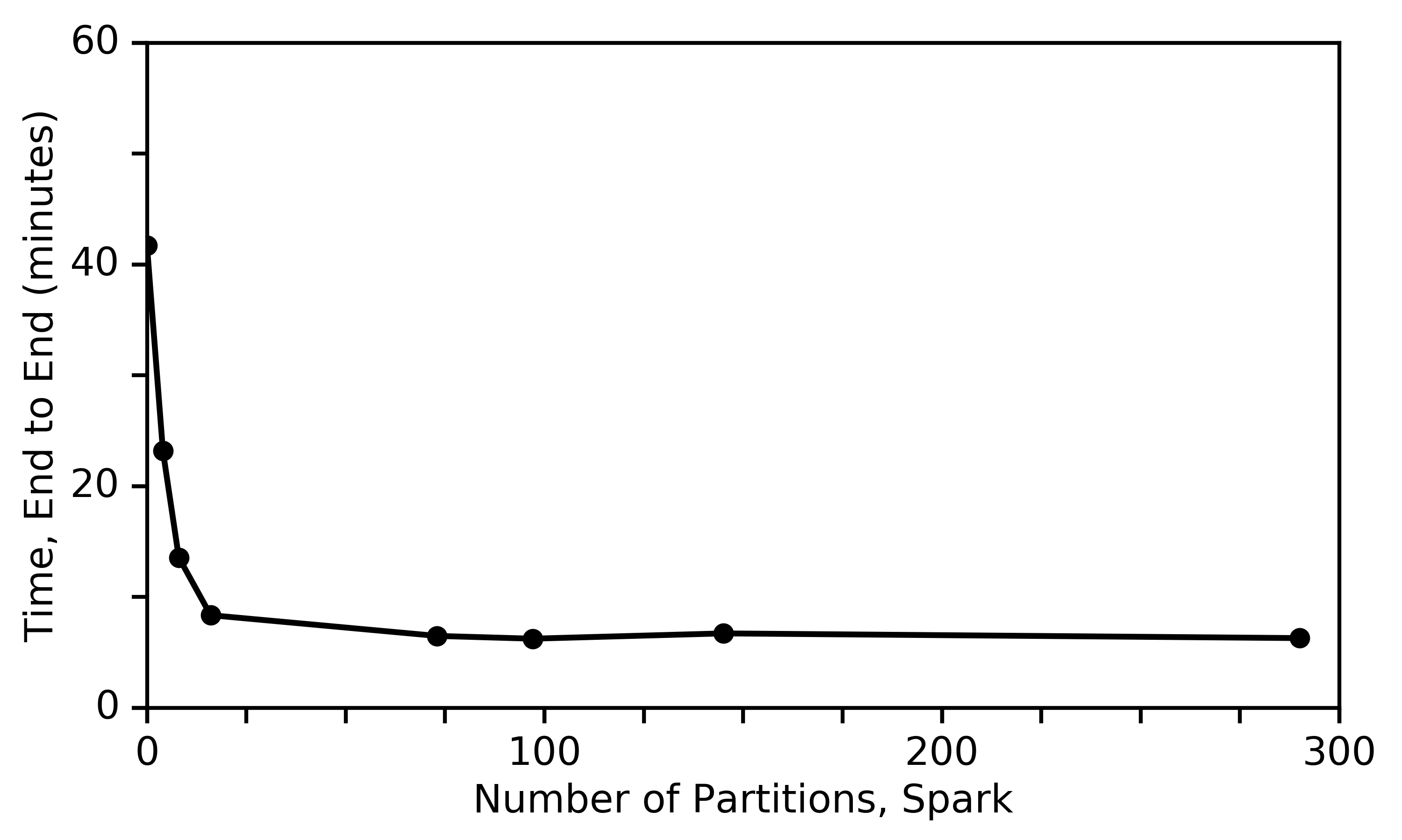
Figure 14: Execution time for a single subject in the neuroscience use case on Spark with varying number of input data partitions.

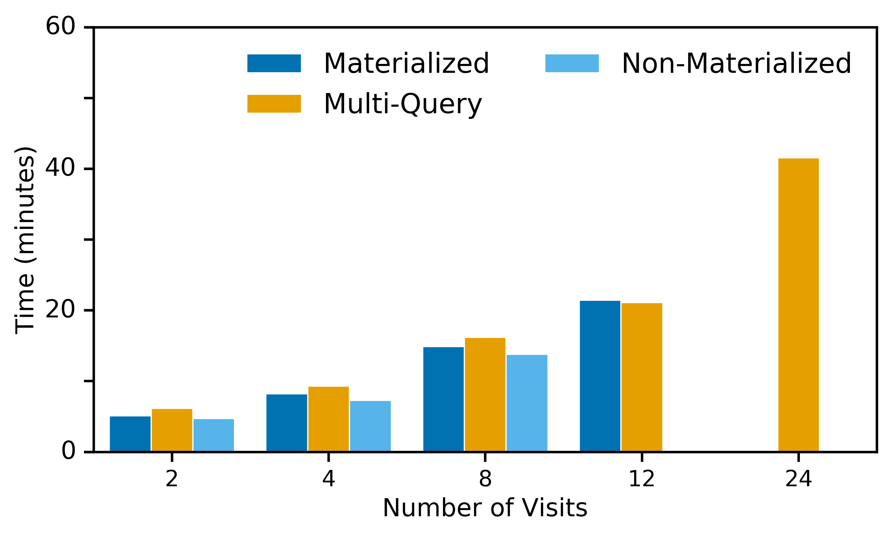
Figure 15: Execution time for the astronomy use case on Myria using different memory management techniques.

In TensorFlow, we executed one process per machine. For most operations, data conversions rather than other resources were the bottleneck eliminating the need for additional tuning. For the denoising step, memory was the bottleneck, which required the assignment of one image volume per physical machine. For filtering, we experimented with assigning different numbers of image volumes at a time to different workers on different machines and found a factor of 2$\times$ difference in total runtime between different assignments. Dask does not come with any partitioning capability and we manually tuned the number of workers and data partitions similar to Spark. Dask’s work stealing automatically load balances across the machines, however, work-stealing did not need any tuning.

In SciDB, it is good practice [33] to run one instance per 1-2 CPU cores. The chunk size, however, is more difficult to tune, as we did not find a strong correlation between the overall performance and common system configurations. We thus estimated the optimal chunk size for each operation by running the application with the same data set but using different chunk sizes. For instance, in Step  _A we found that a chunk size of $[1000\times 1000]$ of the LSST images leads to the best performance. Chunk size $[500\times 500]$, for example, is 3$\times$ slower; Chunk sizes $[1500\times 1500]$ and $[2000\times 2000]$ are slower by 22% and 55%, respectively.

5.3.2 Memory Management

Image analytics workloads are memory intensive. As we showed earlier in 10(a), the input data for 25 subjects is more than 100GB in size. The largest intermediate dataset produced by the analysis pipeline is over 200GB in size. Similarly, 24 exposures in the astronomy dataset yield over 100GB in size and nearly 300GB during processing. Additionally, data allocation can be skewed across compute nodes. For example, the astronomy pipeline grows the data by 2.5$\times$ on average during processing, but some workers experience data growth of 6$\times$ due to skew. As a result, image analytics pipelines can easily experience out-of-memory failures. Big data systems can use different approaches to trade-off query execution time and memory consumption. We evaluate some of these trade-offs in this section. In particular, we compare the performance of pipelined and materialized query execution. For materialized query execution, we compare materializing intermediate results and processing subsets of the input data at a time. Figure 15 shows the results for the Myria system on the astronomy use case. As the figure shows, when data is small compared with the available memory, the fastest way to execute the query is to pipeline intermediate results from one operator to the next. This approach is 8-11% faster in this experiment than materialization and 15-23% faster than executing multiple queries. As the ratio of data-to-memory grows, pipelining may cause a query to fail with an out-of-memory error. Intermediate result materialization then becomes the fastest query execution method. With even more data, the system must cut the data analysis into even smaller pieces for execution without failure.

In contrast to Myria, Spark can spill intermediate results to disk to avoid out-of-memory failures. Additionally, as we discussed in Section 5.3.1, Spark can partition data into smaller fragments than the number of available nodes, and will process only as many fragments as there are available slots. Both techniques help to avoid out-of-memory failures. However, this approach also causes Spark to be slower than Myria when memory is plentiful as shown earlier in 10(h).

5.3.3 Data Caching

Spark supports caching data in memory. Intermediate results replace the input data in memory as the computation proceeds and unless data is specifically cached a branch in the computation graph may result in re-computation of intermediate data. Caching can be harmful if the results are not needed by multiple steps as caching reduces the memory available to query processing. In our use cases, opportunities for data reuse are limited. Nevertheless, we found that caching the input data for the neuroscience use case yielded a consistent 7-8% runtime improvement across input data sizes.

6 Summary and Future Work

Our experiments have shown that while all of the evaluated systems have their strengths and weaknesses, none of them serves all the needs of large-scale image analytics. We summarize our key lessons learned:

User Defined Functions: Supporting user defined functions written in the language favored by scientists is an important requirement of large-scale image analytics. Scientists have legacy code that they seek to port and extend. Rewriting such computation using the domain-specific language provided by big data systems (e.g., SQL, AFL, etc.) is non-trivial, error-prone, and sometimes impossible when required functions (e.g., multidimensional convolution) are missing. Dask, Spark, and Myria were easier to use because of their flexible support for user-defined code in Python. SciDB’s stream() interface is an exciting new development in this regard.

Data Partitioning: When porting an existing image analytics pipeline to a big data system, the user must specify how to partition data across the cluster before invoking legacy, user-defined operations on the data. One challenge is that reference implementations do not indicate how computation can be parallelized. For example, Model building Step  _N processes the data for each voxel independently, but this independence is not evident from the reference implementation. In other cases, the reference implementation does not support parallelism even though the algorithm permits it. For example, Step  _A processes entire exposures even though only subsets of pixels are used to create each patch. An interesting area for future work is to enable support for legacy user code for parallel image analytics that does not require manual specification nor tuning of the data partitioning at each step.

Data Formats: Our evaluation shows the need for supporting user-defined functions but it also shows the performance of native operation implementations. A key challenge lies in data format transformations between the two types of operations. Predefined operations in big data systems work with internal formats (e.g., SciDB arrays, Myria relations, TensorFlow tensors) but user-defined functions use language- or domain-specific formats (e.g., NumPy arrays or FITS files). Conversions between formats adds overhead and complicates implementations. An interesting area of future work is to optimize away these format conversions.

System Tuning: All systems needed tuning, and none of them performed best with the default settings. System tuning, however, requires a deeper understanding of each of the systems, which is beyond the knowledge that should be required from users. Self-tuning thus remains an important goal for big data systems.

7 Related Work

Traditionally, image processing research has focused on effective indexing and querying of mutli-media content [9, 5, 6]. These systems focus on utilizing image content to create indices using attributes like color, texture, shape of image objects, and regions and then specifying similarity measures for querying, joining, etc.

There have been many benchmarks proposed by the DBMS community over the years such as the TPC benchmarks [38]. These benchmarks, however, focus on traditional Business Intelligence computations over structured data. Recently, the GenBase benchmark [36] took this forward to focus on complex analytics besides data management tasks, but did not examine image data. Pavlo et al., [28] evaluated the performance of MapReduce systems against parallel databases, but the analysis was limited to specific text analytic queries, not image analysis.

Several big data systems ([11, 19, 14, 30]) with similar capabilities to the ones we evaluated are available for large scale data analysis. We picked five representative systems that cover today’s key processing paradigms. We considered Rasdaman [30], which is an array database with capabilities similar to SciDB, but were unable to make much progress as the community version does not support UDFs.

8 Conclusion

We presented the first comprehensive study of large-scale image analytics on big data systems. We surveyed the major paradigms of large-scale data processing platforms using two real-world use cases from domain sciences. Our analysis shows that while we were able to execute the use-cases on several systems, leveraging the benefits of all systems required deep technical expertise. As such, we argue that current systems exhibit significant opportunities for further improvement and future research.

9 Acknowledgements

This project is supported in part by the National Science Foundation through NSF grants IIS-1247469, IIS-1110370, IIS-1546083, AST-1409547 and CNS-1563788; DARPA award FA8750-16-2-0032; DOE award DE-SC0016260, DE-SC0011635, and from the DIRAC Institute, gifts from Amazon, Adobe, Google, the Intel Science and Technology Center for Big Data, award from the Gordon and Betty Moore Foundation and the Alfred P Sloan Foundation, and the Washington Research Foundation Fund for Innovation in Data-Intensive Discovery.

References

- [1] M. Abadi et al. TensorFlow: Large-scale machine learning on heterogeneous systems, 2015.
- [2] ABCDSTUDY: Adolescent Brain Cognitive Development. http://abcdstudy.org/.
- [3] P. J. Basser, J. Mattiello, and D. LeBihan. Estimation of the effective self-diffusion tensor from the NMR spin echo. J. Magn. Reson. B, 103(3):247–254, Mar. 1994.
- [4] P. G. Brown. Overview of scidb: Large scale array storage, processing and analysis. In SIGMOD, SIGMOD ’10, pages 963–968, New York, NY, USA, 2010. ACM.
- [5] C. Carson et al. Blobworld: A system for region-based image indexing and retrieval. In VISUAL, pages 509–516, 1999.
- [6] S. Chaudhuri, L. Gravano, and A. Marian. Optimizing top-k selection queries over multimedia repositories. IEEE Trans. Knowl. Data Eng., 16(8):992–1009, 2004.
- [7] P. Coupe, P. Yger, S. Prima, P. Hellier, C. Kervrann, and C. Barillot. An optimized blockwise nonlocal means denoising filter for 3-D magnetic resonance images. IEEE Trans. Med. Imaging, 27(4):425–441, Apr. 2008.
- [8] Dask Development Team. Dask: Library for dynamic task scheduling. http://dask.pydata.org, 2016.
- [9] C. Faloutsos et al. Efficient and effective querying by image content. J. Intell. Inf. Syst., 3(3/4):231–262, 1994.
- [10] FITS: the astronomical image and table format. http://fits.gsfc.nasa.gov.
- [11] Apache Flink. https://flink.apache.org/.
- [12] The Fourth Paradigm: Data-Intensive Scientific Discovery. https://www.microsoft.com/en-us/research/publication/fourth-paradigm-data-intensive-scientific-discovery/.
- [13] E. Garyfallidis et al. Dipy, a library for the analysis of diffusion MRI data. Front. Neuroinform., 8:8, 21 Feb. 2014.
- [14] Apache Hadoop. http://hadoop.apache.org/.
- [15] D. Halperin et al. Demonstration of the myria big data management service. In SIGMOD, pages 881–884, 2014.
- [16] The High cadence Transient Survey (HiTS). http://astroinf.cmm.uchile.cl/category/projects/.
- [17] Big Data Strikes Back. https://medium.com/data-collective/rapid-growth-in-available-data-c5e2705a2423.
- [18] The Growth of Image Data: Mobile and Web. http://blog.d8a.com/post/9662265140/the-growth-of-image-data-mobile-and-web.
- [19] Apache Impala. http://impala.apache.org/.
- [20] T. L. Jernigan et al. The pediatric imaging, neurocognition, and genetics (ping) data repository. Neuroimage, 124:1149–1154, 2016.
- [21] N. Ji, J. Freeman, and S. L. Smith. Technologies for imaging neural activity in large volumes. Nat. Neurosci., 19(9):1154–1164, Aug. 2016.
- [22] Large Synoptic Survey Telescope. https://www.lsst.org/.
- [23] LSST Data Management. http://dm.lsst.org/.
- [24] K. L. Miller et al. Multimodal population brain imaging in the uk biobank prospective epidemiological study. Nature Neuroscience, 2016.
- [25] NiBabel: Access a cacophony of neuro-imaging file formats. http://nipy.org/nibabel/.
- [26] NIfTI: Neuroimaging informatics technology initiative. http://www.tpc.org.
- [27] N. Otsu. A threshold selection method from gray-level histograms. Automatica, 11(285-296):23–27, 1975.
- [28] A. Pavlo et al. A comparison of approaches to large-scale data analysis. In SIGMOD, pages 165–178, 2009.
- [29] PostgreSQL. https://www.postgresql.org/.
- [30] Rasdaman:raster data manager. http://www.rasdaman.org/.
- [31] M. Rocklin. Dask: Parallel computation with blocked algorithms and task scheduling. In K. Huff and J. Bergstra, editors, Proceedings of the 14th Python in Science Conference, pages 130 – 136, 2015.
- [32] SciDB. http://www.scidb.org/.
- [33] Paradigm4 forum. http://forum.paradigm4.com/t/persistenting-data-to-remote-nodes/1408/8.
- [34] E. Soroush et al. Efficient iterative processing in the scidb parallel array engine. In SSDBM, SSDBM ’15, pages 39:1–39:6, 2015.
- [35] Apache Spark. http://spark.apache.org/.
- [36] R. Taft, M. Vartak, N. R. Satish, N. Sundaram, S. Madden, and M. Stonebraker. Genbase: a complex analytics genomics benchmark. In SIGMOD, pages 177–188, 2014.
- [37] The Dark Energy Survey Collaboration. The Dark Energy Survey. ArXiv Astrophysics e-prints, Oct. 2005.
- [38] Tpc transaction processing performance council. https://nifti.nimh.nih.gov/nifti-1.
- [39] D. C. Van Essen, S. M. Smith, D. M. Barch, T. E. J. Behrens, E. Yacoub, K. Ugurbil, and WU-Minn HCP Consortium. The WU-Minn human connectome project: an overview. Neuroimage, 80:62–79, 15 Oct. 2013.
- [40] B. A. Wandell. Clarifying human white matter. Annu. Rev. Neurosci., 1 Apr. 2016.
- [41] J. Wang et al. The myria big data management and analytics system and cloud service. 2017.
- [42] M. Zaharia et al. Resilient distributed datasets: A fault-tolerant abstraction for in-memory cluster computing. In NSDI, pages 15–28, 2012.