Examples of computation of exact moment dynamics
for chemical reaction networks

Abstract

We review in a unified way results for two types of stochastic chemical reaction systems for which moments can be effectively computed:

1. feedforward networks (FFN), treated in [9], and

2. complex-balanced networks (CBN), treated in [10],

and provide several worked examples.

1 Stochastic Kinetics

We start by reviewing standard concepts regarding master equations for biochemical networks, see for instance [8].

1.1 Chemical Reaction Networks

Chemical reaction networks involve interactions among a finite set of species

$${\cal S}=\{S_{i},\,i=1,2,\ldots n\}$$

where one thinks of the $S_{i}$’s as counting the numbers of molecules of a certain type (or individuals in an ecological model, or cells in a cell population model):

$$S_{i}(t)=k_{i}=\mbox{ number of units of species }i\mbox{ at time }t\,.$$

In stochastic models, one thinks of these as random variables, which interact with each other. The complete vector $S=(S_{1},\ldots,S_{n})^{\prime}$ is called the state of the system at time $t$, and it is probabilistically described as a Markov stochastic process which is indexed by time $t\geq 0$ and takes values in ${\mathbb{Z}}_{\geq 0}^{n}$. Thus, $S(t)$ is a ${\mathbb{Z}}_{\geq 0}^{n}$-valued random variable, for each $t\geq 0$. (Abusing notation, we also write $S(t)$ to represent an outcome of this random variable on a realization of the process.) We will denote

$$p_{k}(t)={\mathbb{P}}\,{\left[S(t)=k\right]}$$

for each $k\in{\mathbb{Z}}_{\geq 0}^{n}$. Then $p(t)=(p_{k})_{k\in{\mathbb{Z}}_{\geq 0}^{n}}$ is the discrete probability density (also called the “probability mass function”) of $S(t)$. To describe the Markov process, one needs to formally introduce chemical reaction networks.

Mathematically, a chemical reaction network is a finite set

$${\cal R}=\{R_{j},j=1,2,\ldots,m\}$$

of formal transformations or reactions

$$R_{j}:\quad\sum_{{i}=1}^{n}a_{{i}{j}}S_{i}\;\longrightarrow\;\sum_{{i}=1}^{n}b_{{i}{j}}S_{i}\,,\quad j\in\{1,2,\ldots,m\}$$ (1)

among species, together with a set of $m$ functions

$$\rho_{j}:{\mathbb{Z}}_{\geq 0}^{n}\rightarrow{\mathbb{R}}_{\geq 0},\quad{j}=1,\ldots,m,\mbox{ with }\rho_{j}(0)=0$$

called the propensity functions for the respective reactions $R_{j}$. The coefficients $a_{{i}{j}}$ and $b_{{i}{j}}$ are non-negative integers, called the stoichiometry coefficients, and the sums are understood informally, indicating combinations of elements. The intuitive interpretation is that $\rho_{j}(S_{1},\ldots,S_{n})dt$ is the probability that reaction $R_{j}$ takes place, in a short interval of length $dt$, provided that the complete state was $S=(S_{1},\ldots,S_{n})$ at the beginning of the interval. In principle, the propensities can be quite arbitrary functions, but we will focus on mass-action kinetics, for which the functions $\rho_{j}$ are polynomials whose degree is the sum of the $a_{{i}{j}}$’s in the respective reaction. Before discussing propensities, however, we need to introduce some more notations and terminology.

The linear combinations $\sum_{{i}=1}^{n}a_{{i}{j}}S_{i}$ and $\sum_{{i}=1}^{n}b_{{i}{j}}S_{i}$ appearing in the $m$ reactions are called the complexes involved in the reactions. For each reaction $R_{j}$, we collect the coefficients appearing on its left-hand side and on its right-hand side into two vectors, respectively:

$${\mathbb{S}}(R_{j})=a_{j}:=(a_{1{j}},\ldots,a_{n{j}})^{\prime}\,,\quad{\mathbb{T}}(R_{j})=b_{j}:=(b_{1{j}},\ldots,b_{n{j}})^{\prime}$$

(prime indicates transpose). We call ${\mathbb{S}},{\mathbb{T}}:{\cal R}\rightarrow{\cal C}$ the source and target functions, where ${\cal C}\subseteq{\mathbb{Z}}^{n}_{\geq 0}$ is the set of all vectors $\left\{a_{j},b_{j},j=1\ldots m\right\}$. We identify complexes with elements of ${\cal C}$. The reactants $S_{i}$ of the reaction $R_{j}$ are those species appearing with a nonzero coefficient, $a_{{i}{j}}\not=0$ in its left-hand side and the products $S_{i}$ of reaction $R_{j}$ are those species appearing with a nonzero coefficient $b_{{i}{j}}\not=0$ in its right-hand side.

For every vector of non-negative integers $v=(v_{1},\ldots,v_{n})\in{\mathbb{Z}}_{\geq 0}^{n}$, let us write the sum of its entries as $\oplus v:=v_{1}+\ldots+v_{n}$. In particular, for each $j\in\{1,\ldots,m\}$, we define the order of the reaction $R_{j}$ as $\oplus a_{j}:=\,\sum_{{i}=1}^{n}a_{{i}{j}}$, which is the total number of units of all species participating in the reaction $R_{j}$.

The $n\times m$ stoichiometry matrix $\Gamma=\{\gamma_{{i}{j}}\}$ is defined as the matrix whose entries are defined as follows:

$$\gamma_{{i}{j}}:=\,b_{{i}{j}}-a_{{i}{j}}\,,\quad{i}=1,\ldots,n,\;{j}=1,\ldots,m\,.$$

The integer $\gamma_{{i}{j}}$ counts the net change (positive or negative) in the number of units of species $S_{i}$ each time that the reaction $R_{j}$ takes place. We will denote by $\gamma_{j}$ the ${j}$th column of $\Gamma$. Note that, with the notations introduced so far,

$$\gamma_{j}\,=\,b_{j}-a_{j}\,,\quad{j}=1,\ldots,m\,.$$

We will assume, to avoid trivial situations, that $\gamma_{j}\not=0$ for all $j$ (that is, each reaction changes at least some species).

For example, suppose that $n=4$, $m=2$, and the reactions are

$$R_{1}:\,S_{1}+S_{2}\,\rightarrow\,S_{3}+S_{4}\,,\;\;\;R_{2}:\,2S_{1}+S_{3}\,\rightarrow\,S_{2}$$

which have orders $1+1=2$ and $2+1=3$ respectively. The set ${\cal C}$ has four elements, which list the coefficients of the species participating in the reactions:

$${\cal C}=\{(1,1,0,0)^{\prime},(0,0,1,1)^{\prime},(2,0,1,0)^{\prime},(0,1,0,0)^{\prime}\}$$

with

$${\mathbb{S}}(R_{1})=a_{1}=(1,1,0,0)^{\prime},\,{\mathbb{S}}(R_{2})=a_{2}=(2,0,1,0)^{\prime},\,{\mathbb{T}}(R_{1})=b_{1}=(0,0,1,1)^{\prime},\,{\mathbb{T}}(R_{1})=b_{2}=(0,1,0,0)^{\prime}$$

and $\gamma_{1}=(-1,-1,1,1)^{\prime}$, $\gamma_{2}=(-2,1,-1,0)^{\prime}$. The reactants of $R_{1}$ are $S_{1}$ and $S_{2}$, the reactants of $R_{2}$ are $S_{1}$ and $S_{3}$, the products of $R_{1}$ are $S_{3}$ and $S_{4}$, the only product of $R_{2}$ is $S_{2}$, and the stoichiometry matrix is

$$\Gamma\;=\;\left(\begin{array}[]{cccccccccccc}-1&-2\cr-1&1\cr 1&-1\cr 1&0\end{array}\right)\,.$$

It is sometimes convenient to write

$$\sum_{{i}=1}^{n}a_{{i}{j}}S_{i}\;\xrightarrow{\rho_{j}(S)}\;\sum_{{i}=1}^{n}b_{{i}{j}}S_{i}$$

to show that the propensity $\rho_{j}$ is associated to the reaction $j$, and also to combine two reactions $R_{j}$ and $R_{k}$ that are the reverse of each other, meaning that their complexes are transposed: ${\mathbb{S}}(R_{j})={\mathbb{T}}(R_{k})$ and ${\mathbb{S}}(R_{k})={\mathbb{T}}(R_{j})$, by using double arrows, like

$$\sum_{{i}=1}^{n}a_{{i}{j}}S_{i}\;\xrightleftharpoons[\rho_{k}(S)]{\rho_{j}(S)}\;\sum_{{i}=1}^{n}b_{{i}{j}}S_{i}\,.$$

When propensities are given by mass-action kinetics, as discussed below, one simply writes on the arrows the kinetic constants instead of the full form of the kinetics.

1.2 Chemical Master Equation

A Chemical Master Equation (CME), which is the differential form of the Chapman-Kolmogorov forward equation is a system of linear differential equations that describes the time evolution of the joint probability distribution of the $S_{i}(t)$’s:

$$\frac{dp_{k}}{dt}\;=\;\sum_{{j}=1}^{m}\rho_{j}(k-\gamma_{j})\,p_{k-\gamma_{j}}-\sum_{{j}=1}^{m}\rho_{j}(k)\,p_{k}\,,\quad k\in{\mathbb{Z}}_{\geq 0}^{n}$$ (2)

where, for notational simplicity, we omitted the time argument “$t$” from $p$, and the function $\rho_{j}$ has the property that $\rho_{j}(k-\gamma_{j})=0$ unless $k\geq\gamma_{j}$ (coordinatewise inequality). There is one equation for each $k\in{\mathbb{Z}}_{\geq 0}^{n}$, so this is an infinite system of linked equations. When discussing the CME, we will assume that an initial probability vector $p(0)$ has been specified, and that there is a unique solution of (2) defined for all $t\geq 0$. (See [7] for existence and uniqueness results.) A different CME results for each choice of propensity functions, a choice that is dictated by physical chemistry considerations.

The most commonly used propensity functions, and the ones best-justified from elementary physical principles, are ideal mass action kinetics propensities, defined as follows (see [4]), proportional to the number of ways in which species can combine to form the $j$th source complex:

$$\rho_{j}(k)=\kappa_{j}\prod_{{i}=1}^{n}{k_{i}\choose a_{{i}{j}}}\,{\cal H}(k-a_{{j}})\,\quad{j}=1,\ldots,m.$$ (3)

where, for any scalar or vector, we denote ${\cal H}(u)=1$ if $u\geq 0$ (coordinatewise) and ${\cal H}(u)=0$ otherwise. In other words, the expression can only be nonzero provided that $k_{i}\geq a_{{i}{j}}$ for all $i=1,\ldots,n$ (and thus the combinatorial coefficients are well-defined). Observe that the expression in the right-hand side makes sense even if $k\ngeq 0$, in the following sense. In that case, $k_{i}<0$ for some index $i$, so the factorial is not well-defined, but on the other hand, $k_{i}-a_{{i}{j}}\leq k_{i}<0$ implies that ${\cal H}(k-a_{{j}})=0$. So $\rho_{j}(k)$ can be thought of as defined by this formula for all $k\in{\mathbb{Z}}^{n}$, even if some entries of $k$ are negative, but is zero unless $k\geq 0$, and the combinatorial coefficients can be arbitrarily defined for $k\ngeq 0$. (In particular, $\rho_{j}(k-\gamma_{j})=0$ unless $k\geq\gamma_{j}$ in (2).) The $m$ non-negative “kinetic constants” are arbitrary, and they represent quantities related to the volume, shapes of the reactants, chemical and physical information, and temperature. The model described here assumes that temperature and volume are constant, and that the system is well-mixed (no spatial heterogeneity).

1.3 Derivatives of moments expressed as linear combinations of moments

Notice that $\rho_{j}(k)$ can be expanded into a polynomial in which each variable $k_{i}$ has an exponent less or equal to $a_{ij}$. In other words,

$$\rho_{j}(k)=\sum_{c_{j}\leq a_{j}}\kappa_{c_{j}}\,k^{c_{j}}$$

(“$\leq$” is understood coordinatewise, and by definition $k^{c_{j}}=k_{1}^{c_{1j}}\ldots k_{n}^{c_{nj}}$ and $r^{0}=1$ for all integers), for suitably redefined coefficients $\kappa_{c_{j}}$’s.

Suppose given a function $M:{\mathbb{Z}}_{\geq 0}^{n}\rightarrow{\mathbb{R}}$ (to be taken as a monomial when computing moments). The expectation of the random variable $M(S)$ is by definition

$${\mathbb{E}}\left[M(S(t))\right]=\sum_{k\in{\mathbb{Z}}_{\geq 0}^{n}}p_{k}(t)\,M(k)\,,$$

since $p_{k}(t)={\mathbb{P}}\,{\left[S(t)=k\right]}$. Let us define, for any $\gamma\in{\mathbb{Z}}^{n}$, the new function $\Delta_{\gamma}M$ given by

$$(\Delta_{\gamma}M)(k):=M(k+\gamma)-M(k)\,.$$

With these notations,

$$\frac{d}{dt}{\mathbb{E}}\left[M(S(t))\right]\;=\;\sum_{j=1}^{m}{\mathbb{E}}\left[\rho_{j}(S(t))\,\Delta_{\gamma_{j}}M(S(t))\right]$$ (4)

(see [8] for more details). We next specialize to a monomial function:

$$M(k)=k^{u}=k_{1}^{u_{1}}k_{2}^{u_{2}}\ldots k_{n}^{u_{n}}$$

where $u\in{\mathbb{Z}}_{\geq 0}^{n}$. There results

$$(\Delta_{\gamma_{j}}M)(k)=\sum_{\nu\in{\cal I}(u,j)}\,d_{\nu}k^{\nu}$$

for appropriate coefficients $d_{\nu}$, where

$${\cal I}(u,j):=\left\{\nu\in{\mathbb{Z}}_{\geq 0}^{n}\left|\begin{aligned} &\nu=u-\mu,\;u\geq\mu\not=0\\ \mu_{i}=0&\mbox{ for each }i\mbox{ such that }\gamma_{{i}{j}}=0\end{aligned}\right.\right\}$$

(inequalities “$\geq$” in ${\mathbb{Z}}_{\geq 0}^{n}$ are understood coordinatewise). Thus, for (3):

$$\frac{d}{dt}{\mathbb{E}}\left[S(t)^{u}\right]=\sum_{j=1}^{m}\,\sum_{c_{j}\leq a_{j}}\,\sum_{\nu\in{\cal I}(u,j)}d_{\nu}\kappa_{c_{j}}\,{\mathbb{E}}\left[S(t)^{\nu+c_{j}}\right].$$ (5)

In other words, we can recursively express the derivative of the moment of order $u$ as a linear combination of other moments. This results in an infinite set of coupled linear ordinary differential equations, so it is natural to ask whether, for given a particular moment or order $u$ of interest, there is a finite set of moments, including the desired one, that satisfies a finite set of differential equations. This question can be reformulated combinatorially, as follows.

For each multi-index $u\in{\mathbb{Z}}_{\geq 0}^{n}$, let us define ${\cal R}^{0}(u)=\{u\}$,

$${\cal R}^{1}(u)\,:=\;\left\{\nu+c_{j}\,,\;1\leq j\leq m,c_{j}\leq a_{j},\,\nu\in{\cal I}(u,j)\right\}$$

and, more generally, for any $\ell\geq 1$,

$${\cal R}^{\ell+1}(u)\,:=\;{\cal R}^{1}({\cal R}^{\ell}(u))$$

where, for any set $U$, ${\cal R}^{\ell}(U):=\bigcup_{u\in U}{\cal R}^{\ell}(u)$. Finally, we set

$${\cal R}(u)\,:=\;\bigcup_{i=0}^{\infty}{\cal R}^{i}(u).$$

Each set ${\cal R}^{\ell}(u)$ is finite, but the cardinality $\#({\cal R}(u))$ may be infinite. It is finite if and only if there is some $L\geq 0$ such that ${\cal R}(u)=\bigcup_{i=0}^{L}{\cal R}^{i}(u)$, or equivalently ${\cal R}^{L+1}(u)\subseteq\bigcup_{i=0}^{L}{\cal R}^{i}(u)$.

Equation (5) says that the derivative of the $u$-th moment can be expressed as a linear combination of the moments in the set ${\cal R}^{1}(u)$. The derivatives of these moments, in turn, can be expressed in terms of the moments in the set ${\cal R}^{1}(u^{\prime})$, for each $u^{\prime}\in{\cal R}^{1}(u)$, i.e., in terms of moments in the set ${\cal R}^{2}(u)$. Iterating, we have the following: “Finite reachability implies linear moment closure” observation:

Lemma. Suppose that $N:=\#({\cal R}(u))<\infty$, and ${\cal R}(u)=\{u=u_{1},\ldots,u_{N}\}$. Then, writing

$$x(t):=\left({\mathbb{E}}\left[S^{u_{1}}(t)\right],\ldots,{\mathbb{E}}\left[S^{u_{N}}(t)\right]\right)^{\prime},$$

there is an $A\in{\mathbb{R}}^{N\times N}$ such that $\dot{x}(t)=Ax(t)$ for all $t\geq 0$.

A classical case is that in which all reactions have order 0 or 1, i.e. $\oplus a_{j}\in\{0,1\}$. Indeed, since $\mu\not=0$ in the definition of ${\cal I}(u,j)$, it follows that $\oplus a_{j}\leq\oplus\mu$ for every index $j$. Therefore, $\oplus(\nu+a_{j})=\oplus u+\oplus a_{j}-\oplus\mu\leq\oplus u$ for all $u$, and the same holds for $\nu+c_{j}$ if $c_{j}\leq a_{j}$. So all elements in ${\cal R}(u)$ have degree $\leq\oplus u$, and thus $\#({\cal R}(u))<\infty$. A more general case is as follows.

2 Feedforward networks

A chemical network will be said to be of feedforward type (FFN) if one can partition its $n$ species

$$S_{i}\,,\quad i\in\{1,2,\ldots,n\}$$

into $p$ layers

$$\mathbf{S}_{1},\ldots,\mathbf{S}_{p}$$

and there are a total of $m^{\prime}=m+d$ reactions, where $d$ of the reactions are “pure degradation” (or “dilution”) reactions

$$D_{j}:S_{i_{j}}\rightarrow 0\,,\quad j\in\{1,\ldots,d\}$$

and the additional $m$ reactions

$$R_{j}\,,\quad j\in\{1,2,\ldots,m\}$$

can be partitioned into $p\geq 1$ layers

$$\mathbf{R}_{1},\ldots,\mathbf{R}_{p}$$

in such a manner that, in the each reaction layer $R_{\pi}$ there may be any number of order-zero or order-one reactions involving species in layer $\pi$, but every higher-order reaction at a layer $\pi>1$ must have the form:

$$a_{{i_{1}}{j}}S_{{i_{1}}}+\ldots a_{{i_{q}}{j}}S_{{i_{q}}}\quad\longrightarrow\quad a_{{i_{1}}{j}}S_{{i_{1}}}+\ldots a_{{i_{q}}{j}}S_{{i_{q}}}+b_{{i_{q+1}}{j}}S_{{i_{q+1}}}+\ldots b_{{i_{q+q^{\prime}}}{j}}S_{{i_{q+q^{\prime}}}}$$

where all the species $S_{{i_{1}}},\ldots,S_{{i_{q}}}$ belong to layers having indices $<\pi$, and the species $S_{{i_{q+1}}},\ldots,S_{{i_{q+q^{\prime}}}}$ are in layer $\pi$. In other words, multimers of species in “previous” layers can “catalyze” the production of species in the given layer, but are not affected by these reactions. This can be summarized by saying that for reactions at any given layer $\pi$, the only species that appear as reactants in nonlinear reactions are those in layers $<\pi$ and the only ones that can change are those in layer $\pi$.

A more formal way to state the requirements is as follows. The reactions $R_{j}$ that belong to the first layer $\mathbf{R}_{1}$ are all of order zero or one, i.e. they have $\oplus a_{j}\in\{0,1\}$ (this first layer might model several independent separate chemical subnetworks; we collect them all as one larger network), and

$$\mbox{if }R_{j}\in\mathbf{R}_{\pi}:\left\{\begin{array}[]{ll}a_{{i}{j}}\not=0\mbox{ and }\oplus a_{j}>1&\Rightarrow S_{i}\in\bigcup_{1\leq s<\pi}\mathbf{S}_{\pi}\\ \gamma_{{i}{j}}\not=0&\Rightarrow S_{i}\in\mathbf{S}_{\pi}\,.\end{array}\right.$$ (6)

It was shown in [9] that FFN’s have the finite reachability property: given any desired moment $u$, there is a linear differential equation $\dot{x}(t)=Ax(t)$ for a suitable set of $N$ moments

$$x(t):=\left({\mathbb{E}}\left[S^{u_{1}}(t)\right],\ldots,{\mathbb{E}}\left[S^{u_{N}}(t)\right]\right)^{\prime},$$

which contains the moment $u$ of interest. Notice that steady-state moments can then be computed by solving $Ax=0$.

In practice, we simply compute (5) starting from a desired moment, then recursively apply the same rule to the moments appearing in the right-hand side, and so forth until no new moments appear. The integer $N$ at which the system closes might be very large, but the procedure is guaranteed to stop.

We also remark that the last section of the paper [9] explains how certain non-feedforward networks also lead to moment closure, provided that conservation laws ensure that variables appearing ion nonlinear reactions take only a finite set of possible values. We do not discuss that case here.

2.1 Steady-states of CME

Often, the interest is in long-time behavior, after a transient, that is to say in the probabilistic steady state of the system: the joint distribution of the random variables $S_{i}=S_{i}(\infty)$ that result in the limit as $t\rightarrow\infty$ (provided that such a limit exists in an appropriate technical sense). This joint distribution is a solution of the steady state CME (ssCME), the infinite set of linear equations obtained by setting the right-hand side of the CME to zero, that is:

$$\sum_{{j}=1}^{m}\rho_{j}(k-\gamma_{j})\,p_{k-\gamma_{j}}\;=\;\sum_{{j}=1}^{m}\rho_{j}(k)\,p_{k}\,,\quad k\in{\mathbb{Z}}_{\geq 0}^{n}$$ (7)

with the convention that $\rho_{j}(k-\gamma_{j})=0$ unless $k\geq\gamma_{j}$. When substituting mass action propensities

$$\rho_{j}(k)=\kappa_{j}\prod_{{i}=1}^{n}{k_{i}\choose a_{{i}{j}}}\,{\cal H}(k-a_{{j}})$$

the steady-state equation (7) becomes:

$$\sum_{{j}=1}^{m}\,\kappa_{j}\,\prod_{{i}=1}^{n}{k_{i}-\gamma_{ij}\choose a_{{i}{j}}}\,{\cal H}(k-b_{j})\,p_{k-\gamma_{j}}\;=\;\sum_{{j}=1}^{m}\,\kappa_{j}\,\prod_{{i}=1}^{n}{k_{i}\choose a_{{i}{j}}}\,{\cal H}(k-a_{{j}})\,p_{k}\,,\quad k\in{\mathbb{Z}}_{\geq 0}^{n}\,.$$ (8)

Equivalently,

$$\sum_{{j}=1}^{m}\,{\widetilde{\kappa}}_{j}\,\prod_{{i}=1}^{n}\frac{\left(k_{i}-\gamma_{ij}\right)!}{\left(k_{i}-b_{{i}{j}}\right)!}\,{\cal H}(k-b_{j})\,p_{k-\gamma_{j}}\;=\;\sum_{j=1}^{m}\,{\widetilde{\kappa}}_{j}\,\prod_{{i}=1}^{n}\frac{k_{i}!}{\left(k_{i}-a_{{i}{j}}\right)!}\,{\cal H}(k-a_{{j}})\,p_{k}\,,\quad k\in{\mathbb{Z}}_{\geq 0}^{n}$$ (9)

when introducing the new constants ${\widetilde{\kappa}}_{j}:={\kappa_{j}}/{\prod_{{i}=1}^{n}\left(a_{{i}{j}}!\right)}$. If, for convenience, we write:

$${\lambda}^{k}\,:=\;\lambda_{1}^{k_{1}}\ldots\lambda_{n}^{k_{n}}\quad\mbox{and}\quad k!\,:=\;k_{1}!\ldots k_{n}!$$

for each nonnegative integer vector $k=(k_{1},\ldots,k_{n})\in{\mathbb{Z}}_{\geq 0}^{n}$ and positive vector $\lambda=(\lambda_{1},\ldots,\lambda_{n})\in{\mathbb{R}}_{>0}^{n}$, then (10) is re-written as

$$\sum_{{j}=1}^{m}\,{\widetilde{\kappa}}_{j}\,\frac{\left(k-\gamma_{j}\right)!}{\left(k-b_{j}\right)!}\,{\cal H}(k-b_{j})\,p_{k-\gamma_{j}}\;\;=\;\;\sum_{{j}=1}^{m}\,{\widetilde{\kappa}}_{j}\,\frac{k!}{\left(k-a_{j}\right)!}\,{\cal H}(k-a_{{j}})\,p_{k}\,,\quad k\in{\mathbb{Z}}_{\geq 0}^{n}$$ (10)

Since (10) is a linear equation on the $\left\{p_{k},k\in{\mathbb{Z}}_{\geq 0}^{n}\right\}$, any rescaling of a given set of $p_{k}$’s will satisfy the same equation; for probability densities, one normalizes to a unit sum.

If there are conservation laws satisfied by the system then steady state solutions will not be unique, and the equation $Ax=0$ must be supplemented by a set of linear constraints that uniquely specify the solution. This is obvious even for simple linear reactions. For example, suppose we consider one reversible reaction

$$S_{1}\;\xrightleftharpoons[\kappa_{2}]{\kappa_{1}}\;S_{2}$$

(propensities are mass-action, $\rho_{i}(S_{1},S_{2})=\kappa_{i}S_{i}$). The first moments (means) satisfy $\dot{x}_{1}=\kappa_{2}x_{2}-\kappa_{1}x_{1}$ and $\dot{x}_{2}=\kappa_{1}x_{1}-\kappa_{2}x_{2}$. Any vector $({\bar{\xi}}_{1},{\bar{\xi}}_{2})$ with $\kappa_{1}{\bar{\xi}}_{1}=\kappa_{2}{\bar{\xi}}_{2}$ is a steady state of these equations. However, the sum of the numbers of molecules $S_{1}$ and $S_{2}$ is conserved in the reactions. Given a particular total number, $\beta$, the differential equations can be reduced to just one equation, say for $x_{1}$: $\dot{x}_{1}=\kappa_{2}(\beta-x_{1})-\kappa_{1}x_{1}=-(\kappa_{1}+\kappa_{2})x_{1}+\kappa_{2}\beta$, which has the affine form $\dot{x}=Ax+b$. At steady state, we have the unique solution ${\bar{\xi}}_{1}=\beta\kappa_{2}/(\kappa_{1}+\kappa_{2})$, ${\bar{\xi}}_{2}=\beta\kappa_{1}/(\kappa_{1}+\kappa_{2})$ obtained by imposing the constraint ${\bar{\xi}}_{1}+{\bar{\xi}}_{2}=\beta$. It can easily be proved (see e.g. [10]) that at steady state, $S_{1}$ is a binomial random variable $B(\beta,p)$ with $p=\frac{1}{1+\mu}$, where $\mu=\kappa_{1}/\kappa_{2}$. We later discuss further the effect of conservation laws.

2.2 A worked example

For networks with only zero and first order reactions, which are trivially in our feedforward class, it is well-known that one may compute all moments in closed form. We work out a simple example here. Again we start with a reversible reaction

$$S_{1}\;\xrightleftharpoons[\delta]{\kappa}\;S_{2}$$

and mass-action propensities. We think in this context of $S_{1}$ as the active form of a certain gene and $S_{2}$ as the inactive form of the same gene. Transcription and translation are summarized, for simplicity, as one reaction

$$S_{1}\;\xrightarrow{\rho}\;S_{1}+S_{3}$$

and degradation or dilution of the gene product $S_{3}$ is a linear reaction

$$S_{3}\;\xrightarrow{\eta}\;\emptyset\,.$$

The stoichiometry matrix is

$$\Gamma=\left(\begin{array}[]{cccccccccccc}-1&1&0&0\cr 1&-1&0&0\cr 0&0&1&-1\end{array}\right)\,.$$

Suppose that we are interested in the mean and variance of $S_{3}$ subject to the conservation law $S_{1}+S_{2}=\beta$, for some fixed positive integer $\beta$. A linear differential equation for the vector of second order moments:

$${\cal M}\;=\;(E[S_{1}],E[S_{1}^{2}],E[S_{1}S_{3}],E[S_{3}],E[S_{3}^{2}])^{\prime}$$

is $\dot{\cal M}=A{\cal M}+b$, where

$$A\;=\;\left(\begin{array}[]{ccccc}-\delta-\kappa&0&0&0&0\\ \kappa-\delta+2\,\delta\,\beta&-2\,\delta-2\,\kappa&0&0&0\\ 0&\rho&-\delta-\eta-\kappa&\delta\,\beta&0\\ \rho&0&0&-\eta&0\\ \rho&0&2\,\rho&\eta&-2\,\eta\end{array}\right)\;,\quad\quad b\;=\;\left(\begin{array}[]{c}\delta\,\beta\\ \delta\,\beta\\ 0\\ 0\\ 0\end{array}\right)$$

Solving $A\overline{{\cal M}}+b=0$ to obtain steady state moments, we have:

$$\overline{{\cal M}}\;=\;\left(\begin{array}[]{c}\frac{\delta\,\beta}{\delta+\kappa}\\ \frac{\delta\,\beta\,\left(\kappa+\delta\,\beta\right)}{{\left(\delta+\kappa\right)}^{2}}\\ \frac{\delta\,\beta\,\rho\,\left(\eta\,\kappa+{\delta}^{2}\,\beta+\delta\,\eta\,\beta+\delta\,\kappa\,\beta\right)}{\eta\,{\left(\delta+\kappa\right)}^{2}\,\left(\delta+\eta+\kappa\right)}\\ \frac{\delta\,\beta\,\rho}{\eta\,\left(\delta+\kappa\right)}\\ \frac{\delta\,\beta\,\rho\,\left({\delta}^{2}\,\eta+\beta\,\rho\,{\delta}^{2}+\delta\,{\eta}^{2}+2\,\delta\,\eta\,\kappa+\beta\,\rho\,\delta\,\eta+\beta\,\rho\,\delta\,\kappa+{\eta}^{2}\,\kappa+\eta\,{\kappa}^{2}+\rho\,\eta\,\kappa\right)}{{\eta}^{2}\,{\left(\delta+\kappa\right)}^{2}\,\left(\delta+\eta+\kappa\right)}\end{array}\right)\,.$$

2.3 A simple nonlinear example

We consider a feedforward system in which there are three species; $S_{1}$ catalyzes production $S_{2}$, and $S_{1}$ and $S_{2}$ are both needed to produce $S_{3}$:

$$0\xrightarrow{\kappa_{1}}S_{1}\xrightarrow{\delta_{1}}0\quad S_{1}\xrightarrow{\kappa_{2}}S_{1}+S_{2}\quad S_{2}\xrightarrow{\delta_{2}}0\quad S_{1}+S_{2}\xrightarrow{\kappa_{3}}S_{1}+S_{2}+S_{3}\quad S_{3}\xrightarrow{\delta_{3}}0$$

Computing $E[S_{3}]$, the mean of $S_{3}$, requires a minimal differential equation of order 5, for the moments

$${\cal M}\;=\;(E[S_{3}],E[S_{1}S_{2}],E[S_{2}],E[S_{1}^{2}],E[S_{1}])^{\prime}$$

and has form $\dot{\cal M}=A{\cal M}+b$, where

$$A=\left(\begin{array}[]{ccccc}-\delta_{2}&\kappa_{3}&0&0&0\\ 0&-\delta_{1}-\delta_{2}&\kappa_{1}&\kappa_{2}&0\\ 0&0&-\delta_{2}&0&\kappa_{2}\\ 0&0&0&-2\,\delta_{1}&2\,\kappa_{1}+\delta_{1}\\ 0&0&0&0&-\delta_{1}\end{array}\right)\quad\mbox{and}\quad b=\left(\begin{array}[]{c}0\\ 0\\ 0\\ \kappa_{1}\\ \kappa_{1}\end{array}\right)\,.$$

3 Poisson-like solutions and complex-balanced networks

We observe that for any given positive vector ${\bar{\lambda}}\in{\mathbb{R}}_{>0}^{n}$, the set of numbers

$$\Pi\,=\,\left\{p_{k}=\frac{{\bar{\lambda}}^{k}}{k!}\;,\;\;k\in{\mathbb{Z}}_{\geq 0}^{n}\right\}$$ (11)

satisfies the ssCME equations (10) if and only if

$$\sum_{{j}=1}^{m}\,{\widetilde{\kappa}}_{j}\,\frac{{\bar{\lambda}}^{k-\gamma_{j}}}{\left(k-b_{j}\right)!}\,{\cal H}(k-b_{j})\;\;=\;\;\sum_{{j}=1}^{m}\,{\widetilde{\kappa}}_{j}\,\frac{{\bar{\lambda}}^{k}}{\left(k-a_{j}\right)!}\,{\cal H}(k-a_{{j}})\,,\quad k\in{\mathbb{Z}}_{\geq 0}^{n}\,,$$ (12)

Re-writing this as:

$$\sum_{c\in{\cal C}}\sum_{\{j|b_{j}=c\}}\,{\widetilde{\kappa}}_{j}\,\frac{{\bar{\lambda}}^{k-\gamma_{j}}}{\left(k-b_{j}\right)!}\,{\cal H}(k-b_{j})\;\;=\;\;\sum_{c\in{\cal C}}\sum_{\{j|a_{j}=c\}}\,{\widetilde{\kappa}}_{j}\,\frac{{\bar{\lambda}}^{k}}{\left(k-c\right)!}\,{\cal H}(k-a_{{j}})\,,\quad k\in{\mathbb{Z}}_{\geq 0}^{n}\,,$$ (13)

we see that a sufficient condition for (11) to be a solution is that for each individual complex $c\in{\cal C}$:

$$\sum_{\{j|b_{j}=c\}}\,{\widetilde{\kappa}}_{j}\,\frac{{\bar{\lambda}}^{k-\gamma_{j}}}{\left(k-c\right)!}\,{\cal H}(k-b_{j})\;\;=\;\;\sum_{\{j|a_{j}=c\}}\,{\widetilde{\kappa}}_{j}\,\frac{{\bar{\lambda}}^{k}}{\left(k-c\right)!}\,{\cal H}(k-a_{{j}})\,,\quad k\in{\mathbb{Z}}_{\geq 0}^{n}\,,$$

or, equivalently,

$$\frac{{\cal H}(k-c)}{\left(k-c\right)!}\sum_{\{j|b_{j}=c\}}\,{\widetilde{\kappa}}_{j}\,{\bar{\lambda}}^{k-\gamma_{j}}\;\;=\;\;\frac{{\cal H}(k-c)}{\left(k-c\right)!}\sum_{\{j|a_{j}=c\}}\,{\widetilde{\kappa}}_{j}\,{\bar{\lambda}}^{k}\,,\quad k\in{\mathbb{Z}}_{\geq 0}^{n}\,.$$

A sufficient condition for this to hold is that

$$\sum_{\{j|b_{j}=c\}}\,{\widetilde{\kappa}}_{j}\,{\bar{\lambda}}^{a_{j}}\;\;=\;\;\sum_{\{j|a_{j}=c\}}\,{\widetilde{\kappa}}_{j}\,{\bar{\lambda}}^{a_{j}}\,,\quad k\in{\mathbb{Z}}_{\geq 0}^{n}$$ (14)

holds for all complexes (and conversely, this last condition is necessary for all complexes for which $k\geq c$). Note that one can equally well write “${{\bar{\lambda}}}^{c}$” and bring this term outside of the sum, in the right-hand side.

When property (14) holds for every complex, one says that ${\bar{\lambda}}$ is a complex balanced steady state of the associated deterministic chemical reaction network. (That is, the system of differential equations $\dot{x}=\Gamma Q(x)$, where $Q(x)$ is a column vector of size $m$ whose $j$th entry is $\rho_{j}(x)$ and $x(t)\in{\mathbb{R}}_{\geq 0}^{n}$ for all $t$.) Complex balancing means that, for each complex, outflows and inflows balance out. This is a Kirschoff current law (in-flux = out-flux, at each node). See Figure 1.

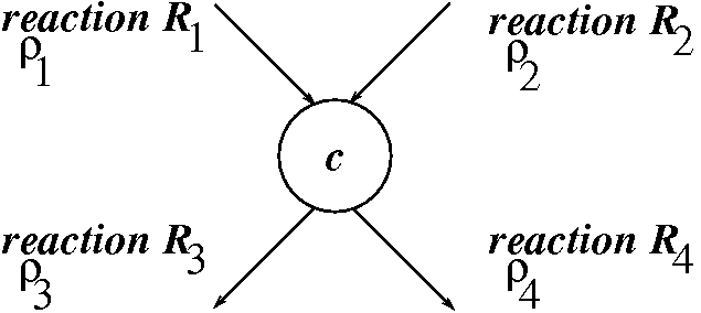
Figure 1: Complex balancing: outflows and inflows must balance at each complex $c$. The left-hand side of (14) is ${\widetilde{\kappa}}_{3}{\bar{\lambda}}^{a_{3}}+{\widetilde{\kappa}}_{4}{\bar{\lambda}}^{a_{4}}$ and the right-hand side is ${\widetilde{\kappa}}_{1}{\bar{\lambda}}^{a_{1}}+{\widetilde{\kappa}}_{2}{\bar{\lambda}}^{a_{2}}$

Foundational results in deterministic chemical network theory were obtained by Horn, Jackson, and Feinberg (see [2, 3]). One of the key theorems is that a sufficient condition for the existence of a complex balanced steady state is that the network be weakly reversible and have deficiency zero. The deficiency is computed as $n_{c}-\ell-r$, where $n_{c}$ is the number of complexes, $r$ is the rank of the matrix $\Gamma$, and $\ell$ is the number of “linkage classes” (connected components of the reaction graph). Weak reversibility means that each connected component of the reaction graph must be strongly connected. One of the most interesting features of this theorem is that no assumptions need to be made about the kinetic constants. (Of course, the choice of the vector ${\bar{\lambda}}$ will depend on kinetic constants.) We refer the reader to the citations for details on deficiency theory, as well as, of interest in the present context, several examples discussed in [10]. The theorems for weakly reversible deficiency zero networks are actually far stronger, and they show that every possible steady state of the corresponding deterministic network is complex balanced, and also that they are asymptotically stable relative to stoichiometry classes. The connection with ssCME solutions was a beautiful observation made in [1], but can be traced to the “nonlinear traffic equations” from queuing theory, described in Kelly’s textbook [5], Chapter 8 (see also [6] for a discussion),

The elements of $\Pi$ given by formula (11) add up to:

$$\sum_{k\in{\mathbb{Z}}_{\geq 0}^{n}}p_{k}\;=\;\sum_{k_{1}=0}^{\infty}\ldots\sum_{k_{n}=0}^{\infty}\,\frac{{\bar{\lambda}}_{1}^{k}}{k_{1}!}\ldots\frac{{\bar{\lambda}}_{n}^{k}}{k_{n}!}\;=\;Z:=e^{{\bar{\lambda}}_{1}}\ldots e^{{\bar{\lambda}}_{n}}$$

Thus, normalizing by the total, $\{p_{k}/Z,k\in{\mathbb{Z}}_{\geq 0}^{n}\}$ is a probability distribution. However, because of stoichiometric constraints, solutions are typically not unique, and general solutions appear as convex combinations of solutions corresponding to invariant subsets of states. A solution with only a finite number of nonzero $p_{k}$’s will then have a different normalization factor $Z$.

3.1 Conservation laws, complex-balanced case

When steady states do not form an irreducible Markov chain, the solutions of the form (11) are not the only solutions in the complex balanced case. Restrictions to each component of the Markov chain are also solutions, as are convex combinations of such restrictions. To formalize this idea, suppose that there is some subset ${\cal Z}_{0}\subseteq{\mathbb{Z}}^{n}$ with the following stoichiometric invariance property:

$$k\in{\cal Z}_{0}\;\Rightarrow\;k\pm\gamma_{j}\in{\cal Z}_{0}\quad\forall\,j=1,\ldots,m\,.$$ (15)

(The same property is then true for the complement of ${\cal Z}_{0}$.) Consider the set ${\cal Z}:={\cal Z}_{0}\bigcap{\mathbb{Z}}_{\geq 0}^{n}$. For each $k\in{\cal Z}$, the left-hand side term in equation (12) either involves an index $k-\gamma_{j}>0$, and hence also in ${\cal Z}$, or it is zero (because $k-b_{j}\geq 0$ implies $k-\gamma_{j}\geq 0$) and so it does not matter that $k-\gamma_{j}\not\in{\cal Z}$. Thus,

$$p_{k}=\left\{\begin{array}[]{ll}\displaystyle\frac{{\bar{\lambda}}^{k}}{k!}&\mbox{if }k\in{\cal Z}\\ 0&\mbox{if }k\in{\mathbb{Z}}_{\geq 0}^{n}\setminus{\cal Z}\end{array}\right.$$ (16)

is also a solution, in the complex balanced case (observe that, for indices in ${\mathbb{Z}}_{\geq 0}^{n}\setminus{\cal Z}$, equation (12) is trivially satisfied, since both sides vanish). So we need to divide by the sum $Z$ of the elements in (16) in order to normalize to a probability distribution. The restriction to ${\cal Z}$ will the unique steady state distribution provided that the restricted Markov chain has appropriate irreducibility properties.

In particular, suppose that ${\cal A}=(\alpha_{ij})\in{\mathbb{R}}^{m\times n}$ is a matrix whose nullspace includes ${\cal C}$ (for example, ${\cal A}$ could be the orthogonal complement of the “stoichiometric subspace” spanned by ${\cal C}$), and pick any vector $\beta=(\beta_{1},\ldots,\beta_{q})^{\prime}\in{\mathbb{R}}^{q}$. Then ${\cal Z}_{0}=\{k|\,{\cal A}k=\beta\}$ satisfies (15). In this case, the sum of the elements in (16) is:

$$Z(\beta_{1},\ldots,\beta_{q})=\sum_{\genfrac{}{}{0.0pt}{}{k_{1},\ldots,k_{n}\geq 0}{{\cal A}k=\beta}}\frac{\lambda_{1}^{k_{1}}}{k_{1}!}\frac{\lambda_{2}^{k_{2}}}{k_{2}!}\ldots\frac{\lambda_{n}^{k_{n}}}{k_{n}!}$$

(value is zero if the sum is empty). The normalized form of (16) has $p_{k}=0$ for $k\in{\mathbb{Z}}_{\geq 0}^{n}\setminus{\cal Z}$, and

$$p_{k}\;=\;\frac{1}{Z(\beta_{1},\ldots,\beta_{q})}\;\frac{\lambda_{1}^{k_{1}}}{k_{1}!}\frac{\lambda_{2}^{k_{2}}}{k_{2}!}\ldots\frac{\lambda_{n}^{k_{n}}}{k_{n}!}$$ (17)

for $k\in{\cal Z}$. A probabilistic interpretation of these numbers is as follows.

Suppose that we have $n$ independent Poisson random variables, $S_{i}$, $i=1,\ldots,n$, with parameters $\lambda_{i}$ respectively, so

$${\mathbb{P}}\,{\left[S_{1}=k_{1},S_{2}=k_{2},\ldots,S_{n}=k_{n}\right]}\;=\;e^{-(\lambda_{1}+\ldots+\lambda_{n})}\,\frac{\lambda_{1}^{k_{1}}}{k_{1}!}\frac{\lambda_{2}^{k_{2}}}{k_{2}!}\ldots\frac{\lambda_{n}^{k_{n}}}{k_{n}!}$$ (18)

for $k\geq 0$ (and zero otherwise). Let us introduce the following new random variables:

$$Y_{j}\,:=\;\sum_{i=1}^{n}\alpha_{ji}S_{i}\quad,\quad j=1,\ldots,q\,.$$

Observe that

$${\mathbb{P}}\,{\left[Y_{1}=\beta_{1},\ldots,Y_{m}=\beta_{q}\right]} = \sum_{\genfrac{}{}{0.0pt}{}{k_{1},\ldots,k_{n}\geq 0}{\alpha_{11}k_{1}+\ldots+\alpha_{1n}k_{n}=\beta_{1},\;\ldots,\;\alpha_{q1}k_{1}+\ldots+\alpha_{qn}k_{n}=\beta_{q}}}\;{\mathbb{P}}\,{\left[S_{1}=k_{1},S_{2}=k_{2},\ldots,S_{n}=k_{n}\right]}$$

$$= e^{-(\lambda_{1}+\ldots+\lambda_{n})}Z(\beta_{1},\ldots,\beta_{q})\,.$$

Therefore, for each $k\in{\cal Z}$, $p_{k}$ in (17) equals the following conditional probability:

$$\frac{{\mathbb{P}}\,{\left[S_{1}=k_{1},S_{2}=k_{2},\ldots,S_{n}=k_{n}\right]}}{{\mathbb{P}}\,{\left[Y_{1}=\beta_{1},\ldots,Y_{q}=\beta_{q}\right]}}\;=\;{\mathbb{P}}\,{\left[S_{1}=k_{1},S_{2}=k_{2},\ldots,S_{n}=k_{n}\,\bigl{|}\,Y_{1}=\beta_{1},\ldots,Y_{q}=\beta_{q}\right]}\,.$$

If our interest is in computing this conditional probability, the main effort goes into computing $Z(\beta_{1},\ldots,\beta_{q})$. The main contribution of the paper [10] was to provide effective algorithms for the computation of $Z(\beta_{1},\ldots,\beta_{q})$ recursively on the $\beta_{i}$’s. A package for that purpose, called MVPoisson, was included with that paper.

Conditional moments

$$E[S_{j}^{r}\,\bigl{|}\,Y_{1}=\beta_{1},\ldots,Y_{m}=\beta_{q}]\,,\;r\geq 1\,,$$

including the conditional expectation (when $r=1$), as well as centered moments such as the conditional variance, can be computed once that these conditional probabilities are known. It is convenient for that purpose to first compute the factorial moments. Recall that the $r$th factorial moment $E[W^{(r)}]$ of a random variable $W$ is defined as the expectation of $W!/(W-r)!$. For example, when $r=1$, $E[W^{(r)}]=E[W]$, and for $r=2$, $E[W^{(r)}]=E[W^{2}]-E[W]$, and thus the mean and variance of $W$ can be obtained from these. We denote the conditional factorial moment of $S_{i}$ given $Y=\beta$, as $E[S_{j}^{(r)}\,\bigl{|}\,Y]$. It is not difficult to see (Theorem 2 in [10]) that:

$$E[S_{j}^{(r)}\,\bigl{|}\,Y]\;\;=\;\;\lambda_{j}^{r}\,\cdot\,\frac{Z(\beta_{1}-r\alpha_{1j},\beta_{2}-r\alpha_{2j},\ldots,\beta_{q}-r\alpha_{qj})}{Z(\beta_{1},\ldots,\beta_{q})}$$

when all $\beta_{i}-r\alpha_{ij}\geq 0$ and zero otherwise. The paper [10] also discusses how mixed moments such as covariances can be computed.

For example, from $r=1$ we obtain a formula for the conditional mean:

$$E[S_{j}\,\bigl{|}\,Y]\;\;=\;\;\lambda_{j}\,\cdot\,\frac{Z(\beta_{1}-\alpha_{1j},\beta_{2}-\alpha_{2j},\ldots,\beta_{q}-\alpha_{qj})}{Z(\beta_{1},\ldots,\beta_{q})}$$ (19)

when all $\beta_{i}\geq\alpha_{ij}$, and zero otherwise, and from $r=2$ we obtain a formula for the conditional second moment:

$$E[S_{j}^{2}\,\bigl{|}\,Y]\;\;=\;\;\lambda_{j}^{2}\,\cdot\,\frac{Z(\beta_{1}-2\alpha_{1j},\beta_{2}-2\alpha_{2j},\ldots,\beta_{q}-2\alpha_{qj})}{Z(\beta_{1},\ldots,\beta_{q})}\;\;+\;\;E[S_{j}\,\bigl{|}\,Y]$$

when all $\beta_{i}\geq 2\alpha_{ij}$, and zero otherwise. We next work out a concrete example.

3.2 A worked example

Suppose that two molecules of species $S_{1}$ and $S_{2}$ can reversibly combine through a bimolecular reaction to produce a molecule of species $S_{3}$

$$S_{1}+S_{2}\;\xrightleftharpoons[\kappa_{2}]{\kappa_{1}}\;S_{3}\,.$$

Since the deficiency of this network is $n_{c}-\ell-r=2-1-1=0$ and it is reversible and hence weakly reversible as well, we know that there is a complex-balanced equilibrium (and every equilibrium is complex balanced). We may pick, for example, ${\bar{\lambda}}=(1,1,K)$, where $K:=\kappa_{1}/\kappa_{2}$. The count of $S_{1}$ molecules goes down by one every time that a reaction takes place, at which time the count of $S_{3}$ molecules goes up by one. Thus, the sum of the number of $S_{1}$ molecules plus the number of $S_{3}$ molecules remains constant in time, equal to their starting value, which we denote as $p$. Similarly, the sum of the number of $S_{2}$ molecules plus the number of $S_{3}$ molecules remains constant, equal to some number $n$. (In the general notations, we have $a_{11}=a_{13}=1$, $a_{22}=a_{23}=1$, $a_{12}=a_{21}=0$, $\beta_{1}=p$, $\beta_{2}=n$.) In the steady state limit as $t\rightarrow\infty$, these constraints persist. In other words, all $p_{k}$ should vanish except those corresponding to vectors $k=(k_{1},k_{2},k_{3})$ such that $k_{1}+k_{3}=p$ and $k_{2}+k_{3}=n$. The set consisting of all such vectors is invariant, so

$$p_{k}=\left\{\begin{array}[]{ll}\displaystyle\frac{{\bar{\lambda}}_{1}^{k_{1}}}{k_{1}!}\frac{{\bar{\lambda}}_{2}^{k_{2}}}{k_{2}!}\frac{{\bar{\lambda}}_{3}^{k_{3}}}{k_{3}!}&\mbox{if }k_{1}+k_{3}=p\mbox{ and }k_{2}+k_{3}=n\\ 0&\mbox{otherwise}\end{array}\right.$$

is a solution of the ssCME. In order to obtain a probability density, we must normalize by the sum $Z(p,n)$ of these $p_{k}$’s. Because of the two constraints, the sum can be expressed in terms of just one of the indices, let us say $k_{1}$. Observe that, since $k+k_{3}=p$ and $k_{3}\geq 0$, necessarily $k\leq p$. Since $k_{2}=n-k_{3}=n+k-p$ must be non-negative, we also have the constraint $k\geq\max\{0,p-n\}$. So the only nonzero terms are for $k\in\{\max\{0,p-n\},\ldots,p\}$. With $k_{3}=p-k$, $k_{2}=n-k_{3}=n+k-p$, we have:

$$Z(p,n)\;=\;\sum_{\ell=\max\{0,p-n\}}^{p}\,\frac{K^{p-\ell}}{\ell!\,(n+\ell-p)!\,(p-\ell)!}\;=\;\sum_{\ell=0}^{\min\{p,n\}}\,\frac{K^{\ell}}{(p-\ell)!\,(n-\ell)!\,\ell!}$$ (20)

The second form if the summation makes it obvious that $Z(p,n)=Z(n,p)$.

When $n\geq p$, we can also write

$$Z(p,n)\;=\;\frac{1}{n!p!}\,\sum_{\ell=0}^{p}\,\,\frac{n!}{(n-p+\ell)!}{p\choose\ell}K^{p-\ell}$$ (21)

which shows the expression as a rational function in which the numerator is a polynomial of degree $p$ on $n$. This was derived assuming that $n\geq p$, and the factorials in the denominator do not make sense otherwise. However, let us think of each term $\frac{n!}{(n-p+\ell)!}$ as the product $n(n-1)\ldots(n-p+\ell+1)$, which may include zero as well as negative numbers. With this understanding, the formula in (21) makes sense even when $n<p$. Observe that such a term vanishes for any index $\ell<p-n$. Thus, for $n<p$, (21) reduces to:

$$\frac{1}{p!}\,\sum_{\ell=p-n}^{p}\,\,\frac{1}{(n-p+\ell)!}{p\choose\ell}K^{p-\ell}$$

or equivalently, with a change of indices $~{}\ell=p-\ell$ and then using ${p\choose p-\ell}={p\choose\ell}$:

$$\frac{1}{p!}\,\sum_{\ell=0}^{n}\,\,\frac{1}{(n-\ell)!}{p\choose p-\ell}K^{\ell}\;=\;\frac{1}{p!}\,\sum_{\ell=0}^{n}\,\,\frac{1}{(n-\ell)!}{p\choose\ell}K^{\ell}\;=\;\sum_{\ell=0}^{n}\,\,\frac{K^{\ell}}{(n-\ell)!(p-\ell)!\ell!}\,.$$

In this last form, we have the same expression as the last one in (20). In conclusion, provided that we interpret the quotient of combinatorial numbers in (21) as a product that may be zero, formula (21) is valid for all $n$ and $p$, not just for $n\geq p$. In particular, we have;

$$Z(0,n)=\frac{1}{n!}\,,$$

$$Z(1,n)\;=\;\frac{Kn+1}{n!}\,,$$

$$Z(2,n)\;=\;\frac{{K}^{2}{n}^{2}+\left(-{K}^{2}+2\,K\right)n+1}{2n!}\,,$$

$$Z(3,n)\;=\;\frac{{K}^{3}{n}^{3}+\left(-3\,{K}^{3}+3\,{K}^{2}\right){n}^{2}+\left(2\,{K}^{3}-3\,{K}^{2}+3\,K\right)n+1}{3!n!}$$

and so forth. In terms of the Gauss’s hypergeometric function ₂F₀, we can also write:

$$Z(p,n)\;=\;{\frac{{\mbox{${}_{2}$F${}_{0}$}(-n,-p;\,\ ;\,K)}}{p!\,n!}}$$

The recursion on $n$ obtained by using the package MVPoisson from [10] is as follows (by symmetry, a recursion on $p$ can be found by exchanging $n$ and $p$):

$$Z(p,n+2)\;=\;{\frac{K}{n+2}}\,Z(p,n)\,+\,{\frac{-Kn+Kp-K+1}{n+2}}\,Z(p,n+1)\,.$$

Now (19) gives the conditional mean of the first species, $S_{1}$ ($j=1$ for this index, $r=1$ for the first moment, and $\lambda_{1}^{1}=1^{1}=1$) as:

$$\varphi(p,n)\,:=\;E[S_{1}\,\bigl{|}\,S_{1}+S_{3}=p,S_{2}+S_{3}=n]\;=\;\frac{Z(p-1,n)}{Z(p,n)}\,.$$

for $p\geq 1$, $n\geq 0$, and zero otherwise. For example,

$$\varphi(1,n)\;=\;\frac{1}{Kn+1}$$

$$\varphi(2,n)\;=\;\frac{2(Kn+1)}{{K}^{2}{n}^{2}+\left(-{K}^{2}+2\,K\right)n+1}\,.$$

3.3 Another worked example

Suppose that molecules of species $S_{1}$ can be randomly created and degraded, and they can also reversibly combine with molecules of $S_{2}$ through a bimolecular reaction to produce molecules of species $S_{3}$:

$$\emptyset\;\xrightarrow{\kappa_{1}}\;S_{1}\;\xrightarrow{\kappa_{2}}\;\emptyset\,,\quad S_{1}+S_{2}\;\xrightleftharpoons[\kappa_{4}]{\kappa_{3}}\;S_{3}\,.$$

There are $n_{c}=4$ complexes: $\emptyset$, $S_{1}$, $S_{1}+S_{2}$, and $S_{3}$, and $\ell=2$ linkage classes. The stoichiometry matrix

$$\Gamma\;=\;\left(\begin{array}[]{cccccccccccc}1&-1&-1&1\cr 0&0&-1&1\cr 0&0&1&-1\end{array}\right)$$

has rank $r=2$, so the deficiency of this weakly reversible network is $n_{c}-\ell-r=4-2-2=0$. Thus there is a complex-balanced equilibrium (and every equilibrium is complex balanced). We may pick, for example, ${\bar{\lambda}}=(\lambda,1,\mu)$, where $\lambda:=\frac{\kappa_{1}}{\kappa_{2}}$ and $\mu:=\frac{\kappa_{1}\kappa_{3}}{\kappa_{2}\kappa_{4}}$. Notice that there is only one nontrivial conserved quantity, $S_{2}+S_{3}=n$, since $S_{1}$ is not conserved. We have:

$$Z(n)\;=\;\sum_{\genfrac{}{}{0.0pt}{}{k_{1},k_{2},k_{3}\geq 0}{k_{2}+k_{3}=n}}\frac{\lambda_{1}^{k_{1}}}{k_{1}!}\frac{\lambda_{2}^{k_{2}}}{k_{2}!}\frac{\lambda_{3}^{k_{3}}}{k_{3}!}\;=\;\sum_{k_{1}=0}^{\infty}\frac{\lambda^{k_{1}}}{k_{1}!}\,\sum_{k_{2}=0}^{n}\frac{\mu^{n-k_{2}}}{k_{2}!(n-k_{2})!}\;=\;\frac{e^{\lambda}}{n!}(1+\mu)^{n}\,.$$

The normalized probability (16), for $k=(k_{1},k_{2},k_{3})\geq 0$ with $k_{2}+k_{3}=n$, is:

$$p_{k}\;=\;\frac{1}{Z(n)}\;\frac{\lambda^{k_{1}}}{k_{1}!}\frac{1}{k_{2}!}\frac{\mu^{k_{3}}}{k_{3}!}\;=\;\frac{n!}{e^{\lambda}(1+\mu)^{n}}\frac{\lambda^{k_{1}}\mu^{k_{3}}}{k_{1}!k_{2}!k_{3}!}$$

and as discussed earlier, this is the conditional probability

$${\mathbb{P}}\,{\left[S_{1}=k_{1},S_{2}=k_{2},S_{3}=k_{3}\,\bigl{|}\,S_{2}+S_{3}=n\right]}\,.$$

Using this expression, we may compute, for example, the conditional marginal distribution of $S_{2}$:

$${\mathbb{P}}\,{\left[S_{2}=r\,\bigl{|}\,S_{2}+S_{3}=n\right]}\;=\;\sum_{k_{1}=0}^{\infty}\frac{n!}{e^{\lambda}(1+\mu)^{n}}\frac{\lambda^{k_{1}}\mu^{(n-r)}}{k_{1}!r!(n-r)!}\;=\;{n\choose r}\,p^{r}(1-p)^{(n-r)}$$

(where we use the notation $p:=1/(1+\mu)$, so that $\mu=\frac{1-p}{p}$), which shows that this conditional marginal distribution is a binomial random variable with parameters $n$ and

$$p=\frac{\kappa_{2}\kappa_{4}}{\kappa_{2}\kappa_{4}+\kappa_{1}\kappa_{2}}\,.$$

References

• [1] D.F. Anderson, G.ย Craciun, and T.G. Kurtz. Product-form stationary distributions for deficiency zero chemical reaction networks. Bulletin of Mathematical Biology, 72(8):1947โ€“1970, 2010.
• [2] M.ย Feinberg. Chemical reaction network structure and the stability of complex isothermal reactors - I. The deficiency zero and deficiency one theorems. Chemical Engr. Sci., 42:2229โ€“2268, 1987.
• [3] M.ย Feinberg. The existence and uniqueness of steady states for a class of chemical reaction networks. Archive for Rational Mechanics and Analysis, 132:311โ€“370, 1995.
• [4] D.ย T. Gillespie. The chemical Langevin equation. Journal of Chemical Physics, 113(1):297โ€“306, 2000.
• [5] F.ย Kelly. Reversibility and Stochastic Networks. Wiley, New York, 1979.
• [6] J.ย Mairesse and H.-T. Nguyen. Deficiency zero Petri nets and product form. In G.ย Franceschinis and K.ย Wolf, editors, Applications and Theory of Petri Nets. Springer-Verlag, 2009.
• [7] S.ย P. Meyn and R.ย L. Tweedie. Stability of markovian processes iii: Foster-lyapunov criteria for continuous-time processes. Adv. Appl. Prob., 25:518โ€“548, 1993.
• [8] E.D. Sontag. Lecture notes on mathematical systems biology, Rutgers University, 2002-2015. http://www.math.rutgers.edu/~sontag/FTP_DIR/systems_biology_notes.pdf.
• [9] E.D. Sontag and A.ย Singh. Exact moment dynamics for feedforward nonlinear chemical reaction networks. IEEE Life Sciences Letters, 1:26โ€“29, 2015.
• [10] E.D. Sontag and D.ย Zeilberger. A symbolic computation approach to a problem involving multivariate Poisson distributions. Advances in Applied Mathematics, 44:359โ€“377, 2010.