The Kepler Follow-Up Observation Program. I. A Catalog of Companions to Kepler Stars from High-Resolution Imaging

Abstract

We present results from high-resolution, optical to near-IR imaging of host stars of Kepler Objects of Interest (KOIs), identified in the original Kepler field. Part of the data were obtained under the Kepler imaging follow-up observation program over seven years (2009 – 2015). Almost 90% of stars that are hosts to planet candidates or confirmed planets were observed. We combine measurements of companions to KOI host stars from different bands to create a comprehensive catalog of projected separations, position angles, and magnitude differences for all detected companion stars (some of which may not be bound). Our compilation includes 2297 companions around 1903 primary stars. From high-resolution imaging, we find that $\sim$ 10% ($\sim$ 30%) of the observed stars have at least one companion detected within 1″ (4″). The true fraction of systems with close ($\lesssim$ 4″) companions is larger than the observed one due to the limited sensitivities of the imaging data. We derive correction factors for planet radii caused by the dilution of the transit depth: assuming that planets orbit the primary stars or the brightest companion stars, the average correction factors are 1.06 and 3.09, respectively. The true effect of transit dilution lies in between these two cases and varies with each system. Applying these factors to planet radii decreases the number of KOI planets with radii smaller than 2 R_⊕ by $\sim$2-23% and thus affects planet occurrence rates. This effect will also be important for the yield of small planets from future transit missions such as TESS.

Accepted to AJ, December 6, 2016

1 Introduction

In the last few years our knowledge of extrasolar planetary systems has increased dramatically, to a large extent due to results from the Kepler mission (Borucki et al., 2010), which discovered several thousand planet candidates over its four years of operation observing more than 150,000 stars in the constellation of Cygnus-Lyra (Borucki et al., 2011a, b; Batalha et al., 2014; Burke et al., 2014; Rowe et al., 2015; Seader et al., 2015; Mullally et al., 2015; Coughlin et al., 2016). Kepler measured transit signals, which are periodic decreases in the brightness of the star as another object passes in front of it. Based on Kepler data alone, transit events are identified, then vetted, and the resulting Kepler Objects of Interest (KOIs) are categorized as planet candidates or false positives. Sorting out false positives is a complex process addressed in many publications (Fressin et al., 2013; Coughlin et al., 2014; Seader et al., 2015; Mullally et al., 2015; Desert et al., 2015; McCauliff et al., 2015; Santerne et al., 2016; Morton et al., 2016), with current estimates for false positive rates ranging from $\sim$ 10% for small planets (Fressin et al., 2013) to as high as 55% for giant planets (Santerne et al., 2016; Morton et al., 2016). It is essential to identify false positives in order to derive a reliable list of planet candidates, which can then be used to study planet occurrence rates.

Follow-up observations of KOIs play an important role in determining whether a transit signal is due to a planet or a different astrophysical phenomenon or source, such as an eclipsing binary. In addition, these observations can provide further constraints on a planet’s properties. In particular, high-resolution imaging can reveal whether a close companion was included in the photometric aperture, given that the Kepler detector has 4″ wide pixels, and photometry was typically extracted from areas a few pixels in size. The current list of Kepler planet candidates does not account for any stellar companions within $\sim$ 1″-2″of the primary, since these companions are not resolved by the Kepler Input Catalog (e.g., Mullally et al., 2015); however, if a close companion is present, an adjustment to the transit properties, mainly the transit depth and thus the planet radius, is necessary. Even if a companion is actually a background star and not bound to the planet host star, the transit depth would still be diluted by the light of the companion and thus require a correction. As shown by Ciardi et al. (2015), planet radii are underestimated by an average factor of 1.5 if all KOI host stars are incorrectly assumed to be single stars. As a result, the fraction of Earth-sized planets is overestimated, having implications on the occurrence rate of rocky and volatile-rich exoplanets (e.g., Rogers, 2015).

In the solar neighborhood, about 56% of stars are single, while the rest have one or more stellar or brown dwarf companions (Raghavan et al., 2010). High-resolution imaging of Kepler planet candidate host stars found that about one third of these stars have companions within several arcseconds (Adams et al., 2012, 2013; Dressing et al., 2014; Lillo-Box et al., 2014). Given that not all companion stars are detected, the true fraction of KOI host stars with companions is larger; Horch et al. (2014) derived that fraction to be 40%-50%, consistent with the findings of Raghavan et al. (2010).

Since the beginning of the Kepler mission in March 2009 and beyond its end in May 2013, high-resolution imaging of KOI host stars has been carried out as part of the Kepler Follow-Up Observation Program (KFOP). In addition, several observing teams that were not part of KFOP carried out imaging surveys of KOI host stars. Besides imaging, spectroscopic observations were obtained by KFOP and other teams both to constrain stellar parameters and to measure the planets’ radial velocity signals. All these observations focused on targets of the original Kepler mission and not its successor, K2. Most of the results have been posted on the Kepler Community Follow-Up Observation Program (CFOP) website, which is meant to facilitate information exchange among observers.

In this work we present in detail the follow-up observations by our KFOP team using adaptive optics in the near-infrared with instrumentation on the Keck II, Palomar 5-m, and Lick 3-m telescopes, as well as results from our optical imaging using speckle interferometry at the Gemini-North telescope, the Wisconsin-Indiana-Yale-NOAO telescope, and the Discovery Channel Telescope. We and additional, independent teams have already published other high-resolution imaging observations of KOI host stars using some of these telescopes, as well as the Calar Alto 2.2-m telescope, Multiple Mirror Telescope, Palomar 1.5-m telescope, and Hubble Space Telescope (Howell et al., 2011; Adams et al., 2012; Lillo-Box et al., 2012; Adams et al., 2013; Law et al., 2014; Dressing et al., 2014; Lillo-Box et al., 2014; Wang et al., 2014; Gilliland et al., 2015; Everett et al., 2015; Cartier et al., 2015; Wang et al., 2015a, b; Kraus et al., 2016; Baranec et al., 2016; Ziegler et al., 2016). In particular, the Robo-AO Kepler Planetary Candidate Survey observed almost all KOI host stars with planet candidates using automated laser guide star adaptive optics imaging at the Palomar 1.5-m telescope (Baranec et al., 2014; Law et al., 2014; Baranec et al., 2016; Ziegler et al., 2016).

We combine the data presented in this work with additional information on multiplicity of KOI host stars already published in the literature to create a comprehensive catalog of KOI host star multiplicity. As mentioned above and shown by Horch et al. (2014), not all companions in these “multiple” systems are bound (especially if their projected separation on the sky to the primary star is larger than about 1″); however, their presence still has to be taken into account for a correct derivation of transit depths. The high-resolution imaging observations typically resolve companions down to $\sim$ 0.1″, and we list companion stars out to 4″. We also include companions detected in the UKIRT survey of the Kepler field; the images, which are publicly available on the CFOP website, were taken in the $J$-band and typically have spatial resolutions of 0.8″-0.9″. We introduce our sample in section 2, present the imaging observations in section 3 and our main results in section 4. We discuss our results in section 5 and summarize them in section 6.

2 The Sample

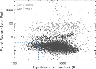
Figure 1: The planet radius versus the equilibrium temperature for the 4706 confirmed planets and planet candidates from the latest KOI cumulative table (note that some candidates with extreme values in these two parameters are not shown). The blue dashed lines delineate the region of parameter space prioritized in most of the follow-up observations ($R_{p}<$ 4 R_⊕ and $T_{eq}<$ 320 K).

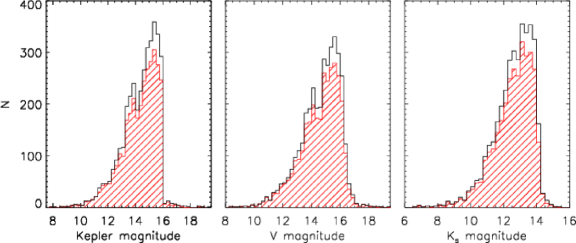
Figure 2: Histograms of the magnitudes of all KOI planet host stars (for both confirmed and candidate planets; black lines) in the Kepler bandpass (left), in the $V$-band (center), and in the 2MASS $K_{s}$ band (right). The red shaded histograms show the magnitude distributions of targets observed with high-resolution imaging.

Over the course of the Kepler mission, several KOI tables have been released, starting with the Q1-Q6 KOI table in February 2013 and ending with the Q1-Q17 DR24 table, which was delivered by the Kepler project in April 2015 and closed to further changes in September 2015. The Q1-Q6 table contained 2375 stars (with 2935 KOIs), while the latest KOI table includes 6395 stars (with 7470 KOIs). With each new KOI table, some KOIs were added, others removed, and for some the disposition (planet candidate, false positive) or planet parameters changed. The latest KOI cumulative table, which mainly incorporated objects from the latest KOI delivery (Q1-Q17 DR24), but also has KOIs from previous deliveries, contains a total of 7557 stars (with 8826 KOIs); of these, 3665 stars host at least one candidate or confirmed planet (we call these stars “planet host stars”). As of December 1, 2016, 1627 are stars with confirmed planets (2290 planets), 2244 are stars with planetary candidates (2416 possible planets), and 4014 are stars with transit events classified as false positives. Some stars have both a confirmed planet and planet candidate, or a planet (candidate) and a false positive. While the cumulative table does not represent a uniform data set, it is the most comprehensive list of KOIs with the most accurate dispositions and consistent stellar and planetary parameters.

For the Kepler Follow-Up Observation Program, targets were selected from the most recent cumulative KOI list available during each observing season. The follow-up program, as well as observing programs by other teams, focused almost entirely on planet candidates, and usually prioritized observations based on planet radii and equilibrium temperatures, giving higher priority to small ($\lesssim$ 4 R_⊕) and cool ($T_{eq}<$ 320 K) planets. A few KOI targets were selected based on interesting properties, for example stars with multiple planets. These selection criteria narrowed down the original target list of 3665 planet host stars, but even the high-priority target list contained hundreds of Kepler stars. Figure 1 shows the distribution of KOI planets (confirmed ones and candidates) among different values of equilibrium temperature and planet radius. The majority of planets (80%) have radii less than 4 R_⊕; 49% have radii less than 2 R_⊕.

Obtaining comprehensive imaging and spectroscopic data for the full KOI sample is challenging not just due to the large number of targets, but also because of the faintness of the sample: 88% of KOI planet host stars are fainter than $V$=13, and 71% are fainter than $V$=14 (see Figure 2). Many of these faint stars are hosts to Earth-sized planet candidates and are thus high-priority targets (see Everett et al. 2013 and Howell et al. 2016 for some recent results). Given the faintness of most Kepler stars, large telescopes are needed to obtain deep limits on the presence of nearby companions. In addition, high-resolution imaging with adaptive optics requires a guide star for wavefront sensing; beyond $V$ magnitudes of 14-15, the star is often too faint to be used as the guide star, and a laser guide star has to be used instead.

Different groups observed Kepler stars with high-resolution imaging techniques (adaptive optics, speckle interferometry, lucky imaging, and some space-based observations); the magnitude distributions of observed targets are shown in Figure 2 (red shaded histograms). The Robo-AO imaging at the Palomar 1.5-m telescope (Baranec et al., 2014) contributed most of the observations: of the 3665 stars that host at least one KOI planet candidate or confirmed planet, Robo-AO observed 3093. In total, 3183 planet host stars (or 87%) have high-resolution images. When considering the 4706 confirmed planets and planet candidates from the latest KOI cumulative table (the number is larger than the number of stars, since some stars have more than one planet), 90% (or 4213 planets) have been covered by high-resolution imaging. It should be noted that the imaging data are not only important for detecting companion stars, but were also useful in confirming many of the planet candidates (e.g., Batalha et al., 2011).

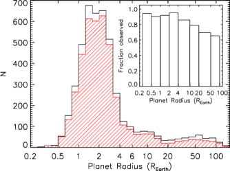
Figure 3: Histogram of planet radii of all KOI planet candidates and confirmed planets from the latest KOI cumulative table (black) and for those targeted by high-resolution imaging (red). The insert shows the fraction of planets observed for different bins of planet radii (0.25-0.5, 0.5-1, 1-2, 2-4, 4-10, 10-20, 20-50, and 50-100 R_⊕).

The distribution of planet radii (taken from the latest KOI cumulative table) for the whole sample and the high-resolution imaging sample of KOI planets can be seen in Figure 3. About 93% of planets with radii less than 4 R_⊕ were observed, while this fraction is about 76% for larger planets ($R_{p}>$ 4 R_⊕); about two thirds of KOI planets larger than 20 R_⊕ have been targeted by high-resolution imaging. This just follows from the selection criteria for targets for most of the imaging programs, since the smallest planets had the highest priority. We note that the majority of the very large planets ($R_{p}>$ 20 R_⊕) are still planet candidates (they also constitute just $\sim$ 9% of the planet sample). It is likely that most of them will not be confirmed as planets, but instead as brown dwarfs and eclipsing binaries (Santerne et al. 2016 determined a false-positive rate of 55% for giant planets with periods $<$ 400 d; Morton et al. 2016 found a mean false positive probability of 84% for planet candidates with radii $>$ 15 R_⊕). Others likely have highly inaccurate planet radii due to very uncertain stellar radii or unreliable transit fits by the Kepler pipeline (see, e.g., KOI 1298.02 and KOI 2092.03 with $R_{p}$ of 39 and 30 R_⊕, respectively, from the KOI table, which were validated as planets with radii of 1.82 R_⊕ and 4.01R_⊕, respectively; Rowe et al. 2014).

3 Observations

Table 1: High-Resolution Imaging Observations of KOI Host Stars

Telescope	Instrument	Band	PSF	N	References
(1)	(2)	(3)	(4)	(5)	(6)
Calar Alto (2.2 m)	AstraLux	$i^{\prime},z^{\prime}$	0.21″	234	Lillo-Box et al. (2012, 2014)
DCT (4 m)	DSSI	692, 880 nm	0.04″	75	this work
Gemini North (8 m)	DSSI	562, 692, 880 nm	0.02″	158	Horch et al. (2012, 2014), Everett et al. (2015), this work
HST (2.4 m)	WFC3	$F555W,F775W$	0.08″	34	Gilliland et al. (2015); Cartier et al. (2015)
Keck II (10 m)	NIRC2	$J,H,K$	0.05″	667	Wang et al. (2015a, b); Kraus et al. (2016); Baranec et al. (2016); Ziegler et al. (2016), this work
LBT (8 m)	LMIRCam	$K_{s}$	$\cdots$	24	unpublished
Lick (3 m)	IRCAL	$J,H$	0.35″	324	this work
MMT (6.5 m)	ARIES	$J,K_{s}$	0.15″	128	Adams et al. (2012, 2013); Dressing et al. (2014)
Palomar (1.5 m)	Robo-AO	$i^{\prime},LP600$	0.15″	3320	Law et al. (2014); Baranec et al. (2016); Ziegler et al. (2016)
Palomar (5 m)	PHARO	$J,H,K$	0.12″	449	Adams et al. (2012); Wang et al. (2015a, b), this work
WIYN (3.5 m)	DSSI	562, 692, 880 nm	0.05″	681	Howell et al. (2011), Horch et al. (2014), this work

Note. — Column (1) lists the telescope and the mirror size (in parentheses), column (2) the instrument used, column (3) the various bands/filters of the observations, column (4) the typical width of the point spread function in arcseconds, column (5) the number of KOI host stars observed at each facility, and column (6) the references where the data are published.

Table 2: Summary of KOI Host Stars Observed with High-Resolution Imaging Techniques

KOI	KICID	CP	PC	FP	$R_{p,min}$	KOI($R_{p,min}$)	$T_{eq,min}$	KOI($T_{eq,min}$)	$Kp$	$V$	$K_{s}$	Observatories
(1)	(2)	(3)	(4)	(5)	(6)	(7)	(8)	(9)	(10)	(11)	(12)	(13)
1	11446443	1	0	0	12.9	1.01	1344	1.01	11.34	11.46	9.85	Keck,Pal1.5,WIYN
2	10666592	1	0	0	16.4	2.01	2025	2.01	10.46	10.52	9.33	Keck,Pal1.5,WIYN
3	10748390	1	0	0	4.8	3.01	801	3.01	9.17	9.48	7.01	Keck,MMT,Pal1.5,WIYN
4	3861595	0	1	0	13.1	4.01	2035	4.01	11.43	11.59	10.19	Pal1.5,WIYN
5	8554498	0	2	0	0.7	5.02	1124	5.02	11.66	11.78	10.21	Keck,Pal1.5,Pal5,WIYN
6	3248033	0	0	1	50.7	6.01	2166	6.01	12.16	12.33	10.99	CAHA
7	11853905	1	0	0	4.1	7.01	1507	7.01	12.21	12.39	10.81	Pal1.5,Pal5,WIYN
8	5903312	0	0	1	2.0	8.01	1752	8.01	12.45	12.62	11.04	Pal5
10	6922244	1	0	0	14.8	10.01	1521	10.01	13.56	13.71	12.29	Pal1.5,Pal5,WIYN
11	11913073	0	0	1	10.5	11.01	1031	11.01	13.50	13.75	11.78	Pal5
12	5812701	1	0	0	14.6	12.01	942	12.01	11.35	11.39	10.23	CAHA,Keck,Lick,Pal1.5,WIYN
13	9941662	1	0	0	25.8	13.01	3560	13.01	9.96	9.87	9.43	DCT,Gem,Keck,MMT,Pal1.5,Pal5,WIYN
14	7684873	0	0	1	5.9	14.01	2405	14.01	10.47	10.62	9.84	Pal5
17	10874614	1	0	0	13.4	17.01	1355	17.01	13.30	13.41	11.63	Pal1.5,Pal5
18	8191672	1	0	0	15.3	18.01	1640	18.01	13.37	13.47	11.77	Gem,Pal1.5,Pal5
20	11804465	1	0	0	18.2	20.01	1338	20.01	13.44	13.58	12.07	Pal1.5,Pal5,WIYN
22	9631995	1	0	0	12.2	22.01	1000	22.01	13.44	13.64	12.04	Pal1.5,Pal5,WIYN
28	4247791	0	0	1	83.1	28.01	1412	28.01	11.26	11.79	10.29	Pal5,WIYN
31	6956014	0	0	1	45.3	31.01	6642	31.01	10.80	11.92	7.94	Pal5
33	5725087	0	0	1	63.1	33.01	9970	33.01	11.06	11.10	7.59	Pal5
41	6521045	3	0	0	1.3	41.02	674	41.03	11.20	11.36	9.77	CAHA,Keck,MMT,Pal1.5,Pal5,WIYN
42	8866102	1	0	0	2.5	42.01	859	42.01	9.36	9.60	8.14	Keck,MMT,Pal1.5,Pal5,WIYN
44	8845026	0	0	1	11.9	44.01	462	44.01	13.48	13.71	11.66	Keck,Lick,Pal1.5,WIYN
46	10905239	2	0	0	0.9	46.02	1075	46.02	13.77	13.80	12.01	Keck,Pal1.5,WIYN
49	9527334	1	0	0	2.7	49.01	886	49.01	13.70	13.56	11.92	CAHA,Pal1.5,WIYN
51	6056992	0	1	0	49.8	51.01	833	51.01	13.76	14.02	14.31	CAHA,Pal1.5,WIYN

Note. — The full table is available in a machine-readable form in the online journal. A portion is shown here for guidance regarding content and form.

Column (1) lists the KOI number of the star, column (2) its identifier from the Kepler Input Catalog (KIC), columns (3) to (5) the number of confirmed planets (CP), planet candidates (PC), and false positives (FP), respectively, in the system, column (6) radius of the smallest planet in the system (in R_⊕) and column (7) its KOI number, column (8) the equilibrium temperature of the coolest planet in the system (in K) and column (9) its KOI number, columns (10) to (12) the Kepler, $V$, and $K_{s}$ magnitudes of the KOI host stars, and column (13) the observatories where data were taken. Note that if a system contains both planets and false positives, only the planets are used to determine the smallest planet radius and lowest equilibrium temperature. The abbreviations in column (13) have the following meaning: CAHA – Calar Alto, DCT – Discovery Channel Telescope, Gem – Gemini N, HST – Hubble Space Telescope, Keck – Keck II, LBT - Large Binocular Telescope, Lick – Lick-3m, MMT – Multiple Mirror Telescope, Pal1.5 – Palomar-1.5m, Pal5 – Palomar-5m, WIYN – Wisconsin-Indiana-Yale-NOAO telescope.

Table 3: Summary of High-Resolution Imaging Observations of KOI Host Stars

KOI	KICID	Telescope	Instrument	Filter/Band	PSF (″)	$\Delta m$	$d_{\Delta m}$ (″)	Obs. Date
(1)	(2)	(3)	(4)	(5)	(6)	(7)	(8)	(9)
1	11446443	Keck	NIRC2	$K^{\prime}$	$\cdots$	7.60	0.50	2012-07-06
1	11446443	Keck	NIRC2	$K^{\prime}$	$\cdots$	4.11	0.03	2012-07-06
1	11446443	Keck	NIRC2	$K^{\prime}$	$\cdots$	5.90	0.50	2012-07-06
1	11446443	Keck	NIRC2	$J$	0.04	5.61	0.5	2014-07-17
1	11446443	Keck	NIRC2	$H$	0.04	6.07	0.5	2014-07-17
1	11446443	Keck	NIRC2	$Ks$	0.04	4.93	0.5	2014-07-17
1	11446443	Pal1.5	Robo-AO	$i^{\prime}$	0.12	5.40	0.5	2012-07-16
1	11446443	WIYN	DSSI	880 nm	0.05	2.73	0.2	2011-06-13
1	11446443	WIYN	DSSI	692 nm	0.05	3.28	0.2	2011-06-13
1	11446443	WIYN	DSSI	880 nm	0.05	2.67	0.2	2013-09-21
1	11446443	WIYN	DSSI	692 nm	0.05	3.50	0.2	2013-09-21
1	11446443	WIYN	DSSI	880 nm	0.05	2.84	0.2	2013-09-23
1	11446443	WIYN	DSSI	692 nm	0.05	2.82	0.2	2013-09-23
2	10666592	Keck	NIRC2	$K^{\prime}$	$\cdots$	7.20	0.50	2012-08-14
2	10666592	Keck	NIRC2	$K^{\prime}$	$\cdots$	5.80	0.50	2012-08-14
2	10666592	Keck	NIRC2	$K^{\prime}$	$\cdots$	4.56	0.03	2014-08-13
2	10666592	Pal1.5	Robo-AO	$i^{\prime}$	0.12	4.60	0.2	2012-07-16
2	10666592	WIYN	DSSI	880 nm	0.05	2.78	0.2	2011-06-13
2	10666592	WIYN	DSSI	692 nm	0.05	4.01	0.2	2011-06-13
3	10748390	Keck	NIRC2	$K^{\prime}$	$\cdots$	7.70	0.50	2012-07-05
3	10748390	Keck	NIRC2	$K^{\prime}$	$\cdots$	4.17	0.03	2012-07-05
3	10748390	MMT	ARIES	$Ks$	0.15	8.00	1.0	2012-10-02
3	10748390	MMT	ARIES	$J$	0.20	8.00	1.0	2012-10-02
3	10748390	Pal1.5	Robo-AO	$i^{\prime}$	0.12	4.60	0.2	2012-07-16
3	10748390	WIYN	DSSI	880 nm	0.05	3.45	0.2	2011-06-13
3	10748390	WIYN	DSSI	692 nm	0.05	3.76	0.2	2011-06-13
4	3861595	Pal1.5	Robo-AO	$i^{\prime}$	0.12	$\cdots$	$\cdots$	2012-07-16
4	3861595	WIYN	DSSI	692 nm	0.05	3.06	0.2	2010-09-17
4	3861595	WIYN	DSSI	562 nm	0.05	3.46	0.2	2010-09-17
4	3861595	WIYN	DSSI	692 nm	0.05	3.58	0.2	2010-09-18
4	3861595	WIYN	DSSI	562 nm	0.05	4.01	0.2	2010-09-18
5	8554498	Keck	NIRC2	$K^{\prime}$	$\cdots$	6.70	0.50	2012-08-14
5	8554498	Keck	NIRC2	$K^{\prime}$	$\cdots$	1.12	0.03	2012-08-14
5	8554498	Keck	NIRC2	$K^{\prime}$	0.05	8.00	0.5	2013-08-20
5	8554498	Pal1.5	Robo-AO	$i^{\prime}$	0.12	4.60	0.2	2012-07-16
5	8554498	Pal5	PHARO	$J$	0.24	5.08	0.5	2009-09-10
5	8554498	WIYN	DSSI	692 nm	0.05	3.02	0.2	2010-09-17
5	8554498	WIYN	DSSI	562 nm	0.05	3.44	0.2	2010-09-17
5	8554498	WIYN	DSSI	692 nm	0.05	3.13	0.2	2010-09-18
5	8554498	WIYN	DSSI	562 nm	0.05	3.50	0.2	2010-09-18
5	8554498	WIYN	DSSI	692 nm	0.05	3.12	0.2	2010-09-21
5	8554498	WIYN	DSSI	880 nm	0.05	2.38	0.2	2010-09-21
6	3248033	CAHA	AstraLux	$i^{\prime}$	0.16	3.24	0.5	2013-06-23

Note. — The full table is available in a machine-readable form in the online journal. A portion is shown here for guidance regarding content and form.

Column (1) lists the KOI number of the star, column (2) its identifier from the Kepler Input Catalog (KIC), column (3) the telescope where the images were taken (see the notes of Table 2 for an explanation of the abbreviations), column (4) the instrument used, column (5) the filter/band of the observation, column (6) the typical width of the stellar PSF in arcseconds, column (7) the typical sensitivity $\Delta m$ (usually 5$\sigma$) at a certain separation (in arcseconds) from the primary star, column (8) the separation for the $\Delta m$ value from column (7), and column (9) the date of the observation (in year-month-day format). Sensitivity curves with $\Delta m$ values measured at a range of separations are available on the CFOP website at https://exofop.ipac.caltech.edu/cfop.php.

Several observing facilities were used to obtain high-resolution images of KOI host stars. Table 1 lists the various telescopes, instruments used, filter bandpasses, typical PSF widths, number of targets observed, and main references for the published results. The four main observing techniques employed are adaptive optics (Keck, Palomar, Lick, MMT), speckle interferometry (Gemini North, WIYN, DCT), lucky imaging (Calar Alto), and imaging from space with HST. A total of 3557 KOI host stars were observed at 11 facilities with 9 different instruments, using filters from the optical to the near-infrared. In addition, 10 of these stars were also observed at the 8-m Gemini North telescope by Ziegler et al. (2016) using laser-guide-star adaptive optics. The largest number of KOI host stars (3320) were observed using Robo-AO at the Palomar 1.5-m telescope (Baranec et al., 2014; Law et al., 2014; Baranec et al., 2016; Ziegler et al., 2016).

Table 2 lists the KOI host stars that were observed with high-resolution imaging, together with the observatories that were used and some of the planet parameters and stellar magnitudes. Some KOIs that are currently dispositioned as false positives (i.e., there is no planet, candidate or confirmed, orbiting the star) were observed, too, since at the time their observations were carried out the disposition was either set to planet candidate or was not set. Of the 3557 observed stars, almost two thirds (61% or 2187 stars) were observed at only one telescope facility with one instrument, usually just using one filter; 696 stars were observed at two telescopes, while the remaining 674 stars were observed at two or more facilities. Combining the data from all telescopes, 1431 stars were observed with two or more filters.

In Table 3 we provide a more detailed summary of the high-resolution observations, including the dates of the observations, the telescopes, instruments, and filters used, and, for most observations, the typical PSF width and sensitivity (given as $\Delta m$ – typically a 5$\sigma$ measurement – at a certain separation from the primary star). A total of 8332 observations were carried out from 2009 September to 2015 October covering 3557 stars. The median and mean PSF widths of all the high-resolution imaging observations where this parameter was reported are both 0.12″; $\sim$ 90% of the observations have PSF widths smaller than 0.16″. For the image sensitivities, the majority of $\Delta m$ values are given at a projected separation of 0.5″ (for most AO observations and lucky imaging) or 0.2″ (for speckle observations) from the primary star. Median values for $\Delta m$ at 0.2″ and 0.5″ are 3.0 and 6.0, respectively. The $\Delta m$ values at 0.03″ from the primary star are measurements from images using non-redundant aperture masking at the Keck telescope (Kraus et al., 2016); this technique enables binaries to be resolved at projected separations of just a few tenths of an arcsecond (see Kraus et al., 2016). The median $\Delta m$ value at 0.03″ is 3.94.

For this work, we reduced and analyzed our (for the most part not yet published) AO observations at Keck, Palomar, and Lick (see section 3.1), and our speckle imaging observations from Gemini North, WIYN, and DCT (see section 3.2). We also gathered results from all Kepler follow-up imaging observations, carried out by KFOP and other observing teams, from the literature and a few unpublished results from CFOP. These observations will be briefly introduced in section 3.3.

3.1 Adaptive Optics at Keck, Palomar, and Lick

Table 4: Observing Log for our Adaptive Optics Runs at Keck, Palomar, and Lick

Telescope and Instrument	UT Dates (YYYYMMDD)
KeckII, NIRC2	20120505, 20120606, 20120704, 20120825, 20130615, 20130706, 20130723,
	20130808, 20130819, 20140612, 20140613, 20140702, 20140717, 20140718,
	20140811, 20140812, 20140817, 20140904, 20140905, 20150714, 20150731,
	20150804, 20150806, 20150807
Palomar Hale, PHARO	20090907, 20090908, 20090909, 20090910, 20100630, 20100701, 20100702,
	20120907, 20120908, 20130624, 20140710, 20140711, 20140712, 20140713,
	20140714, 20140716, 20140717, 20140807, 20140808, 20140810, 20140813,
	20150527, 20150528, 20150529, 20150827, 20150828, 20150829, 20150830,
	20150831
Lick Shane, IRCAL	20110908, 20110909, 20110910, 20110911, 20110912, 20120706, 20120707,
	20120708, 20120709, 20120710, 20120805, 20120806, 20120901, 20120902,
	20120903, 20130715, 20130716, 20130717, 20130718, 20130916, 20130918

We carried out observations at the Keck, Palomar, and Lick Observatory using the facility adaptive optics systems and near-infrared cameras from 2009 to 2015. Table 4 lists the various observing runs whose results are presented here. At Palomar and Lick, we used the targets themselves as natural guide stars (NGS) for the adaptive optics system, while at Keck we used our targets as natural guide stars when they were sufficiently bright, and the laser guide star (LGS) for the fainter targets (roughly $Kp$ $>$ 14.5). The majority of our nights at Keck employed NGS.

At Keck, we observed with the 10-m Keck II telescope and NIRC2 (Wizinowich et al., 2004). The pixel scale of NIRC2 was 0.01″/pixel, resulting in a field of view of about 10″$\times$ 10″. We observed our targets in a narrow $K$-band filter, Br$\gamma$, which has a central wavelength of 2.1686 $\mu$m. In most cases, when a companion was detected, we also observed the target in a narrow-band $J$ filter, $Jcont$, which is centered at 1.2132 $\mu$m. We dithered the target in a 3-point pattern to place it in all quadrants of the array except for the lower left one (which has somewhat larger noise levels).

At Palomar, we used the 5-m Hale telescope with PHARO (Hayward et al., 2001). We used the 0.025″/pixel scale, which yielded a field of view of about 25″$\times$ 25″. As at Keck, we typically used a narrow-band filter in the $K$-band, Br$\gamma$ centered at 2.18 $\mu$m, to observe our targets. When a companion was detected, we usually also observed our targets in the $J$ filter (centered at 1.246 $\mu$m). We dithered each target in a 5-point quincunx pattern to place it in all four quadrants of the array and at the center.

At Lick, we used the 3-m Shane telescope and IRCAL (Lloyd et al., 2000). With its 0.075″/pixel scale, it offered a field of view of about 19″$\times$ 19″. We observed our targets with the $J$ filter (centered at 1.238 $\mu$m) or the $H$ filter (centered at 1.656 $\mu$m). Each target was dithered on the array in a 5-point pattern.

At all three telescopes, the integration time for each target varied, depending on its brightness. It was typically between 5 and 60 sec per frame, for a total exposure time of 10-15 minutes. Some of the fainter targets required longer exposures, but, in order to cover a reasonable number of targets on any given night, we tried to limit the time spent on any target to about half an hour. Over all observing runs at Keck, Palomar, and Lick, we observed 253, 317, and 310 unique KOI host stars, respectively. Some were observed in more than one filter, and some were observed at more than one telescope. Overall, we covered 770 unique KOI host stars with our adaptive optics imaging.

To reduce the images, we first created nightly flatfields, and for each target we constructed a sky image by median-filtering and coadding the dithered frames. Each frame was then flatfielded and sky-subtracted, and the dithered frames combined. The final, co-added images obtained at Palomar are typically 14″$\times$ 14″ in size, but there is a spread ranging from 10″ to 34″. The final images from Keck are usually 4″$\times$ 4″ in size, with some up to 16″$\times$ 16″. Finally, the reduced Lick images are $\sim$ 23″$\times$ 23″ in size.

We used aperture photometry to measure the relative brightness of the stars in each reduced frame. We used an aperture radius equal to the FWHM of the primary star and a sky annulus between about 3 and 5 times the FWHM. For close companions, we reduced the FWHM to minimize contamination, and we adjusted the sky annulus to exclude emission from the sources. The FWHM values varied depending on the observing conditions; at Palomar, the mean and median FWHM values were 6.6 and 5.4 pixels (or 0.165″ and 0.135″), respectively, at Keck 5.7 and 5.3 pixels (0.057″ and 0.053″), and at Lick 5.0 and 4.6 pixels (0.375″ and 0.345″). The $J$-, $H$-, and $K$-band measurements were converted from data numbers to magnitudes using the magnitudes of the primary source from the Two Micron All Sky Survey (2MASS; Skrutskie et al., 2006).

We also measured image sensitivities for each target by calculating the standard deviation of the background ($\sigma$) in concentric annuli around the main star; the radii of the annuli were set to multiples of the FWHM of the primary star. As can be seen from Table 1, the typical FWHM of the stellar PSF was 0.05″ at Keck, 0.12″ at Palomar, and 0.2″ at Lick. Within each ring, we determined 5$\sigma$ limits.

Some of the AO data presented here (mostly from Palomar and Keck) have already been published in the literature (Torres et al., 2011; Batalha et al., 2011; Fortney et al., 2011; Ballard et al., 2011, 2013; Borucki et al., 2012, 2013; Gautier et al., 2012; Adams et al., 2012; Marcy et al., 2014; Everett et al., 2015; Torres et al., 2015; Teske et al., 2015); they were typically used to confirm Kepler planet candidates.

3.2 Speckle Interferometry

Table 5: Observing Log for our Speckle Interferometry Runs at WIYN, Gemini North, and DCT

Telescope	UT Dates (YYYYMMDD)
WIYN	20100618, 20100619, 20100620, 20100621, 20100622, 20100624, 20100917,
	20100918, 20100919, 20100920, 20100921, 20101023, 20101024, 20101025,
	20110611, 20110612, 20110613, 20110614, 20110615, 20110616, 20110907,
	20110908, 20110909, 20110910, 20110911, 20120927, 20120929, 20120930,
	20121001, 20121003, 20121004, 20121005, 20130525, 20130526, 20130527,
	20130528, 20130921, 20130922, 20130923, 20130924, 20130925, 20150927,
	20150928, 20150929, 20150930, 20151002, 20151003, 20151004, 20151023,
	20151024, 20151027
Gemini North	20120727, 20120728, 20130725, 20130726, 20130727, 20130728, 20130729,
	20130731, 20140719, 20140722, 20140723, 20140724, 20140725, 20150711,
	20150712, 20150714, 20150715, 20150718, 20150719, 20150720
DCT	20140321, 20140323, 20140617, 20140618, 20141001, 20141002

Our team also carried out speckle imaging using the Differential Speckle Survey Instrument (DSSI; Horch et al. 2009, 2010) at Gemini North, the Wisconsin-Indiana-Yale-NOAO (WIYN) telescope, and at the Discovery Channel Telescope (DCT) from 2010 to 2015. Table 5 lists the various observing dates at the three telescopes. At the 8-m Gemini North telescope, 158 unique KOI host stars were observed, while at the 3.5-m WIYN telescope, 681 stars were targeted. The more recent observing runs at the 4-m DCT telescope covered 75 stars. Overall, at all three telescopes the observations were directed at 828 unique KOI host stars.

Targets were observed simultaneously in two bands, centered at 562 nm and 692 nm (both with a band width of 40 nm), or at 692 nm and 880 nm (the latter with a band width of 50 nm). Some targets have data in all three bands. The field of view of the speckle images is smaller than that of the AO images, about 3″ on each side, but the PSF widths are narrower (0.02″-0.05″), resulting in better spatial resolution. Some of the results on DSSI observations of KOIs can be found in Howell et al. (2011), Horch et al. (2012, 2014), Everett et al. (2015), and Teske et al. (2015).

A description of typical observing sequences done for KOI host stars using DSSI and a detailed explanation of the data reduction methods can be found in Horch et al. (2011) and Howell et al. (2011). In addition, M. E. Everett et al. (2017, in preparation) will document all of the speckle imaging in more detail. Here we briefly outline the reduction and analysis of the speckle data. The reduction of speckle observations takes place in both image and Fourier space. First, the autocorrelation function and triple correlation function are calculated for each frame of an image set centered on the target star’s speckle pattern. These functions are averaged over all frames and then converted through Fourier transforms into a power spectrum and bispectrum. The same procedure is applied to the speckle observations of single (point source) calibrator stars. For each target, the power spectrum is divided by the power spectrum of the point source calibrator to yield a fringe pattern, which contains information on the separation, relative position angle, and brightness of any pair of stars, or a pattern containing no significant fringes in the case of a single star. Using the methods described by Meng et al. (1990), a reconstructed image of the target star and its surroundings is made from the power spectrum and bispectrum (the bispectrum contains the phase information to properly orient the position angle).

We fit a model fringe pattern to the observations to determine the separation and position angle of any detected companion relative to the primary, as well as the magnitude difference between companion and primary encoded in the amplitude of the fringes. Besides the relative positions and magnitudes, we also derived background sensitivities in the speckle fields using the reconstructed images. We used the fluxes relative to the primary star of all local maxima and minima noise features in the background of the reconstructed image to derive average $\Delta m$ values and their standard deviation within certain bins of separation from the primary star. From this, we adopted a contrast curve 5$\sigma$ brighter than the average $\Delta m$ values to represent the detection limits for any given image.

Given this reduction and analysis method, it is difficult to determine individual uncertainties for the $\Delta m$ measurements of detected companions (the most challenging of the measurements we made). We took a conservative approach and adopted an uncertainty of 0.15 mag for all measurements (roughly twice the uncertainty determined empirically in, e.g., Horch et al. 2011, as KOI host stars are almost all fainter stars). When comparing targets observed in the same band multiple times, we note just a few outliers that are likely affected by poor fits between the model and observed power spectrum, or a poor match between the science target and point source calibrator. In addition, the photometric accuracy of speckle observations degrades with a combination of poor seeing and large angular separations, as well as with fainter targets.

3.3 Other High-Resolution Imaging

Wang et al. (2015a, b) used the adaptive optics systems at Keck and Palomar with NIRC2 and PHARO, respectively, and typically observed each target with the $J$-, $H$-, and $K$-band filters.

Adams et al. (2012, 2013) and Dressing et al. (2014) mainly used the $K_{s}$ filter in their AO observations at the MMT; in addition, they often used the $J$-band filter when a companion was detected in the $K_{s}$ image. The field of view of the ARIES instrument on the MMT was 20″$\times$ 20″, somewhat smaller than that of PHARO at Palomar, and the FWHM of the stellar images varied between about 0.1″ and 0.6″.

Kraus et al. (2016) employed adaptive optics imaging and also nonredundant aperture-mask interferometry at Keck with the NIRC2 instrument; the latter technique is limited only by the diffraction limit of the 10-m Keck telescope. They used the $K^{\prime}$ filter for their observations.

Baranec et al. (2016) and Ziegler et al. (2016) observed a sample of KOI host stars at Keck using mostly the $K^{\prime}$ filter on NIRC2. With the Robo-AO imaging at the Palomar 1.5-m telescope, Law et al. (2014), Baranec et al. (2016), and Ziegler et al. (2016) covered a total of 3320 KOI host stars. For most observations, they used a long-pass filter whose window starts at 600 nm ($LP600$), which is similar to the Kepler bandpass; they also took data for some stars in the Sloan $i$-band filter and, more rarely, Sloan $r$ and $z$ filters. Typical FWHM of the observed stellar PSF amounted to 0.12″-0.15″; the images covered a field of view of 44″ $\times$ 44″.

Lillo-Box et al. (2012, 2014) used the 2.2-m Calar Alto telescope with the AstraLux instrument to obtain diffraction-limited imaging with the lucky imaging technique, typically observing in the $i$- and $z$-band filters. This technique involves taking a very large number of short exposures and then combining only those images with the best quality (i.e., with the highest Strehl ratios). The FWHM of the stellar PSF in their 24″ $\times$ 24″ images was typically 0.21″, which is somewhat larger than the value from AO images ($\sim$ 0.15″).

HST imaging using the WFC3 was carried out in the $F555W$ and $F775W$ bands (Gilliland et al., 2015; Cartier et al., 2015). The images spanned a relatively large field of view of 40″$\times$ 40″, and the typical FWHM of the stellar PSF was 0.08″.

One additional facility, the 8-m Large Binocular Telescope, was used with LMIRCam to observe 24 KOI host stars in the $K_{s}$ band, but results have not yet been published and are not available on CFOP. Except for one of these 24 stars (which has only one false positive transit signal), all have been observed with one or more other facilities, too.

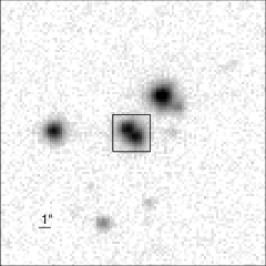
Figure 4: Images of KOI 2174 in the $J$-band filter. The target star is at the center of the images, and north is up and east is to the left. Left: 2MASS, with an image scale of 1″/pixel. The box shows the size of the UKIRT image displayed on the right. Right: UKIRT, with an image scale of 0.2″/pixel. The box shows the size of the Keck images shown in Figure 5.

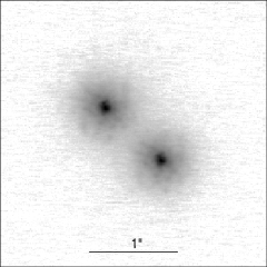
Figure 5: Images of KOI 2174 observed with Keck/NIRC2 in the $J$-band filter (left) and in the $K$-band filter (right). The image scale is 0.01″/pixel; the images shown are 3″ on each side. North is up and east is to the left.

3.4 Other Imaging

3.4.1 UKIRT Survey

The Kepler field was observed at the United Kingdom Infrared Telescope (UKIRT) in 2010 using the UKIRT Wide Field Camera (WFCAM). The images were taken in the $J$-band and have a typical spatial resolution of 0.8″-0.9″. For each KOI host star, UKIRT image cut-outs and tables with nearby stars are available on CFOP. We used that information to extract companions located within a radius of 4″ around each KOI host star. We considered all sources listed in the UKIRT catalog that were not affected by saturation; thus, we also included objects with a high “galaxy probability” ($>0.9$), which applies to most faint sources, as well as objects with a larger “noise probability” ($>0.1$). We vetted each companion by checking the UKIRT images for artifacts or spurious source detections. This vetting process led us to identify the following 18 KOIs as galaxies (which are clearly resolved in the UKIRT images): 51, 311, 1836, 1926, 2826, 3172, 3174, 3193, 3206, 5014, 5190, 5238, 5595, 5668, 6817, 6864, 7213, 7612. Most are identified as false positives, but KOI 51, 3193, and 3206 are dispositioned as planet candidates.

We cross-checked the UKIRT detections with 2MASS, which has a much lower spatial resolution (1″/pixel for 2MASS, compared to 0.2″/pixel for UKIRT). We found that only companions at separations $\gtrsim$ 3.5″ are resolved by 2MASS, and only if the companion is not too faint ($\Delta m\lesssim 4$) and the region within 4″-5″ from the star is not crowded by multiple sources. The search for companions in 2MASS data yielded $H$- and $K_{s}$-band magnitudes for some of the wider companions.

To illustrate the importance of high-resolution imaging, Figures 4 and 5 show $J$-band images of KOI 2174 (which is a star with 3 planetary candidates with $R_{p}<$ 2 R_⊕) with increasing spatial resolution. The 2MASS images do not resolve the central $\sim$ 0.9″ binary; even though it is discernible in the UKIRT image, the UKIRT source catalog does not resolve the two sources (Fig. 4). The only companion within 4″ resolved by the UKIRT (and also 2MASS) catalog is the star at a separation of 3.8″ and position angle of $\sim$ 320° (i.e., to the northwest). The small field of view of Keck (Fig. 5) does not include any star beyond about 2.5″ from the close binary, but the Keck images clearly separate the two components of the 0.9″ binary.

3.4.2 UBV Survey

Everett et al. (2012) carried out a survey of the Kepler field in 2011 using the NOAO Mosaic-1.1 Wide Field Imager on the WIYN 0.9-m telescope. They observed the field in $UBV$ filters; the FWHM of the stellar PSF due to seeing ranged from 1.2″ to 2.5″ in the $V$-band (with somewhat larger values in the $U$- and $B$-band). The source catalog and the images are available on CFOP. We searched the catalog to find companions within 4″ for each KOI host star. Due to the lower spatial resolution, just 132 KOI host stars were found to have such a companion; the smallest companion separation is 1.4″. Almost all the companions detected in the $UBV$ survey are also found in UKIRT images. In a few cases their positions disagree somewhat (up to $\sim$ 0.5″ in radial separation and 10°-15° in position angle relative to the primary star) due to the presence of additional nearby stars, which make the positions from the lower-resolution $UBV$ data more uncertain. In one case (KOI 6256), there are two companion stars detected in the $UBV$ survey, but only one of them is also resolved in the UKIRT $J$-band image. In another case (KOI 5928), a companion is detected at a projected separation of 3.3″ in $UBV$ images, but the primary star is saturated in the UKIRT data, and so no reliable position and magnitude for the companion could be determined in the $J$-band.

4 Results

4.1 Companions and Sensitivity Curves

4.1.1 Keck, Palomar, and Lick

Figure 6: Image sensitivities for observations of Kepler stars with the Keck 10-m telescope. The median sensitivities and quartiles are plotted with black symbols. The median FWHM of the stellar images was 0.05″.

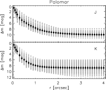
Figure 7: Image sensitivities for observations of Kepler stars with the Palomar 5-m telescope. The median sensitivities and quartiles are plotted with black symbols. The median FWHM of the stellar images was 0.13″ for the $J$-band and 0.12″ for the $K$-band.

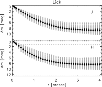
Figure 8: Image sensitivities for observations of Kepler stars with the Lick 3-m telescope. The median sensitivities and quartiles are plotted with black symbols. The median FWHM of the stellar images was 0.43″ for the $J$-band and 0.31″ for the $H$-band.

Table 6: Typical FWHM values of the stellar PSFs for the AO and speckle images

Telescope	Technique	Band	Mean FWHM	Median FWHM
Keck	AO	$J$	0.063″	0.053″
		$K$	0.057″	0.053″
Palomar	AO	$J$	0.166″	0.127″
		$K$	0.140″	0.120″
Lick	AO	$J$	0.453″	0.431″
		$H$	0.347″	0.314″
Gemini North	speckle	562, 692, 880 nm	0.02″	0.02″
WIYN	speckle	562, 692, 880 nm	0.05″	0.05″
DCT	speckle	692, 880 nm	0.04″	0.04″

As described in section 3.1, we have observed several hundred KOI host stars at Keck, Palomar, and Lick. Here we present the results of our measurements of the image sensitivity and of companions detected in the images. For the former, we combined the measurements from each image (5$\sigma$ limits in annuli around the main star) to determine the median, lower and upper quartiles for each filter at each telescope; the resulting plots are shown in Figures 6 to 8. Typical FWHM values (mean and median) of the stellar PSFs are listed in Table 6; we used the 5$\sigma$ limits measured at radial separations equal to multiples of the FWHM and interpolated them at the radial values shown in the plots. Of the three observing facilities, we reach the highest sensitivity close to the primary star with Keck; already at a separation of $\sim$ 0.5″ we reach a median sensitivity of $\Delta m\sim$ 8 mag in the $K$-band. At Palomar, the median sensitivity reaches $\Delta m\sim$ 8 mag in the $K$-band at $\sim$ 1″ from the primary. We are particularly sensitive to companions in the $J$-band; in this band, at a separation of a few arcseconds, we are sensitive to companions up to 10 magnitudes fainter than the primary. Finally, at Lick we achieve a median sensitivity of $\Delta m\sim$ 8 mag in both the $J$- and $H$-band at about 2.5″ from the primary.

For those KOI host stars where a companion was detected, we measured the position and brightness of that companion relative to the primary. Figures 9 to 11 show the companions detected within 4″ in our Keck, Palomar, and Lick images; for each telescope, detections in two filter bands are shown ($J$ and $K$ for Keck and Palomar, $J$ and $H$ for Lick). Some companions have measurements in both filters. Of the 253 unique KOI stars observed at Keck, 75 have at least one companion detected within 4″; for the 317 KOI stars observed at Palomar, this number is 116, and for the 310 KOI stars observed at Lick, 71 have such companions (see Table 7). In Table 7, we also list the number of KOI stars with one, two, three, and even four companions. These are just the companions we detected; there could be more companions that were too faint or too close to the primary stars to be found in our data. Overall, at all three telescopes 770 unique KOI host stars were observed, and 242 of these stars have companions detected within 4″; thus, in our AO sample the observed fraction of systems consisting of at least two stars within 4″ is 31% ($\pm$2%, assuming Poisson statistics).

Figure 9: Magnitude difference versus radial separation for all companions detected around Kepler stars with the Keck 10-m telescope in the $J$-band (top) and $K$-band (bottom). The dashed lines are the median image sensitivities from Figure 6.

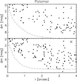
Figure 10: Magnitude difference versus radial separation for all companions detected around Kepler stars with the Palomar 5-m telescope in the $J$-band (top) and $K$-band (bottom). The dashed lines are the median image sensitivities from Figure 7.

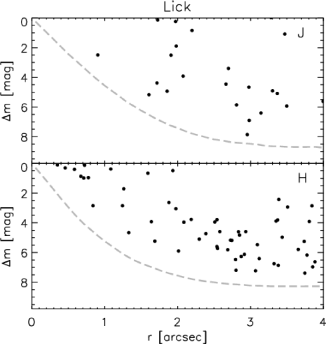
Figure 11: Magnitude difference versus radial separation for all companions detected around Kepler stars with the Lick 3-m telescope in the $J$-band (top) and $H$-band (bottom). The dashed lines are the median image sensitivities from Figure 8.

Table 7: Number of KOI stars with Detected Companions and Fraction of Multiple Systems in AO and Speckle Images

Telescope	N	Ncomp	Ncomp=1	Ncomp=2	Ncomp=3	Ncomp=4	f($<$1″)	f($<$4″)
(1)	(2)	(3)	(4)	(5)	(6)	(7)	(8)	(9)
Keck	253	75	61	11	3	0	17%	30%
Palomar	317	116	93	18	4	1	10%	37%
Lick	310	71	63	8	0	0	3%	23%
Gemini North	158	39	37	2	0	0	21%	$\cdots$
WIYN	681	49	49	0	0	0	6%	$\cdots$
DCT	75	7	7	0	0	0	8%	$\cdots$

Note. — Column (1) lists the telescope where the data were obtained, column (2) the total number of unique KOI host stars observed, column (3) the number of KOI stars with at least one companion, columns (4) to (7) the number of KOI stars with 1, 2, 3, and 4 companions, respectively, and columns (8) and (9) give the fraction of multiple systems with stars within 1″ and 4″, respectively.

4.1.2 Gemini North, WIYN, and DCT

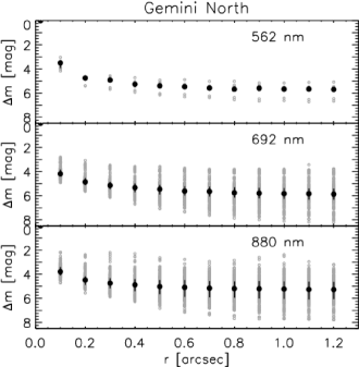
Figure 12: Image sensitivities for observations of Kepler stars with the Gemini 8-m telescope. The median sensitivities and quartiles are plotted with black symbols. The median FWHM of the stellar images was 0.02″.

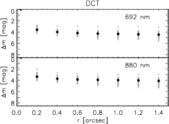
Figure 13: Image sensitivities for observations of Kepler stars with the DCT 4-m telescope. The median sensitivities and quartiles are plotted with black symbols. The median FWHM of the stellar images was 0.04″.

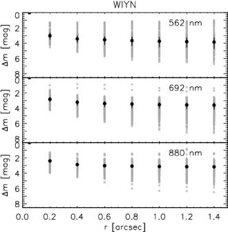
Figure 14: Image sensitivities for observations of Kepler stars with the WIYN 3.5-m telescope. The median sensitivities and quartiles are plotted with black symbols. The median FWHM of the stellar images was 0.05″.

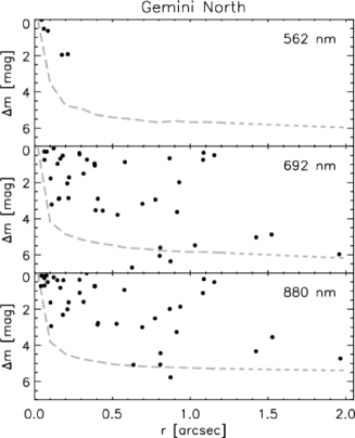
Figure 15: Magnitude difference versus radial separation for all companions detected around Kepler stars with the Gemini 8-m telescope at 562 nm (top), 692 nm (middle), and 880 nm (bottom). The dashed lines are the median image sensitivities from Figure 12.

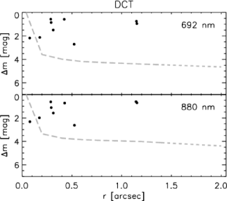
Figure 16: Magnitude difference versus radial separation for all companions detected around Kepler stars with the DCT 4-m telescope at 692 nm (top) and 880 nm (bottom). The dashed lines are the median image sensitivities from Figure 13.

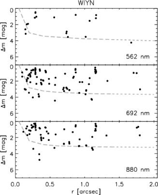
Figure 17: Magnitude difference versus radial separation for all companions detected around Kepler stars with the WIYN 3.5-m telescope at 562 nm (top), 692 nm (middle), and 880 nm (bottom). Some repeated observations of the same star result in points stacked at the same position. The dashed lines are the median image sensitivities from Figure 14.

As with the AO data, we measured image sensitivities and the separations, position angles, and brightness differences for any companions detected in the speckle images (note that the field of view of these images is much smaller than for the AO images). The 5$\sigma$ sensitivity limits are shown in Figures 12 to 14. The FWHM of the stellar PSFs were 0.02″ at Gemini North, 0.04″ at the DCT, and 0.05″ at WIYN (see Table 6). The sensitivity to companions is relatively flat from about 0.3″ to the edge of the field of view (about 1.4″ from the central star), and it is lower than the sensitivity of the Keck and Palomar AO images. However, within $\sim$ 0.2″ speckle interferometry is more sensitive to companions than adaptive optics (median $\Delta m\sim$ 4-5 in all three bands at Gemini North). Compared to the image sensitivities from Horch et al. (2014), who used a subsample of the speckle data from Gemini North and WIYN presented in this work, our values for the WIYN 692 nm data are very similar, while our values for the Gemini North 692 nm data are somewhat different. For the latter, our sensitivities are about 1 magnitude worse below 0.4″ and between 1.5 and 2.5 magnitudes less sensitive in the 0.4″-1.2″ range. This is likely a result of the larger sample studied here (158 vs. 35 stars in Horch et al. 2014) and thus a wider range of observing conditions.

Companions detected in speckle images are shown in Figures 15 to 17; each individual detection is shown. In some cases a target was observed at the same facility with the same filter multiple times, resulting in more than one measurement for a certain companion; these multiple measurements disagree in a few cases by up to $\sim$ 0.5 mag (see Fig. 17), likely a result of different observing conditions. At both Gemini North and WIYN, targets were typically observed at 692 and 880 nm, with some targets also observed at 562 nm, while at DCT only the 692 and 880 nm filters were used. We find at least one companion within the field of view ($\sim$ 2″) around 39 of the 158 unique KOI host stars observed at Gemini North; this fraction is 7 out of 75 for the KOI stars observed at DCT and 49 out of 681 for the KOI stars observed at WIYN (see Table 7). Except for two KOI host stars, multiple systems discovered in speckle images are binaries; only KOI 2626 and 2032 have two companions detected in Gemini North speckle images, and thus, if bound, they would form triple stellar systems.

Overall, at the three telescopes where DSSI was used, 828 unique KOI host stars were observed; of these, 85 have at least one companion detected within $\sim$ 2″. This translates to an observed fraction of multiple stellar systems in our speckle sample of 10$\pm$1%. If we consider only companions within 1″ of the primary star, we find that the observed fraction of multiple stellar systems is 8$\pm$1%. These fractions are smaller than what we found from our AO data for companions within 4″, which is a result of the smaller field of view of the speckle images. If we only consider companions detected at separations $\leq$ 1″, 10$\pm$1% of KOI host stars observed with AO have companions (79 out of 770 stars), which is in agreement with the results from speckle imaging. The same fraction, 10$\pm$1%, also results when combining the samples of stars we targeted with AO and speckle imaging (116 out of a total of 1189 unique KOI host stars have at least one companion within 1″).

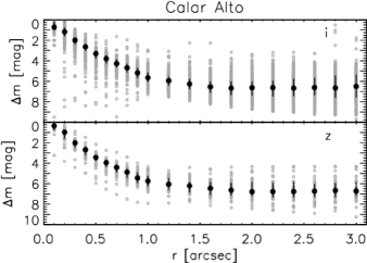
Figure 18: Image sensitivities for observations of Kepler stars with the Calar Alto 2.2-m telescope. The median sensitivities and quartiles are plotted with black symbols.

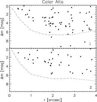
Figure 19: Magnitude difference versus radial separation for all companions detected around Kepler stars with the Calar Alto 2.2-m telescope in the $i$-band (top) and $z$-band (bottom). The dashed lines are the median image sensitivities from Figure 18.

4.1.3 Calar Alto

Lillo-Box et al. (2012, 2014) used the lucky imaging technique to obtain high-resolution images for a sample of 234 KOI host stars. Given that this imaging method is different from the ones described above, we include in this section image sensitivity plots for the images taken with the SDSS $i$ and $z$ filters and the AstraLux instrument (the data can be found on the CFOP site). The 5$\sigma$ sensitivities are shown in Figure 18; beyond about 1″, they are somewhat lower than the sensitivities of most of our AO images (median $\Delta m\sim$ 6-7 versus median $\Delta m>$ 8 for the AO $K$-band data), but they are substantially lower in the inner 0.5″. This is not surprising, given the different imaging techniques.

The companions detected within 4″ by Lillo-Box et al. (2012, 2014) are shown in Figure 19. Only a few bright companions are found within $\sim$ 1″, but several fainter companions ($\Delta m\sim$ 4-6) are revealed at separations larger than about 2″. In this separation range, there are a few companions with $\Delta m$ of 7-9.5 in the $i$-band (these detections lie above the median image sensitivity since the images used to extract them were likely obtained under exceptionally good observing conditions). Of the 234 KOI host stars observed, 53 have at least one companion at projected separations $<$ 4″, which translates to an observed fraction of 23$\pm$3%, a value just somewhat lower than the one derived from our AO data. If only companions within 1″ are considered, the observed fraction of stars with companions decreases to 3$\pm$1%. This value is much smaller than what we obtained from our AO and speckle images and can be understood in terms of the lower image sensitivity of the lucky images within $\sim$ 1″ from the primary stars.

4.2 Compilation of all KOI Host Star Companions

We combined the results on detected KOI companions from this work and the literature (see Table 1 for references) to create a list with the separations and position angles of the companions and any $\Delta m$ values that were measured (including their derived uncertainties, but with a floor of 0.01 mag). We limit this list to companions within 4″ of each KOI host star. It is important to note that the companions are not necessarily bound; they could be background stars or galaxies that are just by chance aligned with a KOI host star, and more analysis is needed to determine whether they and their primary stars form bound systems (see Teske et al., 2015; Hirsch et al., 2016). On the other hand, from simulations of stars in the Kepler field, Horch et al. (2014) found that most of the companions within $\sim$ 1″ are expected to be bound.

When combining the measurements of detected companions, we used results from both high-resolution imaging and seeing-limited imaging (mainly the UKIRT survey). Some companions were detected in only one band, while others have detections in multiple bands. For the separation and position angle of each companion, we averaged the results from different measurements; they usually agreed fairly well, but in a few cases the position angles were discrepant (usually related to an orientation problem in the image). When companions were measured multiple times in the same band, we averaged their $\Delta m$ values in that band, weighted by the inverse squared of the uncertainty in $\Delta m$ of each measurement. If the standard deviation of the individual measurements was larger than the formal value of the combined $\Delta m$ uncertainties, we used it as the uncertainty of the average $\Delta m$ value. Thus, in a few cases where the measurements were discrepant, the uncertainty of the combined $\Delta m$ value is fairly large.

The results of our KOI companion compilation are shown in Table 8. It contains 2297 companions around 1903 primary stars; 330 KOI host stars have two or more companions stars. We assign an identifier to each companion, choosing letters “B” to “H” for the first to seventh companion star. This nomenclature does not imply that the companions are actually bound (see note above); it is used to uniquely identify each companion star. There are eight KOI host stars with more than three companions: KOI 113, 908, 1019, 1397, 1884, 3049, 3444, and 4399; most of these companions lie at separations $>$1″ and may therefore be unbound. We also list the KIC ID for each primary and companion star in Table 8; in most cases, the two KIC IDs are the same, since the stars are not resolved in the KIC, but for 78 wide companions ($\geq$ 2″ from the primary), both objects can be found in the KIC.

Table 8: Relative Photometry (${\Delta}m$), Separations and Position Angles for Companions to KOI Host Stars

						$\Delta m=m_{\mathrm{secondary}}-m_{\mathrm{primary}}$ for photometric bands:
KOI	ID	KICIDprim	KICIDsec	d [$\arcsec$]	PA [°]	$F555W$	$F775W$	$i$	$z$	$LP600$	$562$	$692$	$880$
(1)	(2)	(3)	(4)	(5)	(6)	(7)	(8)	(9)	(10)	(11)	(12)	(13)	(14)
1	B	11446443	(11446443)	1.112 $\pm$ 0.051	136.2 $\pm$ 1.1	$\cdots$	$\cdots$	3.950 $\pm$ 0.330	$\cdots$	$\cdots$	$\cdots$	4.269 $\pm$ 0.150	3.379 $\pm$ 0.150
2	B	10666592	(10666592)	3.093 $\pm$ 0.050	266.4 $\pm$ 1.0	$\cdots$	$\cdots$	$\cdots$	$\cdots$	$\cdots$	$\cdots$	$\cdots$	$\cdots$
2	C	10666592	(10666592)	3.849 $\pm$ 0.060	90.1 $\pm$ 1.1	$\cdots$	$\cdots$	$\cdots$	$\cdots$	$\cdots$	$\cdots$	$\cdots$	$\cdots$
4	B	3861595	(3861595)	3.394 $\pm$ 0.062	74.8 $\pm$ 1.0	$\cdots$	$\cdots$	4.460 $\pm$ 0.050	$\cdots$	$\cdots$	$\cdots$	$\cdots$	$\cdots$
5	B	8554498	(8554498)	0.029 $\pm$ 0.050	142.1 $\pm$ 1.0	$\cdots$	$\cdots$	$\cdots$	$\cdots$	$\cdots$	$\cdots$	$\cdots$	$\cdots$
5	C	8554498	(8554498)	0.141 $\pm$ 0.050	304.3 $\pm$ 2.2	$\cdots$	$\cdots$	$\cdots$	$\cdots$	$\cdots$	2.841 $\pm$ 0.389	3.036 $\pm$ 0.150	$\cdots$
6	B	3248033	(3248033)	3.381 $\pm$ 0.050	307.8 $\pm$ 1.0	$\cdots$	$\cdots$	$\cdots$	$\cdots$	$\cdots$	$\cdots$	$\cdots$	$\cdots$
10	B	6922244	(6922244)	3.128 $\pm$ 0.050	265.8 $\pm$ 1.0	$\cdots$	$\cdots$	$\cdots$	$\cdots$	$\cdots$	$\cdots$	$\cdots$	$\cdots$
10	C	6922244	(6922244)	3.830 $\pm$ 0.050	89.3 $\pm$ 1.0	$\cdots$	$\cdots$	$\cdots$	$\cdots$	$\cdots$	$\cdots$	$\cdots$	$\cdots$
12	B	5812701	(5812701)	0.603 $\pm$ 0.050	345.7 $\pm$ 1.0	$\cdots$	$\cdots$	$\cdots$	$\cdots$	$\cdots$	$\cdots$	$\cdots$	$\cdots$
12	C	5812701	(5812701)	1.903 $\pm$ 0.050	320.3 $\pm$ 1.0	$\cdots$	$\cdots$	$\cdots$	$\cdots$	$\cdots$	$\cdots$	$\cdots$	$\cdots$
13	B	9941662	(9941662)	1.144 $\pm$ 0.083	279.7 $\pm$ 4.3	$\cdots$	$\cdots$	0.190 $\pm$ 0.060	$\cdots$	$\cdots$	1.008 $\pm$ 0.276	0.715 $\pm$ 0.210	0.619 $\pm$ 0.239
14	B	7684873	(7684873)	1.724 $\pm$ 0.050	273.5 $\pm$ 1.0	$\cdots$	$\cdots$	$\cdots$	$\cdots$	$\cdots$	$\cdots$	$\cdots$	$\cdots$
18	B	8191672	(8191672)	0.912 $\pm$ 0.050	167.3 $\pm$ 1.0	$\cdots$	$\cdots$	$\cdots$	$\cdots$	$\cdots$	$\cdots$	$\cdots$	$\cdots$
18	C	8191672	(8191672)	3.464 $\pm$ 0.050	110.5 $\pm$ 1.1	$\cdots$	$\cdots$	$\cdots$	$\cdots$	$\cdots$	$\cdots$	$\cdots$	$\cdots$
21	B	10125352	10125357	2.074 $\pm$ 0.050	59.8 $\pm$ 1.0	$\cdots$	$\cdots$	$\cdots$	$\cdots$	$\cdots$	$\cdots$	$\cdots$	$\cdots$
28	B	4247791	(4247791)	0.560 $\pm$ 0.050	23.3 $\pm$ 1.0	$\cdots$	$\cdots$	$\cdots$	$\cdots$	$\cdots$	1.110 $\pm$ 0.150	$\cdots$	$\cdots$
41	B	6521045	(6521045)	1.832 $\pm$ 0.050	242.1 $\pm$ 1.0	$\cdots$	$\cdots$	4.206 $\pm$ 0.097	$\cdots$	$\cdots$	$\cdots$	$\cdots$	$\cdots$
41	C	6521045	(6521045)	3.434 $\pm$ 0.050	195.8 $\pm$ 1.0	$\cdots$	$\cdots$	$\cdots$	$\cdots$	$\cdots$	$\cdots$	$\cdots$	$\cdots$
42	B	8866102	(8866102)	1.667 $\pm$ 0.061	35.7 $\pm$ 2.1	$\cdots$	$\cdots$	$\cdots$	$\cdots$	3.040 $\pm$ 0.170	4.240 $\pm$ 0.150	$\cdots$	$\cdots$
43	B	9025922	(9025922)	3.341 $\pm$ 0.050	83.6 $\pm$ 1.0	$\cdots$	$\cdots$	$\cdots$	$\cdots$	$\cdots$	$\cdots$	$\cdots$	$\cdots$
44	B	8845026	(8845026)	3.356 $\pm$ 0.068	124.7 $\pm$ 1.3	$\cdots$	$\cdots$	$\cdots$	$\cdots$	$\cdots$	$\cdots$	$\cdots$	$\cdots$
45	B	3742855	(3742855)	3.140 $\pm$ 0.050	36.8 $\pm$ 1.0	$\cdots$	$\cdots$	$\cdots$	$\cdots$	$\cdots$	$\cdots$	$\cdots$	$\cdots$
45	C	3742855	(3742855)	3.964 $\pm$ 0.051	72.9 $\pm$ 2.3	$\cdots$	$\cdots$	$\cdots$	$\cdots$	$\cdots$	$\cdots$	$\cdots$	$\cdots$
51	B	6056992	(6056992)	3.510 $\pm$ 0.050	161.0 $\pm$ 1.0	$\cdots$	$\cdots$	$\cdots$	$\cdots$	2.630 $\pm$ 0.070	$\cdots$	$\cdots$	$\cdots$
53	B	2445975	2445980	3.315 $\pm$ 0.050	95.5 $\pm$ 1.0	$\cdots$	$\cdots$	$\cdots$	$\cdots$	$\cdots$	$\cdots$	$\cdots$	$\cdots$
53	C	2445975	2445972	3.381 $\pm$ 0.050	210.9 $\pm$ 1.0	$\cdots$	$\cdots$	$\cdots$	$\cdots$	$\cdots$	$\cdots$	$\cdots$	$\cdots$
68	B	8669092	(8669092)	0.735 $\pm$ 0.052	256.5 $\pm$ 2.1	$\cdots$	$\cdots$	$\cdots$	$\cdots$	$\cdots$	3.131 $\pm$ 0.348	2.874 $\pm$ 0.150	$\cdots$
68	C	8669092	(8669092)	2.738 $\pm$ 0.060	256.7 $\pm$ 4.0	$\cdots$	$\cdots$	$\cdots$	$\cdots$	$\cdots$	$\cdots$	$\cdots$	$\cdots$
68	D	8669092	(8669092)	3.406 $\pm$ 0.053	352.4 $\pm$ 3.6	$\cdots$	$\cdots$	$\cdots$	$\cdots$	$\cdots$	$\cdots$	$\cdots$	$\cdots$

Note. — Column (1) lists the KOI number of the host star, column (2) the identifier we assigned to each companion star (“B” for the first companion, “C” for the second companion, etc), columns (3) and (4) contain the KIC ID of the primary and companion (“secondary”) star, respectively (a value in parentheses for the companion star means that it is not a distinct source in the KIC), columns (5) and (6) list the separation and position angle (from north through east), respectively, of the companion relative to the primary, and columns (7) to (20) list the difference in magnitudes between the primary and the companion star in different bands.

Table 8: Continued. Relative Photometry (${\Delta}m$), Separations and Position Angles for Companions to KOI Host Stars

		$\Delta m=m_{\mathrm{secondary}}-m_{\mathrm{primary}}$ for photometric bands:
KOI	ID	$U$	$B$	$V$	$J$	$H$	$K$
(1)	(2)	(15)	(16)	(17)	(18)	(19)	(20)
1	B	$\cdots$	$\cdots$	$\cdots$	2.800 $\pm$ 0.100	2.500 $\pm$ 0.100	2.359 $\pm$ 0.029
2	B	$\cdots$	$\cdots$	$\cdots$	$\cdots$	$\cdots$	7.525 $\pm$ 0.114
2	C	$\cdots$	$\cdots$	$\cdots$	5.745 $\pm$ 0.018	$\cdots$	5.965 $\pm$ 0.045
4	B	$\cdots$	$\cdots$	$\cdots$	4.233 $\pm$ 0.010	$\cdots$	$\cdots$
5	B	$\cdots$	$\cdots$	$\cdots$	$\cdots$	$\cdots$	0.400 $\pm$ 0.062
5	C	$\cdots$	$\cdots$	$\cdots$	$\cdots$	$\cdots$	2.310 $\pm$ 0.199
6	B	$\cdots$	$\cdots$	$\cdots$	7.393 $\pm$ 0.126	$\cdots$	$\cdots$
10	B	$\cdots$	$\cdots$	$\cdots$	7.895 $\pm$ 0.032	$\cdots$	$\cdots$
10	C	$\cdots$	$\cdots$	$\cdots$	6.266 $\pm$ 0.032	$\cdots$	$\cdots$
12	B	$\cdots$	$\cdots$	$\cdots$	$\cdots$	$\cdots$	3.835 $\pm$ 0.010
12	C	$\cdots$	$\cdots$	$\cdots$	$\cdots$	$\cdots$	7.539 $\pm$ 0.043
13	B	$\cdots$	$\cdots$	$\cdots$	0.180 $\pm$ 0.031	$\cdots$	0.145 $\pm$ 0.042
14	B	$\cdots$	$\cdots$	$\cdots$	4.304 $\pm$ 0.150	$\cdots$	3.514 $\pm$ 0.150
18	B	$\cdots$	$\cdots$	$\cdots$	5.365 $\pm$ 0.041	$\cdots$	$\cdots$
18	C	$\cdots$	$\cdots$	$\cdots$	6.014 $\pm$ 0.122	$\cdots$	$\cdots$
21	B	$\cdots$	$\cdots$	$\cdots$	2.402 $\pm$ 0.010	$\cdots$	$\cdots$
28	B	$\cdots$	$\cdots$	$\cdots$	$\cdots$	$\cdots$	$\cdots$
41	B	$\cdots$	$\cdots$	$\cdots$	$\cdots$	$\cdots$	$\cdots$
41	C	$\cdots$	$\cdots$	$\cdots$	$\cdots$	$\cdots$	10.049 $\pm$ 0.162
42	B	$\cdots$	$\cdots$	$\cdots$	2.212 $\pm$ 0.026	$\cdots$	1.873 $\pm$ 0.024
43	B	1.199 $\pm$ 0.065	1.135 $\pm$ 0.049	1.098 $\pm$ 0.034	1.110 $\pm$ 0.016	$\cdots$	$\cdots$
44	B	$\cdots$	$\cdots$	$\cdots$	3.983 $\pm$ 0.021	3.803 $\pm$ 0.032	3.825 $\pm$ 0.010
45	B	$\cdots$	$\cdots$	$\cdots$	1.407 $\pm$ 0.087	$\cdots$	$\cdots$
45	C	$\cdots$	$\cdots$	$\cdots$	-2.503 $\pm$ 0.021	-2.092 $\pm$ 0.151	$\cdots$
51	B	$\cdots$	$\cdots$	$\cdots$	$\cdots$	$\cdots$	$\cdots$
53	B	-0.952 $\pm$ 0.035	-0.579 $\pm$ 0.036	-0.378 $\pm$ 0.027	-0.099 $\pm$ 0.010	$\cdots$	$\cdots$
53	C	1.170 $\pm$ 0.047	0.695 $\pm$ 0.037	0.500 $\pm$ 0.028	-0.295 $\pm$ 0.010	$\cdots$	$\cdots$
68	B	$\cdots$	$\cdots$	$\cdots$	2.025 $\pm$ 0.070	$\cdots$	1.800 $\pm$ 0.020
68	C	$\cdots$	$\cdots$	$\cdots$	7.166 $\pm$ 0.090	$\cdots$	6.200 $\pm$ 0.020
68	D	$\cdots$	$\cdots$	$\cdots$	6.498 $\pm$ 0.229	$\cdots$	5.800 $\pm$ 0.020

Note. — The full table is available in a machine-readable form in the online journal. A portion is shown here for guidance regarding content and form.

The companions from Table 8 are plotted in Figures 20 and 21. The two figures separate the KOIs identified as planet candidates or confirmed planets from those identified as false positives (if a KOI host star has both candidate or confirmed planets and one or more false positive transit signals, its companions are shown in Figure 20). Both Figures 20 and 21 show the difference in magnitudes between primary and companion versus their projected separations, color-coded by the different photometric bands (some are grouped into the same color). Thus, if a companion has been detected in more than one photometric band, it will appear more than once in the figure, but usually with a different color and also likely different $\Delta m$ value. Speckle and AO find the closest companions, while AO, lucky imaging, and in particular HST imaging find the faintest companions. Robo-AO imaging detects companions down to 0.2″, with typical $\Delta m$ values (mostly in the $LP600$ band) between 0 and 5; just $\sim$ 8% of companions found with Robo-AO are fainter than the primary by $\geq$ 5 mag. The UKIRT survey detects most companions at separations between 2″ and 4″ (and beyond); typical $\Delta J$ values are below 7 mag.

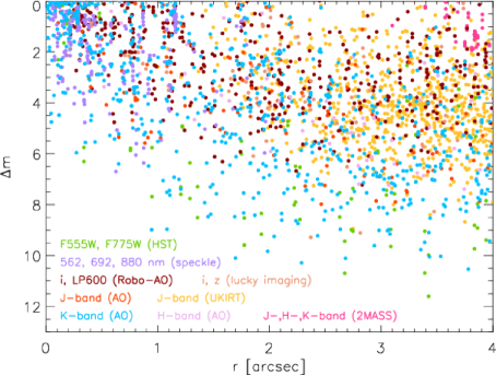
Figure 20: Magnitude difference versus radial projected separation relative to the primary star for all companions detected around Kepler planet host stars (i.e., stars that host at least one candidate or confirmed planet). The magnitude differences in the various photometric bands are color-coded.

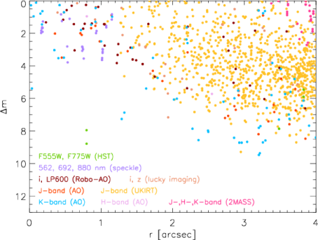
Figure 21: Magnitude difference versus radial projected separation relative to the primary star for all companions detected around Kepler stars with one or more transit events that are all classified as false positive.

Figure 22 shows the distribution of projected separations between primary stars and companions for all KOI host stars. Also shown are histograms for the separations of companions detected only in UKIRT data (some of these stars are also detected in 2MASS and UBV survey data) and of companions detected also (or only) in high-resolution imaging data. The increase in numbers for separations larger than about 1.6″ is clearly due to the detections of companions in UKIRT images. It is likely that many of these stars are not actually bound companions, but background stars or galaxies. Of the companions detected in high-resolution imaging data (thus, excluding companions detected only in UKIRT, 2MASS, and UBV survey data), we find that 46$\pm$2% are found at separations $<$ 2″; of these close companions, 53$\pm$3% are within 1″ from the primary.

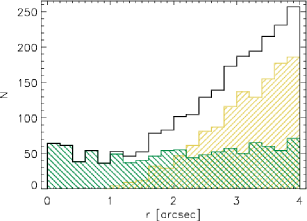
Figure 22: Histogram of the distribution of radial projected separations for all detected companions to KOI host stars (black line). The yellow shaded histogram is the distribution of companion separations for companions detected only in UKIRT (and sometimes also 2MASS and UBV survey images), while the green shaded histogram is for the remaining companions detected in high-resolution images.

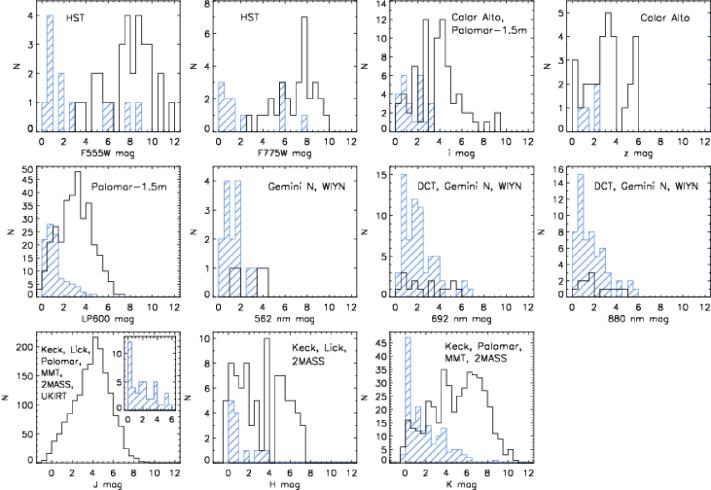
Figure 23: Histograms of the distributions of $\Delta m$ values in various bands for all detected companions to KOI host stars. The blue shaded histogram is the distribution for companions separated by $\leq$ 1″ from the primary star, while the black histograms are for companions separated by $>$ 1″.

The distributions of $\Delta m$ values in various bands for all detected companions to KOI host stars are shown in Figure 23. The most sensitive observations are those obtained by HST; a few companions have $\Delta m>10$ in the $F555W$ band. Of the ground-based observations at optical wavelengths, the faintest companions are detected in the $i$-band with lucky imaging at Calar Alto. The three bands with the largest number of observations and thus companion detections, $LP600$, $J$, and $K$ display different distributions of $\Delta m$ values for companions at $>$ 1″ from the primary stars. The $LP600$ band shows a broad peak around 3.5 mag, while the $K$-band distribution is very wide, spanning values up to 11 mag, with two peaks at 4 and 7 mag and smaller peaks at 0 and 2.5 mag. The $J$ band, which is dominated by UKIRT measurements, displays a broad peak centered at 4-4.5 mag.

Of particular interest are companions detected within 1″ from the primary. Most of these companions are not much fainter than the primary ($\Delta m<2$); this is partly an observational effect, as very faint companions next to brighter stars can be difficult to detect. At near-infrared wavelengths ($J$, $H$, $K$ bands), most close companions have $\Delta m$=0-0.5. In the $K$ band, almost all companions at $\leq$ 1″ and with $\Delta K$ $<$ 0.5 were detected at Keck with adaptive optics. It is these bright, close companions that will have the largest effect on derived planet radii, as is described in the next section.

4.3 Revised Transit Depths and Planet Radii

4.3.1 Background

The observed transit depth $\delta_{\rm obs}$ in the Kepler bandpass ($Kp$) is used to derive planet radii:

$$\delta_{\rm obs}=\frac{F_{\rm tot}-F_{\rm transit}}{F_{\rm tot}}=\left(\frac{R_{p}}{R_{\ast}}\right)^{2},$$ (1)

where $F_{\rm tot}$ is the total out-of-transit flux, $F_{\rm transit}$ is the in-transit flux, and $R_{p}$ and $R_{\ast}$ are the planet and stellar radius, respectively. However, if there is more than one star in a system, the total flux is the sum of the stellar fluxes, but the in-transit flux depends on which star the planet transits. Thus, the observed transit depth becomes

$$\delta_{\rm obs}=\left(\frac{F_{\ast}}{F_{\rm tot}}\right)\left(\frac{R_{p}}{R_{\ast}}\right)^{2},$$ (2)

where the star symbol denotes the star with the transiting planet. Thus, the transit depth is shallower, and the derived planet radius is smaller when the additional stars in the system are not taken into account. Given that the radii of Kepler planets are derived assuming a single star (with a correction factor applied to account only for flux dilution by nearby stars resolved in the KIC; Mullally et al. 2015; Coughlin et al. 2016), the presence of close companions results in an upward revision of the planet radius (see Ciardi et al. 2015 for more details). If we assume that the planet orbits the primary star in a multiple system, the “corrected” planet radius relative to the one derived assuming a single star ($R_{p}$) is

$$R_{p,\rm corr}=R_{p}\sqrt{\frac{F_{\rm tot}}{F_{\rm prim}}},$$ (3)

where $F_{\rm tot}$ is the combined out-of-transit flux of all stars in the system and $F_{\rm prim}$ is the flux of the primary star. For two stars, $F_{\rm tot}=F_{\rm prim}+F_{\rm sec}$ and, in magnitudes, $\Delta m=m_{\rm sec}-m_{\rm prim}=-2.5\log(F_{\rm sec}/F_{\rm prim})$; then the previous equation becomes:

$$R_{p,\rm corr}=R_{p}\sqrt{1+10^{-0.4\Delta m}}$$ (4)

The expression under the square root can be considered a “planet radius correction factor”. For more than one companion star, the previous equation converts to

$$R_{p,\rm corr}=R_{p}\sqrt{1+\sum_{i=1}^{N}{10^{-0.4\Delta m_{i}}}},$$ (5)

where the sum is for N companion stars with magnitude differences $\Delta m_{i}$ relative to the primary star.

These equations for calculating revised planet radii assume that planets orbit the primary star; if they orbit one of the companion stars, there is an additional dependence on stellar radii:

$$R_{p,\rm corr}=R_{p}\frac{R_{\rm sec}}{R_{\ast}}\sqrt{\frac{F_{\rm tot}}{F_{\rm sec}}},$$ (6)

where $R_{sec}$ and $F_{sec}$ are the radius and flux, respectively, of the secondary star around which the planet orbits, and $R_{\ast}$ is the radius of the star when assumed to be single (i.e., the radius of the primary star). In the case of two stars, the flux ratio $F_{\rm tot}/F_{\rm sec}$ is equal to $1+10^{0.4\Delta m}$, where $\Delta m=m_{\rm sec}-m_{\rm prim}$. If there is more than one companion star and the planet obits the secondary whose magnitude difference with respect to the primary is $\Delta m_{c}$, the equation to derive revised planet radii becomes

$$R_{p,\rm corr}=R_{p}\frac{R_{\rm sec}}{R_{\ast}}\sqrt{10^{0.4\Delta m_{c}}(1+\sum_{i=1}^{N}{10^{-0.4\Delta m_{i}}})}$$ (7)

Thus, as shown by Ciardi et al. (2015), the radius correction factor can become much larger if planets orbit a typically fainter (and smaller) companion star.

The $\Delta m_{i}$ values in Equations 5 and 7 are for the Kepler bandpass. Thus, to revise the transit depths and thus planet radii for the systems in Table 8, the magnitude differences between primary stars and companions have to be converted from the bandpass in which they were measured to the equivalent magnitude difference in the Kepler bandpass.

For the HST F555W and F775W bandpasses, Cartier et al. (2015) derived the following relation:

$$Kp=0.236+0.406\times F555W+0.594\times F775W,$$ (8)

with an uncertainty in the derived $Kp$ value of $\sigma(Kp)=\sqrt{0.019^{2}(F555W-F775W)^{2}+0.027^{2}}$.

Lillo-Box et al. (2014) found a linear correlation between the Kepler magnitudes (for $13<Kp<16$) and the SDSS $i$ ($i_{SDSS}$) magnitudes:

$$i_{SDSS}=0.947Kp+0.510$$ (9)

Everett et al. (2015) used a library of model spectra to derive relationships between stellar properties and the conversion from magnitudes in the speckle filters to those in $Kp$. They then applied the conversion to each KOI host star based on the stellar properties reported for the star. As an approximation, we assume that magnitudes measured in the 692 nm DSSI band are the same as for the $Kp$ bandpass. Also the $LP600$ filter used by Robo-AO at the Palomar 1.5-m telescope is similar to the Kepler bandpass, and thus we can assume $\Delta LP600=\Delta Kp$ (Law et al., 2014; Baranec et al., 2016; Ziegler et al., 2016).

Howell et al. (2012) used photometry from the KIC and 2MASS magnitudes to derive relations between the infrared color $(J-K_{s})$ and the Kepler magnitude. They inferred

$$Kp-K_{s} = 0.314377+3.85667\Delta+3.176111\Delta^{2}$$

$$- 25.3126\Delta^{3}+40.7221\Delta^{4}$$

$$- 19.2112\Delta^{5}\quad\mathrm{for\;dwarfs}$$

$$Kp-K_{s} = 0.42443603+3.7937617\Delta-2.3267277\Delta^{2}$$ (10)

$$+ 1.4602553\Delta^{3}\mathrm{\quad for\;giants,}$$

where $\Delta=J-K_{s}$ (see Ciardi et al. 2011 on how dwarfs and giants are separated in the KIC). Typical uncertainties in the derived $Kp-K_{s}$ colors are 0.083 mag for dwarfs and 0.065 mag for giants. Given that, as in Howell et al. (2012), we measured the $K$-band magnitude of our targets in a band that is slightly different from the $K_{s}$ band, using the above relationships to convert our measured $K$-band magnitude to a $Kp$ magnitude adds an additional uncertainty of about 0.03 mag (see Howell et al., 2012).

For cases where only a $J$- or only a $K$-band magnitude is known, but not both, Howell et al. (2012) derived the following relations:

$$Kp-J = -398.04666+149.08127J-21.952130J^{2}$$

$$+ 1.5968619J^{3}-0.057478947J^{4}$$

$$+ 0.00082033223J^{5}$$

$$\mathrm{for} \mathrm{10\,mag<J<16.7\,mag}$$

$$Kp-J = 0.1918+0.08156J$$

$$\mathrm{for} \mathrm{J>16.7\,mag}$$

and

$$Kp-K_{s} = -643.05169+246.00603K_{s}-37.136501K_{s}^{2}$$

$$+ 2.7802622K_{s}^{3}-0.10349091K_{s}^{4}$$

$$+ 0.0015364343K_{s}^{5}$$

$$\mathrm{for} \mathrm{10\,mag<K_{s}<15.4\,mag}$$

$$Kp-K_{s} = -2.7284+0.3311K_{s}$$ (11)

$$\mathrm{for} \mathrm{K_{s}>15.4\,mag}$$

$Kp$ magnitude estimates using these equations have an uncertainty of about 0.6-0.8 mag.

4.3.2 Radius Correction Factors for Kepler Planets

Using the relations from Equations 8-11, we converted the measured $\Delta m$ values to $\Delta Kp$ values for observations in the $F555W$, $F775W$, $i$, $LP600$, 692 nm, $J$, and $K$ bands; of the 1903 KOI host stars that have nearby stars, just 12 do not have observations in any of these seven bands (and therefore do not have $\Delta Kp$ values derived for them). With $\Delta Kp$ for the companion stars, Equations 5 and 7 can be used to derive correction factors for the planet radii.

However, Equation 7 also requires the ratio of the stellar radii of the secondary and primary star. To derive an estimate of this ratio, we used the table with colors and effective temperatures for dwarf stars from Pecaut & Mamajek (2013) and assumed that primary and secondary stars are bound. We also assumed that $Kp$ magnitudes correspond to $R$ magnitudes, and we adopted effective temperatures ($T_{eff}$) for the primary stars from the stellar parameters of Huber et al. (2014). Using the tabulated $T_{eff}$ values, we derived $V-R$ ($=V-Kp$) colors and absolute $V$ magnitudes ($M_{V}$) for the primary stars. Assuming primary and secondary stars are bound and therefore at the same distance from the Sun implies $M_{V,\rm sec}=m_{V,\rm sec}-m_{V,\rm prim}+M_{V,\rm prim}$ or $M_{V,\rm sec}=Kp_{\rm sec}+(V-R)_{\rm sec}-Kp_{\rm prim}-(V-R)_{\rm prim}+M_{V,\rm prim}$. We found the $(V-R)_{\rm sec}$ color from the Pecaut & Mamajek (2013) table that yielded a self-consistent $M_{V,\rm sec}$ value. With $M_{V,\rm sec}$ determined, the effective temperature and luminosity of the secondary star are also known. Then, $\frac{R_{\rm sec}}{R_{\rm prim}}=\sqrt{\frac{L_{\rm sec}}{L_{\rm prim}}}\left(\frac{T_{eff,\rm prim}}{T_{eff,\rm sec}}\right)^{2}$. If a star had more than one companion within 4″, we adopted the $\frac{R_{\rm sec}}{R_{\rm prim}}$ ratio and $\Delta m_{c}$ value of the brightest companion star (highest luminosity as derived from its $M_{V}$ value) in Equation 7. We also checked that the brightness of the companion star, assumed to be bound to the primary star, was still consistent with the transit depth; for example, a transit depth of 0.1% is consistent with a companion star that is up to 7.5 mag fainter than the primary (in this case, the planet would fully obscure the companion star during transit). As a result, 249 companion stars were excluded from being the planet host star (roughly half of them are hosts to only false positive transit events).

For the 1891 KOI host stars with companions for which we derived $\Delta Kp$ values, we calculated factors to revise the planet radii to take the flux dilution into account. We derived such factors assuming the planets orbit the primary star (see Table 9) and assuming the planets orbit the brightest companion star (see Table 10). We included the small number of stars with companions resolved in the KIC; even though flux dilution by these companions should already be accounted for in the planet radii listed in the latest KOI table, we did not attempt to evaluate this correction term and decided to treat all companions uniformly. Both Tables 9 and 10 list correction factors derived from from measurements of $\Delta m$ in different bands; since the measurements were done in different filters at different telescopes, and there are uncertainties in converting them to $\Delta Kp$, the derived correction factors are expected to differ somewhat. Moreover, there are some cases in which a star has more than one companion, and not all companions are detected in all bands (for example, a faint companion close to the primary star is only detected in a Keck AO image, while a brighter companion at a larger distance is only measured in a UKIRT image). Therefore, radius correction factors, which depend on the sum of the $\Delta m_{i}$ values of the companion stars, are different for different bands for these stars.

We also computed a weighted average of the radius correction factors for each star by using the inverse of the square of the uncertainty as weight. Given that we derived up to four correction factors from the $J$- and $K$-band measurements, we used the individual correction factors derived from $J$- or $K$-band measurements if companions were only measured in one of these two bands. If measurements in both the $J$- and $K$-band were available, we instead used the average of the correction factors derived from the relationships between $J-K_{s}$ color and $Kp-K_{s}$ for dwarfs and giants. However, in Tables 9 and 10 there are 20 and 7 stars, respectively, for which the latter two correction factors differed by more than 25%; for these we used the correction factors derived from the $J-$ and $K$-band in our calculation of the weighted average. Also, for one star in Table 9 (KOI 2971), the radius correction factor derived from the $J$-band band was very close to 1 and discrepant with the values derived from the other bands (since only a more distant, faint companions was detected in $J$, but closer, brighter companions were detected in the other bands); the discrepant value was not included in the weighted average.

Table 9: Planet Radius Correction Factors Assuming Planets Orbit the Primary Stars, Derived from $\Delta m$ Measurements in Various Bands, and Weighted Average

KOI	F555W,F775W	i	692	LP600	J	K	$J-K$(dwarf)	$J-K$(giant)	Weighted average
(1)	(2)	(3)	(4)	(5)	(6)	(17)	(8)	(9)	(10)
1	$\cdots$	1.0107 $\pm$ 0.0034	1.0098 $\pm$ 0.0013	$\cdots$	1.0517 $\pm$ 0.0465	1.0810 $\pm$ 0.0650	1.0165 $\pm$ 0.0065	1.0193 $\pm$ 0.0057	1.0102 $\pm$ 0.0018
2	$\cdots$	$\cdots$	$\cdots$	$\cdots$	1.0029 $\pm$ 0.0024	1.0017 $\pm$ 0.0015	1.0033 $\pm$ 0.0002	1.0036 $\pm$ 0.0002	1.0034 $\pm$ 0.0002
4	$\cdots$	1.0065 $\pm$ 0.0003	$\cdots$	$\cdots$	1.0133 $\pm$ 0.0108	$\cdots$	$\cdots$	$\cdots$	1.0065 $\pm$ 0.0003
5	$\cdots$	$\cdots$	1.0301 $\pm$ 0.0041	$\cdots$	$\cdots$	1.3946 $\pm$ 0.3033	$\cdots$	$\cdots$	1.0301 $\pm$ 0.0041
6	$\cdots$	$\cdots$	$\cdots$	$\cdots$	1.0006 $\pm$ 0.0005	$\cdots$	$\cdots$	$\cdots$	1.0006 $\pm$ 0.0005
10	$\cdots$	$\cdots$	$\cdots$	$\cdots$	1.0013 $\pm$ 0.0011	$\cdots$	$\cdots$	$\cdots$	1.0013 $\pm$ 0.0011
12	$\cdots$	$\cdots$	$\cdots$	$\cdots$	$\cdots$	1.0215 $\pm$ 0.0175	$\cdots$	$\cdots$	1.0215 $\pm$ 0.0175
13	$\cdots$	1.3532 $\pm$ 0.0179	1.2319 $\pm$ 0.0407	$\cdots$	1.3555 $\pm$ 0.2605	1.3665 $\pm$ 0.2719	1.3301 $\pm$ 0.0233	1.3338 $\pm$ 0.0249	1.3314 $\pm$ 0.0226
14	$\cdots$	$\cdots$	$\cdots$	$\cdots$	1.0123 $\pm$ 0.0123	1.0295 $\pm$ 0.0291	1.0019 $\pm$ 0.0004	1.0026 $\pm$ 0.0006	1.0022 $\pm$ 0.0005
18	$\cdots$	$\cdots$	$\cdots$	$\cdots$	1.0047 $\pm$ 0.0042	$\cdots$	$\cdots$	$\cdots$	1.0047 $\pm$ 0.0042
21	$\cdots$	$\cdots$	$\cdots$	$\cdots$	1.0539 $\pm$ 0.0430	$\cdots$	$\cdots$	$\cdots$	1.0539 $\pm$ 0.0430
28	$\cdots$	$\cdots$	$\cdots$	$\cdots$	$\cdots$	$\cdots$	$\cdots$	$\cdots$	$\cdots$
41	$\cdots$	1.0083 $\pm$ 0.0008	$\cdots$	$\cdots$	$\cdots$	1.0000 $\pm$ 0.0000	$\cdots$	$\cdots$	1.0083 $\pm$ 0.0008
42	$\cdots$	$\cdots$	$\cdots$	1.0300 $\pm$ 0.0046	1.0174 $\pm$ 0.0144	1.0070 $\pm$ 0.0058	1.0405 $\pm$ 0.0044	1.0379 $\pm$ 0.0041	1.0349 $\pm$ 0.0044
43	$\cdots$	$\cdots$	$\cdots$	$\cdots$	1.1544 $\pm$ 0.1189	$\cdots$	$\cdots$	$\cdots$	1.1544 $\pm$ 0.1189
44	$\cdots$	$\cdots$	$\cdots$	$\cdots$	1.0125 $\pm$ 0.0104	1.0106 $\pm$ 0.0087	1.0093 $\pm$ 0.0011	1.0095 $\pm$ 0.0011	1.0094 $\pm$ 0.0011
45	$\cdots$	$\cdots$	$\cdots$	$\cdots$	3.6294 $\pm$ 1.3971	$\cdots$	$\cdots$	$\cdots$	3.6294 $\pm$ 1.3971
51	$\cdots$	$\cdots$	$\cdots$	1.0434 $\pm$ 0.0027	$\cdots$	$\cdots$	$\cdots$	$\cdots$	1.0434 $\pm$ 0.0027
53	$\cdots$	$\cdots$	$\cdots$	$\cdots$	1.8535 $\pm$ 0.5374	$\cdots$	$\cdots$	$\cdots$	1.8535 $\pm$ 0.5374
68	$\cdots$	$\cdots$	1.0348 $\pm$ 0.0047	$\cdots$	1.0854 $\pm$ 0.0736	1.1121 $\pm$ 0.0883	1.0567 $\pm$ 0.0108	1.0532 $\pm$ 0.0118	1.0378 $\pm$ 0.0057
69	$\cdots$	$\cdots$	$\cdots$	$\cdots$	$\cdots$	1.0000 $\pm$ 0.0000	$\cdots$	$\cdots$	1.0000 $\pm$ 0.0000
70	$\cdots$	$\cdots$	$\cdots$	$\cdots$	1.0093 $\pm$ 0.0076	1.0116 $\pm$ 0.0098	1.0055 $\pm$ 0.0005	1.0053 $\pm$ 0.0005	1.0054 $\pm$ 0.0005
72	$\cdots$	$\cdots$	$\cdots$	$\cdots$	$\cdots$	1.0005 $\pm$ 0.0005	$\cdots$	$\cdots$	1.0005 $\pm$ 0.0005
75	$\cdots$	$\cdots$	$\cdots$	$\cdots$	1.0012 $\pm$ 0.0011	1.0008 $\pm$ 0.0006	1.0008 $\pm$ 0.0003	1.0009 $\pm$ 0.0003	1.0008 $\pm$ 0.0003
84	$\cdots$	$\cdots$	$\cdots$	$\cdots$	$\cdots$	1.0000 $\pm$ 0.0000	$\cdots$	$\cdots$	1.0000 $\pm$ 0.0000
85	$\cdots$	$\cdots$	$\cdots$	$\cdots$	$\cdots$	1.0001 $\pm$ 0.0001	$\cdots$	$\cdots$	1.0001 $\pm$ 0.0001
97	$\cdots$	1.0056 $\pm$ 0.0028	$\cdots$	$\cdots$	1.0123 $\pm$ 0.0101	1.0093 $\pm$ 0.0077	1.0125 $\pm$ 0.0013	1.0125 $\pm$ 0.0013	1.0113 $\pm$ 0.0015
98	$\cdots$	1.3811 $\pm$ 0.0511	1.2436 $\pm$ 0.0512	$\cdots$	1.3233 $\pm$ 0.2461	1.3226 $\pm$ 0.2414	1.3359 $\pm$ 0.0468	1.3337 $\pm$ 0.0459	1.3174 $\pm$ 0.0493
99	$\cdots$	1.0002 $\pm$ 0.0001	$\cdots$	$\cdots$	1.0041 $\pm$ 0.0041	1.0032 $\pm$ 0.0027	1.0039 $\pm$ 0.0021	1.0040 $\pm$ 0.0018	1.0002 $\pm$ 0.0001
100	$\cdots$	$\cdots$	$\cdots$	$\cdots$	$\cdots$	$\cdots$	$\cdots$	$\cdots$	$\cdots$
102	$\cdots$	$\cdots$	$\cdots$	$\cdots$	1.1844 $\pm$ 0.1390	$\cdots$	$\cdots$	$\cdots$	1.1844 $\pm$ 0.1390
103	$\cdots$	$\cdots$	$\cdots$	$\cdots$	1.0003 $\pm$ 0.0005	1.0002 $\pm$ 0.0002	1.0001 $\pm$ 0.5044	1.0002 $\pm$ 0.0003	1.0002 $\pm$ 0.0002
105	$\cdots$	$\cdots$	$\cdots$	$\cdots$	1.0007 $\pm$ 0.0008	1.0162 $\pm$ 0.0132	1.0004 $\pm$ 0.0003	1.0004 $\pm$ 0.0002	1.0004 $\pm$ 0.0002

Note. — Column (1) lists the KOI number of the host star, columns (2)-(9) the radius correction factors calculated as shown in Equation 5, derived from ${\Delta}m$ measurements in different bands converted to $\Delta Kp$ values (see text for details), and column (10) the weighted average of the correction factors from the previous columns.

The full table is available in a machine-readable form in the online journal. A portion is shown here for guidance regarding content and form.

Table 10: Planet Radius Correction Factors Assuming Planets Orbit the Brightest Companion Stars, Derived from $\Delta m$ Measurements in Various Bands, and Weighted Average

KOI	ID	F555W,F775W	i	692	LP600	J	K	$J-K$(dwarf)	$J-K$(giant)	Weighted average
(1)	(2)	(3)	(4)	(5)	(6)	(17)	(8)	(9)	(10)	(11)
1	B	$\cdots$	3.305 $\pm$ 0.982	3.333 $\pm$ 0.864	$\cdots$	2.027 $\pm$ 0.911	1.682 $\pm$ 0.756	2.532 $\pm$ 0.751	2.386 $\pm$ 0.656	2.926 $\pm$ 0.819
2	C	$\cdots$	$\cdots$	$\cdots$	$\cdots$	$\cdots$	$\cdots$	$\cdots$	2.206 $\pm$ 0.560	2.206 $\pm$ 0.560
4	B	$\cdots$	3.622 $\pm$ 0.910	$\cdots$	$\cdots$	2.834 $\pm$ 1.262	$\cdots$	$\cdots$	$\cdots$	3.353 $\pm$ 1.030
5	B	$\cdots$	$\cdots$	$\cdots$	$\cdots$	$\cdots$	1.496 $\pm$ 0.742	$\cdots$	$\cdots$	1.496 $\pm$ 0.742
6	B	$\cdots$	$\cdots$	$\cdots$	$\cdots$	6.880 $\pm$ 3.094	$\cdots$	$\cdots$	$\cdots$	6.880 $\pm$ 3.094
10	C	$\cdots$	$\cdots$	$\cdots$	$\cdots$	$\cdots$	$\cdots$	$\cdots$	$\cdots$	$\cdots$
12	B	$\cdots$	$\cdots$	$\cdots$	$\cdots$	$\cdots$	2.288 $\pm$ 1.020	$\cdots$	$\cdots$	2.288 $\pm$ 1.020
13	B	$\cdots$	1.487 $\pm$ 0.375	1.574 $\pm$ 0.425	$\cdots$	1.487 $\pm$ 0.721	1.484 $\pm$ 0.724	1.487 $\pm$ 0.378	1.484 $\pm$ 0.377	1.511 $\pm$ 0.390
14	B	$\cdots$	$\cdots$	$\cdots$	$\cdots$	2.467 $\pm$ 1.114	1.938 $\pm$ 0.876	4.129 $\pm$ 1.084	3.688 $\pm$ 0.969	3.909 $\pm$ 1.028
18	B	$\cdots$	$\cdots$	$\cdots$	$\cdots$	$\cdots$	$\cdots$	$\cdots$	$\cdots$	$\cdots$
21	B	$\cdots$	$\cdots$	$\cdots$	$\cdots$	1.734 $\pm$ 0.775	$\cdots$	$\cdots$	$\cdots$	1.734 $\pm$ 0.775
28	B	$\cdots$	$\cdots$	$\cdots$	$\cdots$	$\cdots$	$\cdots$	$\cdots$	$\cdots$	$\cdots$
41	B	$\cdots$	3.604 $\pm$ 0.917	$\cdots$	$\cdots$	$\cdots$	$\cdots$	$\cdots$	$\cdots$	3.604 $\pm$ 0.917
42	B	$\cdots$	$\cdots$	$\cdots$	2.162 $\pm$ 0.566	2.811 $\pm$ 1.252	4.267 $\pm$ 1.900	1.860 $\pm$ 0.472	1.905 $\pm$ 0.484	1.999 $\pm$ 0.515
43	B	$\cdots$	$\cdots$	$\cdots$	$\cdots$	1.551 $\pm$ 0.709	$\cdots$	$\cdots$	$\cdots$	1.551 $\pm$ 0.709
44	B	$\cdots$	$\cdots$	$\cdots$	$\cdots$	3.109 $\pm$ 1.385	3.355 $\pm$ 1.494	2.464 $\pm$ 0.626	2.451 $\pm$ 0.623	2.457 $\pm$ 0.624
45	C	$\cdots$	$\cdots$	$\cdots$	$\cdots$	1.887 $\pm$ 1.111	$\cdots$	$\cdots$	$\cdots$	1.887 $\pm$ 1.111
51	B	$\cdots$	$\cdots$	$\cdots$	2.271 $\pm$ 0.572	$\cdots$	$\cdots$	$\cdots$	$\cdots$	2.271 $\pm$ 0.572
53	C	$\cdots$	$\cdots$	$\cdots$	$\cdots$	1.779 $\pm$ 0.945	$\cdots$	$\cdots$	$\cdots$	1.779 $\pm$ 0.945
68	B	$\cdots$	$\cdots$	2.030 $\pm$ 0.526	$\cdots$	1.591 $\pm$ 0.719	1.489 $\pm$ 0.673	1.640 $\pm$ 0.428	1.695 $\pm$ 0.445	1.815 $\pm$ 0.473
69	B	$\cdots$	$\cdots$	$\cdots$	$\cdots$	$\cdots$	$\cdots$	$\cdots$	$\cdots$	$\cdots$
70	B	$\cdots$	$\cdots$	$\cdots$	$\cdots$	3.522 $\pm$ 1.569	3.328 $\pm$ 1.483	2.778 $\pm$ 0.704	2.805 $\pm$ 0.711	2.791 $\pm$ 0.707
72	B	$\cdots$	$\cdots$	$\cdots$	$\cdots$	$\cdots$	7.718 $\pm$ 3.444	$\cdots$	$\cdots$	7.718 $\pm$ 3.444
75	B	$\cdots$	$\cdots$	$\cdots$	$\cdots$	5.705 $\pm$ 2.556	6.789 $\pm$ 3.024	3.664 $\pm$ 1.084	3.467 $\pm$ 0.951	3.566 $\pm$ 1.020
84	B	$\cdots$	$\cdots$	$\cdots$	$\cdots$	$\cdots$	$\cdots$	$\cdots$	$\cdots$	$\cdots$
85	B	$\cdots$	$\cdots$	$\cdots$	$\cdots$	$\cdots$	$\cdots$	$\cdots$	$\cdots$	$\cdots$
97	B	$\cdots$	3.816 $\pm$ 1.357	$\cdots$	$\cdots$	2.981 $\pm$ 1.328	3.302 $\pm$ 1.471	2.043 $\pm$ 0.518	2.043 $\pm$ 0.518	2.268 $\pm$ 0.625
98	B	$\cdots$	1.408 $\pm$ 0.372	1.424 $\pm$ 0.397	$\cdots$	1.393 $\pm$ 0.673	1.387 $\pm$ 0.668	1.331 $\pm$ 0.344	1.332 $\pm$ 0.344	1.383 $\pm$ 0.369
99	B	$\cdots$	$\cdots$	$\cdots$	$\cdots$	4.348 $\pm$ 1.963	4.748 $\pm$ 2.114	2.722 $\pm$ 0.927	2.693 $\pm$ 0.827	2.708 $\pm$ 0.878
100	B	$\cdots$	$\cdots$	$\cdots$	$\cdots$	$\cdots$	$\cdots$	$\cdots$	$\cdots$	$\cdots$
102	B	$\cdots$	$\cdots$	$\cdots$	$\cdots$	1.482 $\pm$ 0.682	$\cdots$	$\cdots$	$\cdots$	1.482 $\pm$ 0.682
103	B	$\cdots$	$\cdots$	$\cdots$	$\cdots$	$\cdots$	$\cdots$	$\cdots$	$\cdots$	$\cdots$
105	B	$\cdots$	$\cdots$	$\cdots$	$\cdots$	$\cdots$	3.053 $\pm$ 1.360	$\cdots$	$\cdots$	3.053 $\pm$ 1.360

Note. — Column (1) lists the KOI number of the host star, column (2) the identifier of the companion star (see Table 8) assumed to host the planet(s), columns (3)-(10) the radius correction factors calculated as shown in Equation 7, derived from ${\Delta}m$ measurements in different bands converted to $\Delta Kp$ values (see text for details), and column (10) the weighted average of the correction factors from the previous columns.

The full table is available in a machine-readable form in the online journal. A portion is shown here for guidance regarding content and form.

When assuming planets orbit the primary stars (Table 9), we find overall satisfactory agreement between the different radius correction factors for each KOI host star, especially considering the approximations involved in converting magnitude differences into the Kepler bandpass. The mean correction factors derived from the HST, $i$, $LP600$, and 692 nm bands are very similar, 1.072, 1.082, 1.102, and 1.114, respectively. Using just the $J$- and $K$-band magnitude differences individually, the mean correction factors derived from them are 1.053 and 1.101, respectively. When the $J-K$ colors are considered, assuming dwarf stars the average factor is 1.131, while it is 1.100 if giant stars are assumed. The somewhat larger correction factors for the $LP600$, 692 nm, and $K$-bands are related to the larger number of bright ($\Delta m<2$), close ($\leq$ 1″) companions detected in these bands (see Figure 23). Also, the correction factor for the $J$-band is somewhat lower since most companions in the $J$-band were detected by UKIRT, which mostly found more distant, fainter companions. As can be seen from Equation 5, an equal-brightness companion in a binary system results in a correction factor of 1.41, while the factor decreases to, e.g., 1.18, 1.08, and 1.03 for $\Delta m$ values of 1, 2, and 3 mag, respectively.

Under the assumption that planets orbit the brightest companion star (Table 10), the radius correction factors become larger. In this case, the mean correction factors derived from the HST, $i$, $LP600$, and 692 nm bands are 4.18, 2.75, 2.23, and 2.12, respectively. The average factors derived from the $J$- and $K$-band individually, and from the $J-K$-color relationship for dwarf and giant stars, are 3.21, 3.44, 2.31, and 2.25, respectively. Larger factors are due to fainter companions.

In Figures 24 and 25, we show the histograms of average planet radius correction factors for planets transiting KOI host stars that have at least one companion within 4″ detected in imaging observations (both high-resolution and seeing-limited). The correction factors in Figure 24 assume planets orbit the primary stars, while the factors in Figure 25 assume planets orbit the brightest companion stars. For all planets orbiting a certain KOI host star (primary or companion), the radius correction factor is the same, since it just depends on stellar properties (brightness ratios between primary and companion stars, and, for planets orbiting companion stars, ratios of stellar radii). Therefore, there is one planet radius correction factor per KOI host star. In Figures 24 and 25 we only include Kepler stars with companions that are hosts to planets, thus excluding those stars with only false positive events; this leaves 1036 stars in Fig. 24 (out of the 1891 stars for which we derived $\Delta Kp$ values), and 922 stars in Fig. 25 (out of the 1642 stars for which measured transit depths are still consistent with the brightness of the companion).

Figure 24: Histogram of the average planet radius correction factors derived from the measurements of detected companions to host stars of KOI planets in different bands, assuming that planets orbit the primary stars (one correction factor per star). There are six additional values between 1.54 and 1.86 that are not shown.

Figure 25: Histogram of the average planet radius correction factors derived from the measurements of detected companions to host stars of KOI planets in different bands, assuming that planets orbit the brightest companion stars (one correction factor per star). One additional value at 16.4 is not shown.

Assuming planets orbit the primary star, the mean and median planet radius correction factors for planet host stars are 1.06 and 1.01, respectively. There is a monotonic decrease in the frequency of correction factor values as the value increases. When assuming planets orbit the brightest companion star, the mean and median planet radius correction factors are 3.09 and 2.69, respectively; 90% of values are between 1.12 and 5.22, and just 18 stars have correction factors between 8.0 and the largest value, 16.4.

Figure 26: Histogram of the weighted average of planet radius correction factors shown in Figures 24 and 25 (see text for details).

If we calculate a weighted average of the planet radius correction factors, using weights of, e.g., 0.8 and 0.2 for the factors that assume planets orbit the primary stars and brightest companion stars, respectively, we derive a mean value of 1.47 and and a median value of 1.38. These weights exemplify the assumption that planets are more likely to orbit primary rather than secondary stars, since the former typically have more massive protoplanetary disks (e.g., Akeson & Jensen, 2014) which may lead to more efficient planet formation. Assuming that planets are equally likely to orbit the primary and secondary star, the mean and median correction factors increase somewhat to 2.08 and 1.85, respectively. The histogram of our weighted average correction factors is shown in Figure 26; three quarters of values are below 1.58. Therefore, in a more realistic scenario where most planets orbit the primary stars, but some orbit secondary stars, the average planet radius correction factors are typically $\lesssim$ 2. Our mean weighted average radius correction factor is very similar to the result from Ciardi et al. (2015), who modeled multiple stellar systems and derived that, on average, planet radii are underestimated by a factor of 1.5. However, we note that these average or median correction factors should not be applied to individual planets in multiple stellar systems to correct their radii; each system is unique, and the increase in radius is either relatively small, of the order of several percent, if a planet orbits the primary star (which is expected for many, if not most, planets), or of the order of a few if it is determined that the planet orbits a fainter companion star.

5 Discussion

5.1 Effect of Companions on Planet Radii

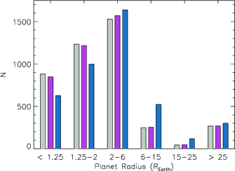
Figure 27: Histograms of planet radii of all KOI planet candidates and confirmed planets from the latest KOI cumulative table targeted by high-resolution imaging (gray) and the same planet radii, but corrected using the average radius correction factors for each star derived in section 4.3 assuming planets orbit the primary stars (purple) and assuming planets orbit the brightest companion stars (blue).

We applied the average radius correction factors for each star derived in the previous section to the radii of all those KOI planets whose host stars were targeted by high-resolution imaging and had a companion detected in the $F555W$, $F775W$, $i$, $LP600$, 692 nm, $J$, or $K$ bands (for stars without detected companions, the correction factor is 1). In Figure 27 we show the distributions of planet radii before and after applying correction factors; the planet radii are binned in ranges often used to group different classes of planets (e.g., super-Earths have $\sim$1.25-2 R_⊕, Neptunes have $\sim$ 2-6 R_⊕). When assuming that planets orbit the primary stars (purple bars in Fig. 27), there are only slight changes in the various histogram bins; the number of planets with radii from 0.5 to 2 R_⊕ decreases somewhat, while there are more planets in the 2-6 R_⊕ range. Under the assumption that planets orbit the brightest companion stars (blue bars in Fig. 27), the number of planets with radii from 0.5 to 2 R_⊕ decreases noticeably, while the number of planets with radii larger than 2 R_⊕ increases. Table 11 lists the number of planets in certain radius bins before and after the correction factors were applied to the planet radii.

Table 11: Number of KOI Planets in Different Radius Bins, Orbiting Stars Targeted by High-resolution Imaging

$R_{p}$ range (R⊕)	Nall	Nall,obs.	N${}_{\rm obs.,corr.}^{\rm prim}$	N${}_{\rm obs.,corr.}^{\rm sec}$
(1)	(2)	(3)	(4)	(5)
0.25 – 1.25	983	882	847	627
1.25 – 2.0	1337	1233	1217	999
2.0 – 6.0	1622	1529	1571	1638
6.0 – 15	297	249	253	522
15 – 25	73	43	47	117
$>$ 25	394	267	268	300

Note. — Column (1) lists the range for the planet radius, column (2) the number of KOI planets from the latest KOI cumulative table with radii within that radius range, columns (3), (4), and (5) the number of KOI planets from column (2) that were targeted by high-resolution imaging, split into the same radius ranges, but for the planets in column (3) no correction was applied to the radius, while for the planets in columns (4) and (5) the radii have been corrected with the average radius correction factors for each star assuming the planets orbit the primary or the brightest companion star, respectively (see text for details).

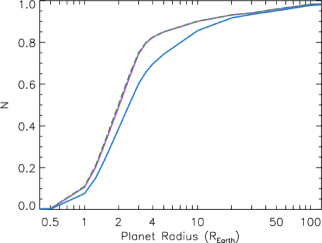
Figure 28: Cumulative distribution of planet radii of all KOI planet candidates and confirmed planets from the latest KOI cumulative table targeted by high-resolution imaging (green, dashed line) and the same planet radii, but corrected using the average radius correction factors for each star derived in section 4.3 assuming planets orbit the primary stars (purple) and assuming planets orbit the brightest companion stars (blue).

In Figure 28 we show the effect of correcting planet radii due to the transit dilution by a companion star as cumulative distributions of planet radii, before and after the correction was applied. As in the previous figure (Fig. 27) there is hardly any effect on the cumulative distribution if we assume that planets orbit the primary stars, but the distribution of planet radii clearly shifts to larger radii if planets are assumed to orbit the brightest companion stars.

Since we do not know if planets orbit the primary star or one of the companion stars, the true effect of transit dilution by companions lies in between the two extreme cases shown in Figures 27 and 28. Overall, we can state that, without accounting for the presence of companions, the number of small planets ($R_{p}\lesssim$ 4 R_⊕) will be overestimated, while the number of planets with radii larger than 4 R_⊕ range will be underestimated. Moreover, the search sensitivity to small planets will be lower if target stars are actually part of multiple systems, since transits of small planets will be diluted by the light from the other stars in the system and thus more difficult to detect. On the other hand, after applying radius correction factors, the decrease in the number of planets with radii up to 25% of the Earth’s radius ranges between 4 and 29% (and those with radii up to two times the Earth’s radius between 2 and 23%; see Table 11), depending on whether planets are assumed to orbit the primary or brightest secondary star. Thus, the occurrence rate of Earth-sized and smaller (all presumably rocky) planets would have to be revised, but it would decrease by no more than $\sim$ 25%.

Table 12: Observed Companion Star Fractions from the Literature and This Work

Reference	Obs. Technique	f($<1\arcsec$)	f($<2\arcsec$)	f($<3\arcsec$)	f($<4\arcsec$)
(1)	(2)	(3)	(4)	(5)	(6)
Adams et al. (2012)	AO	$\cdots$	20$\pm$5%	$\cdots$	$\cdots$
Adams et al. (2013)	AO	$\cdots$	17$\pm$12%	$\cdots$	33$\pm$17%
Dressing et al. (2014)	AO	$\cdots$	14$\pm$4%	$\cdots$	31$\pm$6%
Wang et al. (2014)	AO	$\cdots$	5$\pm$3%	12$\pm$5%	25$\pm$7%
Law et al. (2014)	Robo-AO	$\cdots$	$\cdots$	7.4$\pm$1%	$\cdots$
Baranec et al. (2016)	Robo-AO	$\cdots$	$\cdots$	10.6$\pm$1.1%	17.6$\pm$1.5%
Ziegler et al. (2016)	Robo-AO	$\cdots$	$\cdots$	$\cdots$	12.6$\pm$0.9%
this work	AO	10$\pm$1%	18$\pm$2%	26$\pm$2%	31$\pm$2%
Howell et al. (2011)	speckle	$\cdots$	6$\pm$2%	$\cdots$	$\cdots$
Horch et al. (2014)	speckle, WIYN	7$\pm$1%	$\cdots$	$\cdots$	$\cdots$
Horch et al. (2014)	speckle, Gemini N	23$\pm$8%	$\cdots$	$\cdots$	$\cdots$
this work	speckle	8$\pm$1%	10$\pm$1%	$\cdots$	$\cdots$
Lillo-Box et al. (2012, 2014)	lucky imaging	$\cdots$	$\cdots$	17$\pm$3%	$\cdots$
Gilliland et al. (2015); Cartier et al. (2015)	HST imaging	$\cdots$	$\cdots$	26$\pm$11%	$\cdots$
this work	UKIRT imaging	$\cdots$	$\cdots$	$\cdots$	19.1$\pm$0.5%

Note. — Column (1) lists the reference, column (2) the observing technique, and columns (3) to (6) the fractions of stars with companions within 1″, 2″, 3″, and 4″, respectively, from the primary star.

As mentioned before, relevant to this discussion is the question whether companions are bound. In this work we refer to nearby stars as “companions”, even though they may not form a bound system with the primary star. An unbound object will still dilute the transit depth, but the planet radius correction factor depends on which star the planet orbits. Determining the fraction of gravitationally bound companions is challenging, but different methods can be used to derive it. The most direct way to determine whether a companion is bound is to obtain observations at multiple epochs to detect common proper motion (or even orbital motion); while this is not feasible to carry out for all detected companions to KOI host stars, the Gaia mission (Gaia Collaboration, 2016) will be able to determine whether many of these systems are bound based on their proper motion or parallax. Horch et al. (2014) used simulations of star counts in the Kepler field, adding companions following the known distributions of binaries in the solar neighborhood (Duquennoy & Mayor, 1991; Raghavan et al., 2010), and compared them to the detected companions and sensitivity limits of their DSSI observations at WIYN and Gemini North. They concluded that companions within 1″ are likely to be bound.

If a star with companions has been observed in more than one filter, the color of the stars, combined with isochrone fits, can also be used to estimate the probability that the companions are bound to their primaries (e.g., Lillo-Box et al., 2012; Everett et al., 2015; Teske et al., 2015). If a common isochrone exists for the primary and its companion(s), it is possible that they form a bound system. Hirsch et al. (2016) use the sample of stars presented in this work that have observations in at least two different bands to perform isochrone fits and thus derive probabilities that systems are bound. We refer to their work for the identification of bound systems among the KOI planet host stars and their implications.

5.2 Fraction of KOI Host Stars with Companions

The fraction of KOI host stars with companions depends on the technique used to obtain observations and detect companions, as well as the range in projected separations chosen to measure this fraction. Also, differences between various studies are expected due to different selection criteria for the sample of KOI stars targeted by observations; for example, one study might have favored brighter stars or stars with a certain type of planets. In Table 12 we list the observed companion star fractions from this work and from the literature. No corrections were applied due to sensitivity and completeness limits. Overall, the AO and speckle results presented in this work agree broadly with previous studies, which typically used smaller samples to derive the fraction of KOI host stars with companions. The observed fraction of KOI host stars with companions is about 10% for companions within 1″ and increases to about 30% for companions at separations up to 4″ from the primary.

The most complete sample of KOI host stars targeted by high-resolution imaging is the one from Robo-AO (Law et al., 2014; Baranec et al., 2016; Ziegler et al., 2016); they observed 3320 unique stars. The observed fraction of stars with companions varies somewhat between the three studies; when we combine their observations, we derive observed companion star fractions of 8.8$\pm$0.5% and 12.9$\pm$0.6% for companions within 2.5″ and 4″, respectively. Compared to AO observations, these fractions are about a factor of two smaller. One likely explanation is the lower sensitivity to companions in the Robo-AO data; at projected separations between about 1″ and 2″ from the primary star, Robo-AO can detect companions at the 5-$\sigma$ level if their $\Delta m$ values are smaller than $\sim$ 3.5, 5, and 6.5 for low, medium, and high performance, respectively (Law et al., 2014; Baranec et al., 2016; Ziegler et al., 2016), while, e.g., our AO data can detect companions down to $\Delta m$ $\sim$ 8. AO imaging is also more sensitive within 0.5″ from the primary star.

Table 13: KOI Host Stars with Companions at 1″–4″ in UKIRT Data

KOI Host Stars	N	Ncomp	f
(1)	(2)	(3)	(4)
All	7557	1446	19.1% $\pm$ 0.5%
Planets (confirmed or candidate)	3665	645	17.6% $\pm$ 0.7%
False Positives (and no planets)	3892	801	20.6% $\pm$ 0.7%
False Positives (and possibly also planets)	4014	822	20.5% $\pm$ 0.7%

Note. — Column (1) lists the KOI type (all, planets, false positives), column (2) the number of KOI host stars, column (3) the number of KOI stars with at least one companion at $\leq$ 4″ detected in UKIRT data, and column (4) the observed fraction of multiple systems.

While the UKIRT survey did not obtain high-resolution imaging observations, it yields uniform information on companions for all KOIs, albeit not at very close projected separations. Of the 7557 KOI host stars in the latest KOI cumulative table, 1446 (or 19%) have one or more companions detected in the UKIRT $J$-band images (at separations between $\sim$ 1″ and 4″). When considering only planet host stars, the observed fraction of stars with companions is $\sim$ 17%, while it is $\sim$ 20% for stars with transit events classified only as false positives (see Table 13). The latter fraction remains unchanged if we consider host stars that have at least one false positive signal, but may also have planets. It is clear that the presence of companions contributes to false positive transit signals; in fact, the Kepler pipeline flags some false positives as having a centroid offset, i.e., the centroid of the image during the transit and outside of the transit is offset, indicating that the transits occur on a nearby star. Nonetheless, the sample of KOI host stars with companions detected within 4″ in UKIRT images is not dominated by false positives; the observed fraction of 17% for planet host stars is somewhat larger than that obtained by Robo-AO, and, as expected, lower than that from AO imaging.

Given that some companions are missed due to their large brightness difference or separation from the primary (too close or too far), it is expected that the observed companion star fraction as detailed in this paper is lower than the true companion star fraction. For solar-type stars in the solar neighborhood (at $<$ 25 pc), the fraction of stars with bound companions out to projected separations of $\sim$ 10,000 AU is measured to be about 44%; the peak in the distribution of companion separations is at about 50 AU, with just 11.5% of stars having companions at $>$ 1000 AU (Raghavan et al., 2010). Furthermore, the mass-ratio distribution for multiple systems is roughly flat between $\sim$ 0.2 and 0.95, with few low-mass companions and a large number of close-to-equal-mass pairs of stars (Raghavan et al., 2010). At the average distance of about 830 pc to the Kepler stars (Huber et al., 2014), a separation of 2″ corresponds to 1660 AU (and 4″ to 3320 AU); thus, among the Kepler stars surveyed, it is likely that some fainter companions within 4″ and brighter companions very close to the primary ($\lesssim$ 0.1″) were not detected.

Simulations of stars in the Kepler field, including multiple systems, can be used to assess the true companion star fractions. For example, Horch et al. (2014) reproduced their observed companion star fractions from speckle observations with companion star fractions from simulations where a companion star fraction of 40%-50% was adopted. They concluded that the binary fraction of KOI planet host stars is consistent with that of field stars. Other work (Wang et al., 2015a) found that KOI host stars of giant planet candidates have no companions for stellar separations smaller than 20 AU; at larger separations, the multiplicity rate increases to the value expected from field stars. Also, stars with multiple transiting planets seem to have a lower multiplicity rate in the 1-100 AU stellar separation range (Wang et al., 2015b). Thus, when deriving true companion star fractions from observed ones, it is important to consider selection effects regarding planet properties. Such an analysis is beyond the scope of this paper, but the data presented here offer an ideal starting point for future work.

6 Summary and Conclusions

In this work we have summarized results from seven years of follow-up imaging observations of KOI host stars, including work done by teams from the Kepler Follow-Up Observation Program and by other groups. Overall, 3557 stars that host KOIs, mostly planet candidates, were targeted with high-resolution imaging from the optical to the near-IR. Of the stars that host at least one KOI planet candidate or confirmed planet, 87% have been covered by high-resolution imaging. In addition to these observations, the Kepler field has been surveyed with the UKIRT telescope in the $J$-band and in $UBV$ filters with the WIYN 0.9-m telescope.

We have presented in detail the results from our adaptive optics imaging at the Keck II, Palomar 5-m, and Lick 3-m telescopes, and from speckle imaging at the Gemini North, WIYN, and DCT telescopes. In the larger field of view of the AO images, we find that 31$\pm$2% of KOI host stars are observed to have at least one companion within 4″; within 1″, the observed companion fraction decreases to 10$\pm$1%. The observed fraction of stars with companions at $<$ 1″ in the speckle images is 8$\pm$1%, very similar to the AO result.

We have combined results from our adaptive optics and speckle images with those published in the literature and on CFOP to create a catalog of companion stars to KOI host stars that lie within 4″. Our list contains 2297 companions around 1903 primary stars. From high-resolution imaging, we find that the observed fraction of KOI host stars with companions within 1″ is $\sim$ 10% (increasing to $\sim$ 30% for companions within 4″); using the complete sample observed by UKIRT, this observed fraction amounts to 19%, but for the separation range of 1″-4″. Given the sensitivity and completeness limits of the observations, the actual fraction of Kepler stars with companions is higher than the observed one; in particular, companions that are faint or very close (in projected separation) to the primary ($\lesssim$ 0.1″, $\Delta m\gtrsim$ 6-8) are not detected.

We have converted the measured magnitude differences between primary and companion stars to magnitude differences in the Kepler bandpass, and then we have calculated radius correction factors for the planet radii due to transit depth dilution by the companion star. We have calculated such factors first by assuming that planets orbit their primary stars, then by assuming planets orbit the brightest companion star (the latter also requires an estimate of the ratio of the stellar radii). Even though it is likely that only a fraction of the detected companions is actually bound to the primary, even a background source would contaminate the light curve as measured by Kepler and thus would have to be taken into account when deriving planet radii. We find mean and median correction factors of 1.06 and 1.01, respectively, for radii of KOI planets assuming that planets orbit the primary stars. Under the assumption that planets orbit the brightest companion star, we find mean and median radius correction factors of 3.09 and 2.69, respectively. In reality, the average planet radius correction factor lies in between these values, likely closer to the case when planets are assumed to orbit the primary stars, so it can be expected to be of the order of $\sim$ 1.5-2.0. We caution that these average correction factors do not apply to any specific planet; each planet in a multiple stellar system has its own radius correction factor depending on the stars in the system and whether the planet orbits the primary or a companion star.

When we apply the average planet radius correction factors for each star to the radii of Kepler confirmed and candidate planets, we find that, by accounting for the dilution of the transit depths by companions, the number of small planets ($R_{p}\lesssim$ 2 R_⊕) decreases (by $\sim$ 2-23%), while the number of planets with $R_{p}>$ 6 R_⊕ increases (by up to 68%). The exact numbers depend on the actual number of companions (some of which are missed by observations), on whether planets orbit primary or companion stars, and, related to this, whether companions are bound. We note that the decrease in the number of small planets due the effects of a companion star is noticeable, but it will not result in a large revision of the occurrence rate of small (and thus likely rocky planets); this rate would be lowered by at most $\sim$ 25%.

Work by Hirsch et al. (2016) that builds on the sample of companion stars presented in this paper addresses the question of whether companions are actually bound and thus gives more comprehensive and accurate estimates for corrected planet radii. Furthermore, spectroscopic follow-up of KOI host stars has yielded improved stellar parameters and therefore, in many cases, more precise planetary radii. High-resolution spectroscopy can also reveal companions not resolved by high-resolution imaging (see, e.g., Marcy et al., 2014; Kolbl et al., 2015). Thus, Kepler follow-up observations are essential not only for confirming transiting planet candidates, but also for determining planetary parameters as accurately as possible and therefore deriving the occurrence rate of planets of different sizes and compositions, including those planets that are most similar to our own Earth. This type of follow-up observations will also be crucial for upcoming space missions like TESS and PLATO, which will conduct large surveys for transiting exoplanets and likely yield thousands of new planets.

References

- Adams et al. (2012) Adams, E. R., Ciardi, D. R., Dupree, A. K., et al. 2012, AJ, 144, 42
- Adams et al. (2013) Adams, E. R., Dupree, A. K., Kulesa, C., & McCarthy, D. 2013, AJ, 146, 9
- Akeson & Jensen (2014) Akeson, R. L., & Jensen, E. L. N. 2014, ApJ, 784, 62
- Ballard et al. (2011) Ballard, S., Fabrycky, D., Fressin F., et al. 2011, ApJ, 743, 200
- Ballard et al. (2013) Ballard, S., Charbonneau, D., Fressin, F., et al. 2013, ApJ, 773, 98
- Baranec et al. (2014) Baranec, C., Riddle, R., Law, N. M., et al. 2014, ApJ, 790, L8
- Baranec et al. (2016) Baranec, C., Ziegler, C., Law, N. M., et al. AJ, 152, 18
- Batalha et al. (2011) Batalha, N. M., Borucki, W. J., Bryson, S. T., et al. 2011, ApJ, 729, 27
- Batalha et al. (2014) Batalha, N. M., Rowe, J. F., Bryson, S. T., et al. 2013, ApJS, 204, 24
- Borucki et al. (2010) Borucki, W. J., Koch, D., Basri, G., et al. 2010, Science, 327, 977
- Borucki et al. (2011a) Borucki, W. J., Koch, D. G., Basri, G., et al. 2011, ApJ, 728, 117
- Borucki et al. (2011b) Borucki, W. J., Koch, D. G., Basri, G., et al. 2011, ApJ, 736, 19
- Borucki et al. (2012) Borucki, W. J., Koch, D. G., Batalha, N., et al. 2012, ApJ, 745, 120
- Borucki et al. (2013) Borucki, W. J., Agol, E., Fressin F., et al. 2013, Science, 340, 587
- Burke et al. (2014) Burke, C. J., Bryson, S. T., Mullally, F., et al. 2014, ApJS, 210, 19
- Cartier et al. (2015) Cartier, K. M. S., Gilliland, R. L., Wright, J. T., & Ciardi, D. R. 2015, ApJ, 804, 97
- Ciardi et al. (2011) Ciardi, D. R., von Braun, K., Bryden, G., et al. 2011, AJ, 141, 108
- Ciardi et al. (2015) Ciardi, D. R., Beichman, C. A., Horch, E. P., & Howell, S. B. 2015, ApJ, 805, 16
- Coughlin et al. (2014) Coughlin, J. L., Thompson, S. E., Bryson, S. T., et al. 2014, AJ, 147, 119
- Coughlin et al. (2016) Coughlin, J. L., Mullally, F., Thompson, S. E., et al. 2016, ApJS, 224, 12
- Desert et al. (2015) Désert, J.-M., Charbonneau, D., Torres, G., et al. 2015, ApJ, 804, 59
- Dressing et al. (2014) Dressing, C. D., Adams, E. R., Dupree, A. K., et al. 2014, AJ, 148, 78
- Duquennoy & Mayor (1991) Duquennoy, A., & Mayor, M. 1991, A&A, 248, 485
- Everett et al. (2012) Everett, M. E., Howell, S. B., & Kinemuchi, K. 2012, PASP, 124, 316
- Everett et al. (2013) Everett, M. E., Howell, S. B., Silva, D. R., & Szkody, P. 2013, ApJ, 771, 107
- Everett et al. (2015) Everett, M. E., Barclay, T., Ciardi, D. R., et al. 2015, AJ, 149, 55
- Fortney et al. (2011) Fortney, J. J., Demory, B.-O., Désert, J.-M., et al. 2011, ApJS, 197, 9
- Fressin et al. (2013) Fressin, F., Torres, G., Charbonneau, D., et al. 2013, ApJ, 766, 81
- Gaia Collaboration (2016) Gaia Collaboration (Prusti, T., et al.) 2016, A&A, 595, A1
- Gautier et al. (2012) Gautier, T. N. III, Charbonneau, D., Rowe, J. F., et al. 2012, ApJ, 749, 15
- Gilliland et al. (2015) Gilliland, R. L., Cartier, K. M. S., Adams, E. R., et al. 2015, AJ, 149, 24
- Hayward et al. (2001) Hayward, T. L., Brandl, B., Pirger, B., et al. 2001, PASP, 113, 105
- Hirsch et al. (2016) Hirsch, L. A., Ciardi, D. R., Howard, A., Everett, M. E., Furlan, E., Saylors, M., Horch, E. P., Howell, S. B., et al. 2016, AJ, submitted
- Horch et al. (2009) Horch, E. P., Veillette, D. R., Baena Gallé, R., et al. 2009, AJ, 137, 5057
- Horch et al. (2010) Horch, E. P., Falta, D., Anderson, L. M., et al. 2010, AJ, 139, 205
- Horch et al. (2011) Horch, E. P., Gomez, S. C., Sherry, W. H., et al. 2011, AJ, 141, 45
- Horch et al. (2012) Horch, E. P., Howell, S. B., Everett, M. E., & Ciardi, D. R. 2012, AJ, 144, 165
- Horch et al. (2014) Horch, E. P., Howell, S. B., Everett, M. E., & Ciardi, D. R. 2014, ApJ, 795, 60
- Howell et al. (2011) Howell, S. B., Everett, M. E., Sherry, W., et al. 2011, AJ, 142, 19
- Howell et al. (2012) Howell, S. B., Rowe, J. F., Bryson, S. T., et al. 2012, ApJ, 746, 123
- Howell et al. (2016) Howell, S. B., Ciardi, D. R., Giampapa, M. S., et al. 2016, AJ, 151, 43
- Huber et al. (2014) Huber, D., Silva Aguirre, V., Matthews, J. M., et al. 2014, ApJS, 211, 2
- Kirk et al. (2016) Kirk, B., Conroy, K., Prša, A., et al. 2016, AJ, 151, 68
- Kolbl et al. (2015) Kolbl, R., Marcy, G. W., Isaacson, H., & Howard, A. W. 2015, AJ, 149, 18
- Kraus et al. (2016) Kraus, A. L., Ireland, M. J., Huber, D., et al. AJ, 152, 8
- Law et al. (2014) Law, N. M., Morton, T., Baranec, C., et al. 2014, ApJ, 791, 35
- Lillo-Box et al. (2012) Lillo-Box, J., Barrado, D., & Bouy, H. 2012, A&A, 546, A10
- Lillo-Box et al. (2014) Lillo-Box, J., Barrado, D., & Bouy, H. 2014, A&A, 566, A103
- Lloyd et al. (2000) Lloyd, J. P., Liu, M. C., Macintosh, B. A., et al. 2000, Proc. SPIE, 4008, 814
- Marcy et al. (2014) Marcy, G. W., Isaacson, H., Howard, A. W., et al. 2014, ApJS, 210, 20
- McCauliff et al. (2015) McCauliff, S. D., Jenkins, J. M., Catanzarite, J., et al. 2015, ApJ, 806, 6
- Meng et al. (1990) Meng, J., Aitken, G. J. M., Hege, E. K., & Morgan, J. S. 1990, \josaa, 7, 1243
- Morton et al. (2016) Morton, T. D., Bryson, S. T., Coughlin, J. L., et al. 2016, ApJ, 822, 86
- Mullally et al. (2015) Mullally, F., Coughlin, J. L., Thompson, S. E., et al. 2015, ApJS, 217, 31
- Pecaut & Mamajek (2013) Pecaut, M. J., & Mamajek, E. E. 2013, ApJS, 208, 9
- Raghavan et al. (2010) Raghavan, D., McAllister, H. A., Henry, T. J., et al. 2010, ApJS, 190, 1
- Rogers (2015) Rogers, L. A. 2015, ApJ, 801, 41
- Rowe et al. (2014) Rowe, J. F., Bryson, S. T., Marcy, G. W., et al. 2014, ApJ, 784, 45
- Rowe et al. (2015) Rowe, J. F., Coughlin, J. L., Antoci, V., et al. 2015, ApJS, 217, 16
- Santerne et al. (2016) Santerne, A., Moutou, C., Tsantaki, M., et al. 2016, A&A, 587, A64
- Seader et al. (2015) Seader, S., Jenkins, J. M., Tenenbaum, P., et al. 2015, ApJS, 217, 18
- Skrutskie et al. (2006) Skrutskie, M. F., Cutri, R. M., Stiening, R., et al. 2006, AJ, 131, 1163
- Slawson et al. (2011) Slawson, R. W., Prša, A., Welsh, W. F., et al. 2011, AJ, 142, 160
- Teske et al. (2015) Teske, J. K., Everett, M. E., Hirsch, L., et al. 2015, AJ, 150, 144
- Torres et al. (2011) Torres, G., Fressin, F., Batalha, N. M., et al. 2011, ApJ, 727, 24
- Torres et al. (2015) Torres, G., Kipping, D. M., Fressin, F., et al. 2015, ApJ, 800, 99
- Wang et al. (2014) Wang, J., Fischer, D. A., Xie, J.-W., & Ciardi, D. R. 2014, ApJ, 791, 111
- Wang et al. (2015a) Wang, J., Fischer, D. A., Horch, E. P., & Xie, J.-W. 2015, ApJ, 806, 248
- Wang et al. (2015b) Wang, J., Fischer, D. A., Xie, J.-W., & Ciardi, D. R. 2015, ApJ, 813, 130
- Wizinowich et al. (2004) Wizinowich, P. L., Le Mignant, D., Bouchez, A., et al. 2004, Proc. SPIE, 5490, 1
- Ziegler et al. (2016) Ziegler, C., Law, N. M., Morton, T., et al. 2016, ApJ, submitted