Subquadratic Algorithms for Algebraic Generalizations of 3SUM

Abstract.

The 3SUM problem asks if an input $n$-set of real numbers contains a triple whose sum is zero. We consider the 3POL problem, a natural generalization of 3SUM where we replace the sum function by a constant-degree polynomial in three variables. The motivations are threefold. Raz, Sharir, and de Zeeuw gave an $O(n^{11/6})$ upper bound on the number of solutions of trivariate polynomial equations when the solutions are taken from the cartesian product of three $n$-sets of real numbers. We give algorithms for the corresponding problem of counting such solutions. Grønlund and Pettie recently designed subquadratic algorithms for 3SUM. We generalize their results to 3POL. Finally, we shed light on the General Position Testing (GPT) problem: “Given $n$ points in the plane, do three of them lie on a line?”, a key problem in computational geometry.

We prove that there exist bounded-degree algebraic decision trees of depth $O(n^{\frac{12}{7}+\varepsilon})$ that solve 3POL, and that 3POL can be solved in $O(n^{2}{(\log\log n)}^{\frac{3}{2}}/{(\log n)}^{\frac{1}{2}})$ time in the real-RAM model. Among the possible applications of those results, we show how to solve GPT in subquadratic time when the input points lie on $o({(\log n)}^{\frac{1}{6}}/{(\log\log n)}^{\frac{1}{2}})$ constant-degree polynomial curves. This constitutes the first step towards closing the major open question of whether GPT can be solved in subquadratic time. To obtain these results, we generalize important tools — such as batch range searching and dominance reporting — to a polynomial setting. We expect these new tools to be useful in other applications.

1. Introduction

The 3SUM problem is defined as follows: given $n$ distinct real numbers, decide whether any three of them sum to zero. A popular conjecture is that no $O(n^{2-\delta})$-time algorithm for 3SUM exists. This conjecture has been used to show conditional lower bounds for problems in P, notably in computational geometry with problems such as GeomBase, general position [GO95] and Polygonal Containment [BH01], and more recently for string problems such as Local Alignment [AVW14] and Jumbled Indexing [ACLL14], as well as dynamic versions of graph problems [P10, AV14], triangle enumeration and Set Disjointness [KPP16]. For this reason, 3SUM is considered one of the key subjects of an emerging theory of complexity-within-P, along with other problems such as all-pairs shortest paths, orthogonal vectors, boolean matrix multiplication, and conjectures such as the Strong Exponential Time Hypothesis [AVY15, HKNS15, CGIMPS16].

Because fixing two of the numbers $a$ and $b$ in a triple only allows for one solution to the equation $a+b+x=0$, an instance of 3SUM has at most $n^{2}$ solution triples. An instance with a matching lower bound is for example the set $\{\,\frac{1-n}{2},\ldots,\frac{n-1}{2}\,\}$ (for odd $n$) with $\frac{3}{4}n^{2}+\frac{1}{4}$ solution triples. One might be tempted to think that the number of solutions to the problem would lower bound the complexity of algorithms for the decision version of the problem, as it is the case for restricted models of computation [E99]. This is a common misconception. Indeed, Grønlund and Pettie [GP14] recently proved that there exist $\tilde{O}(n^{3/2})$-depth linear decision trees and $o(n^{2})$-time real-RAM algorithms for 3SUM.

A natural generalization of the 3SUM problem is to replace the sum function by a constant-degree polynomial in three variables $F\in\mathbb{R}[x,y,z]$ and ask to determine whether there exists any triple $(a,b,c)$ of input numbers such that $F(a,b,c)=0$. We call this new problem the 3POL problem.

For the particular case $F(x,y,z)=f(x,y)-z$ where $f\in\mathbb{R}[x,y]$ is a constant-degree bivariate polynomial, Elekes and Rónyai [ER00] show that the number of solutions to the 3POL problem is $o(n^{2})$ unless $f$ is special. Special for $f$ means that $f$ has one of the two special forms $f(u,v)=h(\varphi(u)+\psi(v))$ or $f(u,v)=h(\varphi(u)\cdot\psi(v))$, where $h,\varphi,\psi$ are univariate polynomials of constant degree. Elekes and Szabó [ES12] later generalized this result to a broader range of functions $F$ using a wider definition of specialness. Raz, Sharir and Solymosi [RSS14] and Raz, Sharir and de Zeeuw [RSZ15] recently improved both bounds on the number of solutions to $O(n^{11/6})$. They translated the problem into an incidence problem between points and constant-degree algebraic curves. Then, they showed that unless $f$ (or $F$) is special, these curves have low multiplicities. Finally, they applied a theorem due to Pach and Sharir [PS98] bounding the number of incidences between the points and the curves. Some of these ideas appear in our approach.

In computational geometry, it is customary to assume the real-RAM model can be extended to allow the computation of roots of constant degree polynomials. We distance ourselves from this practice and take particular care of using the real-RAM model and the bounded-degree algebraic decision tree model with only the four arithmetic operators.

1.1. Our results

We focus on the computational complexity of 3POL. Since 3POL contains 3SUM, an interesting question is whether a generalization of Grønlund and Pettie’s 3SUM algorithm exists for 3POL. If this is true, then we might wonder whether we can beat the $O(n^{11/6})=O(n^{1.833\ldots})$ combinatorial bound of Raz, Sharir and de Zeeuw [RSZ15] with nonuniform algorithms. We give a positive answer to both questions: we show there exist $O(n^{2}(\log\log n)^{\frac{3}{2}}/\log n)^{\frac{1}{2}})$-time real-RAM algorithms and $O(n^{12/7+\varepsilon})=O(n^{1.7143})$-depth bounded-degree algebraic decision trees for 3POL. To prove our main result, we present a fast algorithm for the Polynomial Dominance Reporting (PDR) problem, a far reaching generalization of the Dominance Reporting problem. As the algorithm for Dominance Reporting and its analysis by Chan [Cha08] is used in fast algorithms for all-pairs shortest paths, (min,+)-convolutions, and 3SUM, we expect this new algorithm will have more applications.

Our results can be applied to many degeneracy testing problems, such as the General Position Testing (GPT) problem: “Given $n$ points in the plane, do three of them lie on a line?” It is well known that GPT is 3SUM-hard, and it is open whether GPT admits a subquadratic algorithm. Raz, Sharir and de Zeeuw [RSZ15] give a combinatorial bound of $O(n^{11/6})$ on the number of collinear triples when the input points are known to be lying on a constant number of polynomial curves, provided those curves are neither lines nor cubic curves. A corollary of our first result is that GPT where the input points are constrained to lie on $o((\log n)^{\frac{1}{6}}/(\log\log n)^{\frac{1}{2}})$ constant-degree polynomial curves (including lines and cubic curves) admits a subquadratic real-RAM algorithm and a strongly subquadratic bounded-degree algebraic decision tree. Interestingly, both reductions from 3SUM to GPT on 3 lines (map $a$ to $(a,0)$, $b$ to $(b,2)$, and $c$ to $(\frac{c}{2},1)$) and from 3SUM to GPT on a cubic curve (map $a$ to $(a^{3},a)$, $b$ to $(b^{3},b)$, and $c$ to $(c^{3},c)$) construct such special instances of GPT. This constitutes the first step towards closing the major open question of whether GPT can be solved in subquadratic time. This result is described in Appendix LABEL:sec:applications where we also explain how to apply our algorithms to the problems of counting triples of points spanning unit circles or triangles.

1.2. Definitions

3POL

We look at two different generalizations of 3SUM. In the first one, which we call 3POL, we replace the sum function by a trivariate polynomial of constant degree.

Problem (3POL).

Let $F\in\mathbb{R}[x,y,z]$ be a trivariate polynomial of constant degree, given three sets $A$, $B$, and $C$, each containing $n$ real numbers, decide whether there exist $a\in A$, $b\in B$, and $c\in C$ such that $F(a,b,c)=0$.

The second one is a special case of 3POL where we restrict the trivariate polynomial $F$ to have the form $F(a,b,c)=f(a,b)-c$.

Problem (explicit 3POL).

Let $f\in\mathbb{R}[x,y]$ be a bivariate polynomial of constant degree, given three sets $A$, $B$, and $C$, each containing $n$ real numbers, decide whether there exist $a\in A$, $b\in B$, and $c\in C$ such that $c=f(a,b)$.

We look at both uniform and nonuniform algorithms for explicit 3POL and 3POL. We begin with an $O(n^{\frac{12}{7}+\varepsilon})$-depth bounded-degree algebraic decision tree for explicit 3POL in §2. In §3, we continue by giving a similar real-RAM algorithm for explicit 3POL that achieves subquadratic running time. In Appendix LABEL:sec:algo:implicit:nonuniform, we go back to the bounded-degree algebraic decision tree for explicit 3POL and generalize it to work for 3POL. Finally, in Appendix LABEL:sec:algo:implicit:uniform, we give a similar real-RAM algorithm for 3POL that runs in subquadratic time.

Models of Computation

Similarly to Grønlund and Pettie [GP14], we consider both nonuniform and uniform models of computation. For the nonuniform model, Grønlund and Pettie consider linear decision trees, where one is only allowed to manipulate the input numbers through linear queries to an oracle. Each linear query has constant cost and all other operations are free but cannot inspect the input. In this paper, we consider bounded-degree algebraic decision trees (ADT) [R72, Y81, SY82], a natural generalization of linear decision trees, as the nonuniform model. In a bounded-degree algebraic decision tree, one performs constant cost branching operations that amount to test the sign of a constant-degree polynomial for a constant number of input numbers. Again, operations not involving the input are free. For the uniform model we consider the real-RAM model with only the four arithmetic operators.

The problems we consider require our algorithms to manipulate polynomial expressions and, potentially, their real roots. For that purpose, we will rely on Collins cylindrical algebraic decomposition (CAD) [C75]. To understand the power of this method, and why it is useful for us, we give some background on the related concept of first-order theory of the reals.

Definition 1.1.

A Tarski formula $\phi\in\mathbb{T}$ is a grammatically correct formula consisting of real variables ($x\in\mathbb{X}$), universal and existential quantifiers on those real variables ($\forall,\exists\colon\,\mathbb{X}\times\mathbb{T}\to\mathbb{T}$), the boolean operators of conjunction and disjunction ($\land,\lor\colon\,\mathbb{T}^{2}\to\mathbb{T}$), the six comparison operators ($<,\leq,=,\geq,>,\neq\colon\,\mathbb{R}^{2}\to\mathbb{T}$), the four arithmetic operators ($+,-,*,/\colon\,\mathbb{R}^{2}\to\mathbb{R}$), the usual parentheses that modify the priority of operators, and constant real numbers. A Tarski sentence is a fully quantified Tarski formula. The first-order theory of the reals ($\forall\exists\mathbb{R}$) is the set of true Tarski sentences.

Tarski [T51] and Seidenberg [Sei74] proved that $\forall\exists\mathbb{R}$ is decidable. However, the algorithm resulting from their proof has nonelementary complexity. This proof, as well as other known algorithms, are based on quantifier elimination, that is, the translation of the input formula to a much longer quantifier-free formula, whose validity can be checked. There exists a family of formulas for which any method of quantifier elimination produces a doubly exponential size quantifier-free formula [DH88]. Collins CAD matches this doubly exponential complexity.

Theorem 1.2 (Collins [C75]).

$\forall\exists\mathbb{R}$ can be solved in $2^{2^{O(n)}}$ time.

See Basu, Pollack, and Roy [BPR06] for additional details, Basu, Pollack, and Roy [BPR96b] for a singly exponential algorithm when all quantifiers are existential (existential theory of the reals, $\exists\mathbb{R}$), Caviness and Johnson [CJ12] for an anthology of key papers on the subject, and Mishra [M04] for a review of techniques to compute with roots of polynomials.

Collins CAD solves any geometric decision problem that does not involve quantification over the integers in time doubly exponential in the problem size. This does not harm our results as we exclusively use this algorithm to solve constant size subproblems. Geometric is to be understood in the sense of Descartes and Fermat, that is, the geometry of objects that can be expressed with polynomial equations. In particular, it allows us to make the following computations in the real-RAM and bounded-degree ADT models:

1. Given a constant-degree univariate polynomial, count its real roots in $O(1)$ operations,

2. Given a constant number of univariate polynomials of constant degree, compute the interleaving of their real roots in $O(1)$ operations,

3. Given a point in the plane and an arrangement of a constant number of constant-degree polynomial planar curves, locate the point in the arrangement in $O(1)$ operations.

Instead of bounded-degree algebraic decision trees as the nonuniform model we could consider decision trees in which each decision involves a constant-size instance of the decision problem in the first-order theory of the reals. The depth of a bounded-degree algebraic decision tree simulating such a tree would only be blown up by a constant factor.

1.3. Previous Results

3SUM

For the sake of simplicity, we consider the following definition of 3SUM

Problem 1.3 (3SUM).

Given 3 sets $A$, $B$, and $C$, each containing $n$ real numbers, decide whether there exist $a\in A$, $b\in B$, and $c\in C$ such that $c=a+b$.

A quadratic lower bound for solving 3SUM holds in a restricted model of computation: the $3$-linear decision tree model. Erickson [E99] and Ailon and Chazelle [AC05] showed that in this model, where one is only allowed to test the sign of a linear expression of up to three elements of the input, there are a quadratic number of critical tuples to test.

Theorem 1.4 (Erickson [E99]).

The depth of a $3$-linear decision tree for 3SUM is $\Omega(n^{2})$.

While no evidence suggested that this lower bound could be extended to other models of computation, it was eventually conjectured that 3SUM requires $\Omega(n^{2})$ time.

Baran et al. [BDP08] were the first to give concrete evidence for doubting the conjecture. They gave subquadratic Las Vegas algorithms for 3SUM, where input numbers are restricted to be integer or rational, in the circuit RAM, word RAM, external memory, and cache-oblivious models of computation. Their idea is to exploit the parallelism of the models, using linear and universal hashing.

Grønlund and Pettie [GP14], using a trick due to Fredman [F76], recently showed that there exist subquadratic decision trees for 3SUM when the queries are allowed to be $4$-linear.

Theorem 1.5 (Grønlund and Pettie [GP14]).

There is a $4$-linear decision tree of depth $O(n^{\frac{3}{2}}\sqrt{\log n})$ for 3SUM.

They also gave deterministic and randomized subquadratic real-RAM algorithms for 3SUM, refuting the conjecture. Similarly to the subquadratic $4$-linear decision trees, these new results use the power of $4$-linear queries. These algorithms were later improved by Freund [F15] and Gold and Sharir [GS15].

Theorem 1.6 (Grønlund and Pettie [GP14]).

There is a deterministic $O(n^{2}{(\log\log n)}^{\nicefrac{{2}}{{3}}}/{(\log n)}^{\nicefrac{{2}}{{3}}})$-time and a randomized $O(n^{2}{(\log\log n)}^{2}/\log n)$-time real-RAM algorithm for 3SUM.

Since then, the conjecture was eventually updated. This new conjecture is considered an essential part of the theory of complexity-within-P.

Conjecture 1.7 (3SUM Conjecture).

There is no $O(n^{2-\delta})$-time algorithm for 3SUM.

Elekes-Rónyai, Elekes-Szabó

In a series of results spanning fifteen years, Elekes and Rónyai [ER00], Elekes and Szabó [ES12], Raz, Sharir and Solymosi [RSS14], and Raz, Sharir and de Zeeuw [RSZ15] give upper bounds on the number of solution triples to the 3POL problem. The last and strongest result is the following

Theorem 1.8 (Raz, Sharir and de Zeeuw [RSZ15]).

Let $A$, $B$, $C$ be $n$-sets of real numbers and $F\in\mathbb{R}[x,y,z]$ be a polynomial of constant degree, then the number of triples $(a,b,c)\in A\times B\times C$ such that $F(a,b,c)=0$ is $O(n^{11/6})$ unless $F$ has some group related form.

Raz, Sharir and de Zeeuw [RSZ15] also look at the number of solution triples for the General Position Testing problem when the input is restricted to points lying on a constant number of constant-degree algebraic curves.

Theorem 1.9 (Raz, Sharir and de Zeeuw [RSZ15]).

Let $C_{1},C_{2},C_{3}$ be three (not necessarily distinct) irreducible algebraic curves of degree at most $d$ in $\mathbb{C}^{2}$, and let $S_{1}\subset C_{1},S_{2}\subset C_{2},S_{3}\subset C_{3}$ be finite subsets. Then the number of proper collinear triples in $S_{1}\times S_{2}\times S_{3}$ is

$$O_{d}(|S_{1}|^{1/2}|S_{2}|^{2/3}|S_{3}|^{2/3}+|S_{1}|^{1/2}(|S_{1}|^{1/2}+|S_{2}|+|S_{3}|)),$$

unless $C_{1}\cup C_{2}\cup C_{3}$ is a line or a cubic curve.

Recently, Nassajian Mojarrad, Pham, Valculescu and de Zeeuw [MPVd16] and Raz, Sharir and de Zeeuw [RSZ16] proved bounds for versions of the problem where $F$ is a $4$-variate polynomial.

2. Nonuniform algorithm for explicit 3POL

We begin with the description of a nonuniform algorithm for explicit 3POL which we use later as a basis for other algorithms. We prove the following:

Theorem 2.1.

There is a bounded-degree ADT of depth $O(n^{\frac{12}{7}+\varepsilon})$ for 3POL.

Idea

The idea is to partition the sets $A$ and $B$ into small groups of consecutive elements. That way, we can divide the $A\times B$ grid into cells with the guarantee that each curve $c=f(x,y)$ in this grid intersects a small number of cells. For each such curve and each cell it intersects, we search $c$ among the values $f(a,b)$ for all $(a,b)$ in a given intersected cell. We generalize Fredman’s trick [F76] — and how it is used in Grønlund and Pettie’s paper [GP14] — to quickly obtain a sorted order on those values, which provides us a logarithmic search time for each cell. Below is a sketch of the algorithm.

Algorithm 1 (Nonuniform algorithm for explicit 3POL).

input:

$A=\{\,a_{1}<\cdots<a_{n}\,\},B=\{\,b_{1}<\cdots<b_{n}\,\},C=\{\,c_{1}<\cdots<c_{n}\,\}\subset\mathbb{R}$.

output:

accept if $\exists\,(a,b,c)\in A\times B\times C$ such that $c=f(a,b)$, reject otherwise.

1.:

Partition the intervals $[a_{1},a_{n}]$ and $[b_{1},b_{n}]$ into blocks $A_{i}^{*}$ and $B_{j}^{*}$ such that $A_{i}=A\cap A_{i}^{*}$ and $B_{j}=B\cap B_{j}^{*}$ have size $g$.

2.:

Sort the sets $f(A_{i}\times B_{j})=\{\,f(a,b)\colon\,(a,b)\in A_{i}\times B_{j}\,\}$ for all $A_{i},B_{j}$. This is the only step that is nonuniform.

3.:

For each $c\in C$,

3.1.:

For each cell $A_{i}^{*}\times B_{j}^{*}$ intersected by the curve $c=f(x,y)$,

3.1.1.:

Binary search for $c$ in the sorted set $f(A_{i}\times B_{j})$. If $c$ is found, accept and halt.

4.:

reject and halt.

Note that it is easy to modify the algorithm to count or report the solutions. In the latter case, the algorithm becomes output sensitive. Like in Grønlund and Pettie’s $\tilde{O}(n^{\frac{3}{2}})$ decision tree for 3SUM [GP14], the tricky part is to give an efficient implementation of step 2.

$A\times B$ grid partitioning

Let $A=\{\,a_{1}<a_{2}<\cdots<a_{n}\,\}$ and $B=\{\,b_{1}<b_{2}<\cdots<b_{n}\,\}$. For some positive integer $g$ to be determined later, partition the interval $[a_{1},a_{n}]$ into $n/g$ blocks $A_{1}^{*},A_{2}^{*},\ldots,A_{n/g}^{*}$ such that each block contains $g$ numbers in $A$. Do the same for the interval $[b_{1},b_{n}]$ with the numbers in $B$ and name the blocks of this partition $B_{1}^{*},B_{2}^{*},\ldots,B_{n/g}^{*}$. For the sake of simplicity, and without loss of generality, we assume here that $g$ divides $n$. We continue to make this assumption in the following sections. To each of the ${(n/g)}^{2}$ pairs of blocks $A_{i}^{*}$ and $B_{j}^{*}$ corresponds a cell $A_{i}^{*}\times B_{j}^{*}$. By definition, each cell contains $g^{2}$ pairs in $A\times B$. For the sake of notation, we define $A_{i}=A\cap A_{i}^{*}=\{\,a_{i,1}<a_{i,2}<\cdots<a_{i,g}\,\}$ and $B_{j}=B\cap B_{j}^{*}=\{\,b_{j,1}<b_{j,2}<\cdots<b_{j,g}\,\}$. Figure 1(a) depicts this construction.

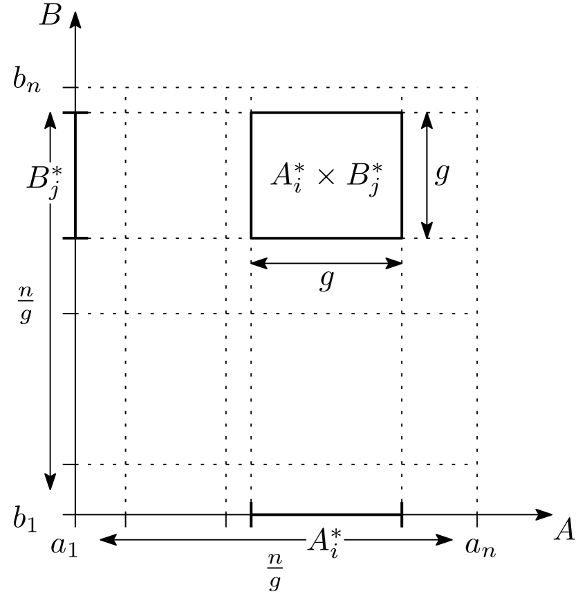
(a) Partitioning $A$ and $B$.

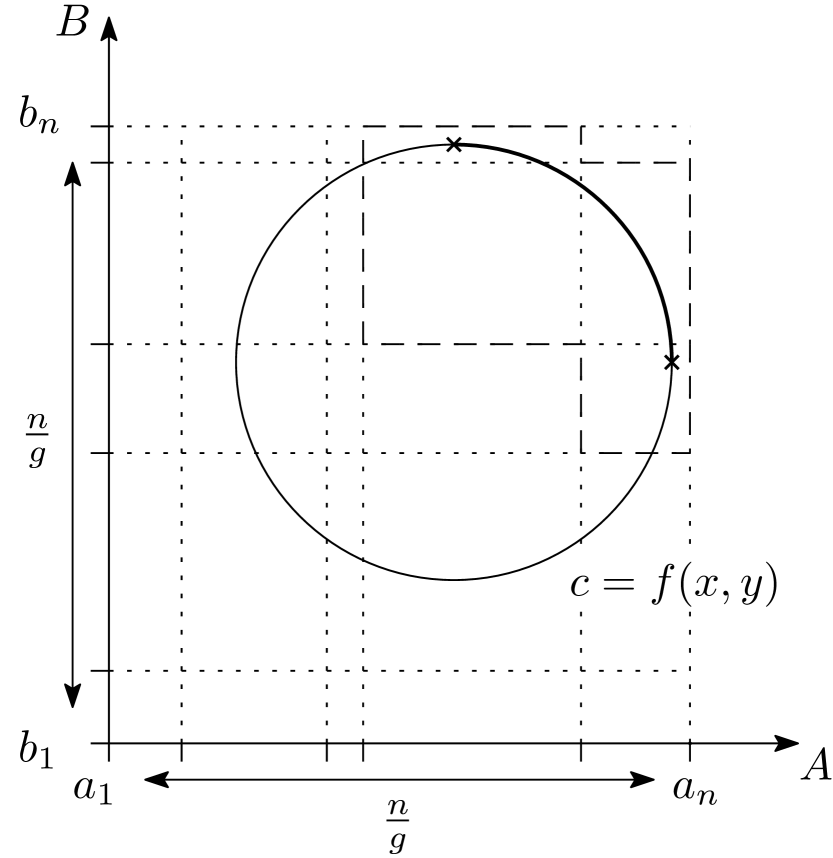
(b) An $xy$-monotone arc of $c=f(x,y)$ intersects a staircase of at most $2\frac{n}{g}-1$ cells in the grid.

Figure 1. Properties of the $A\times B$ grid.

The following two lemmas result from this construction:

Lemma 2.2.

For a fixed value $c\in C$, the curve $c=f(x,y)$ intersects $O(\frac{n}{g})$ cells. Moreover, those cells can be found in $O(\frac{n}{g})$ time.

Proof 2.3.

Since $f$ has constant degree, the curve $c=f(x,y)$ can be decomposed into a constant number of $xy$-monotone arcs. Split the curve into $x$-monotone pieces, then each $x$-monotone piece into $y$-monotone arcs. The endpoints of the $xy$-monotone arcs are the intersections of $f(x,y)=c$ with its derivatives $f^{\prime}_{x}(x,y)=0$ and $f^{\prime}_{y}(x,y)=0$. By Bézout’s theorem, there are $O({\deg(f)}^{2})$ such intersections and so $O({\deg(f)}^{2})$ $xy$-monotone arcs. Figure 1(b) shows that each such arc intersects at most $2\frac{n}{g}-1$ cells since the cells intersected by a $xy$-monotone arc form a staircase in the grid. This proves the first part of the lemma. To prove the second part, notice that for each connected component of $c=f(x,y)$ intersecting at least one cell of the grid either: (1) it intersects a boundary cell of the grid, or (2) it is a (singular) point or contains vertical and horizontal tangency points. The cells intersected by $c=f(x,y)$ are computed by exploring the grid from $O(\frac{n}{g})$ starting cells. Start with an empty set. Find and add all boundary cells containing a point of the curve. Finding those cells is achieved by solving the Tarski sentence $\exists(x,y)c=f(x,y)\land x\in A_{i}^{*}\land y\in B_{j}^{*}$, for each cell $A_{i}^{*}\times B_{j}^{*}$ on the boundary. This takes $O(\frac{n}{g})$ time. Find and add the cells containing endpoints of $xy$-monotone arcs of $c=f(x,y)$. Finding those cells is achieved by first finding the constant number of vertical and horizontal slabs $A_{i}^{*}\times\mathbb{R}$ and $\mathbb{R}\times B_{j}^{*}$ containing such points:

$$\exists(x,y)c=f(x,y)\land(f^{\prime}_{x}(x,y)=0\lor f^{\prime}_{y}(x,y)=0)\land x\in A_{i}^{*},$$

$$\exists(x,y)c=f(x,y)\land(f^{\prime}_{x}(x,y)=0\lor f^{\prime}_{y}(x,y)=0)\land y\in B_{j}^{*}.$$

This takes $O(\frac{n}{g})$ time. Then for each pair of vertical and horizontal slab containing such a point, check that the cell at the intersection of the slab also contains such a point:

$$\exists(x,y)c=f(x,y)\land(f^{\prime}_{x}(x,y)=0\lor f^{\prime}_{y}(x,y)=0)\land x\in A_{i}^{*}\land y\in B_{j}^{*}.$$

This takes $O(1)$ time. Note that we can always assume the constant-degree polynomials we manipulate are square-free, as making them square-free is trivial [Y76]: since $\mathbb{R}[x]$ and $\mathbb{R}[y]$ are unique factorization domains, let $Q=P/\text{gcd}(P,P^{\prime}_{x};x)$ and $\text{sf}(P)=Q/\text{gcd}(P,P^{\prime}_{y};y)$, where $\text{gcd}(P,Q;z)$ is the greatest common divisor of $P$ and $Q$ when viewed as polynomials in $R[z]$ where $R$ is a unique factorization domain and $\text{sf}(P)$ is the square-free part of $P$. The set now contains, for each component of each type, at least one cell intersected by it. Initialize a list with the elements of the set. While the list is not empty, remove any cell from the list, add each of the eight neighbouring cells to the set and the list, if it contains a point of $c=f(x,y)$ — this can be checked with the same sentences as in the boundary case — and if it is not already in the set. This costs $O(1)$ per cell intersected. The set now contains all cells of the grid intersected by $c=f(x,y)$.

Lemma 2.4.

If the sets $A,B,C$ can be preprocessed in $S_{g}(n)$ time so that, for any given cell $A_{i}^{*}\times B_{j}^{*}$ and any given $c\in C$, testing whether $c\in f(A_{i}\times B_{j})=\{\,f(a,b)\colon\,(a,b)\in A_{i}\times B_{j}\,\}$ can be done in $O(\log g)$ time, then, explicit 3POL can be solved in $S_{g}(n)+O(\frac{n^{2}}{g}\log g)$ time.

Proof 2.5.

We need $S_{g}(n)$ preprocessing time plus the time required to search each of the $n$ numbers $c\in C$ in each of the $O(\frac{n}{g})$ cells intersected by $c=f(x,y)$. Each search costs $O(\log g)$ time. We can compute the cells intersected by $c=f(x,y)$ in $O(\frac{n}{g})$ time by Lemma 2.2.

Remark 2.6.

We do not give a $S_{g}(n)$-time real-RAM algorithm for preprocessing the input, but only a $S_{g}(n)$-depth bounded-degree ADT. In fact, this preprocessing step is the only nonuniform part of Algorithm 2. A real-RAM implementation of this step is given in §3.

(a) The pairs $(a,b),(a^{\prime},b^{\prime})$.

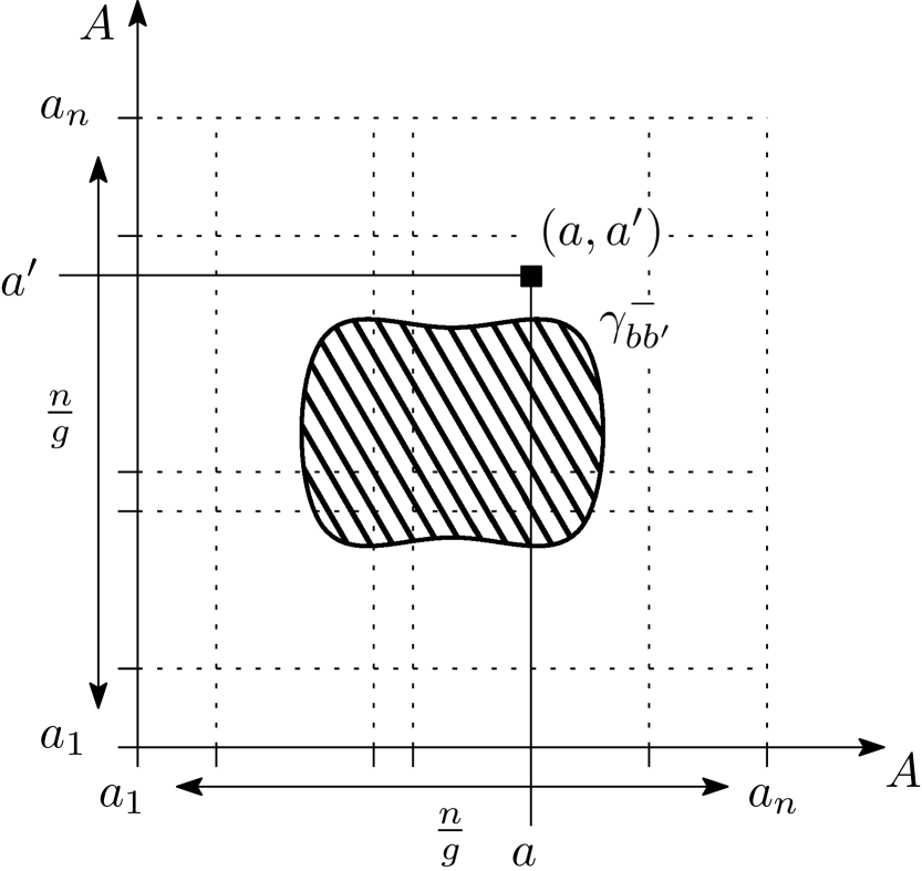
(b) $(a,a^{\prime})\in\gamma^{+}_{b,b^{\prime}}$ implies $f(a,b)>f(a^{\prime},b^{\prime})$.

Figure 2. Generalization of Fredman’s trick (Lemma 2.7).

Preprocessing

All that is left to prove is that $S_{g}(n)$ is subquadratic for some choice of $g$. To achieve this we sort the points inside each cell using Fredman’s trick [F76]. Grønlund and Pettie [GP14] use this trick to sort the sets $A_{i}+B_{j}=\{\,a+b\colon\,(a,b)\in A_{i}\times B_{j}\,\}$ with few comparisons: sort the set $D=(\cup_{i}[A_{i}-A_{i}])\cup(\cup_{j}[B_{j}-B_{j}])$, where $A_{i}-A_{i}=\{\,a-a^{\prime}\colon\,(a,a^{\prime})\in A_{i}\times A_{i}\,\}$ and $B_{j}-B_{j}=\{\,b-b^{\prime}\colon\,(b,b^{\prime})\in B_{j}\times B_{j}\,\}$, using $O(n\log n+|D|)$ comparisons, then testing whether $a+b\leq a^{\prime}+b^{\prime}$ can be done using the free (already computed) comparison $a-a^{\prime}\leq b^{\prime}-b$. We use a generalization of this trick to sort the sets $f(A_{i}\times B_{j})$. For each $B_{j}$, for each pair $(b,b^{\prime})\in B_{j}\times B_{j}$, define the curve $\gamma_{b,b^{\prime}}=\{\,(x,y)\colon\,f(x,b)=f(y,b^{\prime})\,\}.$ Define the sets $\gamma^{0}_{b,b^{\prime}}=\gamma_{b,b^{\prime}},\gamma^{-}_{b,b^{\prime}}=\{\,(x,y)\colon\,f(x,b)<f(y,b^{\prime})\,\},\gamma^{+}_{b,b^{\prime}}=\{\,(x,y)\colon\,f(x,b)>f(y,b^{\prime})\,\}$. The following lemma — illustrated by Figure 2 — follows by definition:

Lemma 2.7.

Given a cell $A_{i}^{*}\times B_{j}^{*}$ and two pairs $(a,b),(a^{\prime},b^{\prime})\in A_{i}\times B_{j}$, deciding whether $f(a,b)<f(a^{\prime},b^{\prime})$ (respectively $f(a,b)=f(a^{\prime},b^{\prime})$ and $f(a,b)>f(a^{\prime},b^{\prime})$) amounts to deciding whether the point $(a,a^{\prime})$ is contained in $\gamma^{-}_{b,b^{\prime}}$ (respectively $\gamma^{0}_{b,b^{\prime}}$ and $\gamma^{+}_{b,b^{\prime}}$).

There are $N\coloneqq\frac{n}{g}\cdot g^{2}=ng$ pairs $(a,a^{\prime})\in\cup_{i}[A_{i}\times A_{i}]$ and there are $N$ pairs $(b,b^{\prime})\in\cup_{j}[B_{j}\times B_{j}]$. Sorting the $f(A_{i}\times B_{j})$ for all $(A_{i},B_{j})$ amounts to solving the following problem:

Problem 2.8 (Polynomial Batch Range Searching).

Given $N$ points and $N$ polynomial curves in $\mathbb{R}^{2}$, locate each point with respect to each curve.

We can now refine the description of step 2 in Algorithm 2

Algorithm 2 (Sorting the $f(A_{i}\times B_{j})$ with a nonuniform algorithm).

input:

$A=\{\,a_{1}<a_{2}<\cdots<a_{n}\,\},B=\{\,b_{1}<b_{2}<\cdots<b_{n}\,\}\subset\mathbb{R}$

output:

The sets $f(A_{i}\times B_{j})$, sorted.

2.1.:

Locate each point $(a,a^{\prime})\in\cup_{i}[A_{i}\times A_{i}]$ w.r.t. each curve $\gamma_{b,b^{\prime}},(b,b^{\prime})\in\cup_{j}[B_{j}\times B_{j}]$.

2.2.:

Sort the sets $f(A_{i}\times B_{j})$ using the information retrieved in step 2.1.

Note that this algorithm is nonuniform: step 2.2 costs at least quadratic time in the real-RAM model, however, this step does not need to query the input at all, as all the information needed to sort is retrieved during step 2.1. Step 2.2 incurs no cost in our nonuniform model.

To implement step 2.1, we use a modified version of the $N^{\frac{4}{3}}2^{O(\log^{*}N)}$ algorithm of Matoušek [Ma93] for Hopcroft’s problem. In Appendix LABEL:sec:algo:point-curves-location, we prove the following upper bound:

Lemma 2.9.

Polynomial Batch Range Searching can be solved in $O(N^{\frac{4}{3}+\varepsilon})$ time in the real-RAM model when the input curves are the $\gamma_{b,b^{\prime}}$.

Analysis

Combining Lemma 2.4 and Lemma 2.9 yields a $O({(ng)}^{4/3+\varepsilon}+n^{2}g^{-1}\log g)$-depth bounded-degree ADT for 3POL. By optimizing over $g$, we get $g=\Theta(n^{2/7-\varepsilon})$, and the previous expression simplifies to $O(n^{12/7+\varepsilon})$, proving Theorem 2.1.

3. Uniform algorithm for explicit 3POL

We now build on the first algorithm and prove the following:

Theorem 3.1.

Explicit 3POL can be solved in $O(n^{2}{(\log\log n)}^{\frac{3}{2}}/{(\log n)}^{\frac{1}{2}})$ time.

We generalize again Grønlund and Pettie [GP14]. The algorithm we present is derived from the first subquadratic algorithm in their paper.

Idea

We want the implementation of step 2 in Algorithm 2 to be uniform, because then, the whole algorithm is. We use the same partitioning scheme as before except we choose $g$ to be much smaller. This allows to store all permutations on $g^{2}$ items in a lookup table, where $g$ is chosen small enough to make the size of the lookup table $\Theta(n^{\varepsilon})$. The preprocessing part of the previous algorithm is replaced by $g^{2}!$ calls to an algorithm that determines for which cells a given permutation gives the correct sorted order. This preprocessing step stores a constant-size pointer from each cell to the corresponding permutation in the lookup table. Search can now be done efficiently: when searching a value $c$ in $f(A_{i}\times B_{j})$, retrieve the corresponding permutation on $g^{2}$ items from the lookup table, then perform binary search on the sorted order defined by that permutation. The sketch of the algorithm is exactly Algorithm 2. The only differences with respect to §2 are the choice of $g$ and the implementation of step 2.

$A\times B$ grid partitioning

We use the same partitioning scheme as before, hence Lemma 2.2 and Lemma 2.4 hold. We just need to find a replacement for Lemma 2.9.

Preprocessing

For their simple subquadratic 3SUM algorithm, Grønlund and Pettie [GP14] explain that for a permutation to give the correct sorted order for a cell, that permutation must define a certificate — a set of inequalities — that the cell must verify. They cleverly note — using Fredman’s Trick [F76] as in Chan [Cha08] and Bremner et al. [BCDEHILPT14] — that the verification of a single certificate by all cells amounts to solving a red/blue point dominance reporting problem. We generalize their method. For each permutation $\pi\colon\,[g^{2}]\to{[g]}^{2}$, where $\pi=(\pi_{r},\pi_{c})$ is decomposed into row and column functions $\pi_{r},\pi_{c}\colon\,[g^{2}]\to[g]$, we enumerate all cells $A_{i}^{*}\times B_{j}^{*}$ for which the following certificate holds:

$$f(a_{i,\pi_{r}(1)},b_{j,\pi_{c}(1)})\leq f(a_{i,\pi_{r}(2)},b_{j,\pi_{c}(2)})\leq\cdots\leq f(a_{i,\pi_{r}(g^{2})},b_{j,\pi_{c}(g^{2})}).$$