An Exact Redatuming Procedure for the Inverse Boundary Value Problem for the Wave Equation

Abstract

Redatuming is a data processing technique to transform measurements recorded in one acquisition geometry to an analogous data set corresponding to another acquisition geometry, for which there are no recorded measurements. We consider a redatuming problem for a wave equation on a bounded domain, or on a manifold with boundary, and model data acquisition by a restriction of the associated Neumann-to-Dirichlet map. This map models measurements with sources and receivers on an open subset $\Gamma$ contained in the boundary of the manifold. We model the wavespeed by a Riemannian metric, and suppose that the metric is known in some coordinates in a neighborhood of $\Gamma$. Our goal is to move sources and receivers into this known near boundary region. We formulate redatuming as a collection of unique continuation problems, and provide a two step procedure to solve the redatuming problem. We investigate the stability of the first step in this procedure, showing that it enjoys conditional Hölder stability under suitable geometric hypotheses. In addition, we provide computational experiments that demonstrate our redatuming procedure.

35R30, 35L05

1 Introduction

We consider an exact redatuming procedure for the inverse boundary value problem for the wave equation. We let $M$ be a bounded domain in $\mathbb{R}^{n}$, or more generally a smooth manifold with boundary, and assume that its boundary $\partial M$ is smooth. Then, we consider the wave equation

(1) $$(\partial_{t}^{2}-\Delta_{g})u(t,x) =0, (t,x)\in(0,\infty)\times M,$$

$$\partial_{\nu}u(t,x) =f(t,x), (t,x)\in(0,\infty)\times\partial M,$$

$$u(0,x)=\partial_{t}u(0,x) =0, x\in M,$$

where $\Delta_{g}$ denotes the Laplace-Beltrami operator for a metric tensor $g$ on $M$. Let us remark that, in the case of a domain, this Riemannian formulation allows us to consider both the cases of isotropic and elliptically anisotropic wavespeeds. We suppose that the metric $g$ is known, for some fixed $r>0$ and in some fixed coordinates, in the domain of influence $M(\Gamma,r)$, defined by:

(2) $$M(\Gamma,r):=\{x\in M:d(x,\Gamma)\leq r\}.$$

Outside of this set, the metric will be assumed to be unknown. We suppose that $g$ is smooth in $M(\Gamma,r)$, but allow for $g$ to possess singularities of conormal type in the complement of this set.

The term redatuming comes from the seismic literature, where it is used to refer to procedures to synthesize measurements for another set where data has not been recorded (see e.g. [19]). In the present setting, we suppose that data has been collected on an open subset $\Gamma\subset\partial M$ in the form of the Neumann-to-Dirichlet map (N-to-D map). Specifically, we suppose that for a fixed fixed time $T>0$, we have the N-to-D map $\Lambda_{\Gamma}^{2T}$, defined by:

$$\Lambda_{\Gamma}^{2T}f=u^{f}|_{(0,2T)\times\Gamma},\quad f\in C_{0}^{\infty}((0,2T)\times\Gamma)$$

where $u^{f}$ is the solution of (1). Let $\Omega\subset M(\Gamma,r)$ be the set into which we would like to “move” the sources and receivers. To make this precise, let $F$ be an interior source supported in $[0,T/2]\times\Omega$, and let $w^{F}$ solve

(3) $$(\partial_{t}^{2}-\Delta_{g})w(t,x) =F(t,x), (t,x)\in(0,\infty)\times M,$$

$$\partial_{\nu}w(t,x) =0, (t,x)\in(0,\infty)\times\partial M,$$

$$w(0,x)=\partial_{t}w(0,x) =0, x\in M.$$

We define the map:

(4) $$\mathcal{L}:F\mapsto w^{F}|_{[0,T/2]\times\Omega},\qquad\text{for $F\in L^{2}([0,T/2]\times\Omega)$.}$$

Then, redatuming into $\Omega$ can be accomplished by constructing the map $\mathcal{L}$ using the data $\Lambda_{\Gamma}^{2T}$ and $g|_{M(\Gamma,r)}$. Thus the central focus of this paper is the following problem:

• Given $\Lambda_{\Gamma}^{2T}$ and $g|_{M(\Gamma,r)}$, determine the map $\mathcal{L}$.

In Section 3 we develop an algorithm to solve problem (P) constructively.

Our primary motivation for studying the problem (P) stems from the fact that it arises as a step in several variations of the Boundary Control (BC) method, see [3] for the original formulation of the method. In theory, the BC method allows one to reconstruct $(M,g)$ given $\Lambda_{\Gamma}^{2T}$ for $T>\max_{x\in M}d(x,\Gamma)$. This reconstruction is based on a layer stripping argument, for which the first step is to recover $g$ in the semigeodesic coordinates of $\Gamma$. As these coordinates do not cover the whole $M$, we refer to this procedure as the local recovery step. The second step is to solve the redatuming problem (P), and consequently we refer to this step as the redatuming step. Solving Problem (P) allows one to propagate the data $\Lambda_{\Gamma}^{2T}$ into the interior of $M$ and thus enables one to repeat the local recovery step with data in the interior. By alternating between the local recovery and redatuming steps, one can reconstruct the Riemannian structure $(M,g)$ further and further away from $\Gamma$. In particular, one can reconstruct the structure outside the domain where the semigeodesic coordinates of $\Gamma$ are applicable.

Such an alternating iteration has been used in several uniqueness results for inverse boundary value problems [9, 10, 14, 16], however, the iteration is unstable, and it has not been implemented computationally to our knowledge. In order to understand how to regularize the iteration, we need to study the inherent instability of the local recovery and redatuming steps. The present paper considers the redatuming step, that is, the problem (P), while we have previously studied the local recovery step [5].

We divide our redatuming procedure into two steps, which we call moving receivers and sources, respectively. The moving receivers step concerns solving the following time-windowed problem:

• Given $\Lambda_{\Gamma}^{2T}f|_{(T-r,T+r)\times\Gamma}$ for $f\in L^{2}([0,T-r]\times\Gamma)$, determine $u^{f}(T,\cdot)$ in $\Omega$. Here, $g$ is known in $M(\Gamma,r)$.

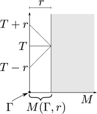
Figure 1: Geometry of the windowed problem (WP). The shaded region indicates where the metric is unknown.

Time-windowing arises naturally in the redatuming problem, and it also allows us to consider the problem (WP) as a unique continuation problem for the wave equation on $(T-r,T+r)\times M(\Gamma,r)$. We illustrate the geometry of (WP) in Figure 1. Let us note that, as $f$ is assumed to be supported on $[0,T-r]\times\overline{\Gamma}$, $u^{f}$ satisfies the homogeneous Neumann boundary condition on $(T-r,T+r)\times\partial M$. In our computational procedure, we will allow $f$ to have support in $[T-r,T]\times\Gamma$. This does not affect the stability properties of the moving receivers step, since if $f\in L^{2}([T-r,T]\times\Gamma)$, then solving (1) in $M$ to obtain $u^{f}(T,\cdot)$ is a classical well-posed problem, when $g$ is known on $M(\Gamma,r)$.

We will show that, after a transposition, the moving sources step reduces to a problem analogous to (WP). For this reason, we develop stability theory only for the moving receivers step.

The problem (WP) is a special case of the following unique continuation problem

• Given Cauchy data $(u,\partial_{\nu}u)$ on $(T-r,T+r)\times\Gamma$, determine $u(T,\cdot)$ near $\Gamma$. Here, $u$ satisfies $\partial_{t}^{2}u-\Delta_{g}u=0$, and $g$ is known in $M(\Gamma,r)$.

Thus, the stability of (WP) can be no less favorable than that of (UC). On the other hand, since problem (WP) considers waves that satisfy a global Neumann boundary condition, while no such boundary conditions are imposed in (UC), it is not immediately evident how the stability of (WP) compares to that of (UC). Nonetheless, we will show that (WP) enjoys the same stability as (UC), and we present sharp stability theory for the problem (WP) in Section 2.

Let us briefly summarize the stability theory. Under suitable conditions, the problem (UC) is known to be conditionally Hölder stable, see e.g. [8, Thm. 3.2.2]. We give a geometric reformulation of this result in terms of convexity of $\Gamma$, and show that conditional Hölder stability is optimal for (UC). Our counterexample establishing the optimality of Hölder type stability works in the case of strictly convex $\Gamma$, and moreover, we show that a refined version of this counterexample also works in the case of the windowed problem (WP). In particular, this shows that the global homogeneous Neumann boundary condition on $(T-r,T+r)\times\partial M$ in (WP) does not improve the stability. This should be contrasted with [1], where unconditional Lipschitz stability is obtained for a problem of the form (WP), with strictly convex $\Gamma$, under the additional assumption that $u^{f}(T,\cdot)$ and $\partial_{t}u^{f}(T,\cdot)$ are supported near $\Gamma$.

Unique continuation problems have been studied from computational point of view, for example, the so-called quasireversibility method has been used to solve (UC) in [13]. In this paper we propose to use the iterative time-reversal control method due to Bingham et. al. [4] to solve (WP). In [4] this method was applied to the coefficient determination problem to find $g$ given $\Lambda_{\Gamma}^{2T}$, however, as explained in Section 3, it can be used to solve (WP) as well. We describe also the moving sources step in Section 3 and give there a complete algorithm solving (P). Finally, we give computational examples in Section 4. To our knowledge, this is the first computational implementation of the iterative time-reversal control method.

2 Stability Theory for the Windowed Problem

In this section, we consider the stability theory for the windowed problem (WP). We begin by recalling the stability theory for the more general problem (UC). We were not able to find all the results in Sections 2.1-3 in the literature, however, the techniques used there are well-known.

2.1 Conditional Hölder stability for UC under convexity conditions

We use ideas from [8, 22] to prove the following conditional Hölder stability estimate:

Lemma 2.1.

Let $T>0$, $x_{0}\in\Gamma$, and suppose that $\Gamma\subset\partial M$ is strictly convex in the sense of the second fundamental form. Then there exist a neighbourhood $U$ of $(0,x_{0})$ in $(-T,T)\times M$, $\kappa\in(0,1)$ and $C>0$ such that for all $u\in H^{2}((-T,T)\times M)$ satisfying $\partial_{t}^{2}u-\Delta_{g}u=0$ it holds that

(5) $$\|u\|_{H^{1}\left(U\right)}\leq C(F+A^{1-\kappa}F^{\kappa}),$$

where $F=\|u\|_{H^{3/2}((-T,T)\times\Gamma)}+\|\partial_{\nu}u\|_{H^{1/2}((-T,T)\times\Gamma)}$ and $A=\|u\|_{H^{1}((-T,T)\times M)}$.

Proof 2.2.

Let $\Gamma^{\prime}\subset\Gamma$ be a coordinate neighbourhood of $x_{0}$, let $s_{0}>0$ be small, and set $\Omega=(-s_{0},s_{0})\times\Gamma^{\prime}$. We will use semigeodesic coordinates $(s,y)\in\Omega$ associated to $\Gamma^{\prime}$. Here a point $x\in M$ near $x_{0}$ has the coordinates $(s,y)$ where $y$ is the closest point to $x$ in $\Gamma^{\prime}$ and $s=d(x,y)$. Furthermore, we choose the coordinates so that $x_{0}=(0,0)$, and extend $g$ smoothly to $\Omega$. All norms, inner products, gradients and Hessians will be taken with respect to the Riemannian structure associated with $g$ on $\Omega$.

Let $Q=(-T_{0},T_{0})\times\Omega$ for some $T_{0}\in(0,T]$. We recall that if a function $\phi$ is strongly pseudo-convex in $\overline{Q}$ with respect to the wave operator $P:=\partial_{t}^{2}-\Delta_{g}$, then, for $v\in C_{0}^{\infty}(Q)$ one has the Carleman estimate [7, Thm. 28.2.3]:

(6) $$\tau\int_{Q}e^{2\tau\phi}(|\partial_{t}v|^{2}+|\nabla v|^{2}+\tau^{2}|v|^{2})dtdx\leq C\int_{Q}e^{2\tau\phi}|Pv|^{2}dtdx,\quad\tau>1.$$

By approximation, this estimate also extends to $v\in H_{0}^{2}(Q)$ .

To obtain a function $\phi$ that is strongly pseudo-convex in $\overline{Q}$ , we follow the approach from [22]. Specifically, we construct a function $\psi$ satisfying:

1. $|\partial_{t}\psi|\neq|\nabla\psi|$ in $Q$,

2. $H_{p}^{2}\psi>0$ on $T^{*}(\overline{\Omega})\setminus 0$ whenever $\psi=p=H_{p}\psi=0$,

where, $H_{p}$ denotes the Hamiltonian flow associated with principal symbol $p$ of $P$. If $\psi$ satisfies (i)-(ii), then the function $\phi:=\exp(\beta\psi)-1$ will be strongly pseudo-convex in $\overline{Q}$, provided that $\beta\gg 1$. Moreover, when $\psi(t,x)=\theta(t)+\rho(x)$, condition (ii) is equivalent to

(7) $$\partial_{t}^{2}\theta+D^{2}\rho(\xi,\xi)>0,\quad\xi\in S_{x}M,\ (t,x)\in Q,$$

holding whenever $\partial_{t}\theta\pm(\xi,\nabla\rho)=0$, see e.g. [22]. Here, we use $S_{x}M$ to denote the unit sphere at $x$.

In order to derive (5) from (6) via a cut-off argument, the function $\psi$ needs to be chosen so that it decays when the distance to the origin $(t,s,y)=(0,0,0)$ grows in the region $s>0$. Let $R,\delta,\mu>0$, and consider the polynomial

$$\psi(t,s,y)=(R-s)^{2}-\delta t^{2}-\mu|y|^{2}-R^{2}.$$

Here, we identify $y$ with its coordinate representation and use $|y|$ to denote the Euclidean length of the coordinate vector for $y$. The function $\psi$ decays as needed when $0<s<R$. Let us show that $R$, $\delta$ and $\mu$ can be chosen so that $\psi$ satisfies (7). Consider first the case $\mu=0$. Then, on the boundary, $s=0$ and this inequality reduces to

$$-\delta+\sigma^{2}+R\operatorname{II}(\eta,\eta)>0,\quad\xi=(\sigma,\eta),$$

where $\operatorname{II}$ denotes the second fundamental form for $\Gamma$. By strict convexity, it holds that $R\operatorname{II}(\eta,\eta)\geq|\eta|^{2}$ for large enough $R>0$. Moreover, $\sigma^{2}+|\eta|^{2}=|\xi|^{2}=1$, and therefore (7) holds if $\delta<1$. The inequality (7) remains valid in a neighbourhood of the origin for small $\mu>0$ by smoothness. To show that (i) holds, we note that $\partial_{t}\psi(0,0)=0$ and $|\nabla\psi(0,0)|\geq 2R$, thus $|\partial_{t}\psi|\neq|\nabla\psi|$ at the origin. Smoothness of $\psi$ implies that this condition also holds in a neighborhood of the origin. Then, we can shrink $Q$ by decreasing $s_{0}$, $T_{0}$, and $\Gamma^{\prime}$, in order to ensure that $\psi$ satisfies (i) and (ii) on $Q$.

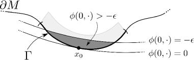
Figure 2: A cartoon illustrating the geometry for Lemma 2.1 at $t=0$. The lightly shaded region represents $Q^{+}\cap\{t=0\}$, while the dark region depicts $U(\epsilon)\cap\{t=0\}$. For this simple case we have taken $\Gamma^{\prime}=\Gamma$.

We write $Q^{+}=Q\cap\{s>0\}$, and use the right inverse of the trace map to get $w\in H^{2}(Q^{+})$ with Cauchy data $(u,\partial_{\nu}u)$ on $(-T,T)\times\Gamma^{\prime}$ satisfying $\|w\|_{H^{2}(Q^{+})}\leq CF$. Then, $v=u-w$ has zero Cauchy data on $(-T,T)\times\Gamma^{\prime}$ and we extend $v$ by zero as a function on $Q$. Then, $f=Pv=-Pw$ satisfies $\left\|f\right\|_{L^{2}(Q^{+})}\leq CF$. We note that $\psi<0$ in $Q^{+}$ so $\phi<0$ there too. Choose $\epsilon>0$ sufficiently small so that the set

$$U(\epsilon)=\{(t,s,y)\in\mathbb{R}^{1+n};\ \phi(t,s,y)\geq-\epsilon,\ s>0\}$$

satisfies $U(\epsilon)\subset Q^{+}$, and choose $\chi\in C_{0}^{\infty}(Q)$ such that $\chi=1$ in $U(\epsilon)$. See Figure 2 for an illustration.

We will apply (6) to $\chi v$. Note that

$$P(\chi v)=\chi Pv+[P,\chi]v=\chi f+[P,\chi]v,$$

where the commutator $[P,\chi]$ is a first-order differential operator that vanishes on the set $U(\epsilon)$. Thus

$$\tau\int_{U(\epsilon/2)}e^{2\tau\phi}\left(|\partial_{t}v|^{2}+|\nabla v|^{2}+\tau^{2}|v|^{2}\right)dtdx$$

$$\quad\leq C\left(\int_{Q^{+}}e^{2\tau\phi}|f|^{2}dtdx+\int_{Q^{+}\setminus U(\epsilon)}e^{2\tau\phi}|[P,\chi]v|^{2}dtdx\right).$$

Using that $\tau>1$, and setting $p=2\left\|\phi\right\|_{L^{\infty}(Q)}+\epsilon$, it holds that

$$\left\|v\right\|_{H^{1}(U(\epsilon/2))}^{2}\leq C\left(e^{\tau p}\left\|f\right\|_{L^{2}(Q^{+})}^{2}+e^{-\tau\epsilon}\left\|v\right\|_{H^{1}(Q^{+})}^{2}\right).$$

Since $v=u+w$ and $\|w\|_{H^{2}(Q^{+})}\leq CF$ we have that $\|v\|_{H^{1}(Q^{+})}\leq C(A+F)$. Recalling that $\|f\|_{L^{2}(Q^{+})}\leq CF$, we find:

$$\left\|v\right\|_{H^{1}(U(\epsilon/2))}^{2}\leq C\left(e^{\tau p}F^{2}+e^{-\tau\epsilon}(A+F)^{2}\right).$$

Choosing $\tau$ as in [8, Thm. 3.2.2], we obtain

$$\left\|v\right\|_{H^{1}(U(\epsilon/2))}\leq CF^{\kappa}(A+F)^{1-\kappa},$$

where $\kappa=\epsilon/(p+\epsilon)$. Then, since $0<1-\kappa<1$, we see that $(A+F)^{1-\kappa}\leq A^{1-\kappa}+F^{1-\kappa}$. Finally, we again use that $v=u+w$ and the bound on $\|w\|_{H^{2}(Q^{+})}$ to conclude:

$$\left\|u\right\|_{H^{1}(U(\epsilon/2))}\leq C(F+A^{1-\kappa}F^{\kappa}).$$

2.2 Convexity is necessary for Hölder stability

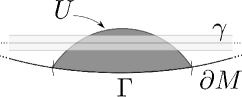
Figure 3: Example where a geodesic $\gamma$ passes through $U$ but fails to intersect $\Gamma$. The dark shaded region is a slice of $U$ at some time $t$, and the light shaded region is the spatial projection of the effective support of a Gaussian beam centered on $\gamma$.

In this section, we demonstrate that a convexity condition must hold between the sets $\Gamma$ and $U$ in order for a Hölder stability estimate of the type (5) to hold. We follow ideas from [21], and show that if there is a bicharacteristic ray that passes over $U$ but does not meet $[-T,T]\times\overline{\Gamma}$, then (5) can not hold.

Let $\gamma$ be a unit speed geodesic on $M$ and consider the corresponding bicharacteristic ray $\beta(t)=(t,\gamma(t))$. We suppose that there exists $t_{0}\in(-T,T)$ for which $(t_{0},\gamma(t_{0}))\in U$ but $\gamma(t)\not\in\overline{\Gamma}$ for all $t\in[-T,T]$. Let us consider a Gaussian beam $u_{\epsilon}$ concentrated on $\gamma$. We refer to [10, 21] for the construction of Gaussian beams, and recall here only that, for $\epsilon>0$, $u_{\epsilon}$ is a family of solutions to the wave equation $\partial_{t}^{2}u_{\epsilon}-\Delta_{g}u_{\epsilon}=0$ on $(-T,T)\times M$ satisfying for any $j\in\mathbb{N}_{0}$ and multi-index $\lambda\in\mathbb{N}_{0}^{n}$

$$|\partial_{t}^{j}\partial_{x}^{\lambda}(u_{\epsilon}(t,x)-\chi(t,x)U_{\epsilon}^{N}(t,x))|\leq C_{j,\lambda,N}\epsilon^{N-(j+|\lambda|+n/4)},\quad t\in(-T,T),\ x\in M.$$

Here, $\chi$ is a smooth function having small support around $\beta$ and satisfying $\chi=1$ near $\beta$, and in local coordinates $(t,z)$, $U_{\epsilon}^{N}$ is a smooth function of the form

$$U_{\epsilon}^{N}(t,z)=\epsilon^{-n/4}\exp\left(i\epsilon^{-1}\Theta(t,z)\right)\sum_{j=0}^{N}\epsilon^{j}a_{j}(t,z),\quad N\in\mathbb{N}.$$

Here, $\Theta$ is a complex valued function whose imaginary part vanishes on $\beta$, and satisfies $\Im\Theta(t,z)\geq\theta(t)|z-\gamma(t)|^{2}$ for some continuous strictly positive function $\theta$. Moreover, the function $a_{0}$ does not vanish on $\beta$.

First we discuss how the right hand side of (5) behaves with respect to the family $u_{\epsilon}$. We define, for an integer $r>0$ and each $\epsilon>0$, the quantities,

$$A_{\epsilon}:=\|u_{\epsilon}\|_{H^{r}([-T,T]\times M)},\quad F_{\epsilon}:=\|u_{\epsilon}\|_{H^{r}([-T,T]\times\Gamma)}+\|\partial_{\nu}u_{\epsilon}\|_{H^{r-1}([-T,T]\times\Gamma)},$$

and investigate how they behave as $\epsilon\rightarrow 0$. Since $\beta$ does not intersect $[-T,T]\times\overline{\Gamma}$, we can choose $\chi$ so that it vanishes on $[-T,T]\times\Gamma$. Then,

$$|\partial_{t}^{j}\partial_{x}^{\lambda}u_{\epsilon}(t,x)|\leq C_{j,\lambda,N}\epsilon^{N-(j+|\lambda|+n/4)},\quad\text{for $(t,x)\in[-T,T]\times\Gamma$}.$$

Consequently, for any $r\in\mathbb{N}$, it holds that $F_{\epsilon}\leq C_{r,N}\epsilon^{N-(r+n/4)}$. Now, let us consider the quantity $A_{\epsilon}$. We have $\left\|U_{\epsilon}^{N}\right\|_{H^{r}([-T,T]\times M)}\leq C_{r,N}\epsilon^{-r-n/4}$, and therefore also $A_{\epsilon}\leq C_{r,N}\epsilon^{-r-n/4}$. Thus, for any fixed $0<\kappa<1$, there exists a constant $C_{r,N}>0$ such that

$$F_{\epsilon}+A_{\epsilon}^{1-\kappa}F_{\epsilon}^{\kappa}\leq C_{r,N}\left(\epsilon^{N-(r+n/4)}+\epsilon^{\kappa N-(r+n/4)}\right).$$

Finally, we choose $N$ sufficiently large such that $\kappa N>r+n/4$, and conclude that

(8) $$F_{\epsilon}+A_{\epsilon}^{1-\kappa}F_{\epsilon}^{\kappa}\rightarrow 0\quad\text{as $\epsilon\rightarrow 0$.}$$

We now consider how the left-hand side of (5) behaves with respect to the family $u_{\epsilon}$. In view of (8), it remains to show that $\|u_{\epsilon}\|_{H^{r}(U)}$ stays positive as $\epsilon\rightarrow 0$. Since $\|u_{\epsilon}\|_{H^{r}(U)}\geq\|u_{\epsilon}\|_{L^{2}(U)}$, we can consider only the $L^{2}$ norm. Let $B$ be a ball containing the point $\gamma(t_{0})$ and satisfying $\{t_{0}\}\times B\subset U$. On [10, p. 176], it is shown that $\lim_{\epsilon\rightarrow 0}\|u_{\epsilon}(t,\cdot)\|_{L^{2}(B)}=a(t)$, where $a$ is a continuous strictly positive function. Thus for small $\delta>0$ it holds that $\lim_{\epsilon\rightarrow 0}\|u_{\epsilon}\|_{L^{2}([-\delta,\delta]\times B)}>0$. This concludes the proof, showing that if there is a bicharacteristic ray passing over $U$ that does not meet $[-T,T]\times\overline{\Gamma}$, then (5) cannot hold.

2.3 A counterexample to Lipschitz stability for UC

In this section, we give a counterexample showing that (5) cannot hold with $\kappa=1$. This example is a variation of the classical counterexample by Hadamard [6, p. 33], adapted to a strictly convex setting.

Let us consider a case where $M$ is contained in the half disk

$$\{re^{i\theta}\in\mathbb{C};\ r\in(0,1],\ |\theta|<\pi/2\}.$$

We assume that $M$ is equipped with the Euclidean metric and suppose that $\Gamma\subset\partial M$ is of the form $\Gamma=\{e^{i\theta}\in\mathbb{C};\ |\theta|<\theta_{0}\}$, for some $\theta_{0}\in(0,\pi/2)$.

We consider a family of stationary waves in $M$. For $n\in\mathbb{N}$, we define

$$\phi_{n}(re^{i\theta}):=r^{-n}e^{in\theta}.$$

Then, we recall that in polar coordinates $(r,\theta)\mapsto re^{i\theta}$ the Laplacian has the form

$$\Delta=\partial_{r}^{2}+r^{-1}\partial_{r}+r^{-2}\partial_{\theta}^{2}.$$

Using this formula, it is straightforward to check that the $\phi_{n}$ are harmonic in $M$ (note that $0\not\in M$). Letting $u_{n}(t,x)=\phi_{n}(x)$, it is immediate that $(\partial_{t}^{2}-\Delta)u_{n}=0$ on $\mathbb{R}\times M$.

Next, we observe that $\phi_{n}(1,\theta)=e^{in\theta}$ and $\partial_{\nu}\phi_{n}(1,\theta)=ine^{in\theta}$. Thus,

$$\|(\phi_{n},\partial_{\nu}\phi_{n})\|_{H^{k}(\Gamma)\times H^{k-1}(\Gamma)}\leq\|\phi_{n}\|_{H^{k}(\Gamma)}+n\|\phi_{n}\|_{H^{k-1}(\Gamma)}\sim n^{k}.$$

Then, we let $\epsilon,\theta_{1},s>0$ be small and define the sets $\Omega=(1-\epsilon,1)\times(-\theta_{1},\theta_{1})$ and $U=(T-s,T+s)\times\Omega$. We note that, if $\theta_{1}\leq\theta_{0}$ and $\epsilon$ is sufficiently small, then $\Omega\subset M$. Letting $q=1-\epsilon$, we observe that

$$\left\|\phi_{n}\right\|_{L^{2}(\Omega)}^{2}=\int_{q}^{1}r^{-2n}rdr\int_{-\theta_{1}}^{\theta_{1}}|e^{in\theta}|^{2}d\theta\sim\frac{q^{-2(n-1)}}{n-1}$$

for large $n>0$. Thus, a Lipschitz stability estimate of the form

$$\left\|u\right\|_{H^{k}(U)}\leq C\left\|(u,\partial_{\nu}u)\right\|_{H^{k}\times H^{k-1}((T-s,T+s)\times\Gamma)}$$

leads to a contradiction when we take $u=u_{n}$. To see this, we first note that the left-hand side is bounded below by $Cq^{-(n-1)}/\sqrt{n-1}$, where $C$ is independent of $n$. This holds because $\|u_{n}\|_{L^{2}(U)}=2s\|\phi_{n}\|_{L^{2}(\Omega)}$. On the other hand, the right-hand side of this inequality is comparable to $n^{k}$. Thus, we get the contradiction that

$$q^{-(n-1)}\lesssim n^{k}\sqrt{n-1}$$

for large $n$.

2.4 A counterexample to Lipschitz stability for WP

In this section, we construct a counterexample to Lipschitz type stability for the problem (WP) in the strictly convex boundary setting. Our construction is based on finding a family of Neumann sources $\{f_{n}\}$ producing a family of waves $\{u^{f_{n}}\}$ solving (1) that exhibit similar stability properties to the waves considered in Section 2.3. The waves $u^{f_{n}}$ will then satisfy the hypotheses of (WP), and show that Lipschitz type stability does not hold for (WP). We carry out our construction in two steps. First, for some $\epsilon>0$, we find waves $u_{n}$ with vanishing Neumann traces that behave like the waves from Section 2.3 on $t\in[T-\epsilon,T+\epsilon]$. Then, we use exact controllability to obtain Neumann sources $f_{n}\in L^{2}([0,T-\epsilon]\times\Gamma)$ that reproduce these waves, in the sense that $u^{f_{n}}(t,\cdot)=u_{n}(t,\cdot)$ for $t\geq T-\epsilon$.

We consider the case where $M$ is the unit disk equipped with the Euclidean metric, and $\Gamma=(-\theta_{0},\theta_{0})$ for some $\theta_{0}\in(\pi/2,\pi)$ in polar coordinates. Let $0<\epsilon<T$ and $\Omega\subset M$ a neighborhood of $M(\Gamma,\epsilon)$, and select $\epsilon$ and $\Omega$ sufficiently small that $(0,0)\not\in\overline{\Omega}$. We will make use of a fixed cut-off function $\chi\in C^{\infty}([0,2T]\times M)$ which we choose to have the form $\chi(t,x)=\chi_{t}(t)\chi_{x}(x)$ with $\chi_{t}\in C^{\infty}([0,2T])$ and $\chi_{x}\in C^{\infty}(M)$. In particular, we choose $\chi_{t}$ so that it satisfies $\chi_{t}=1$ on a neighborhood of $[T-\epsilon,2T]$ and $\chi_{t}=0$ on a neighborhood of $[0,T-2\epsilon]$. Also, we choose $\chi_{x}$ to satisfy $\chi_{x}\equiv 1$ on $M(\Gamma,\epsilon)$ and $\chi_{x}\equiv 0$ on $M\setminus\Omega$.

Let $\phi$ be any harmonic function in $\Omega$. Using $\phi$, we define $w$ to be the solution to:

$$(\partial_{t}^{2}-\Delta)w(t,x) =0, (t,x)\in(0,2T)\times M,$$

$$\partial_{\nu}w(t,x) =\partial_{\nu}(\chi(t,x)\phi(x)), (t,x)\in(0,2T)\times\partial M,$$

$$w(T,x)=\chi_{x}\phi,\quad\partial_{t}w(T,x) =0, x\in M,$$

and, let $v$ solve

$$(\partial_{t}^{2}-\Delta)v(t,x) =0, (t,x)\in(0,2T)\times M,$$

$$\partial_{\nu}v(t,x) =\partial_{\nu}(\chi(t,x)\phi(x)), (t,x)\in(0,2T)\times\partial M,$$

$$v(T-2\epsilon,x)=\partial_{t}v(T-2\epsilon,x) =0, x\in M.$$

We define $u=w-v$ and study the properties of $u$ in terms of $w,v$ and $\phi$. Let us observe that $\partial_{\nu}u=0$ on $(0,2T)\times\partial M$, since $\partial_{\nu}w$ and $\partial_{\nu}v$ coincide there.

To begin our analysis of $u$, we show that $w(t,x)=\phi(x)$ for $(t,x)\in K$, where

$$K=\left\{(t,x)\in[T-\epsilon,T+\epsilon]\times M(\Gamma,\epsilon)~{}:~{}d(x,M\setminus M(\Gamma,\epsilon))>\left|t-T\right|\right\}.$$

In order to show that $w=\phi$ on $K$, let us abuse notation and identify $\phi$ with its constant extension in time. Then, we note that $\phi$ is harmonic in $\Omega$ and constant in time, thus, $(\partial_{t}^{2}-\Delta)\phi(t,x)=(\partial_{t}^{2}-\Delta)w(t,x)=0$ on $(T-\epsilon,T+\epsilon)\times\Omega$. Next, we note that $w(T,\cdot)=\phi$ and $\partial_{t}w(T,\cdot)=\partial_{t}\phi=0$ in $M(\Gamma,\epsilon)$. Finally, we observe that $\partial_{\nu}w=\partial_{\nu}\phi$ on $[T-\epsilon,T+\epsilon]\times(\partial M\cap M(\Gamma,\epsilon))$, since $\chi=1$ there. Thus, finite speed of propagation for (1) implies that $w$ and $\phi$ coincide in $K$.

We define $\Sigma=[T-\epsilon,T+\epsilon]\times\Gamma$ and $\Sigma^{\prime}=[T-2\epsilon,T+2\epsilon]\times\partial M$. Then, for a set $U\subset[T-\epsilon,T+\epsilon]\times M$, we investigate how the size of $u$ on $U$ compares to the size of $(u,\partial_{\nu}u)$ on $\Sigma$. To that end, we note that $\partial_{\nu}u=0$ on $\Sigma$ and observe that

$$\|(u,\partial_{\nu}u)\|_{H^{k}(\Sigma)\times H^{k-1}(\Sigma)}=\|u\|_{H^{k}(\Sigma)}\leq\|w\|_{H^{k}(\Sigma)}+\|v\|_{H^{k}(\Sigma)}.$$

We will bound the norms on the right in terms of norms of $\phi$. First, we bound the $H^{k}$ norm of $v$. Since $\chi_{t}$ is identically zero on a neighborhood of $T-2\epsilon$, $\partial_{\nu}v=\partial_{\nu}(\chi\phi)$ vanishes identically on a neighborhood of $\{T-2\epsilon\}\times\partial M$. Because $v(T-2\epsilon,\cdot)=\partial_{t}v(T-2\epsilon,\cdot)=0$, we see that $v$ satisfies compatibility conditions to all orders at $t=T-2\epsilon$. Appealing to standard estimates for the wave equation and trace theorems, we can then show that

$$\|v\|_{H^{k}(\Sigma^{\prime})}\lesssim\|\partial_{\nu}v\|_{H^{\ell}(\Sigma^{\prime})},$$

where $\ell>k$ (in particular $\ell=2k+1$ works). Combining this with the previous estimate and using that $\partial_{\nu}v=\partial_{\nu}w$ on $\Sigma^{\prime}$ yields:

$$\|(u,\partial_{\nu}u)\|_{H^{k}(\Sigma)\times H^{k-1}(\Sigma)}\lesssim\|w\|_{H^{k}(\Sigma)}+\|\partial_{\nu}w\|_{H^{\ell}(\Sigma^{\prime})}.$$

Then, since $\partial_{\nu}w=\partial_{\nu}(\chi\phi)$, $w=\phi$ on $K$, and both $\Sigma\subset K$ and $\Sigma\subset\Sigma^{\prime}$ we conclude:

$$\|(u,\partial_{\nu}u)\|_{H^{k}(\Sigma)\times H^{k-1}(\Sigma)}\lesssim\|\phi\|_{H^{k}(\Sigma^{\prime})}+\|\partial_{\nu}\phi\|_{H^{\ell}(\Sigma^{\prime})}.$$

Next, we let $q=1-\frac{\epsilon}{2}$ and note that $0<q<1$. We consider the set

$$U:=\left\{(t,r,\theta)~{}:~{}T-\frac{\epsilon}{2}<t<T+\frac{\epsilon}{2},~{}~{}q<r<1,~{}~{}\theta\in\Gamma\right\}.$$

Observe that $U\subset K$, so $w=\phi$ on $U$. Again, using standard estimates for the wave equation and that $\partial_{\nu}v=\partial_{\nu}(\chi\phi)$ on $\Sigma^{\prime}$, we can show that

$$\|v\|_{H^{k}(U)}\lesssim\|\partial_{\nu}v\|_{H^{2k}(\Sigma^{\prime})}\lesssim\|\partial_{\nu}\phi\|_{H^{2k}(\Sigma^{\prime})}.$$

Whereas, $w=\phi$ on $U$, so $\|w\|_{H^{k}(U)}=\|\phi\|_{H^{k}(U)}$.

Let us now take $\phi=\phi_{n}$ from the preceding section, and note that $\phi_{n}$ is harmonic in $\Omega$. We let $w_{n},v_{n}$ and $u_{n}$ denote the waves associated with $\phi_{n}$ as constructed above. Then, the estimates given in Section 2.3 imply that, for any $j\in\mathbb{N}$, $\|\phi_{n}\|_{H^{j}(\Sigma^{\prime})}\sim n^{j}$ and $\|\partial_{\nu}\phi_{n}\|_{H^{j}(\Sigma^{\prime})}\sim n^{j+1}$, while $\|\phi_{n}\|_{H^{j}(U)}\geq\|\phi_{n}\|_{L^{2}(U)}\gtrsim q^{-(n-1)}/\sqrt{n-1}$. So,

$$\|u_{n}\|_{H^{k}(U)}=\|w_{n}-v_{n}\|_{H^{k}(U)}\gtrsim\left|\|\phi_{n}\|_{H^{k}(U)}-\|\partial_{\nu}\phi_{n}\|_{H^{2k}(\Sigma^{\prime})}\right|\gtrsim q^{-(n-1)}/\sqrt{n-1}.$$

On the other hand,

$$\|(u_{n},\partial_{\nu}u_{n})\|_{H^{k}(\Sigma)\times H^{k-1}(\Sigma)}\lesssim\|\phi_{n}\|_{H^{k}(\Sigma^{\prime})}+\|\partial_{\nu}\phi_{n}\|_{H^{\ell}(\Sigma^{\prime})}\lesssim n^{k}+n^{\ell+1}.$$

Thus, a Lipschitz stability estimate of the form $\|u\|_{H^{k}(U)}\leq C\|(u,\partial_{\nu}u)\|_{H^{k}(\Sigma)\times H^{k-1}(\Sigma)}$ leads to the contradiction that for all $n$,

$$q^{-(n-1)}\lesssim(n^{k}+n^{\ell+1})\sqrt{n-1}.$$

We now show that, if $\tau:=T-\epsilon$ is sufficiently large, there exists a Neumann source $f_{n}\in L^{2}([0,T-\epsilon]\times\Gamma)$ for which $u^{f_{n}}=u_{n}$ on $[T-\epsilon,T+\epsilon]\times M$. To see this, we first recall that $M$ is the unit disk equipped with the Euclidean metric and that $\Gamma$ contains a neighborhood of the half-circle $\theta\in(-\pi/2,\pi/2)$. This setting is considered on p. 1030 of [2], where it is noted that if $\tau>6$, then any bicharacteristic ray beginning above a point $x\in M$ will pass over $[0,\tau]\times\Gamma$ in a non-diffractive point. Thus by choosing $T$ large enough that $\tau=T-\epsilon>6$, the hypotheses of [2, Th. 4.9] for exactly controlling $M$ from $[0,\tau]\times\Gamma$ will be satisfied. Specifically, the map $f\mapsto(u^{f}(\tau,\cdot),\partial_{t}u^{f}(\tau,\cdot))$ taking $L^{2}([0,\tau]\times\Gamma)\rightarrow H^{1}(M)\times L^{2}(M)$ is surjective (see [2, ex. 2], p. 1059). It is straightforward to check that $(u_{n}(T-\epsilon,\cdot),\partial_{t}u_{n}(T-\epsilon,\cdot))\in H^{1}(M)\times L^{2}(M)$, thus there exists a source $f_{n}\in L^{2}([0,T-\epsilon]\times\Gamma)$ for which $(u^{f_{n}}(T-\epsilon,\cdot),\partial_{t}u^{f_{n}}(T-\epsilon,\cdot))=(u_{n}(T-\epsilon,\cdot),\partial_{t}u_{n}(T-\epsilon,\cdot))$. Finally, we note that the Cauchy data of $u^{f_{n}}$ and $u_{n}$ agree at $t=T-\epsilon$, and the Neumann traces of both $u^{f_{n}}$ and $u_{n}$ vanish on $[T-\epsilon,T+\epsilon]\times\partial M$. Hence, uniqueness for solutions to (1) implies that $u^{f_{n}}|_{[T-\epsilon,T+\epsilon]\times M}=u_{n}|_{[T-\epsilon,T+\epsilon]\times M}$.

To conclude, we have constructed a family of waves $\{u^{f_{n}}\}$ that satisfy the hypotheses of (WP). Because these waves coincide with the waves in the family $\{u_{n}\}$ on both $U$ and $\Sigma$, we see that a Lipschitz type stability estimate cannot hold for (WP).

3 Redatuming

In this section, we present our redatuming procedure, which gives a constructive solution to (P). We begin in subsection 3.1 by briefly reviewing concepts from the iterative time reversal control method [4]. As discussed in the introduction, our approach to redatuming is accomplished in two steps: subsection 3.2 is devoted to moving receivers, while subsection 3.3 is devoted to moving sources.

3.1 Notation and techniques

The Riemannian Volume measure on $M$ is denoted by $dV$, and $dS$ will denote the associated surface measure on $\partial M$. When we evaluate $L^{2}$ inner products, the corresponding integrals will be evaluated with respect to these measures.

We define the control map, which is defined for $f\in L^{2}([0,T]\times\Gamma)$, by,

(9) $$W^{T}f:=u^{f}(T,\cdot).$$

We recall that $W^{T}$ is bounded,

(10) $$W^{T}:L^{2}([0,T]\times\Gamma)\rightarrow L^{2}(M),$$

which follows from [15]. Now we form the connecting operator,

(11) $$K^{T}:=(W^{T})^{*}W^{T}.$$

The operator $K^{T}$ derives its name from the fact that it connects inner-products between waves in the interior to measurements made on the boundary. That is, for $f,h\in L^{2}([0,T]\times\Gamma)$,

(12) $$\langle u^{f}(T,\cdot),u^{h}(T,\cdot)\rangle_{L^{2}(M)}=\langle W^{T}f,W^{T}h\rangle_{L^{2}(M)}=\langle K^{T}f,h\rangle_{L^{2}([0,T]\times\Gamma)}.$$

An essential fact about $K^{T}$ is that it can be obtained by processing the boundary data, $\Lambda_{\Gamma}^{2T}$. Specifically, one can construct $K^{T}$ via the Blagoveščenskiĭ identity, which we use in a form analogous to the expression found in [20],

(13) $$K^{T}=J^{T}\Lambda^{2T}_{\Gamma}\Theta^{T}-R^{T}\Lambda^{T}_{\Gamma}R^{T}J^{T}\Theta^{T}.$$

Here, the operators $R^{T}$, $J^{T}$, and $\Theta^{T}$ are defined as follows: the time reversal operator, $R^{T}:L^{2}([0,T]\times\Gamma)\rightarrow L^{2}([0,T]\times\Gamma)$, is defined by

(14) $$R^{T}f(t,\cdot)=f(T-t,\cdot),\qquad\text{ for $0<t<T$ },$$

the time filtering operator, $J^{T}:L^{2}([0,2T]\times\Gamma)\rightarrow L^{2}([0,T]\times\Gamma)$, is given by,

(15) $$J^{T}f(t,\cdot)=\frac{1}{2}\int_{t}^{2T-t}f(s,\cdot)\,ds,\qquad\text{ for $0<t<T$},$$

and the zero extension operator, $\Theta^{T}:L^{2}([0,T]\times\Gamma)\rightarrow L^{2}([0,2T]\times\Gamma)$, is given by,

(16) $$\Theta^{T}f(t,\cdot)=\left\{\begin{array}[]{ll}f(t,\cdot)&0\leq t\leq T\\ 0&T<t\leq 2T.\\ \end{array}\right.$$

In addition, we will use the restriction, $\rho^{T}:L^{2}([0,2T]\times\Gamma)\rightarrow L^{2}([0,T]\times\Gamma)$, given by $\rho^{T}f=f|_{[0,T]\times\Gamma}$. We will also use, for $r\in[0,T]$, the family of orthogonal projections $P_{r}^{T}:L^{2}([0,T]\times\Gamma)\rightarrow L^{2}([T-r,T]\times\Gamma)$, which too are obtained by restriction. Lastly, for $s>0$, we will use time delay operators, given by

(17) $$Z_{s}\phi(t,\cdot):=\left\{\begin{array}[]{cl}0&\text{for $t\in[0,s]$}\\ \phi(t-s,\cdot)&\text{for $t>s$}.\end{array}\right.$$

We will need analogous operators defined on spaces of the form $L^{2}([0,S]\times A)$, where $A\subset\overline{M}$ and $S>0$. For those operators, we use similar notation. For instance, we will also write $R^{S}$ to denote the time-reversal operator on $L^{2}([0,S]\times A)$. We note that, in all cases, our notation will only indicate the appropriate final time $S$, since all four operators $R,J,\Theta,\rho$ act essentially in the temporal domain. We do not indicate the spatial domain in our notation since it will be evident from context.

Finally, in some longer equations, we will suppress the spatial dependence of functions in our notation. For example, let $F:[0,T]\times M\rightarrow\mathbb{R}$ and $t\in\mathbb{R}$. Then, we will occasionally write $F(t)$ to denote $F(t,\cdot)$.

3.2 Moving Receivers

In this section, we will construct the map $L$,

(18) $$L:f\mapsto u^{f}|_{[0,T]\times M(\Gamma,r)},\quad\text{for $f\in L^{2}([0,T]\times\Gamma)$.}$$

We refer to the procedure for constructing $L$ as moving receivers, since evaluating $L$ is tantamount to extrapolating receivers into $M(\Gamma,r)$. Moving receivers is accomplished through Algorithm 1, and we demonstrate the correctness of this algorithm via Lemma 3.1. We note that Lemma 3.1 is essentially demonstrated in [4, Lemma 7]. However, we repeat the proof here, since it is constructive and forms the basis for Algorithm 1.

  for $f\in C_{0}^{\infty}([0,T]\times\Gamma)$ :

     for all $0<t<T$ :

        for all $0<\alpha$ :

           Let : $h=h_{\alpha,t}$ denote the solution to

$$P_{r}^{T}(K^{T}+\alpha)P_{r}^{T}h=P_{r}^{T}K^{T}Z_{T-t}f$$

           Solve : the wave equation in $[T-r,T]\times M(\Gamma,r)$ to obtain $u^{h_{\alpha,t}}(T,\cdot)$

        Compute :

$$Lf(t)=u^{f}(t,\cdot)|_{M(\Gamma,r)}=\lim_{\alpha\rightarrow 0}u^{h_{\alpha,t}}(T,\cdot).$$

Algorithm 1 Continuum level moving receivers procedure.

Lemma 3.1.

The map $L$ can be constructed from the data $\Lambda_{\Gamma}^{2T}$ and the known sub-manifold $(M(\Gamma,r),g)$. Furthermore, $L$ is a bounded operator,

(19) $$L:L^{2}([0,T]\times\Gamma)\rightarrow L^{2}(M(\Gamma,r)\times[0,T]).$$

Proof 3.2.

We first note that the continuity of $L$ is demonstrated in [15, Thm 2.0.0], where it is shown that the map $f\mapsto u^{f}$ is bounded from $L^{2}([0,T]\times\Gamma)\rightarrow H^{\beta}([0,T]\times M)$ for $\beta=3/5-\epsilon$ and any $\epsilon>0$. Since $H^{\beta}([0,T]\times M)\subset L^{2}([0,T]\times M)$ for $0<\epsilon<3/5$, and $M(\Gamma,r)\subset M$, it follows that $L$ is bounded.

Because $L$ is bounded and $C_{0}^{\infty}([0,T]\times\Gamma)$ is dense in $L^{2}([0,T]\times\Gamma)$, it will suffice to show that $Lf$ can be constructed for any smooth $f$. We let $f\in C_{0}^{\infty}([0,T]\times\Gamma)$, and obtain $Lf$ by computing wavefield snapshots $Lf(t)=u^{f}(t,\cdot)|_{M(\Gamma,r)}$ for $t\in[0,T]$. To get $Lf(t)$, we first construct a family of sources $h_{\alpha,t}\in L^{2}([T-r,T]\times\Gamma)$ satisfying

(20) $$\lim_{\alpha\rightarrow 0}u^{h_{\alpha,t}}(T,\cdot)|_{M(\Gamma,r)}=u^{f}(t,\cdot)|_{M(\Gamma,r)},$$

where the limit is taken in $L^{2}(M(\Gamma,r))$. Since $\text{supp}(h_{\alpha,t})\subset[T-r,T]\times\Gamma$, finite speed of propagation for (1) implies that $\text{supp}(u^{h_{\alpha,t}}(s,\cdot))\subset M(\Gamma,r)$ for $0\leq s\leq T$. Thus, the waves $u^{h_{\alpha,t}}(T,\cdot)$ can be evaluated by solving (1) in $M(\Gamma,r)$, and the wavefield snapshot $Lf(t)$ can be obtained from the limit (20).

We now recall how the sources $h_{\alpha,t}$ can be obtained using the data $\Lambda_{\Gamma}^{2T}$. As in [4], we consider the Tikhonov minimization problem,

(21) $$h_{\alpha,t}:=\operatorname*{argmin}_{h\in L^{2}([T-r,T]\times\Gamma)}\|u^{h}(T,\cdot)-u^{f}(t,\cdot)\|^{2}+\alpha\|h\|^{2}.$$

Since the operator $\partial_{t}^{2}-\Delta_{g}$ commutes with time translations, $u^{f}(t,\cdot)=u^{Z_{T-t}f}(T,\cdot)$. Using the operators defined above, we can rephrase (21) in the form

(22) $$h_{\alpha,t}=\operatorname*{argmin}_{h\in L^{2}([T-r,T]\times\Gamma)}\|W^{T}Ph-W^{T}Z_{T-t}f\|^{2}+\alpha\|h\|^{2},$$

where we have written $P=P_{r}^{T}$ to avoid some notational clutter. Since the operator $W^{T}$ is bounded, [12, Thm. 2.11] implies that the unique solution to (21) is given by:

(23) $$h_{\alpha,t}=\left(P^{*}(W^{T})^{*}W^{T}P+\alpha\right)^{-1}(W^{T}P)^{*}W^{T}Z_{T-t}f.$$

Because $K^{T}=(W^{T})^{*}W^{T}$, we can rewrite this as,

(24) $$h_{\alpha,t}=(PK^{T}P+\alpha)^{-1}PK^{T}Z_{T-t}f.$$

Since the operator $K^{T}$ can be constructed via the Blagoveščenskiĭ identity (13), expression (24) shows that $h_{\alpha,t}$ can be obtained from the data $\Lambda_{\Gamma}^{2T}$.

Finally, we show that (20) holds. We recall, if $g$ is smooth, that Tataru’s Theorem [23] implies that $W^{T}P$ has dense range in $L^{2}(M(\Gamma,r))$, and that this also holds if $g$ is piece-wise smooth [11]. Thus, [20, Lemma 1] implies that $W^{T}Ph_{\alpha,t}\rightarrow W^{T}Z_{T-t}f$ as $\alpha\rightarrow 0$. Hence, the sources $h_{\alpha.t}$ satisfy (20), which is what we wanted to show.   

3.3 Moving Sources

As stated above, we refer to the procedure for constructing $\mathcal{L}$ from $L$ as moving sources. We present the moving sources procedure as Algorithm 2 and demonstrate its validity in Lemma 3.7.

  for $F\in C_{0}^{\infty}([0,T/2]\times\Gamma)$ :

     for all $0<t<T/2$ :

        for all $0<\alpha$ :

           Let : $h=h_{\alpha,t}$ denote the solution to

$$P_{r}^{T/2}(K^{T/2}+\alpha)P_{r}^{T/2}h=P_{r}^{T/2}\mathcal{K}^{*}Z_{T/2-t}F,$$

where $\mathcal{K}$ is given by (29).

           Solve : the wave equation in $[T/2-r,T/2]\times M(\Gamma,r)$ to obtain $u^{h_{\alpha,t}}(T/2,\cdot)$

        Compute :

$$\mathcal{L}F(t)=w^{F}(t,\cdot)|_{M(\Gamma,r)}=\lim_{\alpha\rightarrow 0}u^{h_{\alpha,t}}(T/2,\cdot)$$

Algorithm 2 Continuum level moving sources procedure.

We show that $\mathcal{L}$ can be constructed from $L$ via a transpostion argument. With that goal in mind, let us introduce a final value problem that coincides with the time-reversal of (3),

(25) $$(\partial_{t}^{2}-\Delta_{g})v(t,x) =H(t,x), (t,x)\in(0,T)\times M,$$

$$\partial_{\nu}v(t,x) =0, (t,x)\in(0,T)\times\partial M$$

$$v(T,\cdot)=\partial_{t}v(T,\cdot) =0, x\in M.$$

Here, $H\in L^{2}([0,T]\times M(\Gamma,r))$, and we denote the solution to (25) by $v^{H}$. We have the following result concerning the transpose of $L$.

Lemma 3.3.

Let $F\in L^{2}([0,T]\times M(\Gamma,r))$, then,

(26) $$R^{T}L^{*}R^{T}F=w^{F}|_{[0,T]\times\Gamma}.$$

Proof 3.4.

We first note that by [15, Thm 2.0.0], the map $F\mapsto v^{F}|_{[0,T]\times\Gamma}$ is bounded from $L^{2}([0,T]\times M(\Gamma,r))\rightarrow H^{\beta}([0,T]\times\Gamma)$ where $\beta=3/5$. Thus it is also a bounded operator mapping $L^{2}([0,T]\times M(\Gamma,r))\rightarrow L^{2}([0,T]\times\Gamma)$. Since the map $F\mapsto w^{F}|_{[0,T]\times\Gamma}$ is the time reversal of this map, it is also bounded.

To prove (26), we let $F\in C_{0}^{\infty}([0,T]\times M(\Gamma,r))$, $h\in C_{0}^{\infty}([0,T]\times\Gamma)$, and argue by density. Using the divergence theorem, the fact that $u^{h}$ solves (1), and that $v^{F}$ solves (25), we see,

$$\langle F, Lh\rangle_{L^{2}([0,T]\times M(\Gamma,r))}=\langle F,u^{h}\rangle_{L^{2}([0,T]\times M)}$$

$$=\langle(\partial_{t}^{2}-\Delta_{g})v^{F},u^{h}\rangle_{L^{2}([0,T]\times M)}-\langle v^{F},(\partial_{t}^{2}-\Delta_{g})u^{h}\rangle_{L^{2}([0,T]\times M)}$$

$$=\langle-\partial_{\nu}v^{F},u^{h}\rangle_{L^{2}([0,T]\times\partial M)}-\langle v^{F},-\partial_{\nu}u^{h}\rangle_{L^{2}([0,T]\times\partial M)}$$

$$=\langle v^{F},h\rangle_{L^{2}([0,T]\times\Gamma)}.$$

On the last line, we have used (26) and the support properties of $F$ and $h$. By the density of $C_{0}^{\infty}$ spaces in their respective $L^{2}$ spaces and the boundedness of the operator $L$, we conclude that

(27) $$L^{*}F=v^{F}|_{[0,T]\times\Gamma}.$$

Let us denote $R=R^{T}$ and show that $Rv^{RF}=w^{F}$. To see this, we first note that:

$$(\partial_{t}^{2}-\Delta_{g})(Rv^{RF})(t)=(\partial_{t}^{2}-\Delta_{g})v^{RF}(T-t)=RF(T-t)=F(t).$$

Furthermore, $\partial_{t}(Rv^{RF})(0)=-\partial_{t}v^{RF}(T-0)=-\partial_{t}v^{RF}(0)=0,$ and $(Rv^{RF})(0)=v^{RF}(T)=0$. Finally, $(Rv^{RF})|_{[0,T]\times\partial M}=R((v^{RF})|_{[0,T]\times\partial M})=0$. Hence, $Rv^{RF}$ solves (3) with right-hand side $F$. By uniqueness of solutions to (3), it follows that $w^{F}=Rv^{RF}$. Thus, in conjunction with (27),

$$RL^{*}RF=Rv^{RF}|_{[0,T]\times\Gamma}=w^{F}|_{[0,T]\times\Gamma},$$

which is what we wanted to show.   

Next, we introduce a Blagoveščenskiĭ type identity relating the inner-product between $w^{F}(T/2,\cdot)$ and $u^{h}(T/2,\cdot)$ to an inner-product between $F$ and an operator applied to $h$. We remark that our proof follows an analogous strategy to the technique used to derive (13).

Lemma 3.5.

Let $F\in L^{2}([0,T/2]\times M(\Gamma,r))$ and $h\in L^{2}([0,T/2]\times\Gamma)$. Then,

(28) $$\begin{array}[]{l}\langle w^{F}(T/2,\cdot),u^{h}(T/2,\cdot)\rangle_{L^{2}(M)}=\langle F,\mathcal{K}h\rangle_{L^{2}([0,T/2]\times M(\Gamma,r))},\\ \end{array}$$

where, $\mathcal{K}:L^{2}([0,T/2]\times\Gamma)\rightarrow L^{2}([0,T/2]\times M(\Gamma,r))$ is bounded and can be constructed by,

(29) $$\mathcal{K}=J^{T/2}L\Theta^{T/2}-\rho^{T/2}R^{T}LR^{T}\Theta^{T/2}J^{T/2}\Theta^{T/2}.$$

Proof 3.6.

To simplify our notation, for this proof we let $R=R^{T}$, $J=J^{T/2}$, $\Theta=\Theta^{T/2}$, and $\rho=\rho^{T/2}$.

To see that $\mathcal{K}$ is bounded, let us write $W_{\text{int}}^{T/2}:F\mapsto w^{F}|_{[0,T/2]\times M(\Gamma,r)}$. Then $W_{\text{int}}^{T/2}$ is bounded by [17]. By definition, $\mathcal{K}=(W_{\text{int}}^{T/2})^{*}W^{T/2}$, hence $\mathcal{K}$ is bounded since it is a composition of bounded operators.

Since $\mathcal{K}$ is bounded, we argue by density. Let $F\in C_{0}^{\infty}([0,T/2]\times M(\Gamma,r))$ and $h\in C_{0}^{\infty}([0,T/2]\times\Gamma)$. Because we are interested in obtaining the inner-product $\langle w^{F}(T/2,\cdot),u^{h}(T/2,\cdot)\rangle_{L^{2}(M)}$, we will consider the family of inner-products $I(t,s):=\langle w^{F}(t,\cdot),u^{h}(s,\cdot)\rangle_{L^{2}(M)}$, parametrized with $0\leq s\leq T$ and $0\leq t\leq T/2$. We note that this quantity behaves like a one-dimensional wave with a forcing term:

$$(\partial_{t}^{2}-\partial_{s}^{2})I(t,s) =(\partial_{t}^{2}-\partial_{s}^{2})\langle w^{F}(t),u^{h}(s)\rangle_{L^{2}(M)}$$

$$=\langle\Delta_{g}w^{F}(t)+F(t),u^{h}(s)\rangle_{L^{2}(M)}-\langle w^{F}(t),\Delta_{g}u^{h}(s)\rangle_{L^{2}(M)},$$

since $w^{F}$ and $u^{h}$ solve (3) and (1) respectively. Next, we apply the divergence theorem, use Lemma 3.3 and the fact that $\partial_{\nu}w^{F}=0$, and appeal to the support properties of $F$ and $h$, to find

$$(\partial_{t}^{2}-\partial_{s}^{2})I(t,s) =\langle F(t),u^{h}(s)\rangle_{L^{2}(M)}-\langle w^{F}(t),\partial_{\nu}u^{h}(s)\rangle_{L^{2}(\partial M)}$$

$$=\langle F(t),L\Theta h(s)\rangle_{L^{2}(M(\Gamma,r))}-\langle RL^{*}R\Theta F(t),\Theta h(s)\rangle_{L^{2}(\Gamma)}.$$

Then, we note that $I(0,\cdot)=\partial_{t}I(0,\cdot)=0$, since $w^{F}(0,\cdot)=\partial_{t}w^{F}(0,\cdot)=0$. Thus $I$ solves an inhomogeneous one dimensional wave equation in the rectangle $(t,s)\in(0,T/2)\times(0,T)$, with unit wavespeed and vanishing initial conditions. By finite speed of propagation, the boundary condition at $s=0$ does not affect the solution $I(t,s)$ when $s\geq t$. Hence, for $s\geq t$ we can solve for $I(t,s)$ by Duhamel’s principle,

(30) $$I(t,s)=\frac{1}{2}\int_{0}^{t}\int_{s-(t-\tau)}^{s+(t-\tau)}\langle F(\tau),L\Theta h(\sigma)\rangle_{L^{2}(M(\Gamma,r))}-\langle RL^{*}R\Theta F(\tau),\Theta h(\sigma)\rangle_{L^{2}(\Gamma)}\,d\sigma\,d\tau.$$

Setting $s=t=T/2$ we see,

$$I(T/2 ,T/2)=\langle w^{F}(T/2),u^{h}(T/2)\rangle_{L^{2}(M)}$$

$$=\frac{1}{2}\int_{0}^{T/2}\int_{t}^{T-t}\langle F(t),L\Theta h(s)\rangle_{L^{2}(M(\Gamma,r))}-\langle RL^{*}R\Theta F(t),\Theta h(s)\rangle_{L^{2}(\Gamma)}\,ds\,dt$$

$$=\left\langle F,JL\Theta h\right)_{L^{2}([0,T/2]\times M(\Gamma,r))}-\langle RL^{*}R\Theta F,\Theta J\Theta h\rangle_{L^{2}([0,T/2]\times\Gamma)}$$

$$=\left\langle F,(JL\Theta-\rho RLR\Theta J\Theta)h\right\rangle_{L^{2}([0,T/2]\times M(\Gamma,r))}.$$

Thus we conclude that $\mathcal{K}=JL\Theta-\rho RLR\Theta J\Theta$.   

Lemma 3.7.

The map $\mathcal{L}$ can be constructed from the operator $L$ and the known sub-manifold $(M(\Gamma,r),g)$. Moreover, $\mathcal{L}$ is a bounded operator,

(31) $$\mathcal{L}:L^{2}([0,T/2]\times M(\Gamma,r))\rightarrow L^{2}([0,T/2]\times M(\Gamma,r)).$$

Proof 3.8.

We begin by noting that the boundedness of $\mathcal{L}$ is known, see e.g. [17].

We will ultimately need to obtain $\mathcal{K}^{*}$, and any method to transpose $\mathcal{K}$ will suffice. However, we remark that evaluating $\mathcal{K}^{*}$ by transposing the operator expression (28) would require one to construct $L^{*}$, which would entail a similar cost to constructing $\mathcal{K}^{*}$ itself. We give an efficient method to evaluate $\mathcal{K}^{*}$ in Section 4.4.

The strategy that we use to construct $\mathcal{L}$ follows a similar pattern to the method which we used to construct $L$. For a source $F\in C_{0}^{\infty}([0,T/2]\times M(\Gamma,r))$ and time $t\in[0,T/2]$, we will obtain the wavefield snapshot $\mathcal{L}F(t)=w^{F}(t,\cdot)|_{M(\Gamma,r)}$ by finding a family of sources $h_{\alpha,t}\in L^{2}([0,T/2-r]\times\Gamma)$ for which $u^{h_{\alpha,t}}(T/2,\cdot)\rightarrow w^{F}(T/2,\cdot)|_{M(\Gamma,r)}$. We then evaluate $u^{h_{\alpha,t}}(T/2,\cdot)$ by solving (1) in $[0,T/2]\times M(\Gamma,r)$ and obtain $\mathcal{L}F(t)$ by taking the limit as $\alpha\rightarrow 0$.

Let $\alpha>0$. To obtain the source $h_{\alpha,t}$ we consider the following Tikhonov problem,

(32) $$h_{\alpha,t}:=\operatorname*{argmin}_{h\in L^{2}([T/2-r,T/2]\times\Gamma)}\|u^{h}(T/2,\cdot)-w^{F}(t,\cdot)\|_{L^{2}(M)}^{2}+\alpha\|h\|^{2}.$$

We note that this regularized control problem is structurally similar to the problem (21), however the present problem has a control time of $T/2$ and its target state is $w^{F}(t,\cdot)$. Thus by the argument given in the proof of Lemma 3.1, this problem has a unique solution, $h_{\alpha,t}$, given by,

(33) $$h_{\alpha,t}=((W^{T/2}P)^{*}(W^{T/2}P)+\alpha I)^{-1}(W^{T/2}P)^{*}w^{F}(t,\cdot),$$

where we have written $P$ in place of $P_{r}^{T/2}$ for notational clarity. Now, we note that $w^{F}(t,\cdot)=w^{Z_{T/2-t}F}(T/2,\cdot)$, so we can use equation (28) to conclude that $(W^{T/2})^{*}w^{F}(t,\cdot)=\mathcal{K}^{*}Z_{T/2-t}F$. Since $(W^{T/2}P)^{*}W^{T/2}P=PK^{T/2}P$, we find

(34) $$h_{\alpha,t}=(PK^{T/2}P+\alpha I)^{-1}P\mathcal{K}^{*}Z_{T/2-t}F.$$

Thus $h_{\alpha,t}$ can be obtained from known quantities. Finally, by Lemma 1 in [20], we have that $u^{h_{\alpha,t}}(T/2,\cdot)|_{M(\Gamma,r)}\rightarrow w^{F}(T/2,\cdot)|_{M(\Gamma,r)}$.  

4 Computational examples

In this section, we present computational examples that demonstrate both the receiver moving procedure discussed in Section 3.2 and the source moving procedure discussed in Section 3.3. We demonstrate our methods in a conformally Euclidean setting, however, we stress that our techniques can be applied in the general Riemannian setting.

4.1 Forward modeling and discretization

In our computational experiment, we take $M=\mathbb{R}\times[-1,0]$ with a conformally Euclidean metric $g=c^{-2}dx^{2}$. For the wave-speed $c$, we use $c(x,y)=1-y$. We simulate waves propagating for $2T$ time units, where $T=2.0$, and make source and receiver measurements on the set $[0,2T]\times\Gamma$, where $\Gamma=[-\ell,\ell]\times\{0\}\subset\partial M$ and $\ell=3.1$. The wave-speed $c$ is known in Euclidean coordinates on the subset $M(\Gamma,r)$ where $r=0.5$. Let us point out that $\Gamma$ is strictly convex in the sense of the second fundamental form of $(M,g)$.

For sources, we use a basis of Gaussian pulses of the form

$$\varphi_{i,j}(t,x)=C\exp\left(-a_{t}(t-t_{s,i})^{2}-a_{x}(x-x_{s,j})^{2}\right),$$

with parameters $a_{t}=a_{x}=1.382\cdot 10^{3}$, and we choose $C$ to normalize the $\varphi_{i,j}$ in $L^{2}([0,T]\times\Gamma,dt\otimes dS_{g})$. Sources are applied at regularly spaced points $(x_{s,j},0)$ with $x_{s,j}=-3.0+(j-1)\Delta x_{s}$ for $j=1,\ldots,N_{x,s}$ and times $t_{s,i}=0.025+(i-1)\Delta t_{s}$ for $i=1,\ldots,N_{t,s}$. The source offset $\Delta x_{s}$ and time between source applications $\Delta t_{s}$ are both taken to be $\Delta x_{s}=\Delta t_{s}=.025$. At each of the $N_{x,s}=241$ source positions we apply $N_{t,s}=79$ sources. For each basis function, we record the Dirichlet trace data at regularly spaced points $(x_{r,k},0)$ with $x_{r,k}=-3.1+(k-1)\Delta x_{r}$ for $k=1,\ldots,N_{x,r}$ at times $t_{r,l}=(l-1)\Delta t_{r}$ for $l=1,\ldots,N_{t,r}$. The receiver offset $\Delta x_{r},$ satisfies $\Delta x_{r}=0.5\Delta x_{s}$ resulting in $N_{x,r}=497$ receiver positions. The time between receiver measurements, $\Delta t_{r}$, satisfies $\Delta t_{r}=0.1\Delta t_{s}$, resulting in $N_{t,r}=1601$ measurements at each receiver position.

We discretize the Neumann-to-Dirichlet map by solving the forward problem for each source $\varphi_{i,j}$ and recording its Dirichlet trace at the receiver positions and times described above. That is, we simulate the following data,

(35) $$\left\{\Lambda_{\Gamma}^{2T}\varphi_{i,j}(t_{r,l},x_{r,k})=u^{\varphi_{i,j}}(t_{r,l},x_{r,k}):\begin{array}[]{l}i=1,\ldots,N_{t,s},~{}j=1,\ldots,N_{x,s},\\ l=1,\ldots,N_{t,r},~{}k=1,\ldots,N_{x,r}\end{array}\right\}.$$

To perform the forward modelling, we use a continuous Galerkin finite element method with piecewise linear Lagrange polynomial elements and implicit Newmark time-stepping. This is implemented using the FEniCS package [18].

For $0\leq\tau_{1}<\tau_{2}\leq T$ we define $S_{\tau_{1}}^{\tau_{2}}:=\operatorname{span}\{\varphi_{i,j}:\tau_{1}<t_{s,j}<\tau_{2}\}$, and let $S^{\tau}=S_{0}^{\tau}$. We note that, since the sources $\varphi_{ij}$ are well localized in time, the space $S_{\tau_{1}}^{\tau_{2}}$ serves as a finite dimensional substitute for the spaces $L^{2}([\tau_{1},\tau_{2}]\times\Gamma)$. Then, to apply the moving receivers and moving sources procedures we need the operators $K^{\tau}$ for $\tau=T$ and $\tau=T/2$ respectively. Thus, for $\tau=T,T/2$ we discretize the connecting operator $K^{\tau}$ by computing its action as an operator on $S^{\tau}$. We accomplish this by restricting the discrete Neumann-to-Dirichlet data, (35), to $S^{\tau}$ and computing a discrete analog of (13). Specifically, we first compute the Gram matrix $[G^{\tau}]_{ij}=\langle\varphi_{i},\varphi_{j}\rangle_{L^{2}([0,\tau]\times\Gamma,dt\otimes dS_{g})}$ and its inverse $[G^{\tau}]^{-1}$. Then, for $A=J^{\tau}\Lambda_{\Gamma}^{2\tau}$, $R^{\tau}\Lambda_{\Gamma}^{\tau}$ and $R^{\tau}J^{\tau}$, we compute the matrix for $A$ acting on $S^{\tau}$ by:

$$[A]_{ij}=\sum_{k}[G^{\tau}]^{-1}_{ik}\langle\varphi_{k},A\varphi_{j}\rangle_{L^{2}([0,\tau]\times\Gamma,dt\otimes dS_{g})}.$$

Finally, we use these matrices to compute the matrix for $K^{\tau}$:

(36) $$[K^{\tau}]=[J^{\tau}\Lambda_{\Gamma}^{2\tau}]-[R^{\tau}\Lambda_{\Gamma}^{\tau}][R^{\tau}J^{\tau}].$$

The control problems introduced in the moving receivers and moving sources problems are posed over $L^{2}([\tau-r,\tau]\times\Gamma)$ for $\tau=T,T/2$ respectively. In both cases we must solve linear problems of the form $(PK^{\tau}P+\alpha)h_{\alpha}=Pb$ where $b$ is a function in $L^{2}([0,\tau]\times\Gamma)$ and $P$ is the projection $P:L^{2}([0,\tau]\times\Gamma)\rightarrow L^{2}([\tau-r,\tau]\times\Gamma)$. To approximate the action of $P$, we construct a mask $[P]$ that selects the indices belonging to $S_{\tau-r}^{\tau}$. We then recast the control problem in the finite dimensional case by finding the coefficient vector $[h_{\alpha}]$ for a function $h_{\alpha}\in S_{\tau-r}^{\tau}$ satisfying:

(37) $$([P][K^{\tau}][P]+\alpha)[h_{\alpha}]=[P][b],$$

where $[b]$ denotes the coefficients of the projection of $b$ onto $S^{\tau}$. We solve (37) using restarted GMRES with an appropriate choice of $\alpha$, documented below.

The last step in both the moving receivers and moving sources procedures is to solve (1) with the source $h_{\alpha}$ given by (37) in order to compute $u^{h_{\alpha}}(\tau,\cdot)|_{M(\Gamma,r)}$. To do this, note that $h_{\alpha}\in S_{\tau-r}^{\tau}$, so $h_{\alpha}$ is effectively supported in $[\tau-r,\tau]\times\Gamma$. Thus by finite speed of propagation and the fact that $c$ is known in $M(\Gamma,r)$ we can compute $u^{h_{\alpha}}(\tau,\cdot)$ by solving (1) using the same computational scheme as used to generate (35) and then restricting the result to $M(\Gamma,r)$.

4.2 Computational implementation of moving receivers

We now specialize the preceding discussion to the moving receivers setting. For this problem, we want to compute an approximation to $u^{f}(t,\cdot)|_{M(\Gamma,r)}$ for $t\in[0,T]$ and $f\in L^{2}([0,T]\times\Gamma)$. By Lemma 3.1, the control problem we must solve for this procedure is a discrete version of (24). Thus the parameters for the discrete control problem (37) are $\tau=T$ and $b=K^{T}Z_{T-t}h$. So we let $h_{\alpha,t}$ denote the solution to:

(38) $$([P][K^{T}][P]+\alpha)[h_{\alpha,t}]=[P][K^{T}][Z_{T-t}f].$$

We finally approximate $u^{f}(t,\cdot)|_{M(\Gamma,r)}$ by computing $u^{h_{\alpha,t}}(T,\cdot)$, as described after (37).

For the discrete moving sources procedure we need a discrete version of $L$. We partially discretize $L$ by applying the moving receivers procedure to each the basis functions $\varphi_{1,j}\in S^{T}$, at regularly spaced times $t_{l}=0,\Delta t_{s},...,T$ and saving the receiver measurements on a regularly spaced grid of points $p_{k}\in[-\ell,\ell]\times[0,r]\subset M(\Gamma,r)$, where the spacing between adjacent $p_{k}$ is equal to $\Delta x_{s}$ in both directions. More explicitly, we let $h_{jl}$ denote the solution to (38) with $f=\varphi_{1,j}$, $t=t_{l}$, and $\alpha=10^{-4}$. We then compute the wave $u^{h_{jl}}(T,\cdot)$ approximating $u^{\varphi_{1,j}}(t_{l},\cdot)$ in $M(\Gamma,r)$ and save the values of $u^{h_{jl}}$ at the points $p_{k}$. In total, we compute the following data:

(39) $$\left\{L\varphi_{1,j}(t_{l},p_{k})=u^{h_{jl}}(T,p_{k}):\begin{array}[]{ll}j=1,\ldots,N_{x,s},&l=1,\ldots,N_{t,s},\\ k=1,\ldots,N_{p}&\\ \end{array}\right\}.$$

Note that we do not explicitly compute $L\varphi_{i,j}$ for $i>1$. We avoid carrying out these computations because $L\varphi_{i,j}(t_{l},\cdot)=L\varphi_{1,j}(t_{l-(i-1)},\cdot)$ for $l\geq i$ and $L\varphi_{i,j}(t_{l},\cdot)=0$ for $l<i$. This follows because the time between source applications coincides with the temporal spacing between measurement times and because the wave equation is time translation invariant. Thus it would be redundant to compute $L\varphi_{i,j}$ for all $i>1$. Moreover, storing every such value would increase the amount of data by a factor of $N_{t,s}$, which would be prohibitively costly.

Finally, we mention that for the discrete version of the moving sources procedure, we must compute inner-products between $L\varphi_{ij}$ and certain functions in $L^{2}([0,T]\times M(\Gamma,r))$. To approximate these integrals we use a tensor product of trapezoidal rules on the data (39).

4.3 Moving receivers example

We provide an example to demonstrate our moving receivers procedure. For a source we use:

$$f(t,x)=\exp\left(-((t-t_{c})^{2}+(x-x_{c})^{2})/\sigma^{2}\right),$$

with parameters $t_{c}=0.25$, $x_{c}=0.0$, and $\sigma=0.1$. We solve (38) with $\alpha=5\cdot 10^{-5}$ for several times $t$, and compare the results with the true wavefields in Figure 4. Since $r=0.5$, we note that, for $t>0.5$, it would not be possible to directly simulate $u^{f}(t,\cdot)$ without knowing the metric in the complement of $M(\Gamma,r)$. Thus the wavefield snapshots depicted in Figure 4 with $t>0.5$ could not be directly simulated under our assumption that the wave-speed is only known in $M(\Gamma,r)$. Of particular interest are the snapshots with $t\geq 1.25$. There, we observe a reflection off $\partial M\setminus\Gamma$ that has traveled through the unknown set $M\setminus M(\Gamma,r)$ before returning to the known set $M(\Gamma,r)$, yet our moving receivers procedure was able to capture this reflected wave-front.

True wavefield $u^{f}(t,\cdot)$	Approximate wavefield $u^{h_{\alpha,t}}(T,\cdot)$

Fig. 4: True wavefields (left) along with wavefields obtained from the moving receivers procedure (right) at times $t=0.5,0.75,\ldots,2.0$. Sources and receivers are placed in $\Gamma=[-3.1,3.1]\times\{0\}$, i.e. the top of the images. The known region is $M(\Gamma,r)$ with $r=0.5$. In the snapshots, the known region corresponds to the rectangle $[-3.1,3.1]\times[-s,0]$, where $s=e^{1/2}-1\approx 0.649$, above the solid black line.

4.4 Computational implementation of moving sources

To apply the moving sources procedure to a source $F\in L^{2}([0,T]\times M(\Gamma,r))$ we need the quantity $\mathcal{K}^{*}F$. The formula (29) for computing $\mathcal{K}$ uses the quantity $L$, and as discussed above, it is costly to fully dicretize $L$. In order to avoid this, we instead compute the action of $\mathcal{K}^{*}$ by transpostion. To that end, we note that $\mathcal{K}^{*}F=(W^{T/2})^{*}w^{F}(T/2,\cdot)$, thus it will suffice to approximate $(W^{T/2})^{*}w^{F}(T/2,\cdot)$.

We first recall from Lemma 3.3 that $L^{*}F=Rw^{RF}|_{[0,T]\times\Gamma}$. Thus, for a basis function $\varphi_{i}\in S^{T}$ we have,

(40) $$\langle\varphi_{i},Rw^{F}\rangle_{L^{2}([0,T]\times\Gamma)}=\langle L\varphi_{i},RF\rangle_{L^{2}([0,T]\times M(\Gamma,r))}.$$

After applying the receiver moving technique to compute $L\varphi_{i}$, we can compute the right hand side of this expression. Then, (40) allows us to compute the inner-product between $Rw^{F}|_{[0,T]\times\Gamma}$ and any basis function, which allows us to compute the coefficients of the projection of $Rw^{F}|_{[0,T]\times\Gamma}$ onto $S^{T}$. Computing the function associated with these coefficients and time-reversing the allows us to approximate $w^{F}|_{[0,T]\times\Gamma}$.

We now return to the derivation of (29) in order to show how to approximate $(W^{T/2})^{*}w^{F}(T/2,\cdot)$. Let us suppose that $F\in C^{\infty}(M(\Gamma,r)\times[0,T/2])$ and $\varphi_{i}\in S^{T/2}$. Then, we define $I_{2}(t,s):=\langle w^{F}(t,\cdot),u^{\varphi_{i}}(s,\cdot)\rangle_{L^{2}(M)}$, and observe that $I_{2}(T/2,T/2)=\langle\varphi_{i},(W^{T/2})^{*}w^{F}(T/2,\cdot)\rangle$ . We note that $I_{2}$ is defined analogously to $I$ from the derivation of (29), the only difference between these expressions is that we have exchanged the roles of $t$ and $s$. Then, a similar computation to our earlier derivation shows,

$$(\partial_{t}^{2}-\partial_{s}^{2})I_{2}(t,s)=\langle w^{F}(t),\partial_{\nu}u^{\varphi_{i}}(s)\rangle_{L^{2}(\partial M)}-\langle F(t),u^{\varphi_{i}}(s)\rangle_{L^{2}(M)}.$$

Applying the definition of $L$, noting that $\partial_{\nu}u^{\varphi_{i}}=\varphi_{i}$, and using the support properties of $\varphi_{i}$ and $F$ we can rewrite this as,

$$(\partial_{t}^{2}-\partial_{s}^{2})I_{2}(t,s)=\langle w^{F}(t)|_{\Gamma},\varphi_{i}(s)\rangle_{L^{2}(\Gamma)}-\langle F(t),L\varphi_{i}(s)\rangle_{L^{2}(M(\Gamma,r))}.$$

We then use Duhamel’s principle and set $t=s=T/2$ in the result to obtain,

(41) $$\begin{split}\langle\varphi_{i},(W^{T/2})^{*}w^{F}(T/2,\cdot)\rangle_{L^{2}([0,T/2]\times\Gamma)}=&~{}\langle\varphi_{i},J^{T}w^{F}|_{[0,T]\times\Gamma}\rangle_{L^{2}([0,T/2]\times\Gamma)}\\ &-\langle L\varphi_{i},J^{T}F\rangle_{L^{2}([0,T/2]\times M(\Gamma,r))}.\end{split}$$

To approximate $J^{T}w^{F}|_{[0,T]\times\Gamma}$, we use the approximation to $w^{F}|_{[0,T]\times\Gamma}$ computed from (40) and apply the definition of $J^{T}$. We compute the other term on the right by directly applying (40) with $J^{T}F$ in place of $F$. Finally, we use the inner-products (41) to compute the coefficients of $(W^{T/2})^{*}w^{F}(T/2,\cdot)$ in the basis for $S^{T/2}$.

We now describe our computational implementation of the moving sources procedure. Let us recall that our goal is, for a source $F\in L^{2}([0,T/2]\times M(\Gamma,r))$, to approximate the wave $w^{F}$ in $M[0,T/2]\times(\Gamma,r)$. By Lemma 3.7, our first step in approximating $w^{F}(t,\cdot)|_{M(\Gamma,r)}$ is to solve a discrete version of (34). So we solve (37) with $\tau=T/2$ and $b=(W^{T/2})^{*}w^{Z_{T/2-t}F}(T/2,\cdot)$. That is, we compute $h_{\alpha,t}$ by solving

(42) $$([P][K^{T/2}][P]+\alpha)[h_{\alpha,t}]=[P][(W^{T/2})^{*}w^{Z_{T/2-t}F}(T/2,\cdot)],$$

where we use (41) to compute the right-hand side of this expression. Finally, we compute the wave $u^{h_{\alpha,t}}(T/2,\cdot)$ as in the moving receivers implementation.

4.5 Moving sources results

To demonstrate our moving sources procedure, we consider a source

(43) $$F(t,x,y)=\exp\left(-a((t-t_{c})^{2}+(x-x_{c})^{2}+(y-y_{c})^{2})\right),$$

where $t_{c}=0.1$, $(x_{c},y_{c})=(0,0.25)$, and $a=a_{t}$. We use the moving sources procedure to approximate $w^{F}(t,\cdot)|_{M(\Gamma,r)}$ for several times $t$. That is, for these $t$ we solve (42) using $\alpha=10^{-4}$ and compute the associated wavefield $u^{h_{\alpha,t}}(T/2,\cdot)$ approximating $w^{F}(t,\cdot)$ in $M(\Gamma,r)$. We compare the results of our procedure with the true wavefields in Figure 5.

True wavefield $w^{F}(t,\cdot)$	Approximate wavefield $u^{h_{\alpha,t}}(T,\cdot)$

Fig. 5: We plot the true wavefields (left) along with wavefields obtained from the moving sources procedure (right) at times $t=0.125,0.25,\ldots,1.0$. We again note that, for the moving sources wavefields, the sources and receivers are placed in $\Gamma=[-3.1,3.1]\times\{0\}$, i.e. the top of the images. The known region corresponds to the rectangle $[-3.1,3.1]\times[-s,0]$, where $s\approx 0.649$, above the solid black line.

Acknowledgements. The authors express their gratitude to the Institut Henri Poincaré where a part of this work has been done. The authors thank Jan Boman, Luc Robbiano, Jérôme Le Rousseau and Daniel Tataru for their enlightening discussions.

References

- [1] C. Bardos and M. Belishev, The wave shaping problem, in Partial Differential Equations and Functional Analysis, J. Cea, D. Chenais, G. Geymonat, and J. Lions, eds., vol. 22 of Progress in Nonlinear Differential Equations and Their Applications, Birkhäuser Boston, 1996, pp. 41–59, doi:10.1007/978-1-4612-2436-5_4.
- [2] C. Bardos, G. Lebeau, and J. Rauch, Sharp sufficient conditions for the observation, control, and stabilization of waves from the boundary, SIAM J. Control Optim., 30 (1992), pp. 1024–1065, doi:10.1137/0330055.
- [3] M. I. Belishev, An approach to multidimensional inverse problems for the wave equation, Dokl. Akad. Nauk SSSR, 297 (1987), pp. 524–527.
- [4] K. Bingham, Y. Kurylev, M. Lassas, and S. Siltanen, Iterative time-reversal control for inverse problems, Inverse Probl. Imaging, 2 (2008), pp. 63–81, doi:10.3934/ipi.2008.2.63.
- [5] M. V. de Hoop, P. Kepley, and L. Oksanen, On the construction of virtual interior point source travel time distances from the hyperbolic neumann-to-dirichlet map, SIAM Journal on Applied Mathematics, 76 (2016), pp. 805–825, doi:10.1137/15M1033010.
- [6] J. Hadamard, Lectures on Cauchy’s problem in linear partial differential equations, Dover Publications, New York, 1953.
- [7] L. Hörmander, The analysis of linear partial differential operators. IV, vol. 275 of Grundlehren der Mathematischen Wissenschaften, Springer-Verlag, Berlin, 1985, doi:10.1007/978-3-642-00136-9.
- [8] V. Isakov, Inverse problems for partial differential equations, Springer, New York, 2010, doi:10.1007/0-387-32183-7.
- [9] H. Isozaki, Y. Kurylev, and M. Lassas, Forward and inverse scattering on manifolds with asymptotically cylindrical ends, J. Funct. Anal., 258 (2010), pp. 2060–2118, doi:10.1016/j.jfa.2009.11.009.
- [10] A. Katchalov, Y. Kurylev, and M. Lassas, Inverse boundary spectral problems, vol. 123 of Monographs and Surveys in Pure and Applied Mathematics, Chapman & Hall/CRC, Boca Raton, FL, 2001, doi:10.1201/9781420036220.
- [11] A. Kirpichnikova and Y. Kurylev, Inverse boundary spectral problem for Riemannian polyhedra, Mathematische Annalen, 354 (2012), pp. 1003–1028, doi:10.1007/s00208-011-0758-9.
- [12] A. Kirsch, An Introduction to the Mathematical Theory of Inverse Problems, Springer, New York, 2011, doi:10.1007/978-1-4419-8474-6.
- [13] M. Klibanov and Rakesh, Numerical solution of a time-like Cauchy problem for the wave equation, Math. Methods Appl. Sci., 15 (1992), pp. 559–570, doi:10.1002/mma.1670150805.
- [14] Y. Kurylev, L. Oksanen, and G. P. Paternain, Inverse problems for the connection Laplacian, Submitted. Preprint arXiv:1509.02645, arXiv:1509.02645.
- [15] I. Lasiecka and R. Triggiani, Regularity theory of hyperbolic equations with non-homogeneous Neumann boundary conditions. II. General boundary data, Journal of Differential Equations, 94 (1991), pp. 112–164, doi:10.1016/0022-0396(91)90106-J.
- [16] M. Lassas and L. Oksanen, Inverse problem for the Riemannian wave equation with Dirichlet data and Neumann data on disjoint sets, Duke Math. J., 163 (2014), pp. 1071–1103, doi:10.1215/00127094-2649534.
- [17] J.-L. Lions and E. Magenes, Non-homogeneous boundary value problems and applications. Vol. II, Springer-Verlag, New York, 1972, doi:10.1007/978-3-642-65217-2. Translated from the French by P. Kenneth, Die Grundlehren der mathematischen Wissenschaften, Band 182.
- [18] A. Logg, K.-A. Mardal, G. N. Wells, et al., Automated Solution of Differential Equations by the Finite Element Method, Springer, 2012, doi:10.1007/978-3-642-23099-8.
- [19] W. A. Mulder, Rigorous redatuming, Geophysical Journal International, 161 (2005), pp. 401–415, doi:10.1111/j.1365-246X.2005.02615.x.
- [20] L. Oksanen, Solving an inverse obstacle problem for the wave equation by using the boundary control method, Inverse Problems, 29 (2013), pp. 035004, 12, doi:10.1088/0266-5611/29/3/035004.
- [21] J. Ralston, Gaussian beams and the propagation of singularities, in Studies in partial differential equations, vol. 23 of MAA Stud. Math., Math. Assoc. America, Washington, DC, 1982, pp. 206–248.
- [22] P. Stefanov and G. Uhlmann, Recovery of a source term or a speed with one measurement and applications, Trans. Amer. Math. Soc., (2013), pp. 5737–5758, doi:10.1090/S0002-9947-2013-05703-0.
- [23] D. Tataru, Unique continuation for solutions to pde’s; between Hörmander’s theorem and Holmgren’s theorem, Communications in Partial Differential Equations, 20 (1995), pp. 855–884, doi:10.1080/03605309508821117.