Shock and Rarefaction Waves in Generalized Hertzian Contact Models

Abstract

In the present work motivated by generalized forms of the Hertzian dynamics associated with granular crystals, we consider the possibility of such models to give rise to both shock and rarefaction waves. Depending on the value $p$ of the nonlinearity exponent, we find that both of these possibilities are realizable. We use a quasi-continuum approximation of a generalized inviscid Burgers model in order to predict the solution profile up to times near the shock formation, as well as to estimate when it will occur. Beyond that time threshold, oscillations associated with the discrete nature of the underlying model emerge that cannot be captured by the quasi-continuum approximation. Our analytical characterization of the above features is complemented by systematic numerical computations.

I Introduction

Over the last two decades, the examination of granular crystals has received considerable attention, as is now summarized in a wide range of reviews Nesterenko (2001); Sen et al. (2008); Theocharis et al. (2013); Porter et al. (2015); Vakakis (2012). Granular crystals consist of closely packed arrays of particles typically modeled as interacting with each other elastically via so-called Hertzian contacts. The resulting force depends on the geometry of the particles, the contact angle, and elastic properties of the particles Johnson (1985). Part of the reason for the wide appeal of these systems is associated with their remarkable tunability, which permits to access weakly (via application of a prestress/precompression and for strains considerably lower than the precompression) or strongly (in the absence of such precompression) nonlinear regimes. At the same time, it is possible to easily access and arrange the media in homogeneous or heterogeneous configurations. Notable examples of the later include periodically arranged chains or those involving disorder. It is, thus, not surprising that granular crystals have been explored as a prototypical playground for a variety of applications including, among others, shock and energy absorbing layers Daraio et al. (2006); Hong (2005); Fraternali et al. (2010); Doney and Sen (2006), actuating devices Khatri et al. (2008), acoustic lenses Spadoni and Daraio (2010), acoustic diodes Boechler et al. (2010) and switches Li et al. (2014), and sound scramblers Daraio et al. (2005); Nesterenko et al. (2005).

Much attention has been paid to special nonlinear solutions of the granular chain. Perhaps the most prototypical example explored in the context of granular crystals (with or without precompression) is the traveling solitary wave Nesterenko (2001); Sen et al. (2008). More recently, both theoretical/computational and experimental interest has been expanded to another broad class of solutions, so-called bright and dark discrete breathers, which are exponentially localized in space and periodic in time Theocharis et al. (2013); Porter et al. (2015).

Our aim in the present work is to revisit a far less explored family of waveforms, namely shock waves. Shock waves are characterized by an abrupt, nearly discontinuous change in the wave Ablowitz and Hoefer (2009). In the context of partial differential equations (PDEs), such as the inviscid Burgers equations, this definition can be made more precise to be a solution that develops infinite derivatives in finite time Smoller (1983). Shock-like structures have been studied experimentally in homogeneous granular chains in the absence of precompression Herbold and Nesterenko (2007); Molinari and Daraio (2009). In those works, a shock wave was generated by applying a velocity to a single particle Herbold and Nesterenko (2007) or by imparting velocity continuously to the end of a chain Molinari and Daraio (2009). More generally, in the context of the celebrated Fermi-Pasta-Ulam (FPU) lattices (of which the granular chain is a specific example of), dispersive shock waves were examined numerically for the case of general convex FPU potentials for arbitrary Riemann (i.e., jump) initial data Herrmann and Rademacher (2010).

In this study, we generalize the approach taken in the work of Ahnert and Pikovsky (2009). There, it was recognized that the quasi-continuum form of the Hertzian model directly relates to a second-order PDE; for a rigorous justification, see Chong et al. (2014). Considering then the first-order nonlinear transport PDEs that represent the right and left moving waves, one retrieves effective models of the generalized family of the inviscid Burgers type McDonald and Calvo (2012). This enables the use of characteristics in order to predict the evolution of initial data, as well as the potential formation of shock waves.

The most commonly studied granular crystals are those consisting of strain-hardening materials. This implies that the nonlinear exponent satisfies $p>1$ in $F\propto\delta^{p}$, where $F$ and $\delta$ are compressive force and displacement. For example, in the Hertzian case of spherical particles, the nonlinear exponent is $p=3/2$ Hertz (1881). More recently, generalizations of the Hertzian contact law have been explored in the context of mechanical metamaterials, including those with strain-softening behavior (where $0<p<1$) Herbold and Nesterenko (2013). Examples of this include tensegrity structures Fraternali et al. (2014) and origami metamaterial lattices Yasuda and Yang (2015); Yasuda et al. (2016). Motivated by those recent works, we will examine the formation of shock waves for general values of $p$. We find a fundamentally different dynamical behavior for the two cases of $p>1$ and $p<1$. For $p>1$ where, for monotonically decreasing initial data, a shock forms due to the larger amplitudes traveling faster from the smaller ones. In the case of $p<1$, the same initial data lead to a rarefaction waveform, where parts of the wave with small amplitude travel faster than larger amplitude parts of the wave Strauss (2008). On time scales where the quasi-continuum approximation remains valid, we are able to analytically follow the solutions for both strain-hardening ($p>1$) and strain-softening materials ($p<1$). In the vicinity of the shock time (which we predict in reasonable agreement with the numerics from the quasi-continuum approximation), the discrete nature of the underlying lattice emerges and significantly affects the dynamics. Our systematic simulations illustrate – by varying quantities like the precompression or the nonlinearity power – how these predictions become progreessively less acurate as the model deviates from its linear analogue.

Our presentation of the above results will be structured as follows. In section II, we will provide the theoretical background and analytical findings associated with the generalized model. In section III, we will compare theoretical predictions to direct numerical simulations of the particle model. Finally, in section IV, we summarize our findings and present some possible directions for future work.

II Theoretical Analysis

Let $u_{n}$ be the relative displacement from equilibrium of the $n$-th particle in the lattice. As discussed in the introduction, we are motivated by the generalization of the Hertzian contact model to arbitrary powers not only due to applications Yasuda and Yang (2015); Yasuda et al. (2016); Fraternali et al. (2014), but also due to significant theoretical developments (e.g., regarding traveling waves) Ahnert and Pikovsky (2009); James and Pelinovsky (2014); Dumas and Pelinovsky (2014). In that light, we consider the following equations of motion:

$${{\ddot{u}}_{n}}=\left[{{\delta}_{0}}+{{u}_{n-1}}-{{u}_{n}}\right]_{+}^{p}-\left[{{\delta}_{0}}+{{u}_{n}}-{{u}_{n+1}}\right]_{+}^{p},$$ (1)

where $\delta_{0}$ is the precompression (static load) applied to the system and the overdot represents differentiation with respect to normalized time. Defining the strain as ${{y}_{n}}={{u}_{n-1}}-{{u}_{n}}$, we rewrite Eq. (1) as

$${{\ddot{y}}_{n}}={{\left({{\delta}_{0}}+{{y}_{n-1}}\right)}^{p}}+{{\left({{\delta}_{0}}+{{y}_{n+1}}\right)}^{p}}-2{{\left({{\delta}_{0}}+{{y}_{n}}\right)}^{p}}.$$ (2)

Following Chong et al. (2014) towards the derivation of a long-wavelength approximation characterized by smallness parameter ($\varepsilon$) and associated spatial and temporal scales, respectively, $X=\varepsilon n$ and $T=\varepsilon t$, we express the strain as ${{y}_{n}}(t)=Y\left(X,T\right)$ and obtain:

$${{\varepsilon}^{2}}\partial_{T}^{2}Y= {{\left\{{{\delta}_{0}}+Y\left(X+\varepsilon\right)\right\}}^{p}}+{{\left\{{{\delta}_{0}}+Y\left(X-\varepsilon\right)\right\}}^{p}}$$

$$-2{{\left\{{{\delta}_{0}}+Y(X)\right\}}^{p}}.$$

Hence, the continuum model follows:

$$\partial_{T}^{2}Y=\partial_{X}^{2}\left\{{{\left({{\delta}_{0}}+Y\right)}^{p}}\right\}.$$ (3)

Now, in the spirit of McDonald and Calvo (2012), consider the first order (nonlinear transport) PDEs that would be compatible with Eq. (3).

$${{\partial}_{T}}Y\pm\alpha{{\partial}_{X}}\left\{{{\left({{\delta}_{0}}+Y\right)}^{c}}\right\}=0,$$ (4)

where $\pm$ indicates the two propagation directions. The parameters $\alpha$ and $c$ will be chosen such that solutions of Eq. (4) are solutions of Eq. (3). From this we infer:

$$\partial_{T}^{2}Y={{\partial}_{T}}\left[\mp\alpha{{\partial}_{X}}\left\{{{\left({{\delta}_{0}}+Y\right)}^{c}}\right\}\right]=\mp\frac{\alpha^{2}{{c}^{2}}}{2c-1}\partial_{X}^{2}\left\{{{\left({{\delta}_{0}}+Y\right)}^{2c-1}}\right\}.$$ (5)

Comparing Eq. (3) and the right hand side of the last equality of Eq. (5), we obtain $c=(p+1)/2$ and $\alpha^{2}=\frac{2c-1}{c^{2}}$. Using these definitions of $c$ and $\alpha$, we re-write Eq. (4) as

$${{\partial}_{T}}Y\pm\sqrt{p}{{\left({{\delta}_{0}}+Y\right)}^{\frac{p-1}{2}}}{{\partial}_{X}}Y=0.$$ (6)

Using then the standard technique of characteristics (see, e.g., Strauss (2008) for an elementary discussion) in order to solve Eq. (6), we obtain the equation along characteristic lines (along which the solution is constant) of the form:

$$\frac{dX}{dT}=\phi\left(Y\left(X,T\right)\right)$$ (7)

where

$$\phi\left(Y\left(X,T\right)\right)=\sqrt{p}\,{\left({{\delta}_{0}}+Y\left(X,T\right)\right)}^{\frac{p-1}{2}}.$$ (8)

Since solutions of Eq. (6) are constant along characteristic lines, Eq. (7) becomes

$$\frac{dX}{dT}=\frac{X-{{X}_{0}}}{T}=\phi\left(Y\left(X,T\right)\right)=\phi\left(Y\left({{X}_{0}},0\right)\right).$$ (9)

In this study, we choose

$$Y_{0}\left({{X}_{0}}\right)=a\text{sech}\left(b{{X}_{0}}\right)$$ (10)

as the initial function, motivated by the interest in localized initial data.

As is well known in this broad class of generalized inviscid Burgers models, despite the smooth initial distribution of the strain ($y_{n}$), a shock wave (a wave breaking effect) can be observed to form in a finite time; i.e., the solution develops infinite derivatives in a finite time in the continuum limit of the problem Smoller (1983). This shock wave is created (due to the resulting multi-valuedness) when the characteristic lines intersect. To predict when the shock wave is formed, i.e., the shock wave time ($T_{s}$), we consider the following two (arbitrary) characteristic lines.

$$X(T) = \phi\left({{X}_{1}}\right)T+{{X}_{1}}$$ (11)

$$X(T) = \phi\left({{X}_{2}}\right)T+{{X}_{2}}$$ (12)

where ${{X}_{1}},{{X}_{2}}\in\mathbb{R}$ and $X_{2}=X_{1}+h$. When these two lines intersect, we obtain

$$T=-\frac{{{X}_{2}}-{{X}_{1}}}{\phi\left({{X}_{2}}\right)-\phi\left({{X}_{1}}\right)}=-\frac{h}{\phi\left({{X}_{1}}+h\right)-\phi\left({{X}_{1}}\right)}.$$ (13)

The shock wave is formed at the time at which the characteristic lines intersect for the first time. Therefore, the shock time is calculated as follows:

$${{T}_{s}} = \min\left[-\frac{h}{\phi\left({{X}_{1}}+h\right)-\phi\left({{X}_{1}}\right)}\right]$$

$$= \frac{1}{\min\left[-\frac{\phi\left({{X}_{1}}+h\right)-\phi\left({{X}_{1}}\right)}{h}\right]}.$$

Then, considering $h\to 0$, we obtain

$${{T}_{s}}=-\frac{1}{\min\left[\frac{d\phi(X)}{dX}\right]}.$$ (14)

In this study, our semi-analytical prediction based on the above considerations consists of evaluating $\frac{d\phi(X)}{dX}$ and (numerically) identifying the relevant minimuum, which leads via Eq. (14) to a concrete estimate of $T_{s}$ to be compared with direct numerical simulations.

III Numerical Computations and Comparison

Armed with the above theoretical considerations, we now turn to a comparison of the discrete model and the continuum model in terms of the formation of shock waves (as a way of quantifying the accuracy of our prediction). In order to initialize the direct simulation of the discrete model, the initial velocity of each particle is needed. Based on the initial strain $Y_{0}(X)$, the initial velocity can be computed as

$$\left[\frac{d{{y}_{n}}}{dt}\right]_{t=0} = \frac{d}{dt}\left[Y(X,T)\right]_{t=0}$$

$$= \pm\varepsilon\left[\sqrt{p}{{\left({{\delta}_{0}}+Y_{0}\right)}^{\frac{p-1}{2}}}{{\partial}_{X}}Y_{0}\right].$$

The initial strain is given by Eq. (10) with the numerical constants $a=0.01$ and $b=0.3$. These simulations will be compared to the continuum model approximations. The spatial profile of the continuum approximation at a given time $t$ can be computed by solving the following implicit equation,

$$Y(\varepsilon n,\varepsilon t)=Y_{0}(\varepsilon n-\phi\varepsilon t),$$ (15)

where the wave velocity $\phi=\pm\sqrt{p(\delta_{0}+Y(\varepsilon n,\varepsilon t))^{p-1}}$ follows directly from Eq. (6).

Figure 1 shows the strain wave propagation for the standard case of spherical Hertzian contacts $p=1.5$ Nesterenko (2001); Sen et al. (2008), while Fig. 2 motivated by the works of Yasuda and Yang (2015); Yasuda et al. (2016); Fraternali et al. (2014) shows the case of $p=0.5$. In these two figures, the left panels show the wave shape at four different time instances, and the right panels show the space-time contour plots of strain wave propagation. In each case the top row represents the case of no-precompression (fully nonlinear case), while progressively the middle and bottom row introduce higher precompression rendering the problem progressively more nonlinear. For $p=1.5$, the wave breaks from its front part (see Fig. 1), whereas the $p=0.5$ case shows the wave breaking from the tail part as shown in Fig. 2. This can be understood since the speed of propagation $\phi(Y(X,T))$ in the system depends on the amplitude of the wave, see Eq. (8). For $p>1$, points along the initial condition with larger amplitudes travel faster than points with smaller amplitudes. Thus, the large amplitude part of the wave overtakes the smaller amplitude part, leading to a shock formation in the front (monotonically decreasing part of the data), and a rarefaction in the back (monotonically increasing part of the data). On the contrary, for $p<1$, the situation gets reversed as is natural to infer from the speed expression $\phi(Y(X,T))$: the rarefaction forms in the front, while the wave breaking emerges in the back.

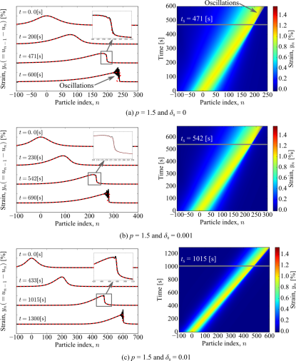
Figure 1: Strain wave propagation for $p=1.5$ and (a) $\delta_{0}=0$, (b) 0.001, and (c) 0.01. Left figures show temporal plots of strain waves. The black solid line is obtained from the direct simulation of the discrete model, and the red dashed line is the prediction based on Eq. (15) (i.e., the continuum model). Strain curves are offset to ease visualization (ticks in the vertical axis indicate 1.0). The inset shows the magnified view of the leading part at the predicted shock time. The right figures show space-time contour plots of strain wave propagation. The gray solid line indicates the predicted analytical shock wave time.

In Figs. 1 and 2, in addition to showing the dynamics of the original underlying lattice of Eq. (1), the prediction based on the theoretical analysis of the nonlinear transport PDE is shown, see Eq. (15). It can be inferred that the two closely match until the time where a discontinuity is about to form at which time the discrete model starts to feature oscillatory dynamics, a dispersive feature absent in the continuum, long wavelength model. A specific diagnostic in that connection that we use in order to compare the discrete and continuum cases is the shock formation time $T_{s}$. To obtain this time from the simulations, we examine the slope of the wave shape by calculating the sign of the differences of the strains between adjacent particles, and we define the shock wave time ($T_{S}$) when the sign changes multiple times, i.e., when the discrete character of the model prevents (the continuum) shock wave formation. The resulting comparison of $T_{s}$ is a principal quantitative finding of the present work.

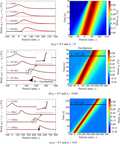
Figure 2: Strain wave propagation for $p=0.5$ and (a) $\delta_{0}=0$, (b) 0.001, and (c) 0.01. Left figures show temporal plots of strain waves. The black solid line is obtained from the direct simulation of the discrete model, and the red dashed line is the prediction based on Eq. (15) (i.e., the continuum model). Strain curves are offset to ease visualization (ticks in the vertical axis indicate 1.0). The inset shows the magnified view of the leading part at the predicted shock time. The right figures show space-time contour plots of strain wave propagation. The gray solid line indicates the predicted analytical shock wave time.

Figure 3 shows the comparison between numerical and analytical shock wave time for different exponent values ($p$). The difference increases if $p$ approaches unity because $p=1$ indicates that the system becomes a linear advection equation which does not support shock waves. It is for that reason that the shock formation time diverges as the limit $p\rightarrow 1$ is approached. Nevertheless, the quantitative trend between the two cases ($p>1$ and $p<1$) is well captured in both panels of the figure, i.e., for different values of the nonlinearity. In addition, we analyze the effect of pre-compression ($\delta_{0}$) on the shock wave time as shown in Fig. 4. As we increase the pre-compression (i.e., the system enters the weakly nonlinear regime and progressively approaches linear regime), the difference between numerical and analytical results increases. One can argue that this disparity may be partially related to the way we quantify $T_{s}$. In particular, as the system approaches $p=1$ or $\delta_{0}$ large, linear modes become progressively more accessible to it (a situation to be contrasted with the sonic vacuum where no such modes exist). As a result, while in the sonic vacuum – in the effective absence of linear modes – the time of the shock nearly coincides with the emergence of non-monotonicity near the wave front, in the progressively nearer linear case, the non-monotonicity emerges earlier. Hence the numerical evaluation of $T_{s}$ (based on the emergence of discreteness induced oscillations) suggests that $T_{s}$ is calculated to be well before the wave breaking event predicted by the analytics. Despite this distinction, it is fair to say that the quasi-continuum theory provides a very good tool for predicting the pre-shock wavefront evolution and for estimating the shock time, except in the vicinity of linear dynamical evolution.

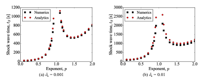
Figure 3: Effect of the exponent value ($p$) on the shock wave time for (a) $\delta_{0}=0.001$ and (b) $\delta_{0}=0.01$. The black square indicates the shock wave time from numerical simulations ($T_{S}$), and the red circle is the analytical prediction ($T_{s}$).

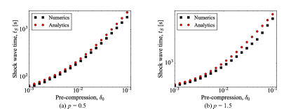
Figure 4: Effect of the pre-compression ($\delta_{0}$) on the shock wave time for (a) $p=0.5$ and (b) $p=1.5$. The black square indicates the shock wave time from numerical simulations ($T_{S}$), and the red circle is the analytical prediction ($T_{s}$). Data is plotted on log-log scale.

IV Conclusions & Future Challenges

In the present work, we have investigated shock and rarefaction wave formation in generalized granular crystal systems with Hertzian contacts. Motivated by recent developments in origami metamaterials Yasuda and Yang (2015); Yasuda et al. (2016) and tensegrity structures Fraternali et al. (2014), we explored both the scenario of $p>1$ (including $p=3/2$ of spherical contacts), and that of $p<1$ of strain-softening media. We identified the emergence of both shock waves and rarefaction waves and found a complementarity between the two cases. In the strain-hardening case, shock waves arise out of monotonically decreasing initial conditions while rarefactions out of monotonically increasing ones. The reverse occurs in the case of strain-softening $p<1$ media. The generalization of the quasi-continuum formulation of Chong et al. (2014) in the spirit of the nonlinear transport equations proposed by McDonald and Calvo (2012) provided us with an analytical handle in order to characterize the evolution of pulse-like data in the strain variables. A key quantitative prediction concerned the time of formation of the discontinuity as characterized at the quasi-continuum level. We discussed how the discreteness of the system, once visiting scales comparable to the lattice spacing, intervenes by generating oscillations and departing in this way from the quasi-continuum description.

This work suggests a number of exciting possibilities for the future. One interesting avenue is that of obtaining information about dispersive shock waves either at the level of the KdV model, or at that of the Toda lattice and then. Then, in the spirit of Shen et al. (2014), we can use these to characterize the formation of dispersive shock waves that emerge in the presence of precompression. That being said, it is unclear what becomes of such dispersive shock waves when precompression is weak or absent, as especially in the latter case there is no definitive characterization of dispersive shock waves. However, the direction of the first order equations could be an especially profitable one in that context. The work of Turner and Rosales (1997) (see also numerous important references therein) suggests that for the inviscid Burgers problem shock waves have been extensively studied both analytically and numerically. It is conceivable that a (judiciously selected) discretization of the first order PDEs considered herein could offer considerable insight in the formation of shock waves, both in the weak and even in the case of vanishing precompression limit. These are important directions that are under current consideration and will be reported in future publications.