Abstract

Invariance to nuisance transformations is one of the desirable properties of effective representations. We consider transformations that form a group and propose an approach based on kernel methods to derive local group invariant representations. Locality is achieved by defining a suitable probability distribution over the group which in turn induces distributions in the input feature space. We learn a decision function over these distributions by appealing to the powerful framework of kernel methods and generate local invariant random feature maps via kernel approximations. We show uniform convergence bounds for kernel approximation and provide generalization bounds for learning with these features. We evaluate our method on three real datasets, including Rotated MNIST and CIFAR-10, and observe that it outperforms competing kernel based approaches. The proposed method also outperforms deep CNN on Rotated-MNIST and performs comparably to the recently proposed group-equivariant CNN.

1 Introduction

Effective representation of data plays a key role in the success of learning algorithms. One of the most desirable properties of effective representations is being invariant to nuisance transformations. For instance, convolutional neural networks (CNNs) owe much of their empirical success to their ability in capturing local translation invariance through convolutional weight sharing and pooling which turns out to be a useful model prior for images. Capturing class sensitive invariance can also result in reduction in sample complexity [1] which is particularly useful in label scarce applications. We approach the problem of learning with invariant representations from a group theoretical perspective and propose a scalable framework for incorporating invariance to nuisance group actions via kernel methods.

At an abstract level, a group is defined as a set $G$ endowed with a notion of product on its elements that satisfies certain axioms of (i) closure: $a,b\in G\Longrightarrow$ the product $ab\in G$, (ii) associativity: $(ab)c=a(bc)$, and (iii) inverse element: for each $g\in G,\exists g^{-1}\in G$ such that $gg^{-1}=g^{-1}g=e\in G$, where $e$ is the identity element satisfying $ge=eg=g,\forall\,g\in G$. A group is abelian if the group product is commutative ($gh=hg,\forall\,g,h\in G$). For most practical applications each element $g\in G$ can be seen as a transformation acting on an input space $X$, $T_{g}:X\mapsto X$. The orbit of an element $x\in X$ under the action of the group $G$ is defined as the set $O_{x}=\{T_{g}(x)\mid g\in G\}$. The set of all rotations in a fixed 2-D plane is an example of an infinite group where the product is defined as the consecutive application of two rotations. The orbit of an image under this rotation group is the infinite set consisting of all rotated versions of the image. The closure property of the group implies that the orbit of a point $x$ is invariant under a group action on $x$, i.e., $O_{x\mid G}=O_{T_{g}(x)},\forall g\in G$. The reader is referred to [38] for a more detailed introduction to group theory.

For unimodular groups, which include compact groups and abelian groups, there exists a so called unique (up to scaling) Haar measure $\nu$ that is invariant to both left and right group products, i.e., $\nu(S)=\nu(gS)=\nu(Sg)$ for all measurable subsets $S\subset G$ and all $g\in G$, essentially generalizing the notion of Lebesgue measure to groups. For a compact group $G$, Haar measure can be normalized by $\nu(G)$ (since $\nu(G)<\infty$) to obtain the normalized Haar measure which assigns a probability mass to all measurable subsets of $G$. Normalized Haar measure can be seen as inducing a uniform probability distribution on the group. Recently, Anselmi et al. [1] used the normalized Haar measure $\tilde{\nu}$ on the group to map each orbit ($O_{x\mid G}\forall x$) to a probability distribution $P_{x}$ on the input space, i.e., $P_{x\mid G}(A)=\tilde{\nu}(\{g\mid T_{g}(x)\in A\}),\forall A\subset X$. The distribution $P_{x\mid G}$ induced by each point $x$ can be taken as its invariant representation. However, estimating this distribution directly can be challenging due to its potentially high dimensional support. Anselmi et al. [1] propose to capture histogram statistics of 1-dimensional projections of $P_{x\mid G}$ to generate an invariant representation that can be used for learning, i.e., $\phi_{n}^{k}(x)=1/|G|\sum_{g\in G}\eta_{n}(\langle T_{g}(x),t_{k}\rangle)$ for a finite group $G$, where $t_{k}$ are the projection directions (termed as templates), $\eta_{n}(\cdot)$ are some nonlinear functions that are expected to capture the histogram statistics. More recently, Mroueh et al. [31] analyzed the concentration properties of the linear kernel defined over these features and provided generalization bounds for learning with this linear kernel.

Our point of departure from [1, 31] is the observation that histogram based features may not be the optimal way to characterize the probability distributions $P_{x}$ induced by the group on the input space and their approach has its limitations. First, there is no principled guidance provided regarding the choice of nonlinearities $\eta_{n}$. Second, the inner-product of histogram based features ($\{\phi_{n}^{k}(x)\}$) approximately induces a Euclidean distance (group-averaged) in the input space [31] which may render them unsuitable for learning complex nonlinear decision boundaries in the input space. Further, locality is achieved by restricting the uniform distribution to a chosen subset of the group (i.e. elements within the subset are allowed to transform the input with equal probability and elements outside the subset are prohibited) which can be limiting.

Contributions: In this paper, we address aforementioned points and propose a framework to generate invariant representations by embedding the orbit distributions $P_{x\mid G}$ into a reproducing kernel Hilbert space (RKHS) [42, 33]. We propose to use characteristic kernels [44] so that the resulting map from the distributions to the RKHS is injective (one-to-one), preserving all the moments of the distribution. Our use of kernel methods to embed orbit distributions also renders a large body of work on kernel approximation methods at our disposal, which enable us to scale our proposed method. In particular, we derive invariant features by approximating the kernel using Nyström method [48, 17] and random Fourier features (for shift invariant kernels) [34]. The nonlinearities in the features ($\eta_{n}(\cdot)$) emerge in a principled manner as a by-product of the kernel approximation. The RKHS embedding framework also naturally allows us to use more general probability distributions on the group, apart from the uniform distribution. This allows us to have better control over selectivity of the derived features and also becomes a technical necessity when the group in non-compact. We experiment with three real datasets and observe consistent accuracy improvements over baseline random Fourier [34] and Nyström features [17] as well as over [31]. Further, on Rotated MNIST dataset [24] we outperform recent invariant deep CNN and RBM based architectures [43, 40], and perform comparably to the more recently proposed group equivariant deep convolutional nets [11].

2 Formulation

Let the input features belong to a set $X\subset\mathbb{R}^{d}$. A group element $g\in G$ acts on points from $\mathbb{R}^{d}$ through a map $T_{g}:\mathbb{R}^{d}\mapsto\mathbb{R}^{d}$, and we use a shorthand notation of $gx$ to denote $T_{g}(x)$. We use $gS$ to denote the action of a group element $g$ on the set $S$, i.e., $gS=\{T_{g}(x)\mid x\in S\subseteq X\}$. We take liberty in using the same notation to denote the product of a group element with a subset of the group, i.e., $gS=\{gh\mid h\in S\subset G\}$ and $Sg=\{hg\mid h\in S\subset G\}$.

2.1 RKHS embedding of Orbit distributions

As introduced in the previous section, the orbit of an element $x\in X$ under the action of the group $G$ is defined as the set $O_{x\mid G}=\{gx\mid g\in G\}$. For all unimodular groups there exists a Haar measure $\nu:S\mapsto\mathbb{R}_{+}$ which is invariant under left and right group product i.e., $\nu(S)=\nu(gS)=\nu(Sg)$ for all measurable subsets $S\subset G$ and all $g\in G$. Let $q(\cdot)$ be the probability density function of a distribution defined over $G$. This probability distribution over the group can be used to map each orbit $O_{x\mid G}$ to a probability distribution $P_{x\mid G}$ on the input space, i.e., $P_{x\mid G}(A)=\int_{g:gx\in A}q(g)\,d\nu(g)\,\,\forall A\subset X$. Note that $P_{x\mid G}(O_{x\mid G})=1$ (for an appropriately normalized measure $\nu$), and $P_{x\mid G}(A)=0\,\forall\,A$ for which $A\cap O_{x\mid G}=\emptyset$.

Let $\mathcal{H}$ be a reproducing kernel Hilbert space (RKHS) of functions $f:X\mapsto\mathbb{R}$ induced by kernel $k:X\times X\mapsto\mathbb{R}$, with the inner-product satisfying the reproducing property, i.e., ${\langle}f,k(x,\cdot){\rangle}=f(x),\forall f\in\mathcal{H}$ and ${\langle}k(x,\cdot),k(x^{\prime},\cdot){\rangle}=k(x,x^{\prime})$. The RKHS embedding of the distribution $P_{x\mid G}$ is given as [42]

$$\mu[P_{x\mid G}]:=E_{z\sim P_{x\mid G}}k(z,\cdot).$$ (1)

This expectation is well-defined under the probability measure $P_{x\mid G}$, which is in turn induced by the measure $\nu$ over the group. The support of $P_{x\mid G}$ is $O_{x\mid G}$ and sampling a point $z\sim P_{x\mid G}$ is equivalent to sampling the corresponding group element $g$ and setting $z=gx$. Thus we can rewrite the RKHS embedding of Eq. 1 as

$$\mu[P_{x\mid G}]=\int_{G}k(gx,\cdot)q(g)\,d\nu(g).$$ (2)

If the kernel is characteristic this map from distributions to the RKHS is injective, preserving all the information about the distribution [44]. All universal kernels [46] are characteristic when the support set of the distribution is compact [42]. In addition, many shift invariant kernels (e.g., Gaussian and Laplacian kernels) are characteristic on all of $\mathbb{R}^{d}$ [18]. For precise characterization of characteristic shift invariant kernels, please refer to [45].

For a characteristic kernel the embedding $\mu[P_{x\mid G}]$ can be used as a proxy for $P_{x\mid G}$ in learning problems. To this end, we introduce a hyperkernel $h:\mathcal{H}\times\mathcal{H}\mapsto\mathbb{R}$ that defines the similarity between the RKHS embeddings corresponding to two points $x$ and $x^{\prime}$ as $k_{q,G}(x,x^{\prime}):=h(\mu[P_{x\mid G}],\mu[P_{x^{\prime}\mid G}])$. If we take $h$ to be the linear kernel which is the regular inner-product in $\mathcal{H}$, we obtain

$$\begin{split}k_{q,G}(x,x^{\prime})&:={\langle}\,\mu[P_{x\mid G}],\mu[P_{x^{\prime}\mid G}]\,{\rangle}_{\mathcal{H}}\\ &=\int_{G}\int_{G}k(gx,g^{\prime}x^{\prime})q(g)q(g^{\prime})d\nu(g)d\nu(g^{\prime})\end{split}$$ (3)

The kernel $k_{q,G}:X\times X\mapsto\mathbb{R}$ turns out to be the expectation of the base kernel $k(\cdot,\cdot)$ under the predefined probability distribution on the group $G$. It trades off locality and group invariance through appropriately selecting the probability density $q(\cdot)$. Taking $q$ to be a delta function over the Identity group element gives back the original base kernel $k(\cdot,\cdot)$ which does not capture any invariance. On the other hand, if we take $q$ to be the uniform probability density, we get the global group invariant kernel (also termed as Haar integration kernel [21, 31])

$$k_{G}(x,x^{\prime})=\int_{G}\int_{G}k(gx,g^{\prime}x^{\prime})d\nu(g)d\nu(g^{\prime}),$$ (4)

satisfying the property $k_{G}(gx,g^{\prime}x^{\prime})=k_{G}(x,x^{\prime})$ for any $g,g^{\prime}\in G$ and any $x,x^{\prime}\in X$. Haar integral kernel does not preserve any locality information (e.g., images of digits $6$ and $9$ will be placed under same equivalence class). Strictly speaking, we only need $\nu$ to be the normalized right Haar measure satisfying $\nu(S)=\nu(Sg),\,\forall\,S\subset G,\,\forall\,g\in G$ for the global group invariance property to hold. A unique (up to scaling) right Haar measure exists for all locally compact groups and for all unimodular groups (for which left and right Haar measures conincide) [38]. All Lie groups (e.g., rotation, translation, scaling, affine) are locally compact. Additionally, all compact groups (e.g., rotation), abelian groups (e.g., translation, scaling), and discrete groups (e.g., permutation) are unimodular. However, the Haar integration kernel $k_{G}(x,x^{\prime})$ of Eq. 4 can only be defined for compact groups since we need $\nu(G)<\infty$ to keep the integral finite. Indeed, earlier work has used Haar integration kernel for compact groups [21, 31] (however, without the RKHS embedding perspective provided in our work which motivates the use of a characteristic base kernel $k(\cdot,\cdot)$).

A framework allowing more general (non-uniform) probability distribution on the group serves two purposes: (i) It enables us to operate with non-compact groups in a principled manner since we only need $\int_{G}q(g)d\nu(g)<\infty$ to enable construction of kernels such that Eq. 3 is finite; (ii) It allows for a better control over locality of the kernel $k_{q,G}(\cdot,\cdot)$. Earlier work [1, 31] achieves locality by taking a subset $G_{0}\subset G$ and restricting the domain of the Haar integration kernel to be $G_{0}$ which amounts to having a uniform distribution over $G_{0}$. A more general non-uniform distribution (e.g., a unimodal distribution with mode at the Identity element of the group) allows us to smoothly decrease the probability of sampling more extreme group transformations rather than abruptly prohibiting group transforms falling outside a preselected subset.

2.2 Feature generation via kernel approximation

The kernel $k_{q,G}$ of Eq. 3 can be used for learning with kernel machines [41], probabilistically trading off locality and group invariance through appropriately selecting $q(\cdot)$. However, kernel based learning algorithms suffer from scalability issues due to the need to compute kernel values for all pairs of data points. In this section, we describe our approach to obtain local invariant features via approximating $k_{q,G}$.

2.2.1 Features using random Fourier approximation

We first consider the case of shift-invariant base kernel satisfying $k(x,x^{\prime})=\tilde{k}(x-x^{\prime})$ which is a commonly used class of kernels that includes Gaussian and Laplacian kernels. Many shift-invariant kernels are characteristic on $\mathbb{R}^{d}$ as mentioned in the previous section. We use the random Fourier features proposed in [34] that are based on the characterization of positive definite functions by Bochner [6, 39]. Bochner’s theorem establishes Fourier transform as a bijective map from finite non-negative Borel measures on $\mathbb{R}^{d}$ to positive definite functions on $\mathbb{R}^{d}$. Applying it to shift-invariant positive definite kernels one gets

$$k(x,x^{\prime})=\tilde{k}(x-x^{\prime})=\int_{\mathbb{R}^{d}}e^{-i(x-x^{\prime})^{\top}\omega}p(\omega)d\omega,\,\forall\,x,x^{\prime},$$ (5)

where $p(\cdot)$ is the unique probability distribution corresponding to the kernel $k(\cdot,\cdot)$, assuming the kernel is properly scaled. We use this characterization to obtain local group invariant features as follows:

$$k_{q,G}(x,x^{\prime})$$

$$=\int_{G}\int_{G}E_{\omega\sim p}\left[e^{-i(gx-g^{\prime}x^{\prime})^{\top}\omega}\right]q(g)q(g^{\prime})d\nu(g)d\nu(g^{\prime})$$

$$=E_{\omega\sim p}\int_{G}\int_{G}e^{-i(gx-g^{\prime}x^{\prime})^{\top}\omega}q(g)q(g^{\prime})d\nu(g)d\nu(g^{\prime})$$

$$=E_{\omega\sim p}\int_{G}e^{-i{\langle}\omega,gx{\rangle}}q(g)d\nu(g)\int_{G}e^{i{\langle}\omega,g^{\prime}x^{\prime}{\rangle}}q(g^{\prime})d\nu(g^{\prime})$$

$$\approx E_{\omega\sim p}\frac{1}{r^{2}}\sum_{k=1}^{r}e^{-i{\langle}\omega,g_{k}x{\rangle}}\sum_{k=1}^{r}e^{i{\langle}\omega,g_{k}x{\rangle}},\quad(g_{k}\sim q)$$

$$\approx\frac{1}{sr^{2}}\sum_{j=1}^{s}\sum_{k=1}^{r}e^{-i{\langle}\omega_{j},g_{k}x{\rangle}}\sum_{k=1}^{r}e^{i{\langle}\omega_{j},g_{k}x{\rangle}},\,\,(g_{k}\sim q,\omega_{j}\sim p)$$

$$:=\langle\psi_{RF}(x),\psi_{RF}(x^{\prime})\rangle_{\mathbb{C}^{s}},$$ (6)

where

$$\begin{split}\psi_{RF}(x)&=\frac{1}{r\sqrt{s}}\left[\sum_{k=1}^{r}e^{-i{\langle}\omega_{1},g_{k}x{\rangle}}\ldots\sum_{k=1}^{r}e^{-i{\langle}\omega_{s},g_{k}x{\rangle}}\right]\\ &\in\mathbb{C}^{s}.\end{split}$$ (7)

We use standard Monte Carlo to approximate both inner integral over the group and the outer expectation over $\omega$. It is also possible to use quasi Monte Carlo approximation for the expectation over $\omega$, which has been carefully studied for random Fourier features [49]. We provide uniform convergence bounds and excess risk bounds for these features in Section 3.

The feature map $\psi_{RF}(\cdot)$ requires us to apply $r$ group actions to every data point which can be expensive in large data regime. If the group action is unitary transformation preserving norms and distances between points (i.e., $\lVert gx\rVert_{2}=\lVert x\rVert_{2}$), the inner product satisfies ${\langle}x,x^{\prime}{\rangle}={\langle}gx,gx^{\prime}{\rangle}$. This can be used to transfer the group action from the data to the sampled template as ${\langle}\omega,gx{\rangle}={\langle}g^{-1}\omega,g^{-1}gx{\rangle}={\langle}g^{-1}\omega,x{\rangle}$ [1] without affecting the approximation of kernel $k_{q,G}$, as long as the pdf $q$ is symmetric around the identity element ($q(g)=q(g^{-1})\,\forall g\in G$). For instance, in the case of images which can be viewed as a function $I:\mathbb{R}^{2}\mapsto\mathbb{R}$, one can show the following result regarding group actions (e.g., rotation, translation, scaling, affine transformation).

Lemma 2.1.

Let $g$ be a group element acting on an image $I:\mathbb{R}^{2}\mapsto\mathbb{R}$. The group action defined as $T_{g}[I(x)]=\lvert J_{g}\rvert^{-1/2}I(g^{-1}x),\,\forall\,x$, where $J_{g}$ is the Jacobian of the transformation, is a unitary transformation and satisfies ${\langle}T_{g}(I),T_{g}(I^{\prime}){\rangle}={\langle}I,I^{\prime}{\rangle}$.

Proof.

See appendix. ∎

The lemma suggests scaling the pixel intensities of the image by a factor $\lvert J_{g}\rvert^{-1/2}$ to make the group action unitary. The Jacobian for rotating or translating an image has determinant $1$ obviating the need for scaling. For general affine transformation, we need to scale the pixel intensities accordingly to keep it unitary.

2.2.2 Features using Nyström approximation

Here we consider the case of a general base kernel and derive local group invariant features using Nyström approximation [48, 17]. Nyström method starts with identifying a set of landmark points (also referred as templates) $Z=\{z_{1},\ldots,z_{s}\}$ and approximates each function $f\in\mathcal{H}$ by its orthogonal projection onto the subspace spanned by $\{k(\cdot,z_{i})\}_{i=1}^{s}$. Several schemes for identifying the landmark points have been studied in the literature, including random sampling, sampling based on leverage scores, and clustering based landmark selection [23, 20]. We can choose landmarks from the original set $X$ or from the orbit $gX$. Nyström method approximates the kernel as $k(x,x^{\prime})\approx K_{Z,x}^{\top}K_{Z,Z}^{+}K_{Z,x^{\prime}}$, where $K_{Z,x}=[k(x,z_{1}),\ldots,k(x,z_{s})]^{\top}$ and $K_{Z,Z}$ is square kernel matrix for the landmark points with $K_{Z,Z}^{+}$ denoting the pseudo-inverse.

Since $K_{Z,Z}$ is a positive semi-definite matrix, let $K_{Z,Z}^{+}=L^{\top}L$, where $L\in\mathbb{R}^{\text{rank}(K_{Z,Z})\times s}$. We have

$$k_{q,G}(x,x^{\prime})$$

$$\approx\int_{G}\int_{G}K_{gx,Z}K_{Z,Z}^{+}K_{Z,g^{\prime}x^{\prime}}\,q(g)q(g^{\prime})d\nu(g)d\nu(g^{\prime})$$

$$=\int_{G}\int_{G}K_{gx,Z}L^{\top}LK_{Z,g^{\prime}x^{\prime}}\,q(g)q(g^{\prime})d\nu(g)d\nu(g^{\prime})$$

$$=\left\langle\int_{G}LK_{Z,gx}\,q(g)d\nu(g),\int_{G}LK_{Z,gx^{\prime}}\,q(g)d\nu(g)\right\rangle$$

$$\approx\left\langle L\frac{1}{r}\sum_{k=1}^{r}K_{Z,g_{k}x}\,,L\frac{1}{r}\sum_{k=1}^{r}K_{Z,g_{k}x^{\prime}}\right\rangle,\quad(g_{k}\sim q),$$

where the features are given by

$$\psi_{Nys}(x)=\frac{1}{r}L\sum_{k=1}^{r}K_{Z,g_{k}x}\,\,\in\mathbb{R}^{\text{rank}(K_{Z,Z})}.$$ (8)

If the base kernel satisfies $k(gx,gx^{\prime})=k(x,x^{\prime}),\,\forall\,g,x,x^{\prime}$, we can transfer the group action from the data points to the landmark points as $k(gx,z)=k(g^{-1}gx,g^{-1}z)=k(x,g^{-1}z)$ without affecting the Nyström approximation of $k_{q,G}$, as long as the pdf $q$ is symmetric around the identity element ($q(g)=q(g^{-1})\,\forall g\in G$). This becomes essential in large data regime where the number of data points is much larger than the number of landmarks. For the group action defined in Lemma 2.1, all dot product kernels ($\tilde{k}({\langle}x,x^{\prime}{\rangle})$) and shift invariant kernels ($\tilde{k}(\lVert x-x^{\prime}\rVert_{2})$) satisfy this property.

Remarks:
(1) Earlier work [1, 31] has proposed features of the form $\phi_{n}^{k}(x)=1/r\sum_{j=1}^{r}\eta_{n}(\langle g_{j}x,\omega_{k}\rangle)$ where $\eta_{n}(\cdot)$ were taken to be step functions $\eta_{n}(a)={1}(a<h_{n})$ with preselected thresholds $h_{n}$. Nonlinearities in our proposed local invariant features emerge naturally as a result of kernel approximation, with $\eta(x,\omega)=e^{-i{\langle}x,\omega{\rangle}}$ for $\psi_{RF}$ and $\eta(x,\omega)=k(x,\omega)$ for $\psi_{Nys}$.
(2) Our work can also be viewed as incorporating local group invariance in widely used random Fourier and Nyström approximation methods, however this viewpoint overlooks the Hilbert space embedding perspective motivated in this work.
(3) The kernel $k_{q,G}$ defined in Eq. (3) assumes a linear hyperkernel $h:\mathcal{H}\times\mathcal{H}\mapsto\mathbb{R}$ over RKHS embeddings of orbit distributions. It is also possible to use a nonlinear hyperkernel along the lines of [10] and [32], and approximate it using a second layer of random Fourier (RF) or Nyström features. We show empirical results for both linear and Gaussian hyperkernel (approximated using RF features) in Sec. 4.
(4) Computational aspects. The complexity of feature computation is $rC_{f}+rsC_{g}$ where $C_{f}$ is the cost of computing the vanilla random Fourier or vanilla Nyström features and $C_{g}$ is the cost of computing a group action on a template $\omega$. However same set of templates are used for all data points so group actions on the templates can be computed in advance. Structured random Gaussian templates can also be used in our framework to speed up the computation of random Fourier features $\psi_{RF}$ [25, 9, 7]. Recent approaches for scaling randomized kernel machines to massive data sizes and very large number of random features can also be used [3].

3 Theory

In this section we focus on local invariance learning using the random feature map $\psi_{RF}$ defined in Section 2.2.1 for the Gaussian base kernel $k(\cdot,\cdot)$. We first address the uniform convergence of the random feature map $\psi_{RF}$ to the local invariant kernel $k_{q,G}$ on a set of points $\mathcal{M}$. In other words we show in Theorem 3.1 that for a sufficiently large number of random templates $s$, and group element samples $r$, we have $\langle\psi_{RF}(x),\psi_{RF}(y)\rangle\approx k_{q,G}(x,y)$, for all points $x,y\in\mathcal{M}$. Second we consider a supervised binary classification setting, and study generalization bounds of learning a linear classifier in the local invariant random feature space $\psi_{RF}$. In a nutshell Theorem 3.2 shows that linear functions in the random feature space $\langle w,\psi_{RF}(x)\rangle$, approximate functions in the RKHS induced by our local invariant kernel $k_{q,G}$.

3.1 Uniform Convergence

Theorem 3.1 provides a uniform convergence bound of our invariant random feature map $\psi_{RF}$ for Gaussian base kernel $k(\cdot,\cdot)$.

Theorem 3.1 (Uniform convergence of Fourier Approximation).

Let $X$ be a compact space in $\mathbb{R}^{d}$ with diameter $\operatorname{diam}(X)$. For $\varepsilon>0,\delta_{1},\delta_{2}\in(0,1)$, the following uniform convergence bound holds with probability $1-\Big{(}\frac{64(d+1)}{\varepsilon^{2}\sigma^{2}}\Big{)}^{\frac{d}{d+1}}(\delta_{1}+\delta_{2})^{\frac{2d}{d+1}}.$

$$\underset{x,y\in X}{\sup}\Big{|}\Big{\langle}\psi_{RF}(x),\psi_{RF}(y)\Big{\rangle}-K_{q,G}(x,y)\Big{|}\leq\varepsilon+\frac{1}{r}$$

for a number of group samples

$$r\geq C_{1}\frac{d}{\varepsilon^{2}}\log(\rm{diam}(X)/\delta_{1}),$$

and a number of random templates

$$s\geq C_{2}\frac{d}{\varepsilon^{2}}\log(\rm{diam}(X)/\delta_{2}),$$

where $\sigma_{p}^{2}\equiv E_{p}[\omega^{\top}\omega]=d/\sigma^{2}$ is the second moment of the Fourier transform of the Gaussian base kernel $k$, and $C_{1}$ and $C_{2}$ are numeric universal constants.

Proof.

See Appendix. ∎

3.2 Generalization Bounds

Given a labeled training set $S\ =\big{\{}(x_{i},y_{i})\,|\,x_{i}\in X,y_{i}\in Y=\{+1,-1\}\big{\}}$, our goal is to learn a decision function $f:\ X\rightarrow Y$ via empirical risk minimization (ERM)

$$\min_{f\in\mathcal{H}_{\mathcal{K}}}\hat{\mathcal{E}}_{V}(f)=\frac{1}{N}\sum_{i=1}^{N}V(y_{i}f(x_{i}))$$

where $V$ is convex and $L$-Lipschitz loss function. Let $\mathcal{E}_{V}(f)=\mathbb{E}_{x,y\sim P}V(yf(x))$ be the expected risk for $f\in\mathcal{H_{K}}$. According to the representer theorem, the solution of ERM is given by $f^{\star}(\cdot)=\sum_{i=1}^{N}\alpha_{i}^{\star}k_{q,G}(x_{i},.)$.

We consider linear hyperkernel $h$ in Eq. (3) and consider $\mathcal{H}_{\mathcal{K}}$, the RKHS induced by the kernel $k_{q,G}(x,y)=\int_{G}\int_{G}k(gx,g^{\prime}x^{\prime})\,q(g)q(g^{\prime})\,d\nu(g)d\nu(g^{\prime})$, as introduced in Sec. 2.1. Similar to [31], for $C>0$, we define $\mathcal{F}_{p}$ an infinite dimensional space to approximate $\mathcal{H}_{\mathcal{K}}$ (see [35] for a motivation for this approximation):

$$\mathcal{F}_{p}\equiv\Big{\{}f(x)=\int_{\Omega}\alpha(\omega)\int_{G}\phi(gx,\omega)q(g)d\nu(g)d\omega\Big{|}$$

$$|\alpha(\omega)|\leq Cp(\omega)\Big{\}},$$

where $\phi(gx,\omega)=e^{-i{\langle}gx,\omega{\rangle}}$. Similarly define the linear space in the span of $\psi_{RF}(\cdot)$, $\mathcal{\hat{F}}_{p}\equiv\Big{\{}\hat{f}(x)=\langle\alpha,\psi_{RF}(x)\rangle=\sum_{k=1}^{s}\alpha_{k}\frac{1}{r}\sum_{i=1}^{r}\phi(g_{i}x,\omega_{k})\Big{|}|\alpha_{k}|\leq\frac{C}{s}\Big{\}}$.

Theorem 3.2.

Let $\delta>0$.Consider the training set $S\ =\ \big{\{}(x_{i},y_{i})\ |\ x_{i}\ \in X,y_{i}\ \in Y,i=1\ldots N\big{\}}$ sampled from the input space and let $f_{N}^{\star}$ is the empirical risk minimizer such that $f_{N}^{\star}\ =\mathop{\rm arg\,min}_{f\in\hat{\mathcal{F}}}\hat{\mathcal{E}}_{V}(f)=\frac{1}{N}\sum_{i=1}^{N}V(y_{i}f(x_{i}))$, then we have with probability $1-3\delta$ (over the training set, random templates and group elements)

$${\mathcal{E}_{V}}(f^{\star}_{N})-\min_{f\in\mathcal{F}_{P}}{\mathcal{E}_{V}}(f)\leq$$

$$\mathcal{O}\left(\left(\frac{1}{\sqrt{N}}+\frac{1}{\sqrt{s}}+\frac{1}{\sqrt{r}}\right)LC\sqrt{\log\frac{1}{\delta}}\right).$$

Proof.

See Appendix. ∎

4 Empirical Observations

We evaluate the proposed method (referred as LGIKA  here) on three real datasets. We use Gaussian kernel as the base kernel in all our experiments. For methods that produce random (unsupervised) features, which include the proposed approach as well as regular random Fourier (abbrv. as RF) [34] and Nystrom [48] method, we report performance with: (i) linear decision boundary on these features (linear SVM or linear regularized least squares (RLS)), and (ii) nonlinear decision boundary which is realized by having a Gaussian kernel on top of the features and approximating it through random Fourier features [34], followed by a linear SVM or RLS. The later can also be viewed as using a nonlinear hyperkernel over RKHS embeddings of orbit distributions (also see Remark (3) at the end of Sec. 2). Parameters for all the methods are selected using grid search on a hold-out validation set unless otherwise stated.

	RMSE	RMSE w/
Method		2nd layer RF
Original (RF)	14.01	13.78
Original (Nys)	13.97	13.81
Original (GP)	13.48	N/A
Sort-Coulomb (RF)	12.89	12.49
Sort-Coulomb (Nys)	12.83	12.51
Sort-Coulomb (GP)[30]	12.59	N/A
Rand-Coulomb[30]	11.40	N/A
GICDF [31]	12.25	N/A
LGIKA(RF)	10.82	10.05
LGIKA(Nys)	10.87	10.45

Table 1: RMSE on Quantum Machine data

4.1 Quantum Machine dataset

This data consists of $7165$ Coulomb matrices of size $23\times 23$ (each matrix corresponding to a molecule) and their associated atomization energies in kcal/mol. It is a small subset of a large dataset collected by Blum and Reymond (2009) [4], and was recently used by Montavon et al. (2012) [30] for evaluation. The goal is to predict atomization energies of molecules which is modeled as a regression task.

The atomization energy is known to be invariant to permutations of rows/columns of the Coulomb matrix which motivates the use of representations invariant to the permutation group. We follow the experimental methodology of [30] and report mean cross-validation accuracy on the five folds provided in the dataset. An inner cross-validation is used for tuning the parameters for each fold as in [30]. We compare the performance of our method with several baselines in Table 1: (i) Original (GP/RF/Nys): Gaussian Process regression on original Coulomb matrices and its approximation via random Fourier (RF) [34] and Nystrom features [48], (ii) Sort-Coulomb (GP/RF/Nys): GP regression on sorted Coulomb matrices (sorted according to row norms) [30] and its approximation, (iii) Rand-Coulomb: permutation invariant kernel proposed in [30], and (iv) GICDF: Group invariant CDF (histogram) based features proposed in [31]. The results for Sort-Coulomb (GP) and Rand-Coulomb are taken directly from [30]. For all RF and Nyström based features we use $10k$ random templates ($\omega$). For GICDF and our method, we sample $70$ random permutations ($r=70$ in Eq. 7) using the same scheme as in [30]. The proposed LGIKA  outperforms all these directly competing methods including Rand-Coulomb and GICDF. Neural network based features used in [30] can also be used within our framework but we stick to raw Coulomb matrices for simplicity sake.

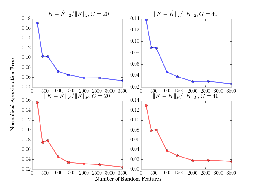
Figure 1: Kernel approximation error (normalized) in spectral and Frobenius norms vs number of random features, for $20$ (left) and $40$ (right) group transformations

Kernel Approximation. We also report empirical results on approximation error for kernel matrix (in terms of spectral norm and Frobenius norm) in Fig. 1. The plots show the approximation error for different number of group actions as the number of random Fourier features are increased. The kernel used is the Gaussian kernel. The true kernel has been computed using $70$ group elements randomly sampled from the permutation group. The normalized error for all the cases goes down with the number of random Fourier features which is in line with our theoretical convergence results.

	Accuracy	Accuracy w/
Method		2nd layer RF
Original (RF)	87.75	88.01
Original (Nys)	88.93	88.98
Original (RBF)	90	N/A
TI-RBM [43]	95.8	N/A
RC-RBM [40]	97.02	N/A
GICDF [31]	93.81	N/A
Z2-CNN [11]	94.97	N/A
P4-CNN [11]	97.72	N/A
LGIKA(RF)	96.83	97.18
LGIKA(Nys)	96.81	97.21

Table 2: Rotated MNIST results

4.2 Rotated MNIST

Rotated MNIST dataset [24] consists of total $62k$ images of digits ($12k$ for training and $50k$ for test), obtained by rotating original MNIST images by an angle sampled uniformly between $0$ and $2\pi$. We compare the proposed method with several other approaches in Table 2. We use von-misses distribution ($p(\theta)=\exp(-\kappa\cos(\theta))$ with $\kappa=0.2$, selected using cross-validation) to sample $r=100$ rotations. We use $s=7k$ random templates for both RF and Nystrom approximations, and use $17k$ random templates for layer-2 RF approximation. The results for the cited methods in Table 2 are directly taken from the respective papers, except for GICDF [31] which we implemented ourselves. The proposed LGIKA  outperforms most of the competing methods including deep architectures like rotation-invariant convolutional RBM (RC-RBM) [40], transformation invariant RBM (TI-RBM) [43], and regular deep CNN (Z2-CNN) [11]. Our method also performs close to the recently proposed group-equivariant CNN (P4-CNN) [11].

4.3 CIFAR-10

The CIFAR-10 dataset consists of $60k$ RGB images ($50k/10k$ for train/test) of size $32\times 32$, divided into 10 classes. We consider a sub-group of the affine group $Aff(2)$ consisting of rotations, translations and isotropic scaling. Instead of operating with a distribution (e.g. Gaussian) over this subgroup, we use three individual distributions to have better control over the three variations: a log-normal distribution over the scaling group ($\mu=0,\sigma=0.3$), a Gaussian distribution over the translation group ($\mu=0,\sigma=0.3$), and a von-misses distribution over the rotation group ($\kappa=9$). We observe that working with wider distributions over these groups actually hurts the performance, highlighting the importance of locality for CIFAR-10. We use the normalized pixel intensities as our input features and use the group action defined in Lemma 2.1 to keep it unitary. We use $s=10k$ random templates and $r=50$ group transforms for the first layer RF features (Eq. 7), and use $30k$ random templates for second layer RF features. The proposed LGIKA outperforms vanilla RF features as shown in Table 3. Nyström based features gave similar results as random Fourier features in our early explorations. We were not able to scale GICDF [31] to a suitable number of random templates due to memory issues (for every random template, GICDF generates $n$ features (number of bins, set to $25$ following [31]) blowing up the overall feature dimension to $n\times 10k$). Note that the performance of LGIKA on this data is still significantly worse than deep CNNs [11] since LGIKA treats the image as a vector ignoring the spatial neighborhood structure taken into account by CNNs through translation invariance over small image patches. Incorporating orbit statistics of image patches in our framework is left for future work.

Original (RF) [34]		LGIKA
1-layer	2-layer	1-layer	2-layer
61.02	62.79	64.19	67.32

Table 3: CIFAR-10 results

5 Related Work

Invariant Kernel Methods. [2] introduced Tomographic Probabilistic Representations (TPR) that embed orbits to probability distributions. Unlike TPR, our representation maps orbits or local portions of the orbit via kernel mean embedding to an RKHS and allows to define similarity between orbits in this space. Indeed our representation is infinite dimensional and is related to Haar Invariant Kernel [21]. As discussed earlier it can be approximated via random features or Nyström sampling. Other approaches for building invariant kernels were defined in [47] that focuses on dilation invariances. A kernel view of histogram of gradients was introduced in [5], where finite dimensional features were defined through kernel PCA. Kernel convolutional networks introduced in [29],[28], considers the composition of multilayer kernels, where local image patches are represented as points in a reproducing kernel. However they do not consider general group invariances. The work of [13] considers the general problem of learning from conditional distributions. When applied to invariant learning, their optimization approach needs to sample a group transformed example in every SGD iteration whereas our approach allows working with group actions on the random templates.
Invariance in Neural Networks. Inducing invariances in neural networks has attracted many recent research streams. It is now well established that convolutional neural networks (CNN) [26] ensure translation invariance. [16] showed that mapping orbits of rotated and flipped images through a shared fully connected network builds some invariance in the network. Scattering networks [8] have built in invariances for the roto-translation group. [19] generalizes CNN to general group transformations. [15] exploits cyclic symmetry to have invariant prediction in the network. More recently, [11] designs a convolutional neural network that is equivariant to group transforms by introducing convolution over the group.

6 Concluding Remarks

The proposed approach can be suitable for large-scale problems, benefiting from the recent advances in scalability of randomized kernel methods [27, 14, 3]. As a future direction, we would like to extend our framework to operate at the level of image patches, enabling us to capture local spatial structure. Further, the proposed approach requires computation of all $r$ group transformations for all the sampled random templates. Reducing the required number of group transformations is an important direction for future work. Our work also assumes that the appropriate group actions are given. Extension to the case when the group transformations are learned from the data (e.g., using local tangent space [37]) is also an important direction for future work.

Acknowledgments: We thank Dmitry Malioutov for several insightful discussions. This work was done while Anant Raj was a summer intern at IBM Research.

Appendix

Proof of Lemma 2.1.

Since unitary transformations preserve dot-products, i.e., ${\langle}T(x),T(y){\rangle}={\langle}x,y{\rangle}$, we need to show that a group element acting on the image $I:\mathbb{R}^{2}\mapsto\mathbb{R}$ as $T_{g}[I(x)]=\lvert J_{g}\rvert^{-1/2}I(T_{g}^{-1}(x)),\,\forall\,x$ is a unitary transformation.

Let $J_{g}$ be the Jacobian of the transformation $T_{g}$, with determinant $\lvert J_{g}\rvert$. We have

$$\lVert I(T_{g}^{-1}(\cdot))\rVert^{2} =\int I^{2}(T_{g}^{-1}(x))dx$$

$$=\int I^{2}(z)\,\lvert J_{g}\rvert\,dz,\quad\text{substituting }z=T_{g}^{-1}(x)\Rightarrow dx=\lvert J_{g}\rvert\,dz$$

$$=\lvert J_{g}\rvert\,\lVert I(\cdot)\rVert^{2}$$

Hence the transformation given as $T_{g}[I(\cdot)]=\lvert J_{g}\rvert^{-1/2}I(T_{g}^{-1}(\cdot))$ is unitary and thus ${\langle}T_{g}(I),T_{g}(I^{\prime}){\rangle}={\langle}I,I^{\prime}{\rangle}$ for two images $I$ and $I^{\prime}$. ∎

Proof of Theorem 3.1.

We first define the notion of U-statistics [22].

U-statistics - Let $g:\mathbb{R}^{2}\rightarrow\mathbb{R}$ be a symmetric function of its arguments. Given an i.i.d. sequence $X_{1},X_{2}\cdots X_{k}$ of $k(\geq 2)$ random variables, the quantity $U:=\frac{1}{n(n-1)}\sum_{i\neq j,i,j=1}^{n}g(X_{i},X_{j})$ is known as a pairwise U-statistics. If $\theta(P)=\mathbb{E}_{X_{1},X_{2}\sim P}\,g(X_{1},X_{2})$ then $U$ is an unbiased estimate of $\theta(P)$.

Our goal is to bound

$$\underset{x,y\in X}{\sup}\Big{|}\Big{\langle}\psi_{RF}(x),\psi_{RF}(y)\Big{\rangle}-k_{q,G}(x,y)\Big{|}$$

where

$$\psi_{RF}(x)=\frac{1}{r}\sum_{i=1}^{r}z(g_{i}x),x\in X\subset\mathbb{R}^{d}.$$

We work with $z(\cdot)=\sqrt{2/s}[\cos(\langle\omega_{1},\cdot\rangle+b_{1}),\ldots,cos(\langle\omega_{s},\cdot\rangle+b_{s}]\in\mathbb{R}^{s}$ with $b_{i}\sim\text{Unif}(0,2\pi)$ as in [34].

Let $\widehat{k}_{q,G}(x,y):=\frac{1}{r^{2}}\sum_{i,j=1}^{r^{2}}k(g_{i}x,g_{j}y)$ and $\widetilde{k}_{q,G}(x,y):=\frac{1}{r(r-1)}\sum_{i\neq j,i,j=1}^{r^{2}}k(g_{i}x,g_{j}y)$.

Using the triangle inequality we have

$$\underset{x,y\in X}{\sup}\Big{|}\Big{\langle}\psi_{RF}(x),\psi_{RF}(v)\Big{\rangle}-k_{q,G}(x,y)\Big{|}\leq\underbrace{\underset{x,y\in X}{\sup}\Big{|}\Big{\langle}\psi_{RF}(x),\psi_{RF}(y)\Big{\rangle}-\widehat{k}_{q,G}(x,y)\Big{|}}_{A}$$

$$\qquad\qquad\qquad\qquad\qquad\qquad+\underbrace{\underset{x,y\in X}{\sup}\Big{|}\widetilde{k}_{q,G}(x,y)-k_{q,G}(x,y)\Big{|}}_{B}+\underbrace{\underset{x,y\in X}{\sup}\Big{|}\widehat{k}_{q,G}(x,y)-\widetilde{k}_{q,G}(x,y)\Big{|}}_{C}$$

Bounding A.

$$A :=\sup_{x,y\in X}\Big{|}\frac{1}{r^{2}}\sum_{i,j}\left(\langle z(g_{i}x),z(g_{j}y)\rangle-k(g_{i}x,g_{j}y)\right)\Big{|}$$

Let us define $f_{ij}(x,y):=\langle z(g_{i}x),z(g_{j}y)\rangle-k(g_{i}x,g_{j}y)$, and $f(x,y)=1/r^{2}\sum_{i,j}f_{ij}(x,y)$. Since each of the $s$ independent random variables in the summand of $1/r^{2}\sum_{i,j}\langle z(g_{i}x),z(g_{j}y)\rangle=\frac{1}{s}\sum_{k=1}^{s}\bigg{(}\frac{1}{r^{2}}$ $\sum_{i,j}2\cos(\langle\omega_{k},g_{i}x\rangle+b_{k})$ $\cos(\langle\omega_{k},g_{j}y\rangle+b_{k})\bigg{)}$ is bounded by $[-2,2]$, using Hoeffding’s inequality for a given pair $x,y$, we have

$$\text{Pr}[|f(x,y)|\geq\varepsilon/4]\leq 2\exp(-s\varepsilon^{2}/128).$$

To obtain a uniform convergence guarantee over $X$, we follow the arguments in [34], relying on covering the space with an $\varepsilon$-net and Lipschitz continuity of the function $f(x,y)$.

Since $X$ is compact, we can find an $\varepsilon$-net that covers $X$ with $N_{X}=\left(\frac{2\,\rm{diam}(X)}{\eta}\right)^{d}$ balls of radius $\eta$ [12]. Let $\{c_{k}\}_{k=1}^{N_{X}}$ be the centers of these balls, and let $L_{f}$ denote the Lipschitz constant of $f(\cdot,\cdot)$, i.e., $|f(x,y)-f(c_{k},c_{l})|\leq L_{f}\lVert\left(\begin{smallmatrix}x\\ y\end{smallmatrix}\right)-\left(\begin{smallmatrix}c_{k}\\ c_{l}\end{smallmatrix}\right)\rVert$ for all $x,y,c_{k},c_{l}\in X$. For any $x,y\in X$, there exists a pair of centers $c_{k},c_{l}$ such that $\lVert\left(\begin{smallmatrix}x\\ y\end{smallmatrix}\right)-\left(\begin{smallmatrix}c_{k}\\ c_{l}\end{smallmatrix}\right)\rVert<\sqrt{2}\eta$. We will have $|f(x,y)|<\varepsilon/2$ for all $x,y$ if (i) $|f(c_{k},c_{l})|<\frac{\varepsilon}{4},\,\forall c_{k},c_{l}$, and (ii) $L_{f}<\frac{\varepsilon}{4\sqrt{2}\eta}$.

We immediately get the following by applying union bound for all the center pairs $(c_{k},c_{l})$

$$\text{Pr}\left[\cup_{k,l}|f(c_{k},c_{l})|\geq\varepsilon/4\right]\leq 2\,N^{2}_{X}\exp(-s\varepsilon^{2}/128).$$ (9)

We use Markov inequality to bound the Lipschitz constant of $f$. By definition, we have $L_{f}=\sup_{x,y}\lVert\nabla_{x,y}$ $f(x,y)\rVert=\lVert\nabla_{x,y}f(x^{*},y^{*})\rVert$, where $\nabla_{x,y}f(x,y)=\left(\begin{smallmatrix}\nabla_{x}f(x,y)\\ \nabla_{y}f(x,y)\end{smallmatrix}\right)$. We also have $\mathbb{E}_{\omega\sim p}\nabla_{x,y}\langle z($ $g_{i}x),z(g_{j}y)\rangle=\nabla_{x,y}k(g_{i}x,g_{j}y)$. It follows that

$$\mathbb{E}_{\omega\sim p}\left\lVert\nabla_{x,y}f(x^{*},y^{*})\right\rVert^{2} =\mathbb{E}_{\omega\sim p}\left\lVert\frac{1}{r^{2}}\sum_{i,j=1}^{r}\nabla_{x,y}\langle z(g_{i}x^{*}),z(g_{j}y^{*})\rangle\right\rVert^{2}-\left\lVert\frac{1}{r^{2}}\sum_{i,j=1}^{r}\nabla_{x,y}k(g_{i}x^{*},g_{j}y^{*})\right\rVert^{2}$$

$$\leq\mathbb{E}_{\omega\sim p}\left\lVert\frac{1}{r^{2}}\sum_{i,j=1}^{r}\nabla_{x,y}\langle z(g_{i}x^{*}),z(g_{j}y^{*})\rangle\right\rVert^{2}$$

$$\leq\mathbb{E}_{\omega\sim p}\left(\frac{1}{r^{2}}\sum_{i,j=1}^{r}\lVert\nabla_{x,y}\langle z(g_{i}x^{*}),z(g_{j}y^{*})\rangle\rVert\right)^{2}$$

$$\leq 2\mathbb{E}_{\omega\sim p}\sup_{x,y,g_{i},g_{j}}\lVert\nabla_{x}\langle z(g_{i}x),z(g_{j}y)\rangle\rVert^{2}$$

$$\leq 2\mathbb{E}_{\omega\sim p}\sup_{x,g}\left(\frac{1}{s}\sum_{k=1}^{s}\lVert\nabla_{x}T_{g}(x)\omega_{k}\rVert\right)^{2}$$

$$\leq 2\mathbb{E}_{\omega\sim p}\sup_{x,g}\left(\frac{1}{s}\sum_{k=1}^{s}\lVert\nabla_{x}T_{g}(x)\rVert_{2}\lVert\omega_{k}\rVert\right)^{2}$$

$$=2\mathbb{E}_{\omega\sim p}\sup_{x,g}\lVert\nabla_{x}T_{g}(x)\rVert_{2}^{2}\frac{1}{s^{2}}\sum_{k=1}^{s}\sum_{l=1}^{s}\lVert\omega_{k}\rVert\lVert\omega_{l}\rVert$$

$$=2\sup_{x,g}\lVert\nabla_{x}T_{g}(x)\rVert_{2}^{2}\frac{1}{s^{2}}\sum_{k=1}^{s}\sum_{l=1}^{s}\mathbb{E}_{\omega\sim p}\lVert\omega_{k}\rVert\lVert\omega_{l}\rVert$$

$$=2\sup_{x,g}\lVert\nabla_{x}T_{g}(x)\rVert_{2}^{2}\frac{1}{s^{2}}\left(s\mathbb{E}_{\omega\sim p}\lVert\omega\rVert^{2}+\sum_{k,l=1,k\neq l}^{s}(\mathbb{E}_{\omega\sim p}\lVert\omega\rVert)^{2}\right)\quad(\text{$\omega_{k}$ i.i.d.})$$

$$\leq 2\sup_{x,g}\lVert\nabla_{x}T_{g}(x)\rVert_{2}^{2}\frac{1}{s^{2}}\left(s\mathbb{E}_{\omega\sim p}\lVert\omega\rVert^{2}+\sum_{k,l=1,k\neq l}^{s}\mathbb{E}_{\omega\sim p}\lVert\omega\rVert^{2}\right)\quad(\text{Jensen's inequality})$$

$$\leq 2\sigma_{p}^{2}\sup_{x\in X,g\in G}\lVert\nabla_{x}T_{g}(x)\rVert_{2}^{2},$$

where $\sigma_{p}^{2}=\mathbb{E}(\omega^{\top}\omega)$, and $T_{g}(x)=gx$ denotes the transformation corresponding to the group action. If we assume the group action to be linear, i.e., $T_{g}(x+y)=T_{g}(x)+T_{g}(y)$ and $T_{g}(\alpha x)=\alpha T_{g}(x)$, which holds for all group transformations considered in this work (e.g., rotation, translation, scaling or general affine transformations on image $x$; permutations of $x$), we can bound $\lVert\nabla_{x}T_{g}(x)\rVert_{2}$ as

$$\lVert\nabla_{x}T_{g}(x)\rVert_{2} =\sup_{u:\lVert u\rVert=1}\lVert\nabla_{x}T_{g}(x)u\rVert$$

$$=\sup_{u:\lVert u\rVert=1}\left\lVert\lim_{h\to 0}\frac{T_{g}(x+hu)-T_{g}(x)}{h}\right\rVert\quad(\text{directional derivative of vector valued function }T_{g}(\cdot))$$

$$=\sup_{u:\lVert u\rVert=1}\lVert T_{g}(u)\rVert=1$$

$$\quad(\text{since }T_{g}(\cdot)\text{ is either unitary or is converted to unitary by construction (see Lemma 2.1)})$$

Using Markov inequality, $\text{Pr}[L_{f}^{2}\geq\varepsilon]\leq\mathbb{E}(L_{f}^{2})/\varepsilon$, hence we get

$$\text{Pr}\left[L_{f}\geq\frac{\varepsilon}{4\sqrt{2}\eta}\right]\leq\frac{64\sigma_{p}^{2}\eta^{2}}{\varepsilon^{2}}.$$

Combining Eq. (9) with the above result on Lipschitz continuity, we get

$$\text{Pr}\left[\sup_{x,y}|f(x,y)|\leq\varepsilon/2\right]\geq 1-2\,N^{2}_{X}\exp(-s\varepsilon^{2}/128)-\frac{64\sigma_{p}^{2}\eta^{2}}{\varepsilon^{2}}.$$ (10)

Bounding B.

As defined earlier, $\widetilde{k}_{q,G}(x,y):=\frac{1}{r(r-1)}\sum_{i\neq j,i,j=1}^{r}k(g_{i}x,g_{j}y)$. From the result of U-statistics literature [22], it is easy to see that $\mathbb{E}(\widetilde{k}_{q,G}(x,y))=k_{q,G}(x,y)$.
Since $g_{1},g_{2}\cdots g_{r}$ are i.i.d samples, we can consider $\widetilde{k}_{q,G}(x,y)$ as function of $r$ random variables $(g_{1},g_{2},\cdots g_{r})$. Denote $\widetilde{k}_{q,G}(x,y)$ as $f(g_{1},g_{2},\cdots g_{r})$ . Now if a variable $g_{p}$ is changed to $g^{\prime}_{p}$ then we can bound the absolute difference of the changed and the original function. For the rbf kernel, $|k(g_{p}x,g_{j}y)-k(g^{\prime}_{p}x,g_{j}y)|\leq 1$

$$|f(g_{1},g_{2},\cdots g_{p},\cdots g_{r})-f(g_{1},\cdots g_{p-1},g^{\prime}_{p},g_{p+1}\cdots g_{r})| =\frac{1}{r(r-1)}\Big{|}\sum_{j=1,j\neq p}^{r}k(g_{p}x,g_{j}y)-k(g^{\prime}_{p}x,g_{j}y)\Big{|}$$

$$\leq\frac{1}{r(r-1)}\sum_{j=1,j\neq p}^{r}|k(g_{p}x,g_{j}y)-k(g^{\prime}_{p}x,g_{j}y)|$$

$$\leq\frac{(r-1)}{r(r-1)}=\frac{1}{r}$$

Using bounded difference inequality

$$Pr\Big{[}\big{|}f(g_{1},g_{2},\cdots g_{r})-\mathbb{E}[{f(g_{1},g_{2}\cdots g_{r})}]\big{|}\geq\frac{\varepsilon}{2}\Big{]}\leq 2\exp\Big{(}\frac{-r\varepsilon^{2}}{2}\Big{)}.$$

The above bound holds for a given pair $x,y$. Similar to the earlier segment for bounding the first term $A$, we use the $\varepsilon$-net covering of $X$ and Lipschitz continuity arguments to get a uniform convergence guarantee. Using a union bound on all pairs of centers, we have

$$Pr\Big{[}\cup_{k,\ell=1}^{N_{X}}\Big{|}{\mathbb{E}}[k(gc_{k},g^{\prime}c_{\ell})]-\frac{1}{r(r-1)}\sum_{i,j=1,i\neq j}^{r}k(g_{i}c_{k},g_{j}c_{\ell})\Big{|}>\frac{\varepsilon}{2}\Big{]}\leq 2N^{2}_{X}\exp\Big{(}\frac{-r\varepsilon^{2}}{2}\Big{)}.$$ (11)

In order to extend the bound from the centers $c_{i}$ to all $x\in X$, we use the Lipschitz continuity argument. Let

$$h(x,y)={k}_{q,G}(x,y)-\widetilde{k}_{q,G}(x,y).$$

Let $L_{h}$ denote the Lipschitz constant of $h(\cdot,\cdot)$, i.e., $|h(x,y)-h(c_{k},c_{l})|\leq L_{h}\lVert\left(\begin{smallmatrix}x\\ y\end{smallmatrix}\right)-\left(\begin{smallmatrix}c_{k}\\ c_{l}\end{smallmatrix}\right)\rVert$ for all $x,y,c_{k},c_{l}\in X$. By the definition of $\varepsilon$-net, for any $x,y\in X$, there exists a pair of centers $c_{k},c_{l}$ such that $\lVert\left(\begin{smallmatrix}x\\ y\end{smallmatrix}\right)-\left(\begin{smallmatrix}c_{k}\\ c_{l}\end{smallmatrix}\right)\rVert<\sqrt{2}\eta$. We will have $|h(x,y)|<\varepsilon/2$ for all $x,y$ if (i) $|h(c_{k},c_{l})|<\frac{\varepsilon}{4},\,\forall c_{k},c_{l}$, and (ii) $L_{h}<\frac{\varepsilon}{4\sqrt{2}\eta}$.

We will again use Markov inequality to bound the Lipschitz constant of $h$. By definition, we have $L_{h}=\sup_{x,y}\lVert\nabla_{x,y}h(x,y)\rVert=\lVert\nabla_{x,y}h(x^{*},y^{*})\rVert$, where $\nabla_{x,y}h(x,y)=\left(\begin{smallmatrix}\nabla_{x}h(x,y)\\ \nabla_{y}h(x,y)\end{smallmatrix}\right)$. We also have $\mathbb{E}_{\omega\sim p}\nabla_{x,y}\widetilde{k}_{q,G}(x,y)=\nabla_{x,y}k_{q,G}(x,y)$. It follows that

$$\mathbb{E}_{g_{1},\ldots,g_{r}}\lVert\nabla_{x,y}h(x^{*},y^{*})\rVert^{2} =\mathbb{E}_{g_{1},\ldots,g_{r}}\lVert\nabla_{x,y}\widetilde{k}_{q,G}(x^{*},y^{*})\rVert^{2}-\lVert\nabla_{x,y}k_{q,G}(x^{*},y^{*})\rVert^{2}$$

$$\leq\mathbb{E}_{g_{1},\ldots,g_{r}}\lVert\nabla_{x,y}\widetilde{k}_{q,G}(x^{*},y^{*})\rVert^{2}$$

$$=\mathbb{E}_{g_{1},\ldots,g_{r}}\left\lVert\frac{1}{r(r-1)}\sum_{i\neq j}\nabla_{x,y}k(g_{i}x^{*},g_{j}y^{*})\right\rVert^{2}.$$

Noting $T_{g_{i}}(x)=g_{i}x$, and $k(x,y)=\exp-\frac{1}{2\sigma^{2}}\Big{|}\Big{|}x-y\Big{|}\Big{|}^{2}$, we have

$$\nabla_{x}k(g_{i}x,g_{j}y) =\nabla_{x}k(T_{g_{i}}(x),T_{g_{j}}(y))$$

$$=-\frac{1}{\sigma^{2}}\nabla_{x}T_{g_{i}}(x)(g_{i}x-g_{j}y)\exp\left(-\frac{1}{2\sigma^{2}}\Big{|}\Big{|}g_{i}x-g_{j}y\Big{|}\Big{|}^{2}\right).$$

Continuing

$$\Big{|}\Big{|}\frac{1}{r(r-1)}\sum_{i\neq j}\nabla_{x,y}k(g_{i}x,g_{j}y)\Big{|}\Big{|} \leq\frac{1}{r(r-1)}\sum_{i\neq j}\Big{|}\Big{|}\nabla_{x,y}k(g_{i}x,g_{j}y)\Big{|}\Big{|}$$

$$\leq\frac{\sqrt{2}}{r(r-1)}\sup_{x}\sum_{i\neq j}\Big{|}\Big{|}\nabla_{x}k(g_{i}x,g_{j}y)\Big{|}\Big{|}\quad(\text{using symmetry of $k(\cdot,\cdot)$})$$

$$=\frac{\sqrt{2}}{r(r-1)\sigma^{2}}\sup_{x}\sum_{i\neq j}k(g_{i}x,g_{j}y)\Big{|}\Big{|}\nabla_{x}T_{g_{i}}(x)(g_{i}x-g_{j}y)\Big{|}\Big{|}$$

$$\leq\frac{\sqrt{2}}{r(r-1)\sigma^{2}}\sum_{i\neq j}k(g_{i}x,g_{j}y)||\nabla_{x}T_{g_{i}}(x)||_{2}||(g_{i}x-g_{j}y)||$$

$$\leq\frac{\sqrt{2}e^{-1/2}}{\sigma}\sup_{x\in X,g\in G}||\nabla_{x}T_{g}(x)||_{2}\quad(\text{using }\sup_{z\geq 0}ze^{-z^{2}/(2\sigma^{2})}=\sigma e^{-1/2})$$

$$\leq\frac{\sqrt{2}e^{-1/2}}{\sigma}\quad(\text{using linearity and unitariy of $T_{g}(\cdot)$ as before})$$

It follows that

$$\mathbb{E}({L_{h}}^{2})\leq\frac{2}{\sigma^{2}e}.$$

Now using Markov inequality we have

$$\mathbb{P}\left[L_{h}>\sqrt{t}\right]\leq\frac{\mathbb{E}({L_{h}}^{2})}{t},$$

Hence we have for $t=\left(\frac{\varepsilon}{4\sqrt{2}\eta}\right)^{2}$ ,

$$\mathbb{P}\left[L_{h}>\frac{\varepsilon}{4\sqrt{2}\eta}\right]\leq\frac{32\eta^{2}\mathbb{E}((L_{h})^{2})}{\varepsilon^{2}}\leq\frac{64\eta^{2}}{e\sigma^{2}\varepsilon^{2}},$$

Hence

$$\text{Pr}[B\leq\varepsilon/2)]\geq 1-2(N_{X})^{2}\exp\left(\frac{-r\varepsilon^{2}}{2}\right)-\frac{64\eta^{2}}{e\sigma^{2}\varepsilon^{2}}.$$

Bounding C.

$$\Big{|}\widetilde{k}_{q,G}(x,y)-\widehat{k}_{q,G}(x,y)\Big{|} =\Big{|}\frac{1}{r(r-1)}\sum_{i,j=1,i\neq j}^{r}k(g_{i}x,g_{j}y)-\frac{1}{r^{2}}\sum_{i,j=1}^{r}k(g_{i}x,g_{j}y)\Big{|}$$

$$=\Big{|}\Big{(}\frac{1}{r(r-1)}-\frac{1}{r^{2}}\Big{)}\sum_{i,j=1,i\neq j}^{r}k(g_{i}x,g_{j}y)-\frac{1}{r^{2}}\sum_{i,j=1,i=j}^{r}k(g_{i}x,g_{j}y)\Big{|}$$

$$\leq\max\left(\frac{1}{r^{2}(r-1)}\sum_{i,j=1,i\neq j}^{r}k(g_{i}x,g_{j}y),\frac{1}{r^{2}}\sum_{i,j=1,i=j}^{r}k(g_{i}x,g_{j}y)\right)\quad(\text{since }k(\cdot,\cdot)\geq 0)$$

$$\leq\frac{1}{r}\quad(\text{as Gaussian kernel $k(\cdot,\cdot)\leq 1$})$$

Finally we have

$$\underset{x,y\in X}{\sup}\Big{|}\Big{\langle}\psi_{RF}(x),\psi_{RF}(y)\Big{\rangle}-k_{q,G}(x,y)\Big{|}\leq A+B+C\leq\varepsilon+\frac{1}{r}$$

with a probability at least $1-2{N_{X}}^{2}\exp\Big{(}\frac{-s\varepsilon^{2}}{128}\Big{)}-2{N_{X}}^{2}\exp\big{(}\frac{-r\varepsilon^{2}}{2}\big{)}-\Big{(}\frac{64\eta^{2}d}{\varepsilon^{2}\sigma^{2}}\Big{)}-\Big{(}\frac{64\eta^{2}}{e\varepsilon^{2}\sigma^{2}}\Big{)}$, noting that $\sigma_{p}^{2}=d/\sigma^{2}$ for the Gaussian kernel $k(x,y)=e^{-\frac{\lVert x-y\rVert^{2}}{2\sigma^{2}}}$.

Let

$$p =1-2{N_{X}}^{2}\exp\Big{(}\frac{-s\varepsilon^{2}}{128}\Big{)}-2{N_{X}}^{2}\exp\big{(}\frac{-r\varepsilon^{2}}{2}\big{)}-\Big{(}\frac{64\eta^{2}d}{\varepsilon^{2}\sigma^{2}}\Big{)}-\Big{(}\frac{64\eta^{2}}{e\varepsilon^{2}\sigma^{2}}\Big{)}$$

$$=1-2{\Big{(}\frac{2diam(X)}{\eta}\Big{)}}^{2d}\exp\Big{(}\frac{-s\varepsilon^{2}}{128}\Big{)}-2{\Big{(}\frac{2diam(X)}{\eta}\Big{)}}^{2d}\exp\big{(}\frac{-r\varepsilon^{2}}{2}\big{)}-\Big{(}\frac{64\eta^{2}d}{\varepsilon^{2}\sigma^{2}}\Big{)}-\Big{(}\frac{64\eta^{2}}{e\varepsilon^{2}\sigma^{2}}\Big{)}$$

$$\geq 1-2\eta^{-2d}\Big{(}\big{(}2diam(X)\big{)}^{2d}\exp\big{(}\frac{-r\varepsilon^{2}}{2}\big{)}+\big{(}2diam(X)\big{)}^{2d}\exp\Big{(}\frac{-s\varepsilon^{2}}{128}\Big{)}\Big{)}-\eta^{2}\Big{(}\frac{64(d+1)}{\varepsilon^{2}\sigma^{2}}\Big{)}.$$

The above probability is of the form of $1-(\kappa_{1}+\kappa_{2})\eta^{-2d}-\kappa_{3}\eta^{2}$ where $\kappa_{1}=2\big{(}2diam(X)\big{)}^{2d}\exp\big{(}\frac{-r\varepsilon^{2}}{2}\big{)}$, $\kappa_{2}=2\big{(}2diam(X)\big{)}^{2d}\exp\Big{(}\frac{-s\varepsilon^{2}}{128}\Big{)}$ and $\kappa_{3}=\Big{(}\frac{64(d+1)}{\varepsilon^{2}\sigma^{2}}\Big{)}$. Choose $\eta=\Big{(}\frac{\kappa_{1}+\kappa_{2}}{\kappa_{3}}\Big{)}^{\frac{1}{2(d+1)}}$
Hence $p\geq 1-2(\kappa_{1}+\kappa_{2})^{\frac{1}{d+1}}\kappa_{3}^{\frac{d}{d+1}}$.
For given $\delta_{1},\delta_{2}\in(0,1)$, we conclude that for fixed constants $C_{1},C_{2}$ , for

$$r\geq\frac{C_{1}d}{\varepsilon^{2}}\log(\rm{diam}(X)/\delta_{1}),$$

$$s\geq\frac{C_{2}d}{\varepsilon^{2}}\left(\log(\rm{diam}(X)/\delta_{2}\right),$$

we have

$$\underset{x,y\in X}{\sup}\Big{|}\Big{\langle}\psi_{RF}(x),\psi_{RF}(y)\Big{\rangle}-k_{q,G}(x,y)\Big{|}\leq\varepsilon+\frac{1}{r},$$

with probability $1-\Big{(}\frac{64(d+1)}{\varepsilon^{2}\sigma^{2}}\Big{)}^{\frac{d}{d+1}}(\delta_{1}+\delta_{2})^{\frac{2d}{d+1}}.$

∎

Proof of Theorem 3.2.

We give here the proof of Theorem 3.2.

Lemma A.1 (Lemma 4 [36]).

- Let $\textbf{X}\ =\ \{x_{1},x_{2}\cdots x_{K}\}$ be iid random variables in a ball $\mathcal{H}$ of radius $M$ centered around the origin in a Hilbert space. Denote their average by $\overline{\textbf{X}}\ =\ \frac{1}{K}\sum_{i=1}^{K}x_{i}$. Then for any $\delta>0$, with probability at least $1-\delta$,

$$\|\overline{\textbf{X}}-\mathbb{E}\mathbb{\overline{\textbf{X}}}\|\leq\frac{M}{\sqrt{K}}\Big{(}1+\sqrt{2\log\frac{1}{\delta}}\Big{)}$$

Proof.

For proof, see [36]. ∎

Now consider a space of functions,

$$\mathcal{F}_{p}\equiv\Big{\{}f(x)=\int_{\Omega}\alpha(\omega)\int_{G}\phi(gx,\omega)q(g)d\nu(g)d\omega\Big{|}|\alpha(\omega)|\leq Cp(\omega)\Big{\}},$$

and also consider another space of functions,

$$\mathcal{\hat{F}}_{p}\equiv\Big{\{}\hat{f}(x)=\sum_{k=1}^{s}\alpha_{k}\frac{1}{r}\sum_{i=1}^{r}\phi(g_{i}x,\omega_{k})\Big{|}|\alpha_{k}|\leq\frac{C}{s}\Big{\}},$$

where $\phi(gx,\omega)=e^{-i\langle gx,\omega\rangle}$.

Lemma A.2.

Let $\mu$ be a measure defined on $X$, and $f^{\star}$ a function in $\mathcal{F}_{p}$. If $\omega_{1},\omega_{2}\ldots\omega_{s}$ are iid samples from $p(\omega)$, then for $\delta_{1},\delta_{2}>0$, there exists a function $\hat{f}\in\mathcal{\hat{F}}_{p}$ such that

$$\Big{\|}f^{\star}-\hat{f}\Big{\|}_{\mathcal{L}_{2}(X,\mu)}\leq\frac{C}{\sqrt{s}}\Big{(}1+\sqrt{2\ \log\frac{1}{\delta_{1}}}\Big{)}+\frac{C}{\sqrt{r}}\Big{(}1+\sqrt{2\log\frac{1}{\delta_{2}}}\Big{)},$$

with probability at least $1-\delta_{1}-\delta_{2}$.

Proof.

Consider $\psi(x;\omega_{k})=\int_{G}\phi(gx,\omega_{k})q(g)d\nu(g)$. Let $\tilde{f}_{k}=\beta_{k}\ \psi(.;\omega_{k}),k=1\cdots s$, with $\beta_{k}=\frac{\alpha(\omega_{k})}{p(\omega_{k})}$. Hence $\mathbb{E}_{\omega_{k}\sim p}\tilde{f}_{k}=f^{\star}$.
Define $\tilde{f}(x)=\frac{1}{s}\sum_{k=1}^{s}\tilde{f}_{k}$. Let $\hat{f}_{k}(x)=\beta_{k}\hat{\psi}(x;\omega_{k})$, where $\hat{\psi}(x;\omega_{k})=\frac{1}{r}\sum_{i=1}^{r}\phi(g_{i}x,\omega_{k})$ is the empirical estimate of $\psi(x;\omega_{k})$. Define $\hat{f}(x)=\frac{1}{s}\sum_{k=1}^{s}\hat{f}_{k}(x)$. We have $\mathbb{E}_{g_{i}\sim q}\hat{f}(x)=\tilde{f}(x)$.

$$\Big{\|}f^{\star}-\hat{f}\Big{\|}_{\mathcal{L}_{2}(X,\mu)}\leq\Big{\|}f^{\star}-\tilde{f}\Big{\|}_{\mathcal{L}_{2}(X,\mu)}+\Big{\|}\tilde{f}-\hat{f}\Big{\|}_{\mathcal{L}_{2}(X,\mu)}$$

From Lemma $1$ of [36], with probability $1-\delta_{1}$,

$$\Big{\|}f^{\star}-\tilde{f}\Big{\|}_{\mathcal{L}_{2}(X,\mu)}\leq\frac{C}{\sqrt{s}}\Big{(}1+\sqrt{2\ \log\frac{1}{\delta_{1}}}\Big{)}.$$

Since $\hat{f}(x)=\frac{1}{r}\sum_{i=1}^{r}\sum_{k=1}^{s}\frac{\beta_{k}}{s}\phi(g_{i}x,\omega_{k})$ and $\mathbb{E}_{g_{i}\sim q}\hat{f}(x)=\tilde{f}(x)$ with $g_{i}$ iid (and $\{\omega_{k}\}_{k=1}^{s}$ fixed beforehand), we can apply Lemma A.1 with

$$M=\left\lVert\sum_{k=1}^{s}\frac{\beta_{k}}{s}\phi(g_{i}x,\omega_{k})\right\rVert\leq\sum_{k=1}^{s}\left\lvert\frac{\beta_{k}}{s}\right\rvert\lVert\phi(g_{i}x,\omega_{k})\rVert\leq\sum_{k=1}^{s}\left\lvert\frac{\beta_{k}}{s}\right\rvert\leq C.$$

We conclude that with a probability at least $1-\delta_{2}$,

$$\Big{\|}\tilde{f}-\hat{f}\Big{\|}_{\mathcal{L}_{2}(X,\mu)}\leq\frac{C}{\sqrt{r}}\Big{(}1+\sqrt{2\log\frac{1}{\delta_{2}}}\Big{)}.$$

Hence, with probability at least $1-\delta_{1}-\delta_{2}$, we have

$$\Big{\|}f^{\star}-\hat{f}\Big{\|}_{\mathcal{L}_{2}(X,\mu)}\leq\frac{C}{\sqrt{s}}\Big{(}1+\sqrt{2\ \log\frac{1}{\delta_{1}}}\Big{)}+\frac{C}{\sqrt{r}}\Big{(}1+\sqrt{2\log\frac{1}{\delta_{2}}}\Big{)}$$

∎

Theorem A.3 (Estimation error [36]).

Let $\mathcal{F}$ be a bounded class of functions, $\sup_{x\in X}|f(x)|\leq C$ for all $f\in\mathcal{F}$. Let $V(y_{i}f(x_{i}))$ be an $L$-Lipschitz loss. Then with probability $1-\delta$, with respect to training samples $\{x_{i},y_{i}\}_{i=1,2\cdots N}$ (iid $\sim P$), every $f$ satisfies

$$\mathcal{E}_{V}(f)\leq\hat{\mathcal{E}}_{V}(f)+4L\mathcal{R}_{N}(\mathcal{F})+\frac{2|V(0)|}{\sqrt{N}}+LC\sqrt{\frac{1}{2N}\log\frac{1}{\delta}},$$

where $\mathcal{R}_{N}(\mathcal{F})$ is the Rademacher complexity of the class $\mathcal{F}$:

$$\mathcal{R}_{N}(\mathcal{F})=\mathbb{E}_{x,\sigma}\left[\sup_{f\in\mathcal{F}}\left|\frac{1}{N}\sum_{i=1}^{N}\sigma_{i}f(x_{i})\right|\right],$$

and $\sigma_{i}$ are iid symmetric Bernoulli random variables taking value in $\{-1,1\}$, with equal probability and are independent form $x_{i}$.

Proof.

See in [36]. ∎

Let $f\in\mathcal{F}_{p}$ and $\hat{f}\in\hat{\mathcal{F}}_{p}$ then the approximation error is bounded as

$$\mathcal{E}_{V}(\hat{f})-\mathcal{E}_{V}(f) \leq\mathbb{E}_{(x,y)\sim P}\Big{|}V(y\hat{f}(x))-V(yf(x))\Big{|}$$

$$\leq L\mathbb{E}\big{|}\hat{f}(x)-f(x)\big{|}$$

$$\leq L\sqrt{\mathbb{E}\big{(}\hat{f}(x)-f(x)\big{)}^{2}}\quad(\text{Jensen's inequaity for $\sqrt{\cdot}$ concave function})$$

$$\leq LC\bigg{(}\frac{1}{\sqrt{s}}\Big{(}1+\sqrt{2\ \log\frac{1}{\delta_{1}}}\Big{)}+\frac{1}{\sqrt{r}}\Big{(}1+\sqrt{2\log\frac{1}{\delta_{2}}}\Big{)}\bigg{)},$$

with probability at least $1-\delta_{1}-\delta_{2}$. Now let $f^{\star}_{N}=\mathop{\rm arg\,min}_{f\in\hat{\mathcal{F}}_{p}}\hat{\mathcal{E}}_{V}(f)$ and $\tilde{f}=\mathop{\rm arg\,min}_{f\in\hat{\mathcal{F}}_{p}}\mathcal{E}_{V}(f)$. We have

$$\mathcal{E}_{V}(f^{\star}_{N})-\min_{f\in\mathcal{F}_{P}}\mathcal{E}_{V}(f) =\hat{\mathcal{E}_{V}}(f^{\star}_{N})-{\mathcal{E}_{V}}(\tilde{f})+{\mathcal{E}_{V}}(\tilde{f})-\min_{f\in\mathcal{F}_{P}}\mathcal{E}_{V}(f)$$

$$\leq 2\sup_{\tilde{f}\in\hat{\mathcal{F}}_{P}}\Big{|}\mathcal{E}_{V}(\tilde{f})-\hat{\mathcal{E}_{V}}(\tilde{f})\Big{|}+L\bigg{(}\frac{C}{\sqrt{s}}\Big{(}1+\sqrt{2\ \log\frac{1}{\delta_{1}}}\Big{)}+\frac{C}{\sqrt{r}}\Big{(}1+\sqrt{2\log\frac{1}{\delta_{2}}}\Big{)}\bigg{)}$$

$$\leq 2\bigg{(}4L\mathcal{R}_{N}(\mathcal{F})+\frac{2|V(0)|}{\sqrt{N}}+LC\sqrt{\frac{1}{2N}\log\frac{1}{\delta}}\bigg{)}+$$

$$\qquad LC\bigg{(}\frac{1}{\sqrt{s}}\Big{(}1+\sqrt{2\ \log\frac{1}{\delta_{1}}}\Big{)}+\frac{1}{\sqrt{r}}\Big{(}1+\sqrt{2\log\frac{1}{\delta_{2}}}\Big{)}\bigg{)},$$

with probability at least $1-\delta-\delta_{1}-\delta_{2}$. It is easy to show that $\mathcal{R}_{N}(\mathcal{F})\leq\frac{C}{\sqrt{N}}$. Taking $\delta=\delta_{1}=\delta_{2}$ yields the statement of the theorem.
∎

References

• [1] Fabio Anselmi, Joel Z Leibo, Lorenzo Rosasco, Jim Mutch, Andrea Tacchetti, and Tomaso Poggio. Unsupervised learning of invariant representations in hierarchical architectures. arXiv preprint arXiv:1311.4158, 2014.
• [2] Fabio Anselmi, Lorenzo Rosasco, and Tomaso Poggio. On invariance and selectivity in representation learning. Information and Inference, 2016.
• [3] Haim Avron and Vikas Sindhwani. High-performance kernel machines with implicit distributed optimization and randomization. Technometrics, 2015.
• [4] Lorenz C Blum and Jean-Louis Reymond. 970 million druglike small molecules for virtual screening in the chemical universe database gdb-13. Journal of the American Chemical Society, 131(25), 2009.
• [5] Liefeng Bo, Xiaofeng Ren, and Dieter Fox. Kernel descriptors for visual recognition. In NIPS, 2010.
• [6] S. Bochner. Monotone funktionen, stieltjes integrale und harmonische analyse. Math. Ann., 108, 1933.
• [7] Mariusz Bojarski, Anna Choromanska, Krzysztof Choromanski, Francois Fagan, Cedric Gouy-Pailler, Anne Morvan, Nouri Sakr, Tamas Sarlos, and Jamal Atif. Structured adaptive and random spinners for fast machine learning computations. arXiv preprint arXiv:1610.06209, 2016.
• [8] Joan Bruna and Stephane Mallat. Invariant scattering convolution networks. IEEE Trans. Pattern Anal. Mach. Intell., 2013.
• [9] Krzysztof Choromanski and Vikas Sindhwani. Recycling randomness with structure for sublinear time kernel expansions. arXiv preprint arXiv:1605.09049, 2016.
• [10] Andreas Christmann and Ingo Steinwart. Universal kernels on non-standard input spaces. In Advances in neural information processing systems, pages 406–414, 2010.
• [11] Taco Cohen and Max Welling. Group equivariant convolutional networks. In Proceedings of the 33rd International Conference on Machine Learning, 2016.
• [12] Felipe Cucker and Steve Smale. On the mathematical foundations of learning. Bulletin of the American Mathematical Society, 39:1–49, 2002.
• [13] Bo Dai, Niao He, Yunpeng Pan, Byron Boots, and Le Song. Learning from conditional distributions via dual kernel embeddings. arXiv preprint arXiv:1607.04579, 2016.
• [14] Bo Dai, Bo Xie, Niao He, Yingyu Liang, Anant Raj, Maria-Florina F Balcan, and Le Song. Scalable kernel methods via doubly stochastic gradients. In Advances in Neural Information Processing Systems, pages 3041–3049, 2014.
• [15] Sander Dieleman, Jeffrey De Fauw, and Koray Kavukcuoglu. Exploiting cyclic symmetry in convolutional neural networks. ICML, 2016.
• [16] Sander Dieleman, Kyle Willett, and Joni Dambre. Rotation-invariant convolutional neural networks for galaxy morphology prediction. Monthly Notices Of The Royal Astronomical Society, 2015.
• [17] Petros Drineas and Michael W Mahoney. On the nyström method for approximating a gram matrix for improved kernel-based learning. Journal of Machine Learning Research, 6(Dec):2153–2175, 2005.
• [18] Kenji Fukumizu, Arthur Gretton, Xiaohai Sun, and Bernhard Schölkopf. Kernel measures of conditional dependence. In NIPS, volume 20, pages 489–496, 2007.
• [19] Robert Gens and Pedro M Domingos. Deep symmetry networks. In NIPS, 2014.
• [20] Alex Gittens and Michael W Mahoney. Revisiting the nystrom method for improved large-scale machine learning. In Proceedings of the 30th International Conference on Machine learning, volume 28, 2013.
• [21] Bernard Haasdonk, A Vossen, and Hans Burkhardt. Invariance in kernel methods by haar-integration kernels. In Scandinavian Conference on Image Analysis, pages 841–851. Springer, 2005.
• [22] Wassily Hoeffding. Probability inequalities for sums of bounded random variables. Journal of the American statistical association, 58(301):13–30, 1963.
• [23] Sanjiv Kumar, Mehryar Mohri, and Ameet Talwalkar. Sampling methods for the nyström method. Journal of Machine Learning Research, 13, 2012.
• [24] Hugo Larochelle, Dumitru Erhan, Aaron Courville, James Bergstra, and Yoshua Bengio. An empirical evaluation of deep architectures on problems with many factors of variation. In Proceedings of the 24th international conference on Machine learning, 2007.
• [25] Quoc Le, Tamás Sarlós, and Alex Smola. Fastfood-approximating kernel expansions in loglinear time. In Proceedings of the 30th International Conference on Machine learning, 2013.
• [26] Yann Lecun, L on Bottou, Yoshua Bengio, and Patrick Haffner. Gradient-based learning applied to document recognition. In Proceedings of the IEEE, pages 2278–2324, 1998.
• [27] Zhiyun Lu, Avner May, Kuan Liu, Alireza Bagheri Garakani, Dong Guo, Aurélien Bellet, Linxi Fan, Michael Collins, Brian Kingsbury, Michael Picheny, et al. How to scale up kernel methods to be as good as deep neural nets. arXiv preprint arXiv:1411.4000, 2014.
• [28] Julien Mairal. End-to-end kernel learning with supervised convolutional kernel networks. In NIPS, 2016.
• [29] Julien Mairal, Piotr Koniusz, Zaid Harchaoui, and Cordelia Schmid. Convolutional kernel networks. In NIPS, 2014.
• [30] Grégoire Montavon, Katja Hansen, Siamac Fazli, Matthias Rupp, Franziska Biegler, Andreas Ziehe, Alexandre Tkatchenko, Anatole V Lilienfeld, and Klaus-Robert Müller. Learning invariant representations of molecules for atomization energy prediction. In Advances in Neural Information Processing Systems, pages 440–448, 2012.
• [31] Youssef Mroueh, Stephen Voinea, and Tomaso A Poggio. Learning with group invariant features: A kernel perspective. In Advances in Neural Information Processing Systems, pages 1558–1566, 2015.
• [32] Krikamol Muandet, Kenji Fukumizu, Francesco Dinuzzo, and Bernhard Schölkopf. Learning from distributions via support measure machines. In Advances in neural information processing systems, pages 10–18, 2012.
• [33] Krikamol Muandet, Kenji Fukumizu, Bharath Sriperumbudur, and Bernhard Schölkopf. Kernel mean embedding of distributions: A review and beyonds. arXiv preprint arXiv:1605.09522, 2016.
• [34] Ali Rahimi and Benjamin Recht. Random features for large-scale kernel machines. In Advances in neural information processing systems, pages 1177–1184, 2007.
• [35] Ali Rahimi and Benjamin Recht. Uniform approximation of functions with random bases. In Communication, Control, and Computing, 2008 46th Annual Allerton Conference on. IEEE, 2008.
• [36] Ali Rahimi and Benjamin Recht. Weighted sums of random kitchen sinks: Replacing minimization with randomization in learning. In Advances in neural information processing systems, pages 1313–1320, 2009.
• [37] Salah Rifai, Yann Dauphin, Pascal Vincent, Yoshua Bengio, and Xavier Muller. The manifold tangent classifier. In NIPS, volume 271, page 523, 2011.
• [38] Joseph Rotman. An introduction to the theory of groups, volume 148. Springer Science & Business Media, 2012.
• [39] Walter Rudin. Fourier analysis on groups. John Wiley & Sons, 2011.
• [40] Uwe Schmidt and Stefan Roth. Learning rotation-aware features: From invariant priors to equivariant descriptors. In Computer Vision and Pattern Recognition (CVPR), 2012 IEEE Conference on, 2012.
• [41] Bernhard Scholkopf and Alexander J Smola. Learning with kernels: support vector machines, regularization, optimization, and beyond. MIT press, 2001.
• [42] Alex Smola, Arthur Gretton, Le Song, and Bernhard Schölkopf. A hilbert space embedding for distributions. In International Conference on Algorithmic Learning Theory, pages 13–31. Springer, 2007.
• [43] Kihyuk Sohn and Honglak Lee. Learning invariant representations with local transformations. In Proceedings of the 29th International Conference on Machine learning, 2012.
• [44] Bharath K Sriperumbudur, Arthur Gretton, Kenji Fukumizu, Gert RG Lanckriet, and Bernhard Schölkopf. Injective hilbert space embeddings of probability measures. In COLT, volume 21, pages 111–122, 2008.
• [45] Bharath K Sriperumbudur, Arthur Gretton, Kenji Fukumizu, Bernhard Schölkopf, and Gert RG Lanckriet. Hilbert space embeddings and metrics on probability measures. Journal of Machine Learning Research, 11(Apr):1517–1561, 2010.
• [46] Ingo Steinwart. On the influence of the kernel on the consistency of support vector machines. Journal of machine learning research, 2(Nov):67–93, 2001.
• [47] C. Walder and O. Chapelle. Learning with transformation invariant kernels. In NIPS, 2007.
• [48] Christopher Williams and Matthias Seeger. Using the nyström method to speed up kernel machines. In Proceedings of the 14th annual conference on neural information processing systems, pages 682–688, 2001.
• [49] Jiyan Yang, Vikas Sindhwani, Haim Avron, and Michael W. Mahoney. Quasi-monte carlo feature maps for shift-invariant kernels. In Proceedings of the 31st International Conference on Machine learning, 2014.