Authoring image decompositions with generative models

Abstract

We show how to extend traditional intrinsic image decompositions to incorporate further layers above albedo and shading. It is hard to obtain data to learn a multi-layer decomposition. Instead, we can learn to decompose an image into layers that are “like this” by authoring generative models for each layer using proxy examples that capture the Platonic ideal (Mondrian images for albedo; rendered 3D primitives for shading; material swatches for shading detail). Our method then generates image layers, one from each model, that explain the image. Our approach rests on innovation in generative models for images. We introduce a Convolutional Variational Auto Encoder (conv-VAE), a novel VAE architecture that can reconstruct high fidelity images. The approach is general, and does not require that layers admit a physical interpretation.

1 Disclaimer

This version of the paper has relatively low quality images, and some phenomena are masked due to jpeg artifacts. For high quality images, please download the version available at http://web.engr.illinois.edu/~jjrock2/.

2 Introduction

We wish to decompose images into their component parts. Traditionally we think of objects as smooth surfaces with albedo maps on them. This leads to the plausible assumption that shading effects are smooth, and locally a function of surface normals and lighting [33]. However, as discussed in [29], real objects are not like this. Objects have shading detail; small bumps, pits, grooves, scratches etc. on the surface. These mesoscopic effects are formally due to shape, but are not captured by current intrinsic image methods because they create effects which are qualitatively different from smooth shading. It is compelling to consider methods that are capable of decomposing objects into smooth shading, shading detail, and albedo.

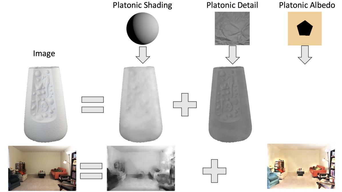
Figure 1: We learn models for platonic albedo, shading, and detail independently from platonic images. We can then combine them as shown to perform decompositions tasks. For example, we can decompose the shading and detail from the vase, or the albedo and shading of the room using the same shading model trained on platonic shading. Note that the decompositions of shading for the vase captures the generalized cylindrical shape, and the shading of the corners of the room are noticably darker. Figures best viewed in high resolution in color.

Unfortunately, collecting images and decomposing them into ground truth albedo, shading, and shading detail appears to be impossible. It is comparably easier to collect datasets which represent the Platonic ideals for each layer independently. For example, albedo images are piecewise constant Mondrians, shading images are realistically rendered 3D primitives, and shading detail (roughly the contribution of surface bumps) is swatches of reasonable materials (eg. stucco walls, sand, crumpled paper) that have minimal long scale shading effects. These independently trained generative models form a generative basis for images that can be combined to produce layers that explain a full image.

Using generative models for the decomposition task won’t work unless the models are capable of producing something that looks like images. This requires significant architectural innovation, since current generative models create rather small and blurry images. Our innovation is the convolutional variant of the Variational Auto Encoder (VAE) that is capable of producing high quality images. We call this variant, a conv-VAE and evaluate its representational power on images.

Contributions: 1) We describe a Convolutional Variational Auto Encoder that is capable of representing high frequency image information. 2) We author models using the conv-VAE for specific platonic phenomena which generalize to the real phenomena. 3) We decompose images into intrinsic layers even when ground truth decomposition of images into the layers cannot be constructed.

3 Background

Image Prediction using Neural Networks: Neural networks have been applied in relatively direct ways to predict various per pixel measures including colorization [44, 26], superresolution [7], intrinsic image decomposition [31], depth [10], surface normals, semantic labels [30], pixel values [38], various combinations [9, 1], and [19] introduce a generally applicable image-to-image translation tool.

Minimizing perceptual losses allows for the production of stylized images [14, 27] and textures [13, 37]. These perceptual losses can be used to train feedforward networks as in [20] and [28]. Perceptual losses can also be learned with GANs as in [8].

Generative Models for images Other recent work builds on generative models like encode-decoders, VAEs [22], or GANs [16]. VAEs have been used on images [21], faces [23, 43], inpainting [32], prediction of motion [39, 42], and room surface normals and textures [40]. GANs have been used to generate images [34] and 3D shapes [41]. When combined with VAEs, GANs can be used to learn losses [25]. The most similar work in this space to ours is [46] who use VAEs to represent an image manifold. However, our conv-VAE framework allows us to generate high resolution images directly from a VAE.

Intrinsic Image Decomposition: Splitting an image into shading and albedo components is a classical computer vision problem [24], as is explaining shading by reconstructing surface normals [18]. There is a strong tradition of obtaining intrinsic images as inference on a generative physical model. Write ${\cal I}$ for the log image, ${\cal A}$ for the log albedo image, and ${\cal S}$ for the log shading image. One then assumes that ${\cal I}={\cal A}+{\cal S}$, and seeks solutions for ${\cal A}$ and ${\cal S}$ that maximize priors. Similarly, reconstructing surface normals from shading is seen as inference on a generative physical model – one seeks a normal field ${\bf n}({\bf x})$ that explains the shading ${\cal S}$ under some rendering model [18]. Barron and Malik show that attacking these problems together yields an extremely strong method for recovering albedo and shading, as well as the best current shape reconstructions [2].

These traditions are odd. It is easily verified with current datasets (eg. [17, 3]) that ${\cal I}\neq{\cal A}+{\cal S}$ (as a result of mesostructure, glossy, and subsurface scattering phenomena). Even in constrained lab environments built to determine ground truth, it is difficult to fully separate the phenomena into the correct layers, in ground truth images from [17] the mesostructure shading bleeds into the albedo layer. Similarly, all shading models that yield tractable reconstruction methods are physically incorrect [11].

Prior to neural networks, methods for intrinsic images [15, 2, 36] used hand defined priors for the albedo and shading channels in [17]. Recent works, which use neural networks to predict intrinsic image decompositions [31, 47] directly use SINTEL [4] or IIW [3] to augment the MIT dataset because they otherwise will not have enough data. Our method, does not need ground truth decompositions because we do not train the albedo, shading, or shading detail models jointly. Instead, we train independent representations on Platonic ideals, and then combine them to form a decomposition model.

4 VAE Architecture

We will briefly describe VAEs in practice to motivate our conv-VAE. In depth theoretical discussion can be found in [22] and a nice tutorial is [6].

In essence, one can think about training a VAE as training two networks, an encoder $E(I)$ which is trained to map images $I$ to latent variables, usually called codes $z$, and a decoder $D(z)$ that is trained to map these codes to images. A variational criterion is used to ensure that (a) codes are distributed as $z\sim\mathcal{N}(0,1)$ (b) decoding a code $D(z)$, with $z=E(I)$ yields the image $I$ and (c) decoding a code near some $z=E(I)$ yields an image close to $I$.

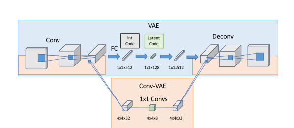
Figure 2: The difference between a VAE and convolutional VAE is entirely in the “code” layers. Notice that the dimensionality of the latent representation doesn’t change, but the size of the representation is drastically reduced because very large fully connected layers are replaced by 1x1 convolutions. Replacing the fully connected layers with convolutions can be thought of as constructing a diagonal matrix, and does not significantly impact the VAE theory.

4.1 Convolutional VAE

The basic VAE has some problems as a model for images, especially high resolution images. First, the VAE model has difficulties producing high spatial frequencies. Second, the global codes make it difficult to learn that images are shift and rotationally invariant. Third, there is no way to apply a VAE to images of varying sizes. Previous works have tried to solve these issues by generating images pixel-by-pixel, conditioning on previously seen pixels.[38]

We propose the conv-VAE for achieving these goals. Rather than creating a single global code for an image, we create a field of codes that describe local regions. This means that our latent space is a code “image” rather than a code vector as shown in figure 2. For example, on a 64x64 image, we would write a 128 bit code as a 4x4x8 code, where each “pixel” location impacts about one quarter of the output image. Since we replaced a fully connected layer that produced a 128 bit code with a convolution that produces 8 bit codes, it reduces the number of parameters in the network. However, the conv-VAE is still capable of reproducing images better because it strictly enforces locality in the latent space. This comes at the cost of independence between the dimensions of the code, which makes drawing valid codes from the latent space more difficult. However, for decomposition this is not a problem because we have other constraints.

4.2 Laplacian Conv-VAE

Training conv-VAEs to produce sharp images is still difficult because the typical reconstruction loss for $D(z)$ is $\|D(E(I))-I\|^{2}$ which does not capture the importance of high frequency edges. As such, generated images are often blurry. Techniques for improving encoder-decoder results include filtering the image with a Laplacian filter to emphasize edges [43] and discretizing the continuous color space and using a cross entropy loss [38].

We extend the Laplacian filter idea by learning a VAE for each layer of a Laplacian Pyramid. This is good for three reasons. First, predicting the high frequency layers of a Laplacian Pyramid is easy because they are often 0. Second, an L2 Loss can be applied at each layer of the Laplacian Pyramid, requiring that all frequencies of the input image are correctly captured. Third, predicting each layer with a conv-VAE explicitly places additional code capacity on the higher frequencies since they are encoded as larger images. We are not the first to apply Laplacian Pyramids in generative networks. [5] train a GAN to predict a Laplacian Pyramid. Our approach differs as we do not condition across scales and instead treat our conv-VAEs at each level as independent predictors.

4.3 Modeling Examples with VAEs

We validate conv-VAEs by comparing to conventional VAEs reproduction on images from ImageNet. Unlike previous works, which resize images to a small size, we take 64x64 pixel crops during training. This makes the assumption that images are translation invariant explicit. We compare a conv-VAE with and without the Laplacian Pyramid to two conventional VAEs. VAE-1 has roughly the same number of network parameters, and VAE-2 has roughly the same number of latent values as our conv-VAEs. Due to the fully connected layers in the conventional VAE, it is impossible to provide both at once. Details of the full parameterization is provided in table 4. We train each model for 25 epochs using Adam with an exponentially decreasing step length. Other hyperparameter details are the same as for our other experiments and are given in section 5.4

Recall that a VAE has an encoder $E(I)$ and a decoder $D(z)$. To compare representational power, we take an image patch $I$ and look at the result of encoding and then decoding it: $D(E(I))$. We do this for patches of the 200 held out images select so that they lie on interesting portion of the image, rather than the background. Quantitively on an L2 error measure on the held-out patches, VAE-1 has error .23, VAE-2 has error .18, conv-VAE has error .13, and Laplacian conv-VAE has error .11. Qualitative results, shown in figure 3 validate these findings.

Our convolutional models are also capable of modeling full ImageNet images with no additional training. We encode and decode using full images rather than patches as above. Results for the Laplacian conv-VAE on full images is shown in figure 4. We emphasize that our model only saw 64x64 patches during training, but it correctly reproduces the long-scale structure of the image.

(a) Image

(b) vae-1

(c) vae-2

(d) cvae

(e) lcvae

Figure 3: Conv-VAEs (d) and (e) always outperform traditional VAEs (b) and (c) even though (c) has as large a latent space, and the conv-VAEs have far fewer parameters. The Laplacian conv-VAE (e) is more capable of reconstructing small features of images than the conv-VAE (d). Even for relative failure cases for the method, like the last row, the conv-VAEs perform significantly better. Best viewed in color at high resolution

Figure 4: Laplacian conv-VAE trained with 64x64 patches on full images. On the left is the input image. On the right is an image created by encoding and then decoding the input image. Our model typically does a good job of handling image phenomena, though there are some mild checkerboard patterns. Best viewed in color at high resolution.

4.4 Decomposition with conv-VAE Models

We have described a method that can learn high quality representations for images. Assume that we have a generative model for log Platonic albedo and a generative model for log Platonic shading. We want to use these models to decompose an image into its component parts. We note that some albedo (resp. shading) codes are more common than others. Furthermore, when there are phenomena that can be explained by either layer (eg. cast shadows) we want to force our decomposition to choose – the layers should not have strong correlation. We would like to obtain a decomposition that (a) uses common codes for each layer (b) explains the image and (c) produces decorrelated layers.

The conv-VAE models are composed of $E_{a}(\cdot)$ and $D_{a}(\cdot)$ for the albedo encoder and decoder. Similarly, $E_{s}(\cdot)$ and $D_{s}(\cdot)$ describe the VAE for shading. For the Laplacian conv-VAE, the encoder and decoder produce a set of code images and a Laplacian decomposition respectively. We build a probabilistic model of common codes per code “pixel” for albedo and shading. First, we encode ground truth patches to recover code images. For the Laplacian conv-VAE, we recover the set of code “images”, and concatenate the codes, resizing the smaller “images” to the size of the largest “image”. We then treat each pixel as an iid draw from a distribution and fit a probability density model to the set. In practice we use a Gaussian model with a spherical covariance. Let the probability models for albedo and shading be $P_{a}(z)$ and $P_{s}(z)$. Let $z^{a}_{i}$ be the $i$th pixel of the albedo code, (resp $z^{s}_{i}$). We write the full code loss as a negative log likelihood $P(z^{a},z^{s})=-1/N\sum_{i}\log(P_{a}(z^{a}_{i}))+\log(P_{s}(z^{s}_{i}))$.

As is traditional in intrinsic images, we enforce the image be explained by the codes by minimizing the residual $\mathcal{R}(z^{s},z^{a},I)=\|\log(I)-D_{s}(z^{s})-D_{a}(z^{a})\|^{2}$.

To decorrelate the layers, we introduce a term which is meant to force the decomposition to “make up its mind” about where a signal should live. We define an upper bound on the correlation with the Frobenius norm of the 3x3 covariance matrix of the spatially corresponding pixel values in the albedo and shading. This correlation measure is attractive because it is simple and can be applied patch-wise, at varying scales, and across Laplacian layers. Let $\text{cov}(\cdot,\cdot)$ be the operation that computes the covariance matrix by centering two signals, and then taking the mean of the outer products. Let $P$ be the number of patches and $L$ the number of Laplacian layers. Let $A^{(l)}_{p}$ be the $p$th patch in the $l$th Laplacian layer of the albedo prediction. The correlation is $\text{corr}(A,S)=\frac{1}{L\cdot P}\sum_{l}\sum_{p}\|\text{cov}(A^{(l)}_{p},S^{(l)}_{p})\|_{F}$

Our full decomposition equation is

$$\operatorname*{arg\,min}_{z^{a},z^{s}} \mathcal{R}(z^{s},z^{a},I)$$ (1)

$$-\lambda_{p}P(z^{a},z^{s})$$

$$+\lambda_{c}\text{corr}(D_{s}(z_{s}),D_{a}(z_{a}))$$

5 Authored Training Data and Models

Filter	Layer
[HTML]BBDAFF	128x128x3	64x64x3	32x32x3	16x16x3
5x5	64x64x64	32x32x64	16x16x64	8x8x64
5x5	32x32x64	16x16x64	8x8x64	4x4x64
3x3	32x32x64	16x16x64	8x8x64	4x4x64
4x4	29x29x64	13x13x64	5x5x64	1x1x64
[HTML]B8D8A4 1x1	29x29x4	13x13x4	5x5x4	1x1x4

Table 1: The VAE architecture we use for all of our authored models is a Laplacian conv-VAE with 4 Laplacian layers, and a code size of 4 per code “pixel”. As in table 4, we show only the encoder portion, as the decoder is the reverse. For a 128x128 image, this compresses to about 8% of the original image size. In the limit as image size increases, the compression rate is about 11%.

(a) Platonic albedo is two color Mondrian images.

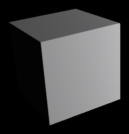
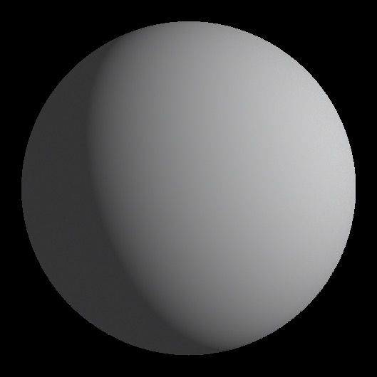
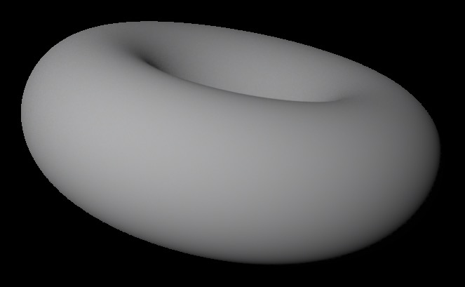
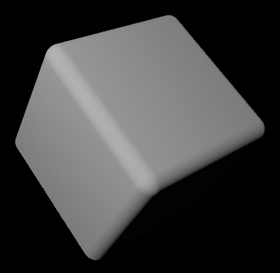
(b) Platonic shading is rendered primitive shapes under varying lighting conditions.

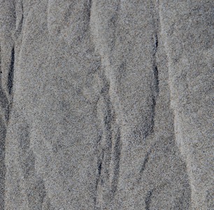
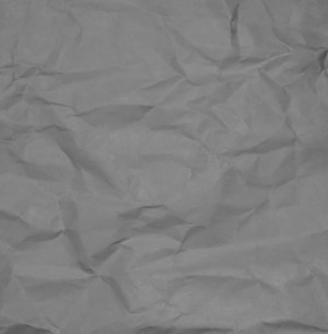
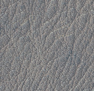
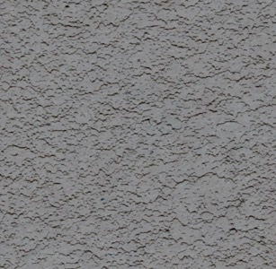
(c) Platonic shading detail is caused by small bumps on an otherwise flat smooth surface under uniform lighting.

Figure 5: Example Platonic training data images are used to train VAE models. Notice that the representation each captures is unique.

5.1 Albedo

Platonic albedo, figure 5(a), is piecewise constant. We create a set of 2-color Mondrian images, where a polygon at the center has a different color than the rest of the image. The colors for these are drawn from the palette of colors from the 10-train set of MIT images. We generate 500 Mondrian images of size 150x150 to allow for 128x128 crops that are shifted or rotated.

5.2 Shading

Platonic shading, figure 5(b), is the effect of light on a simple smooth surface. We generate platonic shadings by rendering 3D primitives with no surface color using LuxRender. We use a directional light source which rotates about the the object with a fixed camera view. We either provide a fill light where dark pixels get about 10% of pure white, or a weak fill light where dark pixels get about 1% of pure white. The weak fill light matches the lighting conditions found in MIT, while the stronger fill light is a good proxy for more typical lighting, where diffuse components are quite large. There are 70 images, cropped to the bounding box of the rendered object so that the images are about 500x500 pixels. During training, we take 128x128 crops from these, such that the crops lie mostly inside of the masked object.

5.3 Shading Detail

Platonic shading detail, figure 5(c) is the effect from small bumps on a flat smooth surface under uniform lighting. We collect swatches of materials from the Internet including sand which has wavy texture, stucco which has repetitive bumps, and creased paper which varies between the two. These images are similar to those used in video games for texturing. These swatches are mostly planar and have minimal long-scale shading effects and almost no albedo effects. We remove contributions of shading and center the images at .5 by fitting a linear shading gradient to the image. We also crop to $[0,1]$, to guarantee existence of the log image. Our dataset consists of 45 images of about 300x300 pixels.

5.4 Laplacian conv-VAE Training Details

Our VAE model’s architecture is described in table 1. We use a 4-layer Laplacian decomposition, but it is otherwise the same as the Laplacian conv-VAE used on ImageNet. We train the model to encode and decode log versions of the images so that they can be used directly for intrinsic image decomposition, where it is common to write $\log(I)=\log(A)+\log(S)$. This also means that we do not use a sigmoid activation layer for the final output layer. We use the Adam optimizer with an exponentially decaying learning rate starting at .001 decaying every 500 iterations by .9. For $t$, the iteration and $\sigma(\cdot)$ the sigmoid function, our KL divergence terms weight is $20\sigma(.02\cdot t-.5)$. The image residual loss is weighted by $1000$. An image prior, the L1 of image gradients, is weighted by $.1$.

6 Experimental Results

We emphasize that all results are obtained with the same models of Platonic albedo (A), shading (S), and shading detail (D). Different decompositions are obtained by using different combinations of models (i.e. A,S; S,D; A,S,D; etc).

6.1 Albedo and Shading Decomposition

We decompose images into Albedo and shading using our authored models. We use the 10-image MIT train set to perform a cursory search of parameters for weighting the probability models, correlation, and image reconstruction term. We present quantitative results in table 2 on the 10-MIT test dataset for real color images. We use the typical scaled MSE measures from [2]. Our qualitative results are shown in figure 6. We also present quantitative results on WHDR on IIW from [3] using the same model in table 3. Since our model is not trained to perform decompositions which maximize the WHDR measure, we search for an optimal threshold using the first 100 images from IIW. We compare to decompositions from [3] in figure 7.

We set parameters as follows: .0001 for the probability models, 10k for the correlation, and 100 for the image reconstruction term. While the loss we are optimizing is drastically nonconvex, a trick that we found helpful for determining weights was to initialize the model near the ground truth decomposition, and look for weights that were stable at that point. Another important trick was finding a good initialization. For albedo and shading, we initialize shading at a smoothed version of the image, and albedo to the residual.

	S-MSE	R-MSE	RS-MSE
Naive Baseline	.0577	.0455	.0354
Retinex	.0204	.0186	.0163
Gehler et. al. [15]	.0106	.0101	.0131
Barron et. al. [2]	.0064	.0098	.0125
Ours S, A	.0134	.0175	.0253
Ours S+Sd, A	.0131	.0160	.0250

Table 2: We compare to intrinsic image techniques on the MIT dataset. Similar to the method presented in [3] our method beats Retinex. We achieve this result without architecting a solution directly on the decomposition of MIT images as other prior works have. We perform relatively poorly on RS-MSE because it heavily penalizes small wiggles in constant value regions.

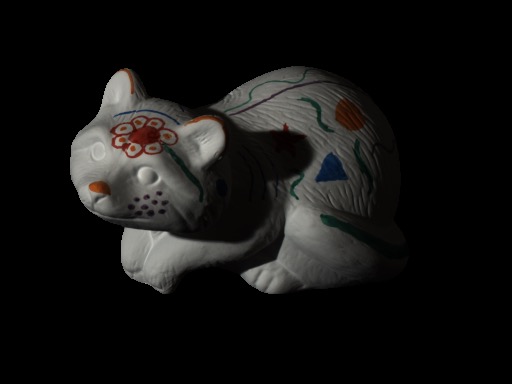
(a) Input Image

(b) GT Albedo

(c) GT Shading

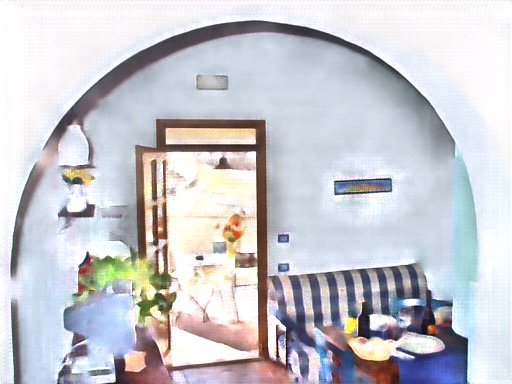
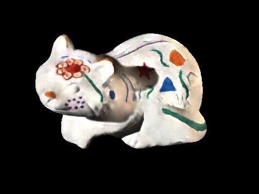
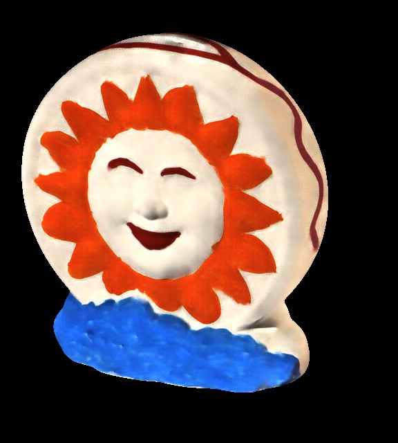
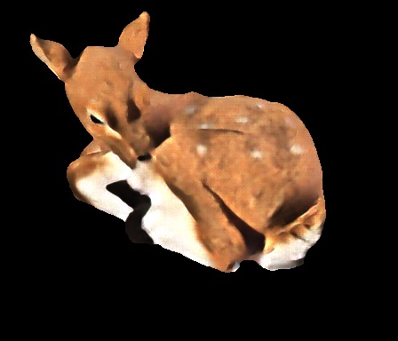
(d) Pred Albedo

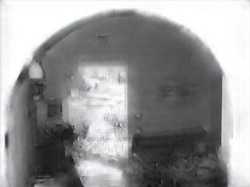
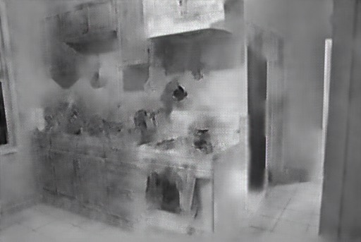
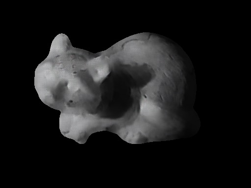
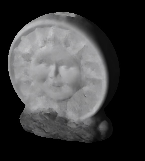
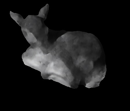
(e) Pred Shading

Figure 6: Our Intrinsic image decomposition results on MIT test data (bottom 3) and IIW images (top 2) are qualitatively good even though our model was never trained to do decomposition on images. Our model produces albedo (resp. shading) fields with a strong similarity to the ideal (eg. constant patches of color). This is pronounced compared even to the MIT ground truth. For example, is the roughness at the base of the sun in gt really an albedo effect? Best viewed in high resolution in color. All images produced using the same platonic models, but in different combinations (A,S here).

(a) Input Image

(b) Our Albedo

(c) Our Shading

(d) Bell et al. Albedo

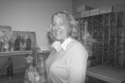
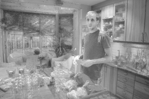
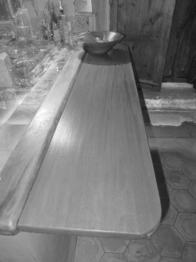
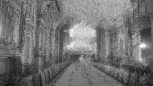
(e) Bell et al. Shading

Figure 7: We compare the best results (top 5 rows, WHDR = 0.0%) from Bell et al. to our results on the same images. We also compare to good results (bottom 3 rows, WHDR = 6.5%). We did not pick any results based on our WHDR scores. Notice that our results are occasionally locally better. For example, in the third row, look at the shadow from the bowl, in the last row look at the bright light on the center of the floor.

Algorithm	WHDR
Bell et al. [3]	21.1
Zhao et al. [45]	23.7
Garces et al. [12]	25.9
Retinex (gray) [17]	27.3
Retinex (color)	27.4
Ours (Linear .25)	27.9
Shen et al. [35]	32.4
Ours (Linear .1)	34.9
Baseline (const R)	36.6
Ours (sRGB .1)	47.3
Baseline (const S)	51.6

Table 3: Results on IIW. All other algorithms were tuned for WHDR with a threshold of .1, ours was not. As such, we search for an optimal value for the threshold (.25) on the first 100 images from IIW, and report results. Other numbers from [3].

(a) Input Image

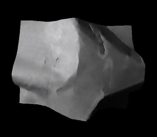
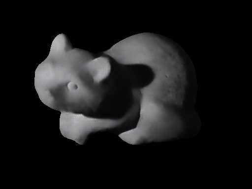
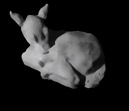
(b) Shading

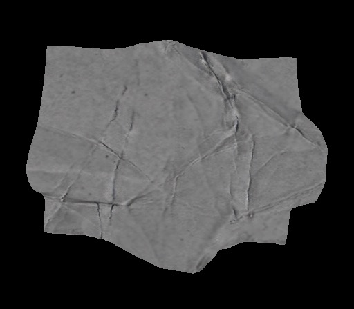
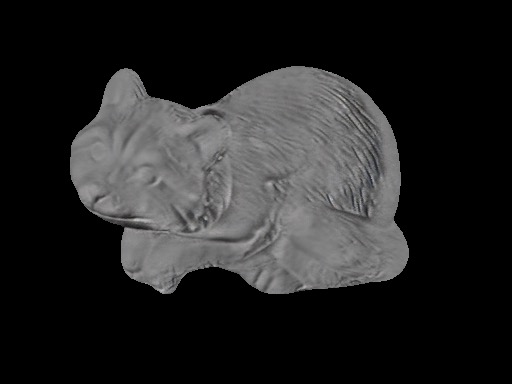
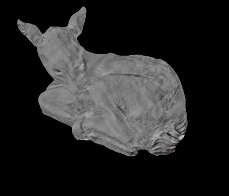
(c) Shading Detail

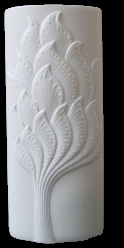
(d) Input Image

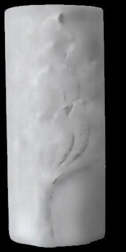
(e) Shading

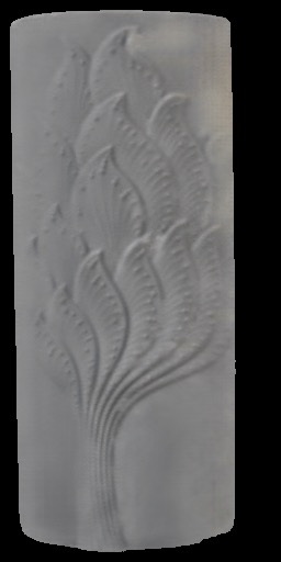
(f) Shading Detail

Figure 8: Decomposition of shading into shading from shape and shading detail. Notice that the shading detail recovers texture even in the dark shading on the raccoon’s back. Notice also that we can decompose real images outside the MIT dataset with the same model. All images produced using the same platonic models, but in different combinations (here S,D).

6.2 Shading and Shading Detail

Another cool application is decomposing shading into shading and shading detail. It is especially interesting because, unlike albedo and shading there is no easy way to capture images of an object with and without shading detail. As such, there are no ground truth decompositions of images into shading and shading detail. However, the effect of the decomposition is obvious. The shading image captures the global shape of an object, while the shading detail captures the texture or “feel” of the object. It is also worth noting that it works well on MIT even when the detail is in deep shadow. It is also general, and can decompose images of white generalized cylinders (vases). We show both in figure 8. Additional results on vases can be found in figure 15, all results on MIT can be found in the appendix.

The details of our model are similar to the albedo and shading decomposition. We use .0001 for the probability weights, 10k for the correlation, and 100 for the image reconstruction term. We initialize the shading image to be a smoothed version of the input image on MIT (the image for vases), and the material to be a constant image.

6.3 Albedo, Shading, and Shading Detail

Finally, we can generalize our model to decompose images into three phenomena at once. We evaluate how well this works on MIT by composing shading and shading detail to form a single shading image. As we can see in table 2, incorporating these three channels improves quantitative performance, since we accurately determine that shading detail should be attributed to shading. We show output images in figure 9 and additional results can be found in the appendix.

We use parameters .0001 for the probability models, 10k for the correlation, and we have to increase the image reconstruction term to 10000 because the correlation model contains the contribution from all pairs.

(a) Input Image

(b) GT Albedo

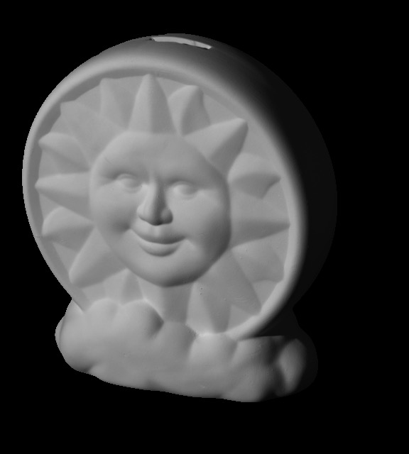
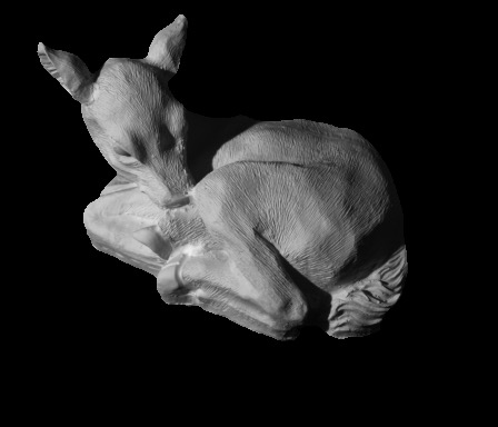
(c) GT Shading

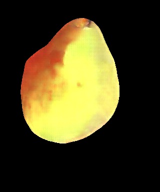
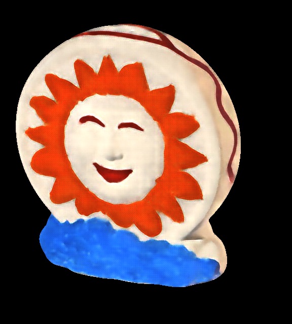
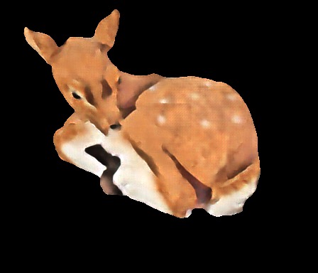
(d) Pred Albedo

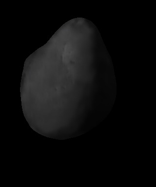
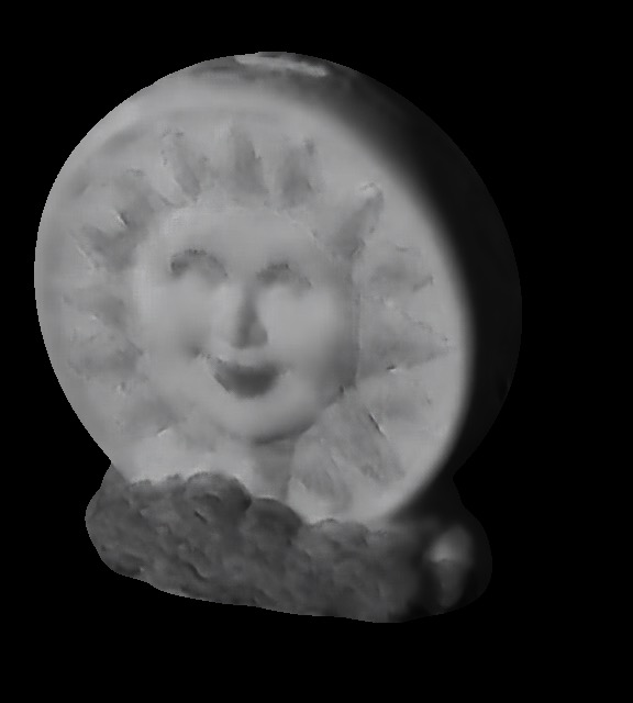
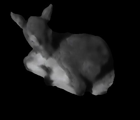
(e) Pred Shading

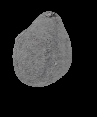
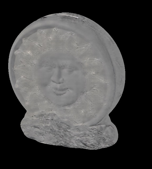
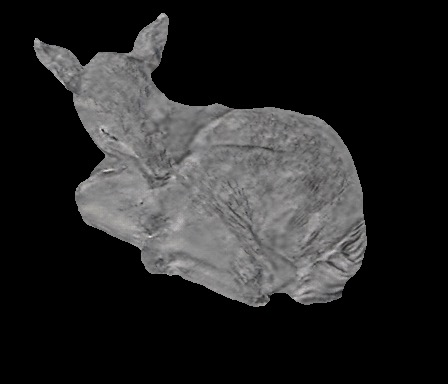
(f) Shading Detail

Figure 9: Our model can extend to decompose three layers: shading, detail, and albedo. The outputs are qualitatively very good, especially the albedos which are generally constant and the shading details which take small bumpy details. Best viewed in high resolution in color. All images are produced using the same platonic models, but in different combinations (here A,S,D).

7 Discussion

We have demonstrated a method for decomposing images into component channels using authored models to determine the channels. We represent albedo (resp. shading, shading detail) by the signals that a learned generative model is capable of producing. We obtain strong performance, because our models use a novel pyramid conv-VAE architecture that can reproduce fine image detail. A particular attraction of our approach is that it applies in the absence of canonical or ground-truth decompositions of images; instead, one provides platonic ideals for the layers envisaged. In the future we want to explore the tradeoffs between bias and variance in authoring the models, either in adjustment of the conv-VAE hyperparameters, or choosing different sets of images as our platonic examples. We plan to investigate decomposing images into different layers, possibly even layers that are not compositionally related to the image. Introducing other losses on the produced images could also lead to improvements in decomposition, for example, a bias for specific colors in albedos. Conv-VAE’s involve a compromise; it is hard to sample a conv-VAE, because codes at each pixel are not independent. In future, we will investigate sampling conv-VAE’s to produce a fully generative model that can produce high resolution images.

Appendix A VAE Architectures

Our VAE and conv-VAE architectures used for comparison are described in detail in table 4.

Appendix B Comparison to Isola et. al.

Image-to-Image translation [19], a concurrent paper with ours, demonstrates how to predict images from other images. We evaluate image-to-image translation on MIT and IIW qualitatively in figure 11. We find that the model is capable of learning MIT albedo prediction when trained on MIT, but the model does not generalize to IIW.

We also train an image-to-image prediction model on our authored data by creating shaded Mondrian images. These are formed by compositing Mondrians and shading images. As shown in figure 10, the model can predict the Mondrian albedos, but the model does not generalize to predicting albedos on MIT or IIW (figure 11).

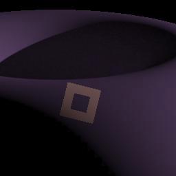
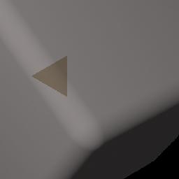
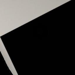
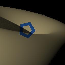
(a) input image

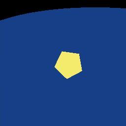
(b) GT Albedo

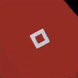
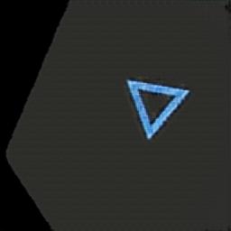
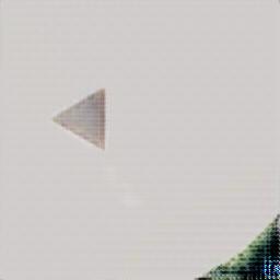
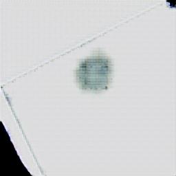
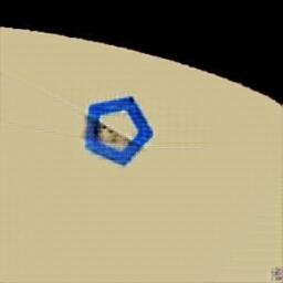
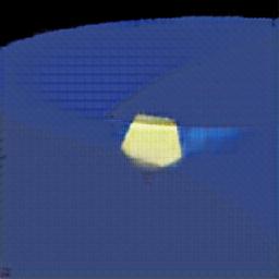
(c) Prediction

Figure 10: Using Image-to-Image [19] to learn to predict Mondrian albedos during training works well. However, as shown in figure 11, this model does not generalize well to real images.

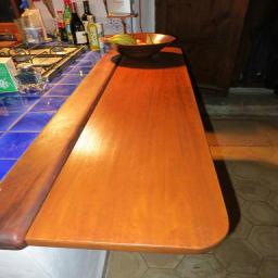
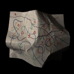
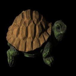
(a) Input Image

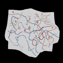
(b) Albedo GT

(c) Albedo Pred

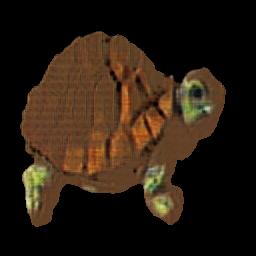
(d) Patch Pred

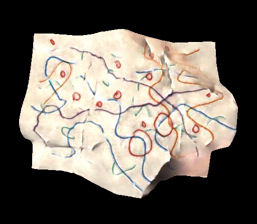
(e) Ours

Figure 11: While Isola et. al. [19] performs well on MIT when trained with MIT (rows 3 and 4, column 3). However, the model does not generalize well to IIW as small details on the wine rack or table are eliminated (rows 1 and 2). When trained on images composed from Mondrian and shading images, the results are poor on both IIW and MIT as colors bleed across boundaries (column d). Our result is shown in column e for comparison.

	VAE-1		VAE-2		conv-VAE		Laplacian conv-VAE
	Filter	Layer	Filter	Layer	Filter	Layer	Filter	Layer
[HTML]BBDAFF Image		64x64x3		64x64x3		64x64x3		64x64x3	32x32x3	16x16x3
	5x5	32x32x64	5x5	32x32x64	5x5	32x32x64	5x5	32x32x64	16x16x64	8x8x64
	5x5	16x16x128	5x5	16x16x128	5x5	16x16x128	5x5	16x16x64	8x8x64	4x4x64
	3x3	16x16x128	3x3	16x16x128	3x3	16x16x128	3x3	16x16x64	8x8x64	4x4x64
	fc	128	fc	4096	4x4	13x13x20	4x4	13x13x16	5x5x16	1x1x16
[HTML]B8D8A4 Code	fc	32	fc	832	1x1	13x13x8	1x1	13x13x4	5x5x4	1x1x4

Table 4: Architecture for the encoding portion of the VAE, conv-VAE, and Laplacian conv-VAE for comparison. The decoding portion is the same in reverse. For a fair comparison, we compare two VAEs. VAE-1 has roughly the same number of parameters as the conv-VAE, while VAE-2 has the same code dimensionality, but drastically more parameters. When converting from Laplacian conv-VAE to conv-VAE we matched the intermediate sizes when possible, but always rounded up when necessary.

Appendix C Albedo Shading on MIT

All decompositions for MIT test are shown in figure 12.

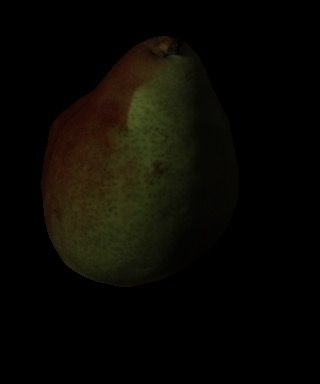
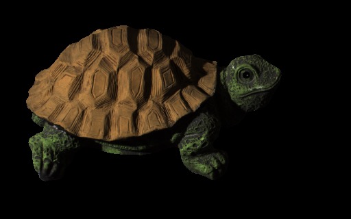
(a) Input Image

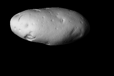
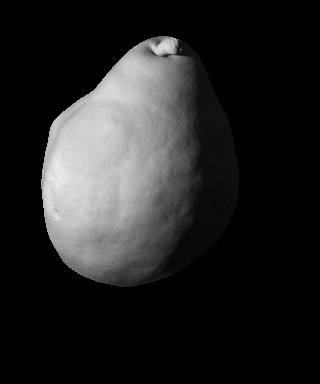
(b) Shading GT

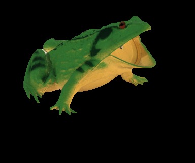
(c) Albedo GT

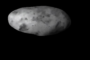
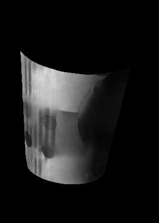
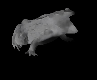
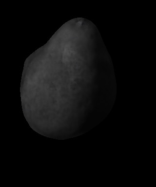
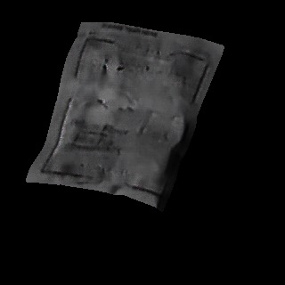
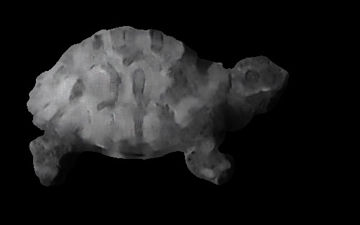
(d) Shading

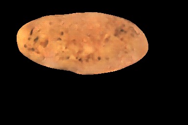
(e) Albedo

Figure 12: Albedo and Shading decompositions on all images from MIT Test for our method.

Appendix D Albedo, Shading, and Shading Detail on MIT

All decompositions for MIT test are shown in figure 13.

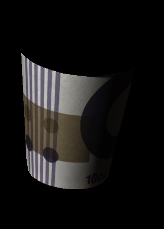
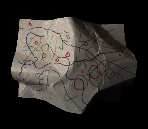
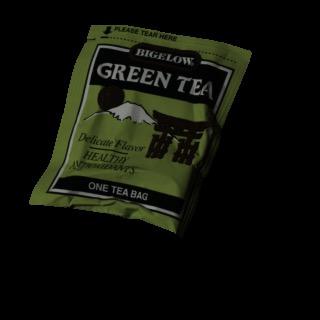
(a) Input Image

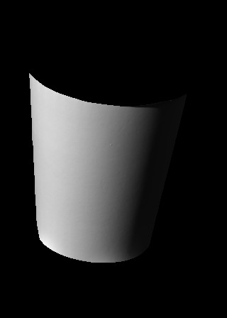
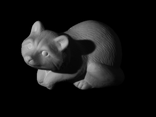
(b) Shading GT

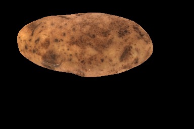
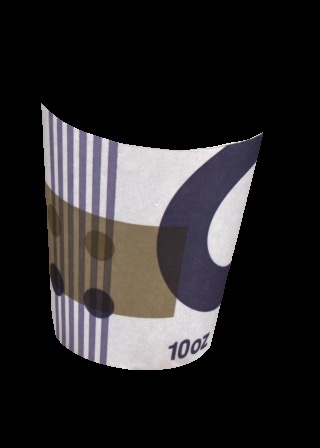
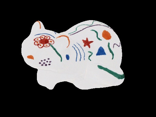
(c) Albedo GT

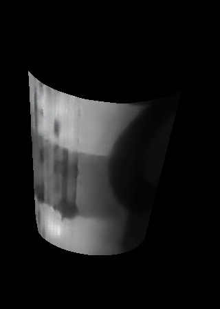
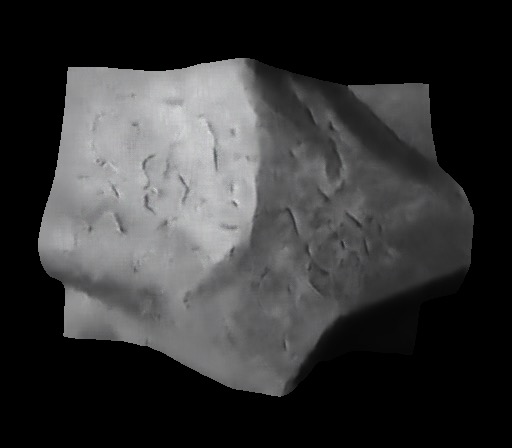
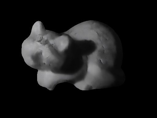
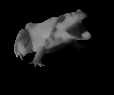
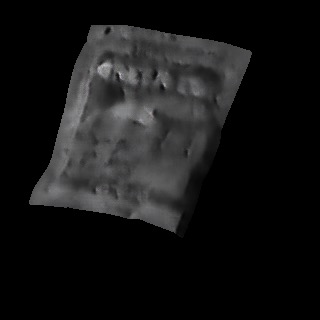
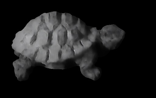
(d) Shading

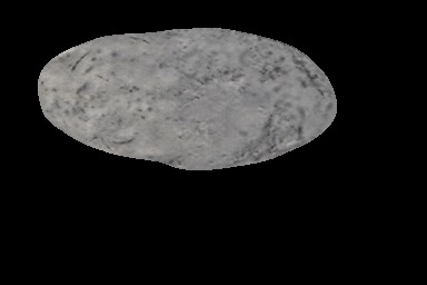
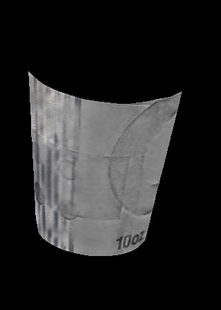
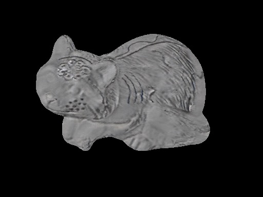
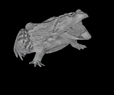
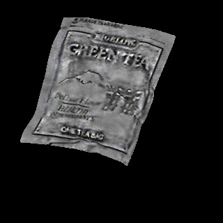
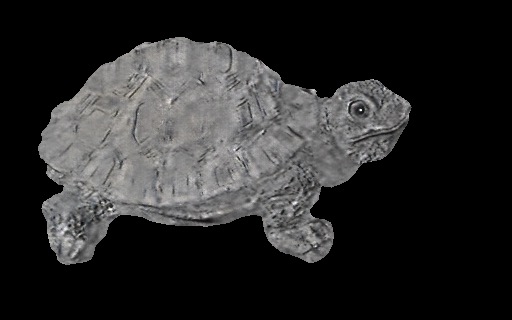
(e) Material

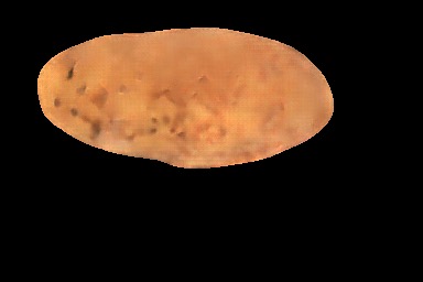
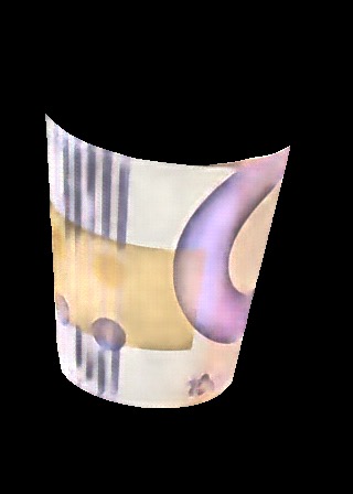
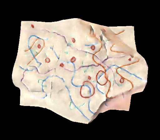
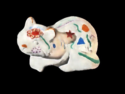
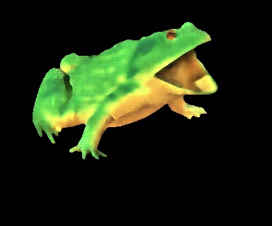
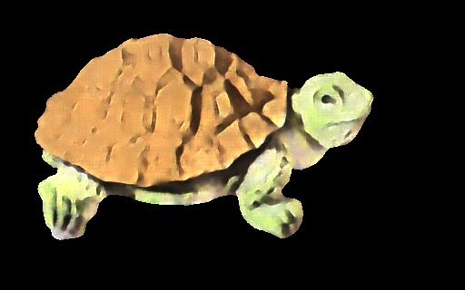
(f) Albedo

Figure 13: Albedo, Shading, and Shading Detail decompositions on all images from MIT Test for our method.

Appendix E Shading Shading Detail on MIT

All decompositions for MIT, test and train, are shown in figure 14.

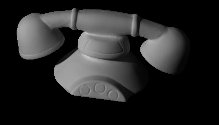
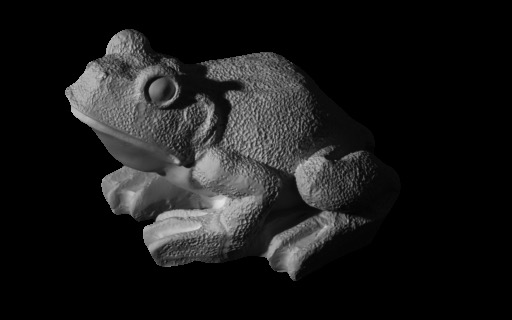
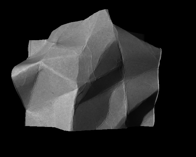
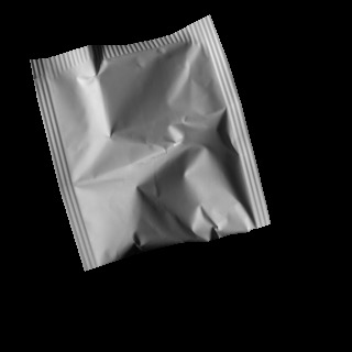
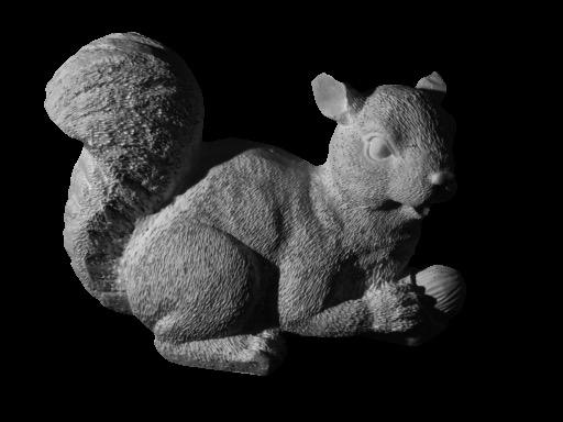
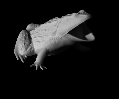
(a) Input Image

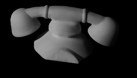
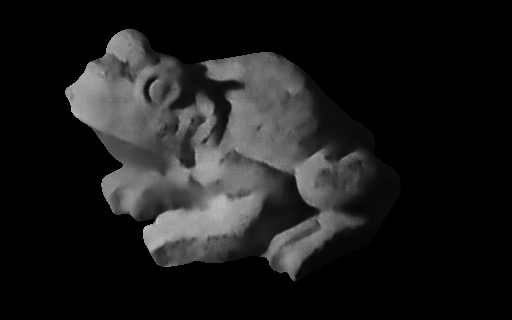
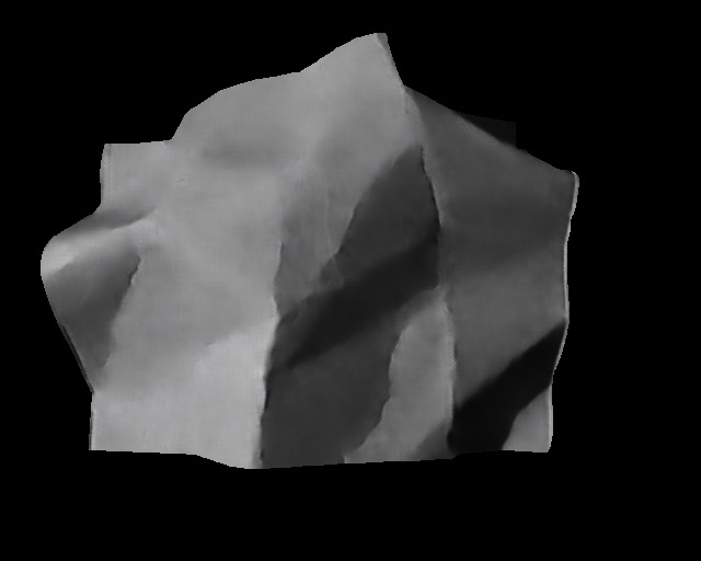
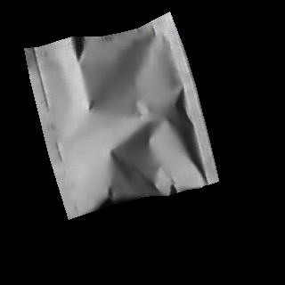
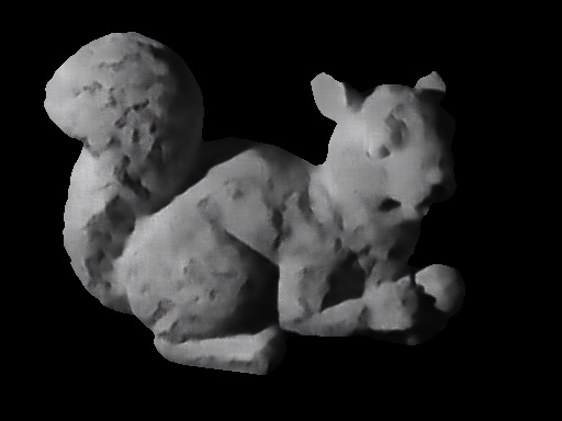
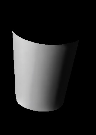
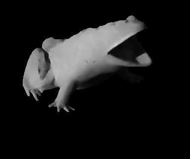
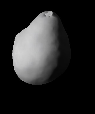
(b) Shading

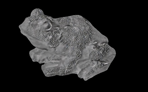
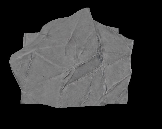
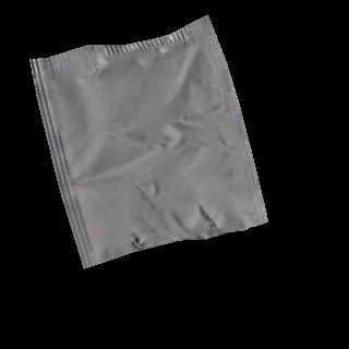
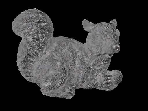
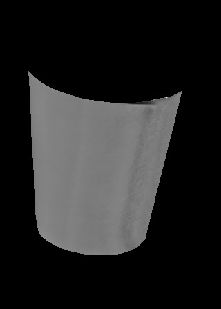
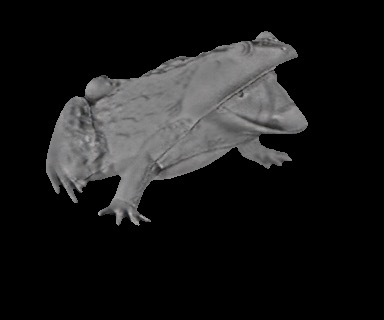
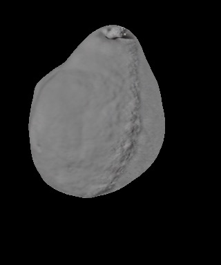
(c) Detail

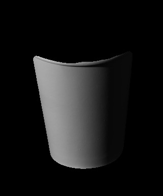
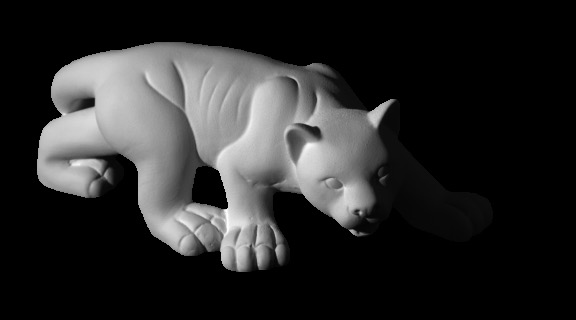
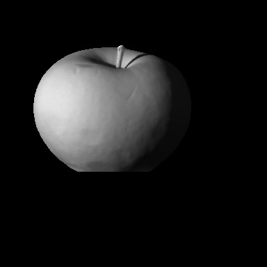
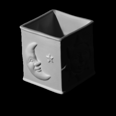
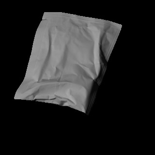
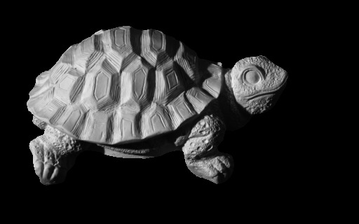
(d) Input Image

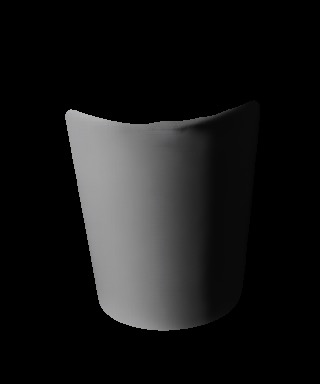
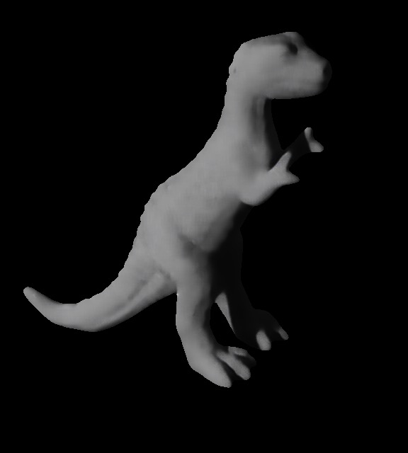
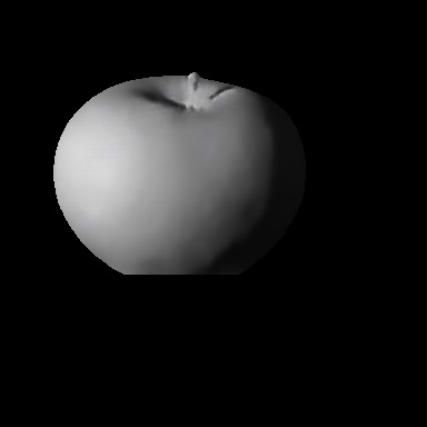
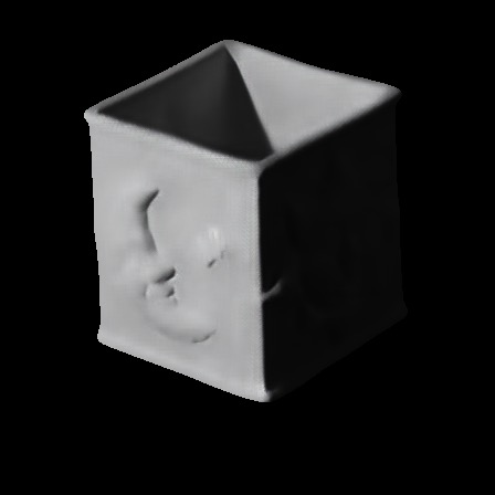
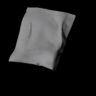
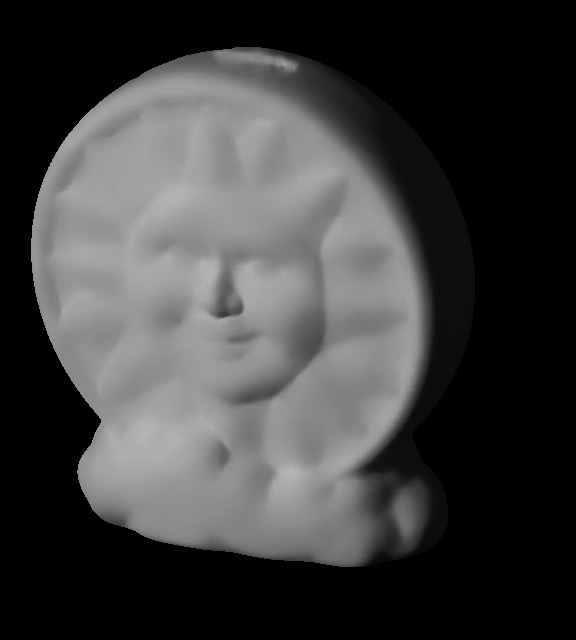
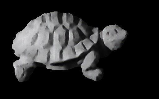
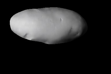
(e) Shading

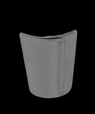
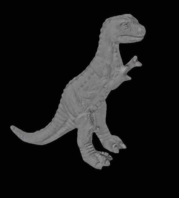
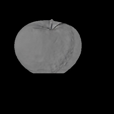
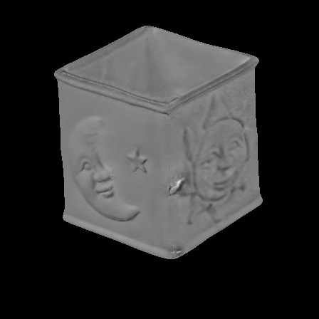
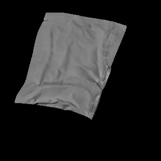
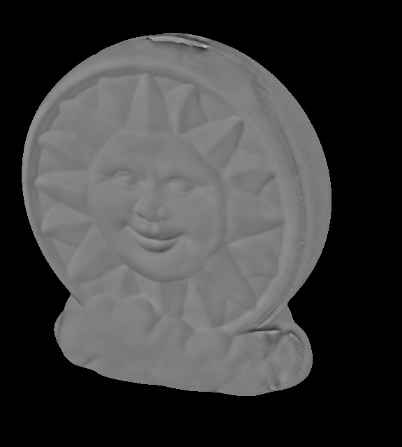
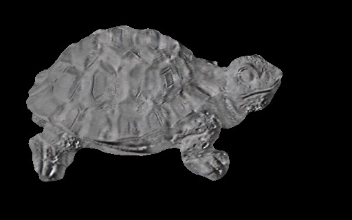
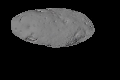
(f) Detail

Figure 14: Shading and Shading Detail decompositions on MIT from our method.

Appendix F Shading Shading Detail on Vases

Decompositions of vases into shading and shading detail are shown in figure 15

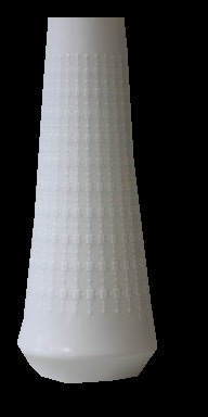
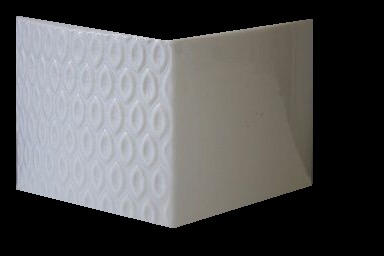
(a) Input Image

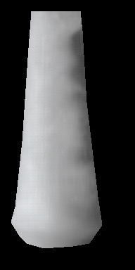
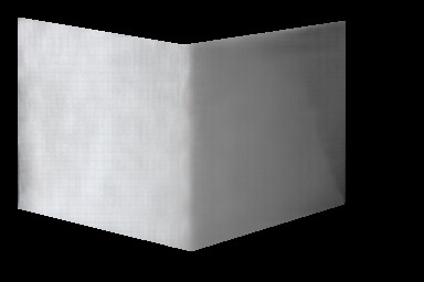
(b) Shading

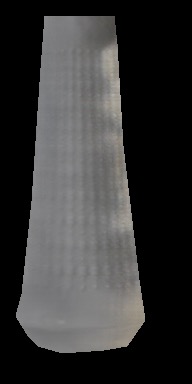
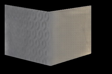
(c) Shading Detail

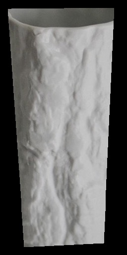
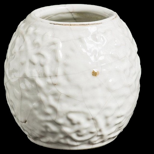
(d) Input Image

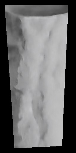
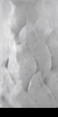
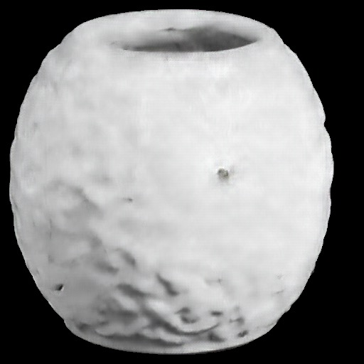
(e) Shading

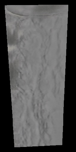
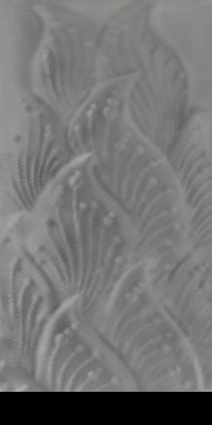
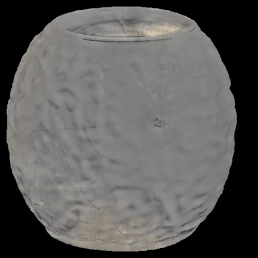
(f) Shading Detail

Figure 15: Shading and Shading Detail decompositions on vases for our method.

References

- [1] A. Bansal, X. Chen, B. Russell, A. Gupta, and D. Ramanan. PixelNet: Towards a General Pixel-level Architecture. arXiv.org, Sept. 2016.
- [2] J. T. Barron and J. Malik. Shape, Illumination, and Reflectance from Shading. PAMI, 37(8):1670–1687, 2015.
- [3] S. Bell, K. Bala, and N. Snavely. Intrinsic images in the wild. ACM Trans. Graph., 33(4):159:1–159:12, July 2014.
- [4] D. J. Butler, J. Wulff, G. B. Stanley, and M. J. Black. A naturalistic open source movie for optical flow evaluation. In A. Fitzgibbon et al. (Eds.), editor, European Conf. on Computer Vision (ECCV), Part IV, LNCS 7577, pages 611–625. Springer-Verlag, Oct. 2012.
- [5] E. L. Denton, S. Chintala, a. szlam, and R. Fergus. Deep Generative Image Models using a Laplacian Pyramid of Adversarial Networks. In NIPS, pages 1486–1494, 2015.
- [6] C. Doersch. Tutorial on Variational Autoencoders. Technical report, June 2016.
- [7] C. Dong, C. C. Loy, K. He, and X. Tang. Image Super-Resolution Using Deep Convolutional Networks. Pattern Analysis and Machine Intelligence, 38(2):295–307, 2016.
- [8] A. Dosovitskiy and T. Brox. Generating Images with Perceptual Similarity Metrics based on Deep Networks. arXiv.org, Feb. 2016.
- [9] D. Eigen and R. Fergus. Predicting Depth, Surface Normals and Semantic Labels with a Common Multi-scale Convolutional Architecture. In International Conference on Computer Vision, pages 2650–2658. IEEE, 2015.
- [10] D. Eigen, C. Puhrsch, and R. Fergus. Depth Map Prediction from a Single Image using a Multi-Scale Deep Network. In NIPS, 2014.
- [11] D. Forsyth and A. Zisserman. Mutual illumination. In CVPR ’89: IEEE Computer Society Conference on Computer Vision and Pattern Recognition, pages 466–473. IEEE, 1989.
- [12] E. Garces, A. Munoz, J. Lopez-Moreno, and D. Gutierrez. Intrinsic images by clustering. In Computer graphics forum, pages 1415–1424. Wiley Online Library, 2012.
- [13] L. A. Gatys, A. S. Ecker, and M. Bethge. Texture Synthesis Using Convolutional Neural Networks. arXiv.org, May 2015.
- [14] L. A. Gatys, A. S. Ecker, and M. Bethge. Image Style Transfer Using Convolutional Neural Networks. In Computer Vision and Pattern Recognition, pages 2414–2423, 2016.
- [15] P. V. Gehler, C. Rother, M. Kiefel, L. Zhang, and B. Scholkopf. Recovering Intrinsic Images with a Global Sparsity Prior on Reflectance. In NIPS, pages 765–773, 2011.
- [16] I. Goodfellow, J. Pouget-Abadie, and M. Mirza. Generative adversarial nets. In NIPS, 2014.
- [17] R. Grosse, M. K. Johnson, E. H. Adelson, and W. T. Freeman. Ground-truth dataset and baseline evaluations for intrinsic image algorithms. In International Conference on Computer Vision, pages 2335–2342, 2009.
- [18] B. K. Horn. Shape from shading: A method for obtaining the shape of a smooth opaque object from one view. 1970.
- [19] P. Isola, J.-Y. Zhu, T. Zhou, and A. A. Efros. Image-to-Image Translation with Conditional Adversarial Networks. arXiv.org, Nov. 2016.
- [20] J. Johnson, A. Alahi, and L. Fei-Fei. Perceptual Losses for Real-Time Style Transfer and Super-Resolution. arXiv.org, Mar. 2016.
- [21] D. P. Kingma, T. Salimans, and M. Welling. Improving Variational Inference with Inverse Autoregressive Flow. arXiv.org, June 2016.
- [22] D. P. Kingma and M. Welling. Auto-encoding variational bayes. In ICLR, 2014.
- [23] T. D. Kulkarni, W. F. Whitney, P. Kohli, and J. B. Tenenbaum. Deep Convolutional Inverse Graphics Network. In NIPS, pages 2539–2547, 2015.
- [24] E. Land and J. J. Mccann. Lightness and retinex theory. J. Opt. Soc. Am., 61(1):1–11, Jan 1971.
- [25] A. B. L. Larsen, S. K. Sønderby, H. Larochelle, and O. Winther. Autoencoding beyond pixels using a learned similarity metric. In International Conference on Machine Learning, 2016.
- [26] G. Larsson, M. Maire, and G. Shakhnarovich. Learning Representations for Automatic Colorization. arXiv.org, Mar. 2016.
- [27] C. Li and M. Wand. Combining Markov Random Fields and Convolutional Neural Networks for Image Synthesis. In Computer Vision and Pattern Recognition, 2016.
- [28] C. Li and M. Wand. Precomputed Real-Time Texture Synthesis with Markovian Generative Adversarial Networks. ECCV, 2016.
- [29] Z. Liao, J. Rock, Y. Wang, and D. Forsyth. Non-parametric filtering for geometric detail extraction and material representation. In 2013 IEEE Conference on Computer Vision and Pattern Recognition, pages 963–970, Los Alamitos, CA, USA, 2013. IEEE Computer Society.
- [30] J. Long, E. Shelhamer, and T. Darrell. Fully Convolutional Networks for Semantic Segmentation. In Computer Vision and Pattern Recognition, pages 3431–3440. IEEE, 2015.
- [31] T. Narihira, M. Maire, and S. X. Yu. Direct Intrinsics: Learning Albedo-Shading Decomposition by Convolutional Regression. In International Conference on Computer Vision, Dec. 2015.
- [32] D. Pathak, P. Krähenbühl, J. Donahue, T. Darrell, and A. A. Efros. Context Encoders: Feature Learning by Inpainting. arXiv.org, Apr. 2016.
- [33] R. Ramamoorthi and P. Hanrahan. An efficient representation for irradiance environment maps. In ACM SIGGRAPH, 2001.
- [34] T. Salimans, I. J. Goodfellow, W. Zaremba, V. Cheung, A. Radford, and X. Chen. Improved Techniques for Training GANs. arXiv.org, June 2016.
- [35] J. Shen, X. Yang, Y. Jia, and X. Li. Intrinsic images using optimization. In Computer Vision and Pattern Recognition (CVPR), 2011 IEEE Conference on, pages 3481–3487. IEEE, 2011.
- [36] L. Shen and C. Yeo. Intrinsic images decomposition using a local and global sparse representation of reflectance. CVPR, 2011.
- [37] I. Ustyuzhaninov, W. Brendel, L. A. Gatys, and M. Bethge. Texture Synthesis Using Shallow Convolutional Networks with Random Filters. arXiv.org, May 2016.
- [38] A. van den Oord, N. Kalchbrenner, and K. Kavukcuoglu. Pixel Recurrent Neural Networks. ICML, 2016.
- [39] J. Walker, C. Doersch, A. Gupta, and M. Hebert. An Uncertain Future: Forecasting from Static Images using Variational Autoencoders. arXiv.org, June 2016.
- [40] X. Wang and A. Gupta. Generative Image Modeling using Style and Structure Adversarial Networks. arXiv.org, Mar. 2016.
- [41] J. Wu, C. Zhang, T. Xue, W. T. Freeman, and J. B. Tenenbaum. Learning a Probabilistic Latent Space of Object Shapes via 3D Generative-Adversarial Modeling. In NIPS, Oct. 2016.
- [42] T. Xue, J. Wu, K. L. Bouman, and W. T. Freeman. Visual Dynamics: Probabilistic Future Frame Synthesis via Cross Convolutional Networks. In NIPS, July 2016.
- [43] X. Yan, J. Yang, K. Sohn, and H. Lee. Attribute2Image - Conditional Image Generation from Visual Attributes. ECCV, 2016.
- [44] R. Zhang, P. Isola, and A. A. Efros. Colorful Image Colorization. In European Conference on Computer Vision, Mar. 2016.
- [45] Q. Zhao, P. Tan, Q. Dai, L. Shen, E. Wu, and S. Lin. A closed-form solution to retinex with nonlocal texture constraints. IEEE transactions on pattern analysis and machine intelligence, 34(7):1437–1444, 2012.
- [46] J.-Y. Zhu, P. Krähenbühl, E. Shechtman, and A. A. Efros. Generative Visual Manipulation on the Natural Image Manifold. In European Conference on Computer Vision, Sept. 2016.
- [47] D. Zoran, P. Isola, D. Krishnan, and W. T. Freeman. Learning Ordinal Relationships for Mid-Level Vision. In International Conference on Computer Vision, pages 388–396. IEEE, 2015.