ArtTrack: Articulated Multi-person Tracking in the Wild

Abstract

In this paper we propose an approach for articulated tracking of multiple people in unconstrained videos. Our starting point is a model that resembles existing architectures for single-frame pose estimation but is substantially faster. We achieve this in two ways: (1) by simplifying and sparsifying the body-part relationship graph and leveraging recent methods for faster inference, and (2) by offloading a substantial share of computation onto a feed-forward convolutional architecture that is able to detect and associate body joints of the same person even in clutter. We use this model to generate proposals for body joint locations and formulate articulated tracking as spatio-temporal grouping of such proposals. This allows to jointly solve the association problem for all people in the scene by propagating evidence from strong detections through time and enforcing constraints that each proposal can be assigned to one person only. We report results on a public “MPII Human Pose” benchmark and on a new “MPII Video Pose” dataset of image sequences with multiple people. We demonstrate that our model achieves state-of-the-art results while using only a fraction of time and is able to leverage temporal information to improve state-of-the-art for crowded scenes.

1 Introduction

This paper addresses the task of articulated human pose tracking in monocular video. We focus on scenes of realistic complexity that often include fast motions, large variability in appearance and clothing, and person-person occlusions. A successful approach must thus identify the number of people in each video frame, determine locations of the joints of each person and associate the joints over time.

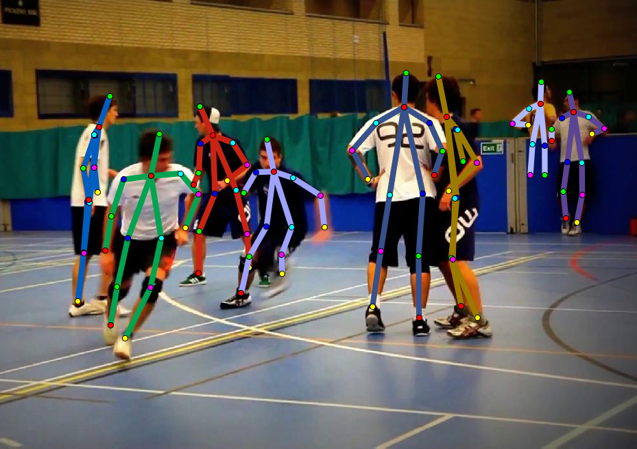
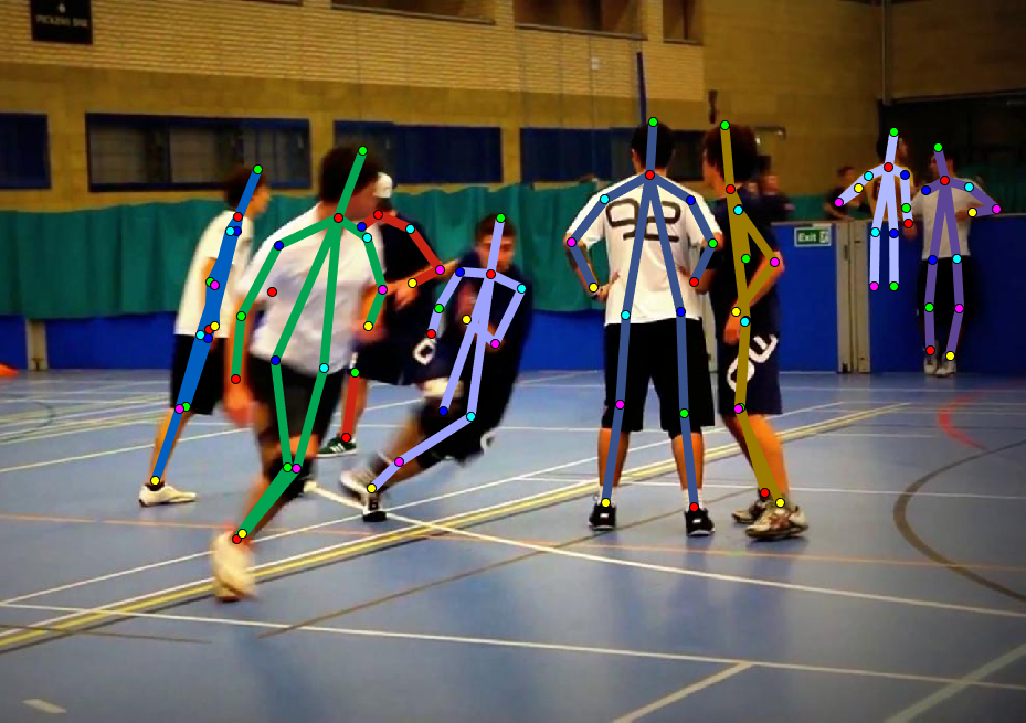
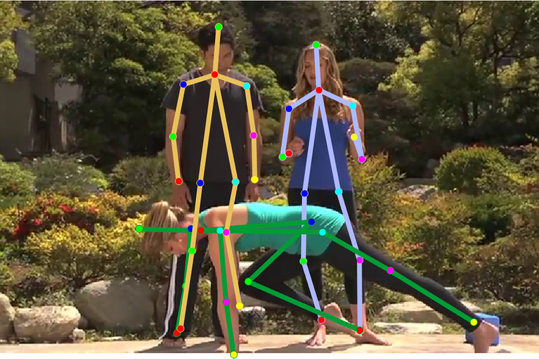
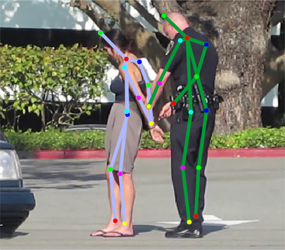
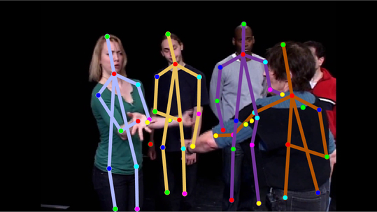
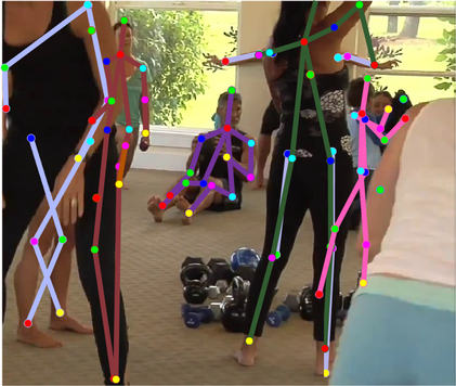
One of the key challenges in such scenes is that people might overlap and only a subset of joints of the person might be visible in each frame either due to person-person occlusion or truncation by image boundaries (c.f. Fig. 1). Arguably, resolving such cases correctly requires reasoning beyond purely geometric information on the arrangement of body joints in the image, and requires incorporation of a variety of image cues and joint modeling of several persons.

Figure 1: Example articulated tracking results of our approach.

The design of our model is motivated by two factors. We would like to leverage bottom-up end-to-end learning to directly capture image information. At the same time we aim to address a complex multi-person articulated tracking problem that does not naturally lend itself to an end-to-end prediction task and for which training data is not available in the amounts usually required for end-to-end learning.

To leverage the available image information we learn a model for associating a body joint to a specific person in an end-to-end fashion relying on a convolutional network. We then incorporate these part-to-person association responses into a framework for jointly reasoning about assignment of body joints within the image and over time. To that end we use the graph partitioning formulation that has been used for people tracking and pose estimation in the past [25, 23], but has not been shown to enable articulated people tracking.

To facilitate efficient inference in video we resort to fast inference methods based on local combinatorial optimization [20] and aim for a sparse model that keeps the number of connections between variables to a minimum. As we demonstrate, in combination with feed-forward reasoning for joint-to-person association this allows us to achieve substantial speed-ups compared to state-of-the-art [14] while maintaining the same level of accuracy.

The main contribution of this work is a new articulated tracking model that operates by bottom-up assembly of part detections within each frame and over time. In contrast to [12, 22] this model is suitable for scenes with an unknown number of subjects and reasons jointly across multiple people incorporating inter-person exclusion constraints and propagating strong observations to neighboring frames.

Our second contribution is a formulation for single-frame pose estimation that relies on a sparse graph between body parts and a mechanism for generating body-part proposals conditioned on a person’s location. This is in contrast to state-of-the-art approaches [23, 14] that perform expensive inference in a full graph and rely on generic bottom-up proposals. We demonstrate that a sparse model with a few spatial edges performs competitively with a fully-connected model while being much more efficient. Notably, a simple model that operates in top-down/bottom-up fashion exceeds the performance of a fully-connected model while being $24$x faster at inference time (cf. Tab. 3). This is due to offloading of a large share of the reasoning about body-part association onto a feed-forward convolutional architecture.

Finally, we contribute a new challenging dataset for evaluation of articulated body joint tracking in crowded realistic environments with multiple overlapping people.

Related work. Convolutional networks have emerged as an effective approach to localizing body joints of people in images [28, 29, 21, 14] and have also been extended for joint estimation of body configurations over time [12], and 3D pose estimation in outdoor environments in multi-camera setting [10, 11].

Current approaches are increasingly effective for estimating body configurations of single people [28, 29, 21, 5, 12] achieving high accuracies on this task, but are still failing on fast moving and articulated limbs. More complex recent models jointly reason about entire scenes [23, 14, 16], but are too complex and inefficient to directly generalize to image sequences. Recent feed-forward models are able to jointly infer body joints of the same person and even operate over time [12] but consider isolated persons only and do not generalize to the case of multiple overlapping people. Similarly, [6, 22] consider a simplified task of tracking upper body poses of isolated upright individuals.

We build on recent CNN detectors [14] that are effective in localizing body joints in cluttered scenes and explore different mechanisms for assembling the joints into multiple person configurations. To that end we rely on a graph partitioning approach closely related to [25, 23, 14]. In contrast to [25] who focus on pedestrian tracking, and [23, 14] who perform single frame multi-person pose estimation, we solve a more complex problem of articulated multi-person pose tracking.

Earlier approaches to articulated pose tracking in monocular videos rely on hand-crafted image representations and focus on simplified tasks, such as tracking upper body poses of frontal isolated people [24, 31, 27, 8], or tracking walking pedestrians with little degree of articulation [2, 3]. In contrast, we address a harder problem of multi-person articulated pose tracking and do not make assumptions about the type of body motions or activities of people. Our approach is closely related to [17] who propose a similar formulation based on graph partitioning. Our approach differs from [17] primarily in the type of body-part proposals and the structure of the spatio-temporal graph. In our approach we introduce a person-conditioned model that is trained to associate body parts of a specific person already at the detection stage. This is in contrast to the approach of [17] that relies on the generic body-part detectors [14].

Overview. Our model consists of the two components: (1) a convolutional network for generating body part proposals and (2) an approach to group the proposals into spatio-temporal clusters. In Sec. 2 we introduce a general formulation for multi-target tracking that follows [25] and allows us to define pose estimation and articulated tracking in a unified framework. We then describe the details of our articulated tracking approach in Sec. 3, and introduce two variants of our formulation: bottom-up (BU) and top-down/bottom-up (TD/BU). We present experimental results in Sec. 4.

2 Tracking by Spatio-temporal Grouping

Our body part detector generates a set of proposals $D=\{\mathbf{d}_{i}\}$ for each frame of the video. Each proposal is given by $\mathbf{d}_{i}=(t_{i},d^{pos}_{i},\pi_{i},\tau_{i})$, where $t_{i}$ denotes the index of the video frame, $d^{pos}_{i}$ is the spatial location of the proposal in image coordinates, $\pi_{i}$ is the probability of correct detection, and $\tau_{i}$ is the type of the body joint (e.g. ankle or shoulder).

Let $G=(D,E)$ be a graph whose nodes $D$ are the joint detections in a video and whose edges $E$ connect pairs of detections that hypothetically correspond to the same target.

The output of the tracking algorithm is a subgraph $G^{\prime}=(D^{\prime},E^{\prime})$ of $G$, where $D^{\prime}$ is a subset of nodes after filtering redundant and erroneous detections and $E^{\prime}$ are edges linking nodes corresponding to the same target. We specify $G^{\prime}$ via binary variables $x\in\{0,1\}^{D}$ and $y\in\{0,1\}^{E}$ that define subsets of edges and nodes included in $G^{\prime}$. In particular each track will correspond to a connected component in $G^{\prime}$.

As a general way to introduce constraints on edge configurations that correspond to a valid tracking solution we introduce a set $Z\subseteq\{0,1\}^{D\cup E}$ and define a combination of edge and node indicator variables to be feasible if and only if $(x,y)\in Z$. An example of a constraint encoded through $Z$ is that endpoint nodes of an edge included by $y$ must also be included by $x$. Note that the variables $x$ and $y$ are coupled though $Z$. Moreover, assuming that $(x,y)\in Z$ we are free to set components of $x$ and $y$ independently to maximize the tracking objective.

Given image observations we compute a set of features for each node and edge in the graph. We denote such node and edge features as $f$ and $g$ respectively. Assuming independence of the feature vectors the conditional probability of indicator functions $x$ of nodes and $y$ of edges given features $f$ and $g$ and given a feasible set $Z$ is given by

$$p(x,y|f,g,Z)\propto p(Z|x,y)\prod_{d\in D}p(x_{d}|f^{d})\prod_{e\in E}p(y_{e}|g^{e}),$$ (1)

where $p(Z|x,y)$ assigns a constant non-zero probability to every feasible solution and is equal to zero otherwise. Minimizing the negative log-likelihood of Eq. 1 is equivalent to solving the following integer-linear program:

$$\min_{\begin{array}[]{c}\scriptstyle(x,y)\in Z\end{array}}\sum_{d\in D}c_{d}x_{d}+\sum_{e\in E}d_{e}y_{e}\enspace,$$ (3)

where $c_{d}=\log\frac{p(x_{d}=1|f^{d})}{p(x_{d}=0|f^{d})}$ is the cost of retaining $d$ as part of the solution, and $d_{e}=\log\frac{p(y_{e}=1|g^{e})}{p(y_{e}=0|g^{e})}$ is the cost of assigning the detections linked by an edge $e$ to the same track.

We define the set of constraints $Z$ as in [25]:

$$\quad\forall e=vw\in E:\quad y_{vw}\leq x_{v}$$ (4)

$$\quad\forall e=vw\in E:\quad y_{vw}\leq x_{w}$$ (5)

$$\quad\forall C\in\mathrm{cycles}(G)\ \forall e\in C:\$$

$$\qquad\quad(1-y_{e})\leq\sum_{e^{\prime}\in C\setminus\{e\}}(1-y_{e^{\prime}})$$ (6)

Jointly with the objective in Eq. 3 the constraints (4)-(6) define an instance of the minimum cost subgraph multicut problem [25]. The constraints (4) and (5) ensure that assignment of node and edge variables is consistent. The constraint (6) ensures that for every two nodes either all or none of the paths between these nodes in graph $G$ are contained in one of the connected components of subgraph $G^{\prime}$. This constraint is necessary to unambigously assign person identity to a body part proposal based on its membership in a specific connnected component of $G^{\prime}$.

3 Articulated Multi-person Tracking

(a)	(b)	(c)

Figure 2: Visualization of (a) sparse connectivity, (b) attractive-repulsive edges and (c) temporal edges in our model. We show only a subset of attractive/repulsive and temporal edges for clarity.

Figure 3: (a) Processing stages of the Top-Down model shown for an example with significantly overlapping people. Left: Heatmaps for the chin (=root part) used to condition the CNN on the location of the person in the back (top) and in the front (bottom). Middle: Output heatmaps for all body parts, notice the ambiguity in estimates of the arms of the front person. Right: TD predictions for each person. (b) Example of the Top-Down/Bottom-Up graph. Red dotted line represents the must-cut constraint. Note that body part proposals of different type are connected to person nodes but not between each other. (c) Top-Down/Bottom-Up predictions. Notice that the TD/BU inference correctly assigns the forearm joints of the frontal person.

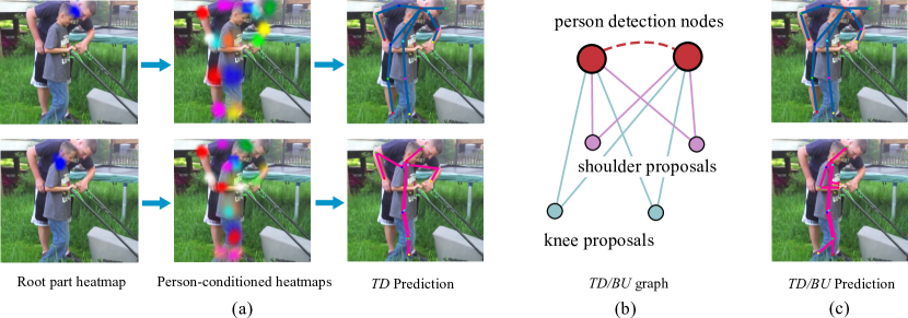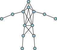
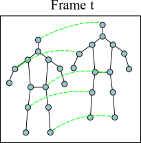
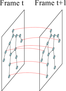
In Sec. 2 we introduced a general framework for multi-object tracking by solving an instance of the subgraph multicut problem. The subgraph multicut problem is NP-hard, but recent work [25, 20] has shown that efficient approximate inference is possible with local search methods. The framework allows for a variety of graphs and connectivity patterns. Simpler connectivity allows for faster and more efficient processing at the cost of ignoring some of the potentially informative dependencies between model variables. Our goal is to design a model that is efficient, with as few edges as possible, yet effective in crowded scenes, and that allows us to model temporal continuity and inter-person exclusion. Our articulated tracking approach proceeds by constructing a graph $G$ that couples body part proposals within the same frame and across neighboring frames. In general the graph $G$ will have three types of edges: (1) cross-type edges shown in Fig. 2 (a) and Fig. 3 (b) that connect two parts of different types, (2) same-type edges shown in Fig. 2 (b) that connect two nodes of the same type in the same image, and (3) temporal edges shown in Fig. 2 (c) that connect nodes in the neighboring frames.

We now define two variants of our model that we denote as Bottom-Up (BU) and Top-Down/Bottom-Up (TD/BU). In the BU model the body part proposals are generated with our publicly available convolutional part detector [14]. In the TD/BU model we substitute these generic part detectors with a new convolutional body-part detector that is trained to output consistent body configurations conditioned on the person location. This alows to further reduce the complexity of the model graph since the task of associating body parts is addressed within the proposal mechanism. As we show in Sec. 4 this leads to considerable gains in performance and allows for faster inference. Note that the BU and TD/BU models have identical same-type and temporal pairwise terms, but differ in the form of cross-type pairwise terms, and the connectivity of the nodes in $G$. For both models we rely on the solver from [20] for inference.

3.1 Bottom-Up Model (BU).

For each body part proposal $\mathbf{d}_{i}$ the detector outputs image location, probability of detection $\pi_{i}$, and a label $\tau_{i}$ that indicates the type of the detected part (e.g. shoulder or ankle). We directly use the probability of detection to derive the unary costs in Eq. 3 as $c_{d_{i}}=\log(\pi_{i}/(1-\pi_{i}))$. Image features $f^{d}$ in this case correspond to the image representation generated by the convolutional network.

We consider two connectivity patterns for nodes in the graph $G$. We either define edges for every pair of proposals which results in a fully connected graph in each image. Alternatively we obtain a sparse version of the model by defining edges for a subset of part types only as is shown in Fig. 2 (a). The rationale behind the sparse version is to obtain a simpler and faster version of the model by omitting edges between parts that carry little information about each other’s image location (e.g. left ankle and right arm).

Edge costs. In our Bottom-Up model the cost of the edges $d_{e}$ connecting two body part detections $\mathbf{d}_{i}$ and $\mathbf{d}_{j}$ is defined as a function of the detection types $\tau_{i}$ and $\tau_{j}$. Following [14] we thus train for each pair of part types a regression function that predicts relative image location of the parts in the pair. The cost $d_{e}$ is given by the output of the logistic regression given the features computed from offset and angle of the predicted and actual location of the other joint in the pair. We refer to [14] for more details on these pairwise terms.

Note that our model generalizes [25] in that the edge cost depends on the type of nodes linked by the edge. It also generalizes [23, 14] by allowing $G$ to be sparse. This is achieved by reformulating the model with a more general type of cycle constraint (6), in contrast to simple triangle inequalities used in [23, 14].

3.2 Top-Down/Bottom-up Model (TD/BU)

Figure 4: CNN architecture based on ResNet-101 for computing person conditioned proposals and pairwise terms. SP block for shoulders at conv_4_8 is omitted for clarity.

We now introduce a version of our model that operates by first generating body part proposals conditioned on the locations of people in the image and then performing joint reasoning to group these proposals into spatio-temporal clusters corresponding to different people. We follow the intuition that it is considerably easier to identify and detect individual people (e.g. by detecting their heads) compared to correctly associating body parts such as ankles and wrists to each person. We select person’s head as a root part that is responsible for representing the person location, and delegate the task of identifying body parts of the person corresponding to a head location to a convolutional network.

The structure of TD/BU model is illustrated in Fig. 3 (b) for the simplified case of two distinct head detections. Let us denote the set of all root part detections as $D^{root}=\{d_{i}^{root}\}$. For each pair of the root nodes we explicitly set the corresponding edge indicator variables $y_{d_{j}^{root},d_{k}^{root}}=0$. This implements a “must-not-link” constraint between these nodes, and in combination with the cycle inequality (6) implies that each proposal can be connected to one of the “person nodes” only. The cost for an edge connecting detection proposal $\mathbf{d}_{k}$ and a “person node” $d_{i}^{root}$ is based on the conditional distribution $p_{d_{k}^{c}}(d_{k}^{pos}|d_{i}^{root})$ generated by the convolutional network. The output of such network is a set of conditional distributions, one for each node type. We augment the graph $G$ with attractive/repulsive and temporal terms as described in Sec. 3.3 and Sec. 3.4 and set the unary costs for all indicator variables $x_{d}$ to a constant. Any proposal not connected to any of the root nodes is excluded from the final solution. We use the solver from [20] for consistency, but a simpler KL-based solver as in [25, 19] could be used as well since the TD/BU model effectively ignores the unary variables $x_{d}$. The processing stages of TD/BU model are shown in Fig. 3. Note that the body-part heatmaps change depending on the person-identity signal provided by the person’s neck, and that the bottom-up step was able to correct the predictions on the forearms of the front person.

Implementation details. For head detection, we use a version of our model that contains the two head parts (neck and head top). This makes our TD/BU model related to the hierarchical model defined in [14] that also uses easier-to-detect parts to guide the rest of the inference process. However here we replace all the stages in the hierarchical inference except the first one with a convolutional network.

The structure of the convolutional network used to generate person-conditioned proposals is shown on Fig. 4. The network uses the ResNet-101 from [13] that we modify to bring the stride of the network down to 8 pixels [14]. The network generates predictions for all body parts after the conv4_4 block. We use the cross-entropy binary classification loss at this stage to predict the part heatmaps. At each training iteration we forward pass an image with multiple people potentially in close proximity to each other. We select a single person from the image and condition the network on the person’s neck location by zeroing out the heatmap of the neck joint outside the ground-truth region. We then pass the neck heatmap through a convolutional layer to match the dimensionality of the feature channels and add them to the main stream of the ResNet. We finally add a joint prediction layer at the end of the network with a loss that considers predictions to be correct only if they correspond to the body joints of the selected person.

Spatial propagation (SP). In our network the person identity signal is provided by the location of the head. In principle the receptive field size of the network is large enough to propagate this signal to all body parts. However we found that it is useful to introduce an additional mechanism to propagate the person identity signal. To that end we inject intermediate supervision layers for individual body parts arranged in the order of kinematic proximity to the root joint (Fig. 4). We place prediction layers for shoulders at conv4_8, for elbows and hips at conv4_14 and for knees at conv4_18. We empirically found that such an explicit form of spatial propagation significantly improves performance on joints such as ankles, that are typically far from the head in the image space (see Tab. 2 for details).

Training. We use Caffe’s [18] ResNet implementation and initialize from the ImageNet-pre-trained models. Networks are trained on the MPII Human Pose dataset [1] with SGD for 1M iterations with stepwise learning rate (lr=0.002 for 400k, lr=0.0002 for 300k and lr=0.0001 for 300k).

3.3 Attractive/Repulsive Edges

Attractive/repulsive edges are defined between two proposals of the same type within the same image. The costs of these edges is inversely-proportional to distance [14]. The decision to group two nodes is made based on the evidence from the entire image, which is in contrast to typical non-maximum suppression based on the state of just two detections. Inversely, these edges prevent grouping of multiple distant hypothesis of the same type, e.g. prevent merging two heads of different people.

3.4 Temporal Model

Regardless of the type of within frame model (BU or TD/BU) we rely on the same type of temporal edges that connect nodes of the same type in adjacent frames. We derive the costs for such temporal edges via logistic regression. Given the feature vector $g_{ij}$ the probability that the two proposals $\mathbf{d}_{i}$ and $\mathbf{d}_{j}$ in adjacent frames correspond to the same body part is given by: $p(y_{ij}=1|g_{ij})=1/(1+\exp(-\langle\omega_{t},g_{ij}\rangle))$, where $g_{ij}=(\Delta_{ij}^{L2},\Delta_{ij}^{Sift},\Delta_{ij}^{DM},\tilde{\Delta}_{ij}^{DM})$, and $\Delta_{ij}^{L2}=\|d^{pos}_{i}$ - $d^{pos}_{j}\|_{2}$, $\Delta_{ij}^{Sift}$ is Euclidean distance between the SIFT descriptors computed at $d^{pos}_{i}$ and $d^{pos}_{j}$, and $\Delta_{ij}^{DM}$ and $\tilde{\Delta}_{ij}^{DM}$ measure the agreement with the dense motion field computed with the DeepMatching approach of [30].

For SIFT features we specify the location of the detection proposal, but rely on SIFT to identify the local orientation. In cases with multiple local maxima in orientation estimation we compute SIFT descriptor for each orientation and set $\Delta_{ij}^{Sift}$ to the minimal distance among all pairs of descriptors. We found that this makes the SIFT distance more robust in the presence of rotations of the body limbs.

We define the features $\Delta_{ij}^{DM}$ and $\tilde{\Delta}_{ij}^{DM}$ as in [26]. Let $R_{i}=R(\mathbf{d}_{i})$ be an squared image region centered on the part proposal $\mathbf{d}_{i}$. We define $\Delta_{ij}^{DM}$ as a ratio of the number of point correspondences between the regions $R_{i}$ and $R_{j}$ and the total number of point correspondences in either of them. Specifically, let $C=\{c^{k}|k=1,\ldots,K\}$ be a set of point correspondences between the two images computed with DeepMatching, where $c^{k}=(c^{k}_{1},c^{k}_{2})$ and $c^{k}_{1}$ and $c^{k}_{2}$ denote the corresponding points in the first and second image respectively. Using this notation we define:

$$\Delta_{ij}^{DM}=\frac{|\{c_{k}|c^{k}_{1}\in R_{i}\land c^{k}_{2}\in R_{j}\}|}{|\{c_{k}|c^{k}_{1}\in R_{i}\}|+|\{c_{k}|c^{k}_{2}\in R_{j}\}|}.$$ (7)

The rationale behind computing $\Delta_{ij}^{DM}$ by aggregating across multiple correspondences is to make the feature robust to outliers and to inaccuracies in body part detection. $\tilde{\Delta}_{ij}^{DM}$ is defined analogously, but using the DeepMatching correspondences obtained by inverting the order of images.

Discussion. As we demonstrate in Sec. 4, we found the set of features described above to be complementary to each other. Euclidean distance between proposals is informative for finding correspondences for slow motions, but fails for faster motions and in the presence of multiple people. DeepMatching is usually effective in finding corresponding regions between the two images, but occasionally fails in the case of sudden background changes due to fast motion or large changes in body limb orientation. In these cases SIFT is often still able to provide a meaningful measure of similarity due to its rotation invariance.

4 Experiments

4.1 Datasets and evaluation measure

Single frame. We evaluate our single frame models on the MPII Multi-Person dataset [1]. We report all intermediate results on a validation set of $200$ images sampled uniformly at random (MPII Multi-Person Val), while major results and comparison to the state of the art are reported on the test set.

Video. In order to evaluate video-based models we introduce a novel “MPII Video Pose” dataset. To this end we manually selected challenging keyframes from MPII Multi-Person dataset. Selected keyframes represent crowded scenes with highly articulated people engaging in various dynamic activities. In addition to each keyframe, we include +/-$10$ neighboring frames from the corresponding publicly available video sequences, and annotate every second frame. Each body pose was annotated following the standard annotation procedure [1], while maintaining person identity throughout the sequence. In contrast to MPII Multi-Person where some frames may contain non-annotated people, we annotate all people participating in the activity captured in the video, and add ignore regions for areas that contain dense crowds (e.g. static spectators in the dancing sequences). In total, our dataset consists of $28$ sequences with over $2,000$ annotated poses.

Evaluation details. The average precision (AP) measure [23] is used for evaluation of pose estimation accuracy. For each algorithm we also report run time $\tau_{\mbox{\tiny{CNN}}}$ of the proposal generation and $\tau_{\mbox{\scriptsize{graph}}}$ of the graph partitioning stages. All time measurements were conducted on a single core Intel Xeon $2.70$GHz. Finally we also evaluate tracking perfomance using standard MOTA metric [4].

Evaluation on our “MPII Video Pose” dataset is performed on the full frames using the publicly available evaluation kit of [1]. On MPII Multi-Person we follow the official evaluation protocol and evaluate on groups using the provided rough group location and scale.

4.2 Single-frame models

Setting	Head	Sho	Elb	Wri	Hip	Knee	Ank	AP	$\tau_{\mbox{\tiny{CNN}}}$	$\tau_{\mbox{\scriptsize{graph}}}$
BU-full, label	90.0	84.9	71.1	58.4	69.7	64.7	54.7	70.5	0.18	3.06
BU-full	91.2	86.0	72.9	61.5	70.4	65.4	55.5	71.9	0.18	0.38
BU-sparse	91.1	86.5	70.7	58.1	69.7	64.7	53.8	70.6	0.18	0.22
TD/BU + SP	92.2	86.1	72.8	63.0	74.0	66.2	58.4	73.3	0.94	0.08

Table 1: Effects of various variants of BU model on pose estimation performance (AP) on MPII Multi-Person Val and comparison to the best variant of TD/BUmodel.

We compare the performance of different variants of our Bottom-Up (BU) and Top-Down/Bottom-Up (TD/BU) models introduced in Sec. 3.1 and Sec. 3.2. For BU we consider a model that (1) uses a fully-connected graph with up to $1,000$ detection proposals and jointly performs partitioning and body-part labeling similar to [14] (BU-full, label); (2) is same as (1), but labeling of detection proposals is done based on detection score (BU-full); (3) is same as (2), but uses a sparsely-connected graph (BU-sparse). The results are shown in Tab. 1. BU-full, label achieves $70.5$% AP with a median inference run-time $\tau_{\mbox{\scriptsize{graph}}}$ of $3.06$ s/f. BU-full achieves $8\times$ run-time reduction ($0.38$ vs. $3.06$ s/f): pre-labeling detection candidates based on detection score significantly reduces the number of variables in the problem graph. Interestingly, pre-labeling also improves the performance ($71.9$ vs. $70.5$% AP): some of the low-scoring detections may complicate the search for an optimal labeling. BU-sparse further reduces run-time ($0.22$ vs. $0.38$ s/f), as it reduces the complexity of the initial problem by sparsifying the graph, at a price of a drop in performance ($70.6$ vs. $71.9$% AP).

In Tab. 2 we compare the variants of the TD/BU model. Our TD approach achieves $71.7$% AP, performing on par with a more complex BU-full. Explicit spatial propagation (TD+SP) further improves the results ($72.5$ vs. $71.7$% AP). The largest improvement is observed for ankles: progressive prediction that conditions on the close-by parts in the tree hierarchy reduces the distance between the conditioning signal and the location of the predicted body part and simplifies the prediction task. Performing inference (TD/BU+SP) improves the performance to $73.3$% AP, due to more optimal assignment of part detection candidates to corresponding persons. Graph simplification in TD/BU allows to further reduce the inference time for graph partitioning ($0.08$ vs. $0.22$ for BU-sparse).

Setting	Head	Sho	Elb	Wri	Hip	Knee	Ank	AP
TD	91.6	84.7	72.9	63.2	72.3	64.7	52.8	71.7
TD + SP	90.7	85.0	72.0	63.1	73.1	65.0	58.3	72.5
TD/BU + SP	92.2	86.1	72.8	63.0	74.0	66.2	58.4	73.3

Table 2: Effects of various versions of TD/BU model on pose estimation performance (AP) on MPII Multi-Person Val.

Setting	Head	Sho	Elb	Wri	Hip	Knee	Ank	AP	$\tau_{\mbox{\scriptsize{graph}}}$
BU-full	91.5	87.8	74.6	62.5	72.2	65.3	56.7	72.9	0.12
TD/BU+ SP	88.8	87.0	75.9	64.9	74.2	68.8	60.5	74.3	0.005
DeeperCut [14]	79.1	72.2	59.7	50.0	56.0	51.0	44.6	59.4	485
DeeperCut [15]	89.4	84.5	70.4	59.3	68.9	62.7	54.6	70.0	485
Iqbal&Gall [16]	58.4	53.9	44.5	35.0	42.2	36.7	31.1	43.1	10

Table 3: Pose estimation results (AP) on MPII Multi-Person Test.

Single Frame
Tracking
	(a)	(b)	(c)	(d)
Single Frame
Tracking
	(e)	(f)	(g)	(h)

Figure 5: Qualitative comparison of results using single frame based model (BU-sparse) vs. articulated tracking (BU-sparse+temporal). See http://youtube.com/watch?v=eYtn13fzGGo for the supplemental material showcasing our results.

Comparison to the State of the Art. We compare the proposed single-frame approaches to the state of the art on MPII Multi-Person Test and WAF [9] datasets. Comparison on MPII is shown in Tab. 3. Both BU-full and TD/BU improve over the best published result of DeeperCut [15], achieving $72.9$ and $74.3$% AP respectively vs. $70.0$% AP by DeeperCut. For the TD/BU the improvements on articulated parts (elbows, wrists, ankles, knees) are particularly pronounced. We argue that this is due to using the network that is directly trained to disambiguate body parts of different people, instead of using explicit geometric pairwise terms that only serve as a proxy to person’s identity. Overall, the performance of our best TD/BU method is noticeably higher ($74.3$ vs. $70.0$% AP). Remarkably, its run-time $\tau_{\mbox{\scriptsize{graph}}}$ of graph partitioning stage is $5$ orders of magnitude faster compared to DeeperCut. This speed-up is due to two factors. First, TD/BU relies on a faster solver [20] that tackles the graph-partitioning problem via local search, in contrast to the exact solver used in [14]. Second, in the case of TD/BU model the graph is sparse and a large portion of the computation is performed by the feed-forward CNN introduced in Sec. 3.2. On WAF [9] dataset TD/BU substantially improves over the best published result ($87.7$ vs. $82.0$% AP by [15]). We refer to supplemental material for details.

4.3 Multi-frame models

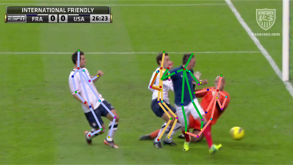
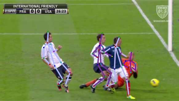
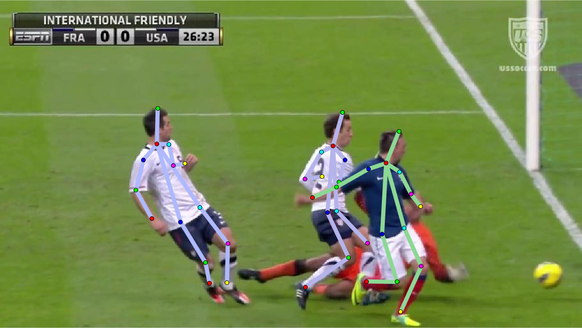
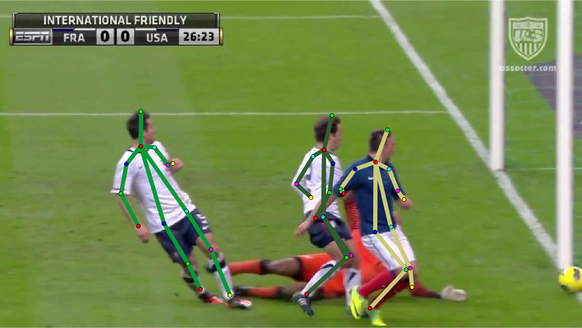
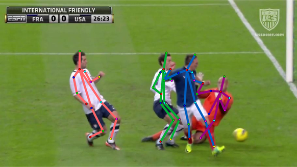
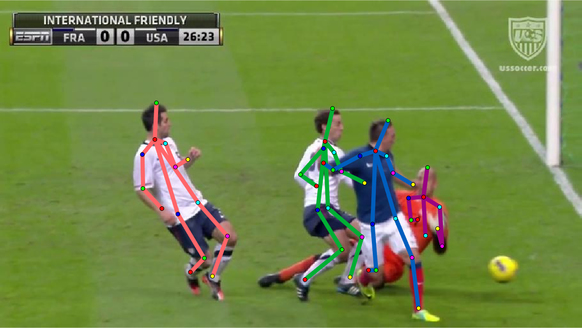
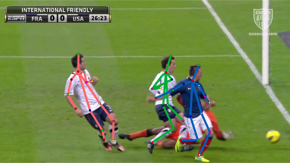
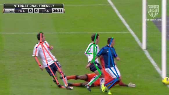
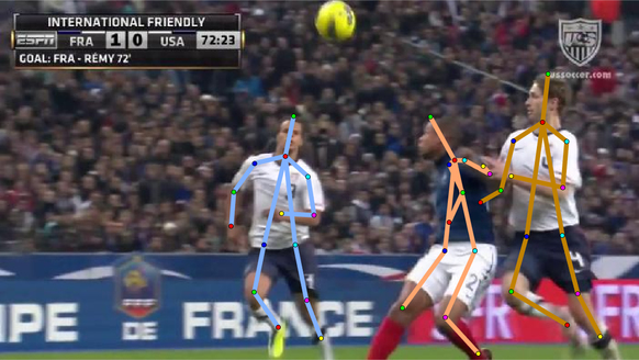
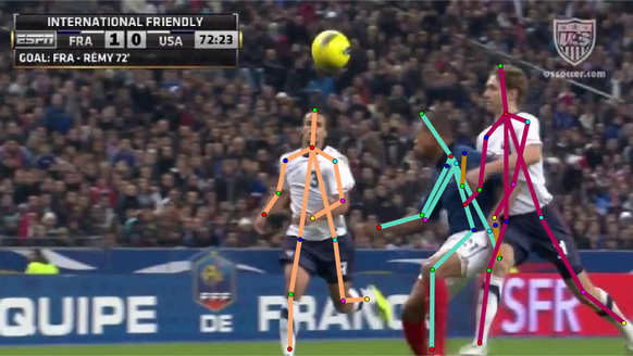
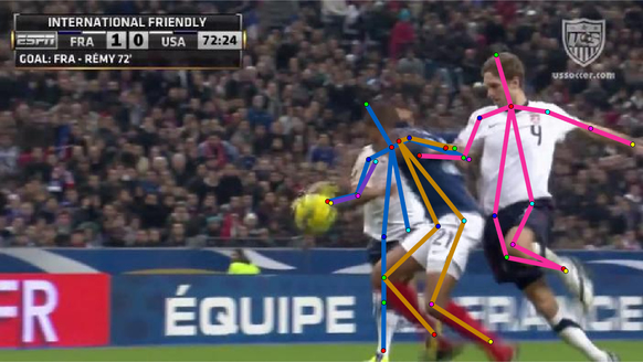
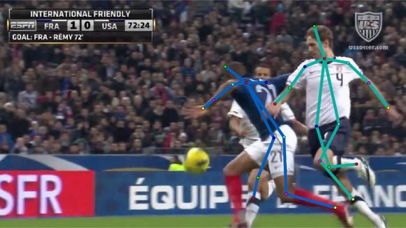
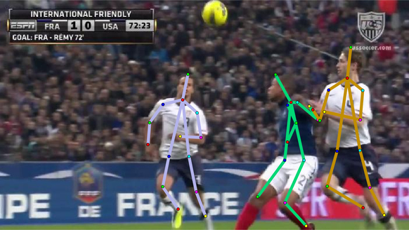
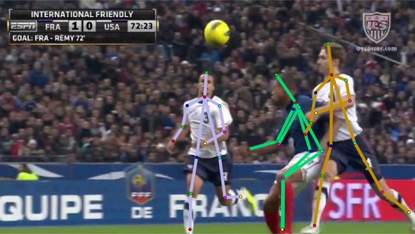
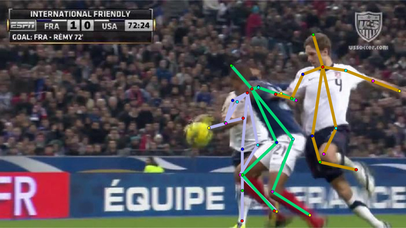
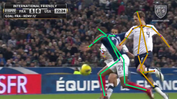
Comparison of video-based models. Performance of the proposed video-based models is compared in Tab. 4. Video-based models outperform single-frame models in each case. BU-full+temporal slightly outperforms BU-full, where improvements are noticeable for ankle, knee and head. BU-sparse+temporal noticeably improves over BU-sparse ($73.1$ vs. $71.6$% AP). We observe significant improvements on the most difficult parts such as ankles ($+3.9$% AP) and wrists ($+2.6$% AP). Interestingly, BU-sparse+temporal outperforms $\textit{BU-full}+\textit{temporal}$: longer-range connections such as, e.g., head to ankle, may introduce additional confusion when information is propagated over time. Finally, TD/BU+temporal improves over TD/BU ($+0.7$% AP). Similarly to BU-sparse+temporal, improvement is most prominent on ankles ($+1.8$% AP) and wrists ($+0.9$% AP). Note that even the single-frame TD/BU outperforms the best temporal BU model. We show examples of articulated tracking on “MPII Video Pose” in Fig. 5. Temporal reasoning helps in cases when image information is ambiguous due to close proximity of multiple people. For example the video-based approach succeeds in correctly localizing legs of the person in Fig. 5 (d) and (h).

Temporal features. We perform an ablative experiment on the “MPII Video Pose”  dataset to evaluate the individual contribution of the temporal features introduced in Sec. 3.4. The Euclidean distance alone achieves $72.1$ AP, adding DeepMatching features improves the resuls to $72.5$ AP, whereas the combination of all features achieves the best result of $73.1$ AP (details in supplemental material).

Setting	Head	Sho	Elb	Wri	Hip	Knee	Ank	AP
BU-full	84.0	83.8	73.0	61.3	74.3	67.5	58.8	71.8
+ temporal	84.9	83.7	72.6	61.6	74.3	68.3	59.8	72.2
BU-sparse	84.5	84.0	71.8	59.5	74.4	68.1	59.2	71.6
+ temporal	85.6	84.5	73.4	62.1	73.9	68.9	63.1	73.1
TD/BU+ SP	82.2	85.0	75.7	64.6	74.0	69.8	62.9	73.5
+ temporal	82.6	85.1	76.3	65.5	74.1	70.7	64.7	74.2

Table 4: Pose estimation results (AP) on “MPII Video Pose”.

Tracking evaluation. In Tab. 5 we present results of the evaluation of multi-person articulated body tracking. We treat each body joint of each person as a tracking target and measure tracking performance using a standard multiple object tracking accuracy (MOTA) metric [4] that incorporates identity switches, false positives and false negatives. We experimentally compare to a baseline model that first tracks people across frames and then performs per-frame pose estimation. To track a person we use a reduced version of our algorithm that operates on the two head joints only. This allows to achieve near perfect person tracking results in most cases. Our tracker still fails when the person head is occluded for multiple frames as it does not incorporate long-range connectivity between target hypothesis. We leave handling of long-term occlusions for the future work. For full-body tracking we use the same inital head tracks and add them to the set of body part proposals, while also adding must-link and must-cut constraints for the temporal edges corresponding to the head parts detections. The rest of the graph remains unchanged so that at inference time the body parts can be freely assigned to different person tracks. For the BU-sparse the full body tracking improves performance by $+5.9$ and $+5.8$ MOTA on wrists and ankles, and by $+5.0$ and $+2.4$ MOTA on elbows and knees respectively. TD/BU benefits from adding temporal connections between body parts as well, but to a lesser extent than BU-sparse. The most significant improvement is for ankles ($+1.4$ MOTA). BU-sparse also achieves the best overall score of $58.5$ compared to $55.9$ by TD/BU. This is surprising since TD/BU outperformed BU-sparse on the pose estimation task (see Tab. 1 and 3). We hypothesize that limited improvement of TD/BU could be due to balancing issues between the temporal and spatial pairwise terms that are estimated independently of each other.

Setting	Head	Sho	Elb	Wri	Hip	Knee	Ank	Average
Head track + BU-sparse	70.5	71.7	53.0	41.7	57.0	52.4	41.9	55.5
+ temporal	70.6	72.7	58.0	47.6	57.6	54.8	47.7	58.5
Head track + TD/BU	64.8	69.4	55.4	43.4	56.4	52.2	44.8	55.2
+ temporal	65.0	69.9	56.3	44.2	56.7	53.2	46.1	55.9

Table 5: Tracking results (MOTA) on the “MPII Video Pose”.

5 Conclusion

In this paper we introduced an efficient and effective approach to articulated body tracking in monocular video. Our approach defines a model that jointly groups body part proposals within each video frame and across time. Grouping is formulated as a graph partitioning problem that lends itself to efficient inference with recent local search techniques. Our approach improves over state-of-the-art while being substantially faster compared to other related work.

Acknowledgements. This work has been supported by the Max Planck Center for Visual Computing and Communication. The authors thank Varvara Obolonchykova and Bahar Tarakameh for their help in creating the video dataset.

Appendix A Additional Results on the MPII Multi-Person Dataset

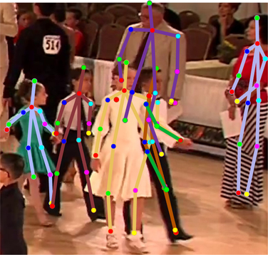
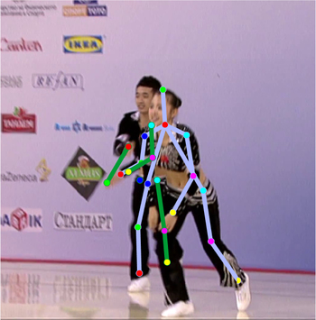
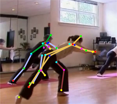
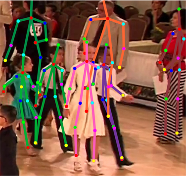
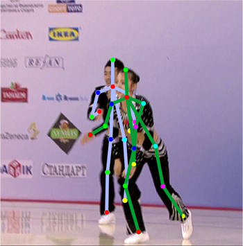
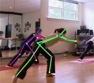
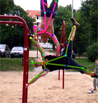
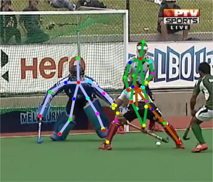
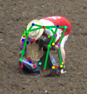
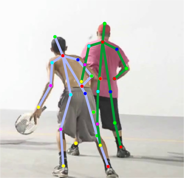
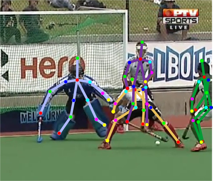
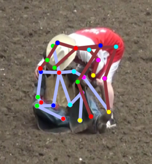
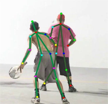
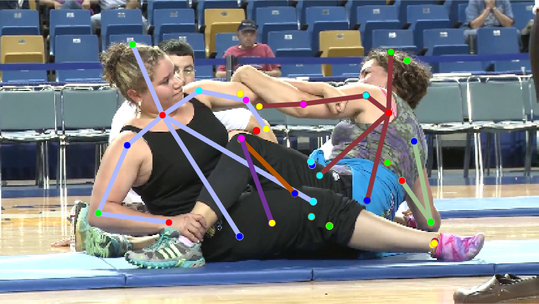
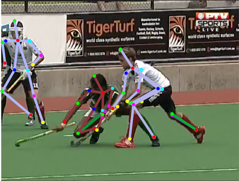
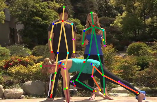
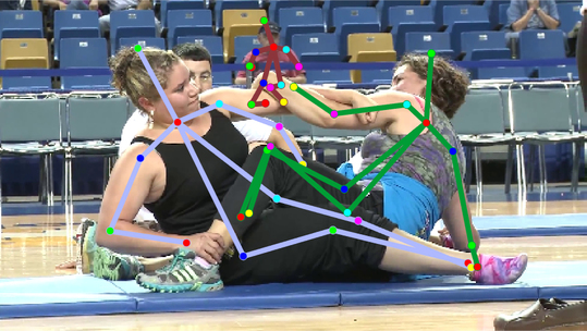
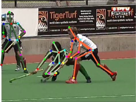
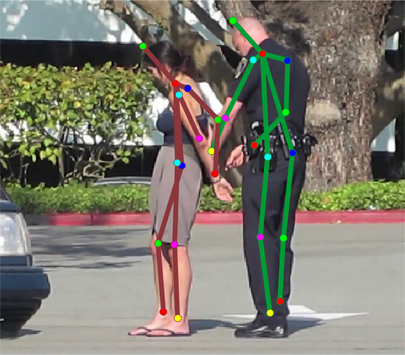
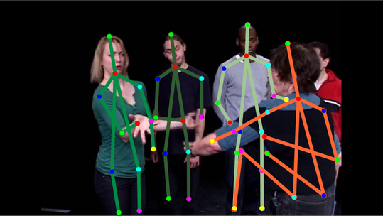
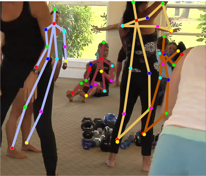
We perform qualitative comparison of the proposed single-frame based  TD/BU and BU-full methods on challenging scenes containing highly articulated and strongly overlapping individuals. Results are shown in Fig. 6 and Figure 7. The BU-full works well when persons are sufficiently separated (images 11 and 12). However, it fails on images where people significantly overlap (images 1-3, 5-10) or exhibit high degree of articulation (image 4). This is due to the fact that geometric image-conditioned pairwise may get confused in the presence of multiple overlapping individuals and thus mislead post-CNN bottom-up assembling of body poses. In contrast, TD/BU performs explicit modeling of person identity via top-dop bottom-up reasoning while offloading the larger share of the reasoning about body-part association onto feed-forward convolutional architecture, and thus is able to resolve such challenging cases. Interestingly, TD/BU is able to correctly predict lower limbs of people in the back through partial occlusion (image 3, 5, 7, 10). TD/BU model occasionally incorrectly assembles body parts in kinematically implausible manner (image 12), as it does not explicitly model geometric body part relations. Finally, both models fail in presense of high variations in scale (image 13). We envision that reasoning over multiple scales is likely to improve the results.

BU
TD/BU
	1	2	3	4

BU
TD/BU
	5	6	7

Figure 6: Qualitative comparison of single-frame based TD/BU and BU-full on MPII Multi-Person dataset.

BU
TD/BU
	8	9	10

BU
TD/BU
	11	12	13

Figure 7: Successfull (8-11) and failure (12-13) pose estimation results by single-frame based TD/BU and comparison to BU-full on MPII Multi-Person dataset.

Appendix B Results on the We Are Family dataset

Method	Head	Sho	Elb	Wri	Total
TD/BU	97.5	86.2	82.1	85.2	87.7
DeeperCut [14]	92.6	81.1	75.7	78.8	82.0
DeepCut [23]	76.6	80.8	73.7	73.6	76.2
Chen&Yuille [7]	83.3	56.1	46.3	35.5	55.3

Table 6: Pose estimation results (AP) on WAF dataset.

Setting	Head	Sho	Elb	Wri	Hip	Knee	Ank	AP
BU-sparse	84.5	84.0	71.8	59.5	74.4	68.1	59.2	71.6
+ det-distance	84.8	84.3	72.9	61.8	74.1	67.4	59.1	72.1
+ deepmatch	85.5	83.9	73.0	62.0	74.0	68.0	59.5	72.3
+ det-distance	85.1	83.6	72.2	61.5	74.4	68.8	62.2	72.5
+ sift-distance	85.6	84.5	73.4	62.1	73.9	68.9	63.1	73.1

Table 7: Effects of different temporal features on pose estimation performance (AP) (BU-sparse+temporal model) on our “MPII Video Pose”.

We compare our proposed TD/BU model to the state-of-the-art methods on the “We Are Family” (WAF) [9] dataset and present results in Table 6. We use evaluation protocol from [14] and report the AP evaluation measure. TD/BU model outperforms the best published results [14] across all body parts ($87.7$ vs $82.0$% AP) as well improves on articulated parts such as wrists ($+6.4$% AP) and elbows ($+6.4$% AP). We attribute that to the ability of top-down model to better learn part associations compared to explicit modeling geometric pairwise relations as in [14].

Appendix C Evaluation of temporal features.

We evaluate the importance of combining temporal features introduced in Sec. 3.4 of the paper on our Multi-Person Video dataset. To that end, we consider BU-sparse+temporal model and compare results to BU-sparse in Tab. 7. Single-frame BU-sparse achieves $71.6$% AP. It can be seen that using geometry based det-distance features slightly improves the results to $72.1$% AP, as it enables the propagation of information from neighboring frames. Using deepmatch features slightly improves the performance further as it helps to link the same body part of the same person over time based on the body part appearance. It is especially helpful in the case of fast motion where det-distance may fail. The combination of both geometry and appearance based features further improves the performance to $72.5$%, which shows their complementarity. Finally, adding the sift-distance feature improves the results to $73.1$%, since it copes better with the sudden changes in background and body part orientations. Overall, using a combination of temporal features in BU-sparse+temporal results in a $1.5$% AP improvement over the single-frame BU-sparse. This demonstrates the advantages of the proposed approach to improve pose estimation performance using temporal information.

References

- [1] M. Andriluka, L. Pishchulin, P. Gehler, and B. Schiele. 2d human pose estimation: New benchmark and state of the art analysis. In CVPR’14.
- [2] M. Andriluka, S. Roth, and B. Schiele. People-tracking-by-detection and people-detection-by-tracking. In CVPR’08.
- [3] M. Andriluka, S. Roth, and B. Schiele. Monocular 3d pose estimation and tracking by detection. In CVPR, 2010.
- [4] K. Bernardin and R. Stiefelhagen. Evaluating multiple object tracking performance: The CLEAR MOT metrics. Image and Video Processing, 2008(1):1–10, May 2008.
- [5] A. Bulat and G. Tzimiropoulos. Human pose estimation via convolutional part heatmap regression. In ECCV’16.
- [6] J. Charles, T. Pfister, D. Magee, and A. Hogg, D. Zisserman. Personalizing human video pose estimation. In CVPR’16.
- [7] X. Chen and A. Yuille. Parsing occluded people by flexible compositions. In CVPR, 2015.
- [8] A. Cherian, J. Mairal, K. Alahari, and C. Schmid. Mixing body-part sequences for human pose estimation. In CVPR’14.
- [9] M. Eichner and V. Ferrari. We are family: Joint pose estimation of multiple persons. In ECCV’10.
- [10] A. Elhayek, E. Aguiar, A. Jain, J. Tompson, L. Pishchulin, M. Andriluka, C. Bregler, B. Schiele, and C. Theobalt. Efficient convnet-based marker-less motion capture in general scenes with a low number of cameras. In CVPR’15.
- [11] A. Elhayek, E. Aguiar, A. Jain, J. Tompson, L. Pishchulin, M. Andriluka, C. Bregler, B. Schiele, and C. Theobalt. Marconi - convnet-based marker-less motion capture in outdoor and indoor scenes.
- [12] G. Gkioxari, A. Toshev, and N. Jaitly. Chained predictions using convolutional neural networks.
- [13] K. He, X. Zhang, S. Ren, and J. Sun. Deep residual learning for image recognition. arXiv preprint arXiv:1512.03385, 2015.
- [14] E. Insafutdinov, L. Pishchulin, B. Andres, M. Andriluka, and B. Schiele. Deepercut: A deeper, stronger, and faster multi-person pose estimation model. In ECCV’16.
- [15] E. Insafutdinov, L. Pishchulin, B. Andres, M. Andriluka, and B. Schiele. Deepercut: A deeper, stronger, and faster multi-person pose estimation model. arXiv’16.
- [16] U. Iqbal and J. Gall. Multi-person pose estimation with local joint-to-person associations. In ECCVw’16.
- [17] U. Iqbal, A. Milan, and J. Gall. Posetrack: Joint multi-person pose estimation and tracking. In CVPR’17.
- [18] Y. Jia, E. Shelhamer, J. Donahue, S. Karayev, J. Long, R. Girshick, S. Guadarrama, and T. Darrell. Caffe: Convolutional architecture for fast feature embedding. arXiv preprint arXiv:1408.5093, 2014.
- [19] M. Keuper, E. Levinkov, N. Bonneel, G. Lavoué, T. Brox, and B. Andres. Efficient decomposition of image and mesh graphs by lifted multicuts. In ICCV’15.
- [20] E. Levinkov, J. Uhrig, S. Tang, M. Omran, E. Insafutdinov, A. Kirillov, C. Rother, T. Brox, B. Schiele, and B. Andres. Joint graph decomposition & node labeling: Problem, algorithms, applications. In CVPR’17.
- [21] A. Newell, K. Yang, and J. Deng. Stacked hourglass networks for human pose estimation. In ECCV’16.
- [22] T. Pfister, J. Charles, and A. Zisserman. Flowing convnets for human pose estimation in videos. In ICCV’15.
- [23] L. Pishchulin, E. Insafutdinov, S. Tang, B. Andres, M. Andriluka, P. Gehler, and B. Schiele. Deepcut: Joint subset partition and labeling for multi person pose estimation. In CVPR’16.
- [24] B. Sapp, D. Weiss, and B. Taskar. Parsing human motion with stretchable models. In CVPR’11.
- [25] S. Tang, B. Andres, M. Andriluka, and B. Schiele. Subgraph decomposition for multi-target tracking. In CVPR, 2015.
- [26] S. Tang, B. Andres, M. Andriluka, and B. Schiele. Multi-person tracking by multicuts and deep matching. In BMTT, 2016.
- [27] R. Tokola, W. Choi, and S. Savarese. Breaking the chain: liberation from the temporal markov assumption for tracking human poses. In ICCV’13.
- [28] J. J. Tompson, A. Jain, Y. LeCun, and C. Bregler. Joint training of a convolutional network and a graphical model for human pose estimation. In NIPS’14.
- [29] S.-E. Wei, V. Ramakrishna, T. Kanade, and Y. Sheikh. Convolutional pose machines. In CVPR’16.
- [30] P. Weinzaepfel, J. Revaud, Z. Harchaoui, and C. Schmid. Deepflow: Large displacement optical flow with deep matching. In ICCV’13.
- [31] D. J. Weiss and B. Taskar. Learning adaptive value of information for structured prediction. In NIPS’13.