General models for rational cameras and the case of two-slit projections

Abstract

The rational camera model recently introduced in [19] provides a general methodology for studying abstract nonlinear imaging systems and their multi-view geometry. This paper builds on this framework to study “physical realizations” of rational cameras. More precisely, we give an explicit account of the mapping between between physical visual rays and image points (missing in the original description), which allows us to give simple analytical expressions for direct and inverse projections. We also consider “primitive” camera models, that are orbits under the action of various projective transformations, and lead to a general notion of intrinsic parameters. The methodology is general, but it is illustrated concretely by an in-depth study of two-slit cameras, that we model using pairs of linear projections. This simple analytical form allows us to describe models for the corresponding primitive cameras, to introduce intrinsic parameters with a clear geometric meaning, and to define an epipolar tensor characterizing two-view correspondences. In turn, this leads to new algorithms for structure from motion and self-calibration.

1 Introduction

The past 20 years have witnessed steady progress in the construction of effective geometric and analytical models of more and more general imaging systems, going far beyond classical pinhole perspective (e.g., [1, 2, 6, 7, 13, 14, 17, 19, 20, 22, 26, 27]). In particular, it is now recognized that the essential part of any imaging system is the mapping between scene points and the corresponding light rays. The mapping between the rays and the points where they intersect the retina plays an auxiliary role in the image formation process. For pinhole cameras, for example, all retinal planes are geometrically equivalent since the corresponding image patterns are related to each other by projective transforms. Much of the recent work on general camera models thus focuses primarily on the link between scene points and the line congruences [10, 15] formed by the corresponding rays, in a purely projective setting [1, 2]. The rational camera model of Ponce, Sturmfels and Trager [19] is a recent instance of this approach, and provides a unified algebraic framework for studying a very large class of imaging systems and the corresponding multi-view geometry. It is, however, abstract, in the sense that the mapping between visual rays and image points is left unspecified. This paper provides a concrete embedding of this model, by making the mapping from visual rays to a retinal plane explicit, and thus identifying physical instances of rational cameras. The imaging devices we consider are in fact the composition of three maps: the first two are purely geometric, and map scene points onto visual rays, then rays onto the points where they intersect a retinal plane. The last map is analytical: given a coordinate system on the retina, it maps image points onto their corresponding coordinates (see Figure 1).

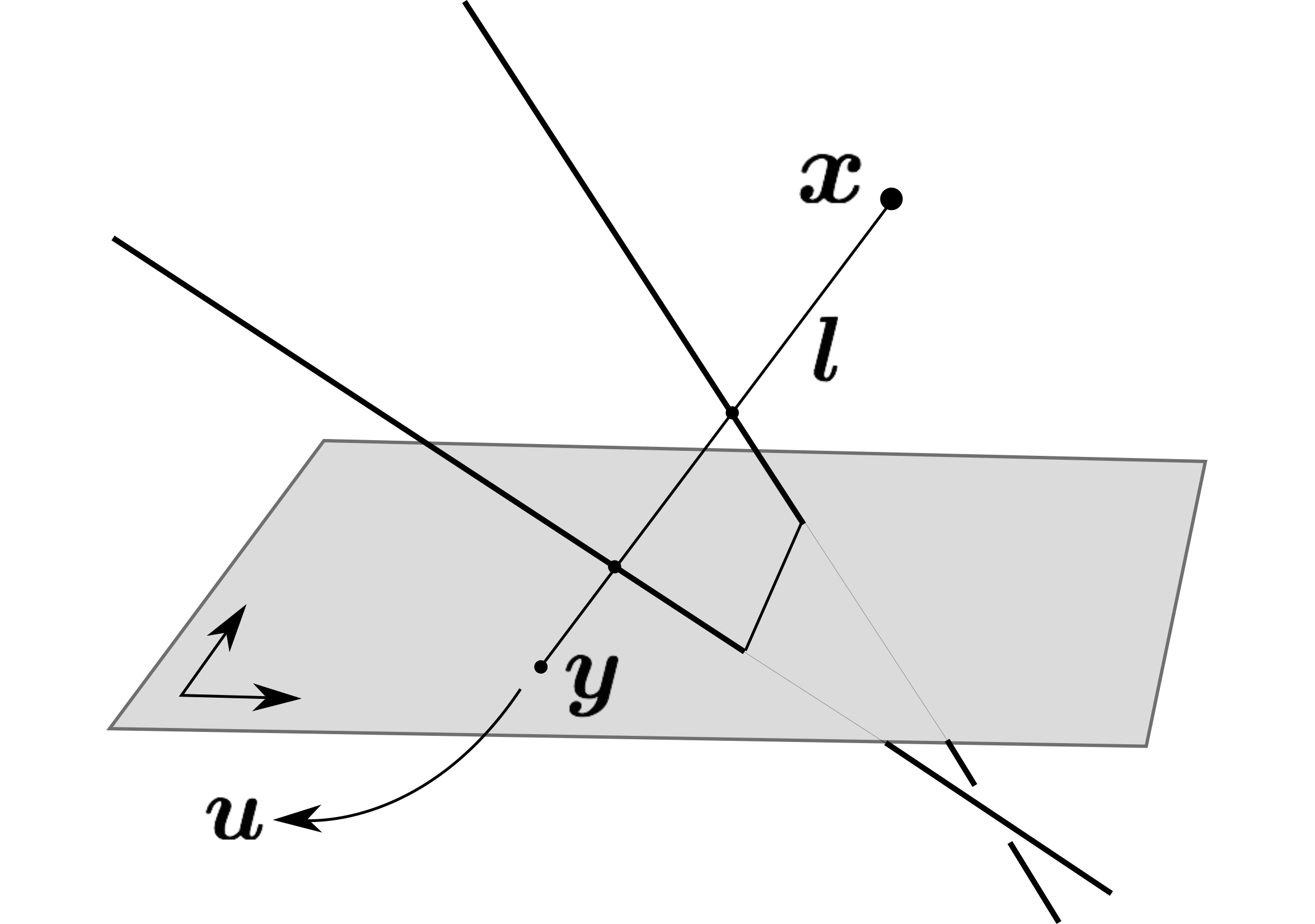
Figure 1: A general camera associates a scene point $x$ with a visual ray $l$, then maps the ray $l$ to its intersection $y$ with some retinal plane $\pi$, and finally uses a projective coordinate system on $\pi$ to express $y$ as a point $u$ in $\mathbb{P}^{2}$.

In particular, by introducing the notion of “primitive” camera model as the orbit of a camera under the action of projective, affine, similarity, and euclidean transformations, we can generalize many classical attributes of pinhole projections, such as intrinsic coordinates and calibration matrices. Our methodology applies to arbitrary (rational) cameras, but it is illustrated concretely by an in-depth study of two-slit cameras [2, 7, 13, 27], which we describe using a pair of linear $2\times 4$ projection matrices. This simple form allows us to describe models for the corresponding primitive cameras, to introduce intrinsic parameters with a clear geometric meaning, and to define an epipolar tensor characterizing two-view correspondences. In turn, this leads to new algorithms for structure from motion and self-calibration.

1.1 Background

Pinhole (or central) perspective has served since the XV${}^{\text{th}}$ Century as an effective model of physical imaging systems, from the camera obscura and the human eye to the daguerreotype and today’s digital photographic or movie cameras. Under this model, a scene point $x$ is first mapped onto the unique line $l$ joining $x$ to $c$, which is itself then mapped onto its intersection $y$ with some retinal plane $\pi$. All retinas are projectively equivalent, and thus the essential part of the imaging process is the map $\lambda_{L_{c}}:\mathbb{P}^{3}\setminus\mbox{\boldmath$c$}\rightarrow L_{c}$ associating a point with the corresponding visual ray in the bundle $L_{c}$ of all lines through the pinhole $c$ [17]. Similarly, many non-central cameras can be imagined (and actually constructed [21, 22, 25]) by replacing the line bundle $L_{c}$ with a more general family of lines. For example, Pajdla [14] and Batog et al. [2] have considered cameras that are associated with linear congruences, i.e., two-dimensional families of lines that obey linear constraints. This model applies two-slit [13, 24, 27], pushbroom [7], and pencil [26] cameras. For these devices, the projection can be described by a projective map $A$ so that each point $x$ is mapped to the line joining $x$ and $A\mbox{\boldmath$x$}$. Recently, a generalization of this model to non-linear congruences [10, 15] has been introduced by Ponce, Sturmfels and Trager [19]. They study algebraic properties of the essential map that associates scene points to the corresponding viewing rays, and provide a general framework for studying multi-view geometry in this setting. On the other hand, they do not focus on the auxiliary part of the imaging process, that associates viewing rays with image coordinates, leaving this map left unspecified as an arbitrary birational map from a congruence to $\mathbb{P}^{2}$. We provide in Section 2 the missing link with a concrete retinal plane and (pixel) coordinate systems, which is key for defining intrinsic parameters that have physical meaning, and for developing actual algorithms for multi-view reconstruction.

1.2 Contributions

From a theoretical standpoint: 1) we present a concrete embedding of the abstract rational cameras introduced in [19], deriving general direct and inverse projection formulas for these cameras, and 2) we introduce the notion of primitive camera models, that are orbits of rational cameras under the action of the projective, affine, and euclidean and similarity groups, and lead to the generalization familiar concepts such as intrinsic camera parameters. From a more concrete point of view, we use this model for an in-depth study of two-slit cameras [2, 13, 27]. Specifically, 1) we introduce a pair of calibration matrices, which generalize to our setting the familiar upper-triangular matrices associated with pinhole cameras, and can be identified with the orbits of two-slit cameras under similarity transforms; 2) we define the epipolar tensor, that encodes the projective geometry of a pair of two-slit cameras, and generalizes the traditional fundamental matrix; and 3) use these results to describe algorithms for structure from motion and self-calibration.

To improve readability, most proofs and technical material are deferred to the supplementary material.

1.3 Notation and elementary line geometry

Notation. We use bold letters for matrices and vectors ($\mbox{\boldmath$A$},\mbox{\boldmath$x$}$, $u$, etc.) and regular fonts for coordinates ($a_{i},x_{i},u_{i}$, etc.). Homogeneous coordinates are lowercase and indexed from one, and both points and planes are column vectors, e.g., $\mbox{\boldmath$x$}=(x_{1},x_{2},x_{3},x_{4})^{T}$, $\mbox{\boldmath$u$}=(u_{1},u_{2},u_{3})^{T}$. For projective objects, equality is always up to some scale factor. We identify $\mathbb{R}^{3}$ with points $(x_{1},x_{2},x_{3},1)^{T}$ in $\mathbb{P}^{3}$, and adopt the standard euclidean metric. We also use the natural hierarchy among projective transformations by the nested subgroups (dubbed from now on natural projective subgroups) formed by euclidean (orientation-preserving) transformations, similarities (euclidean transformations plus scaling), affine transformations, and projective ones. We will assume that the reader is familiar with their analytical form.

Line geometry. The set of all lines of $\mathbb{P}^{3}$ forms a four-dimensional variety, the Grassmannian of lines, denoted by $\text{Gr}(1,3)$. The line passing through two distinct points $x$ and $y$ in $\mathbb{P}^{3}$ can be represented using Plücker coordinates by writing $\mbox{\boldmath$l$}=(l_{41},l_{42},l_{43},l_{23},l_{31},l_{12})$ where $l_{ij}=x_{i}y_{j}-x_{j}y_{i}$. This defines a point in $\mathbb{P}^{5}$ that is independent of the choice of $x$ and $y$ along $l$. Moreover, the coordinates of any line $l$ satisfy the constraint $\mbox{\boldmath$l$}\cdot\mbox{\boldmath$l$}^{*}=0$, where $\mbox{\boldmath$l$}^{*}=(l_{23},l_{31},l_{12},l_{41},l_{42},l_{43})$ is the dual line for $l$. Conversely any point in $\mathbb{P}^{5}$ with this property represents a line, so $\text{Gr}(1,3)$ can be identified with a quadric hypersurface in $\mathbb{P}^{5}$. The join ($\vee$) and meet ($\wedge$) operators are used to indicate intersection and span of linear spaces (points, lines, planes). For example, $\mbox{\boldmath$x$}\vee\mbox{\boldmath$y$}$ denotes the unique line passing through $x$ and $y$. To give analytic formulae for these operators, it useful to introduce the primal and dual Plücker matrices for a line $l$: these are defined respectively as $\mbox{\boldmath$L$}=\mbox{\boldmath$x$}\mbox{\boldmath$y$}^{T}-\mbox{\boldmath$y$}\mbox{\boldmath$x$}^{T}$ and $\mbox{\boldmath$L$}^{*}=\mbox{\boldmath$u$}\mbox{\boldmath$v$}^{T}-\mbox{\boldmath$v$}\mbox{\boldmath$u$}^{T}$, where $\mbox{\boldmath$x$},\mbox{\boldmath$y$}$ are any two points on $l$, and $\mbox{\boldmath$u$},\mbox{\boldmath$v$}$ are any two planes containing $l$ (so $\mbox{\boldmath$l$}=\mbox{\boldmath$x$}\vee\mbox{\boldmath$y$}=\mbox{\boldmath$u$}\wedge\mbox{\boldmath$v$}$). With these definitions, the join $\mbox{\boldmath$l$}\vee\mbox{\boldmath$z$}$ of $l$ with a point $z$ is the plane with coordinates $\mbox{\boldmath$L$}^{*}\mbox{\boldmath$z$}$, while the meet $\mbox{\boldmath$l$}\wedge\mbox{\boldmath$w$}$ with a plane $w$ is the point with coordinates $L$$w$.

2 A physical model for rational cameras

For convenience of the reader, we briefly recall in Section 2.1 some results from [19]. We then proceed to new results in Sections 2.2 and 2.3.

2.1 Cameras and line congruences

Congruences. A line congruence is a two-dimensional family of lines in $\mathbb{P}^{3}$, or a surface in $\text{Gr}(1,3)$ [10]. Since a general camera produces a two-dimensional image, the set of viewing rays captured by the imaging device will form a congruence. We will only consider algebraic congruences that are defined by polynomial equations in $\text{Gr}(1,3)$. Every such congruence $L$ is associated with two non-negative integers $(\alpha,\beta)$: the order $\alpha$ is the number of rays in $L$ that pass through a generic point of $\mathbb{P}^{3}$, while the class $\beta$ is the number of lines in $L$ that lie in a generic plane. The pair $(\alpha,\beta)$ is the bidegree of the congruence. The set of points that do not belong to $\alpha$ distinct lines is the focal locus $F(L)$.

Geometric rational cameras. Order one congruences (or $(1,\beta)$-congruences) are a natural geometric model for most imaging systems [1, 2, 17]. Indeed, a $(1,\beta)$-congruence $L$ defines a rational map $\lambda_{L}:\mathbb{P}^{3}\dashrightarrow{\rm Gr}(1,3)$ associating a generic point $x$ in $\mathbb{P}^{3}$ with the unique $\lambda_{L}(\mbox{\boldmath$x$})$ line in $L$ that contains $x$. All possible maps of this form are described in [19]. The Plücker coordinates of a line $\lambda_{L}(\mbox{\boldmath$x$})$ are homogeneous polynomials (or forms) of degree $\beta+1$ in the coordinates of $x$. For example, a family of $(1,\beta)$-congruences are defined by an algebraic curve $\gamma$ of degree $\beta$ and a line $\delta$ intersecting $\gamma$ in $\beta-1$ points [15]. Its rays are the common transversals to $\gamma$ and $\delta$. The mapping $\lambda_{L}:\mathbb{P}^{3}\dashrightarrow\text{Gr}(1,3)$ can be expressed, using appropriate coordinates of $\mathbb{P}^{3}$, by

$$\small\lambda_{L}(\mbox{\boldmath$x$})=\left[\begin{matrix}x_{1}\\ x_{2}\\ x_{3}\\ x_{4}\end{matrix}\right]\vee\left[\begin{matrix}x_{1}f(x_{1},x_{2})\\ x_{2}f(x_{1},x_{2})\\ g(x_{1},x_{2})\\ h(x_{1},x_{2})\end{matrix}\right],$$ (1)

where $f$, $g$ and $h$ are respectively forms of degree $\beta-1$, $\beta$ and $\beta$. The remaining $(1,\beta)$-congruences for $\beta>0$ correspond to degenerations of this case, or to transversals to twisted cubics. These can be parameterized in a similar manner [19].

Photographic rational cameras. Composing $\lambda_{L}:\mathbb{P}^{3}\dashrightarrow\text{Gr}(1,3)$ with an arbitrary birational map $\nu:L\dashrightarrow\mathbb{P}^{2}$ determines a map $\psi=\nu\circ\lambda_{L}:\mathbb{P}^{3}\dashrightarrow\mathbb{P}^{2}$, which is taken as the definition of a general “photographic” rational camera in [19]. Although this model leads to effective formulations of multi-view constraints, it is abstract, with no explicit link between $\mbox{\boldmath$u$}=\psi(\mbox{\boldmath$x$})$ and the actual image point where the ray $\lambda_{L}(\mbox{\boldmath$x$})$ intersects the sensing array.

2.2 Rational cameras with retinal planes

In this paper, we adapt the framework from [19] for studying physical instances of photographic cameras. We will refer to the map $\lambda_{L}$ defined by a $(1,\beta)$-congruence $L$ as the essential part of the imaging process (or an “essential camera” for short). The auxiliary part of the process requires choosing a retinal plane $\pi$ in $\mathbb{P}^{3}$. This determines a map $\mu_{\mbox{\boldmath$\pi$}}:L\dashrightarrow\mbox{\boldmath$\pi$}$ that associates any ray $l$ in $L$ not lying in $\pi$ with its intersection $\mbox{\boldmath$y$}=\mbox{\boldmath$l$}\wedge\mbox{\boldmath$\pi$}$ with that plane. For a generic choice of $\pi$, this map is not defined on $\beta$ lines, since $\beta$ lines from $L$ will lie on $\pi$ (recall the definition of $\beta$ from Section 2.1). Together, $\lambda_{L}$ and $\mu_{\mbox{\boldmath$\pi$}}$ (or, equivalently, $L$ and $\pi$) define a mapping $\mu_{\mbox{\boldmath$\pi$}}\circ\lambda_{L}:\mathbb{P}^{3}\dashrightarrow\mbox{\boldmath$\pi$}$ that can be taken as a definition of a geometric rational camera. Finally, an analytic counterpart of this model is obtained by picking a coordinate system $(\pi)$ on $\pi$, that corresponds to the pixel grid where radiometric measurements are obtained. Representing $(\pi)$ as a $4\times 3$ matrix $\mbox{\boldmath$Y$}=[\mbox{\boldmath$y$}_{1},\mbox{\boldmath$y$}_{2},\mbox{\boldmath$y$}_{3}]$, where columns correspond to basis points, the coordinates $u$ in $\mathbb{P}^{2}$ of any point $y$ on $\pi$ are given by $\mbox{\boldmath$u$}=\mbox{\boldmath$Y$}^{\dagger}\mbox{\boldmath$y$}$, where $\mbox{\boldmath$Y$}^{\dagger}$ is a $3\times 4$ matrix in the three-parameter set of pseudoinverses of $Y$ (see for example [17]). Note that both $\mu_{\mbox{\boldmath$\pi$}}$ and $\mbox{\boldmath$Y$}^{\dagger}$ are linear, and in fact a simple calculation shows that $\mbox{\boldmath$N$}=\mbox{\boldmath$Y$}^{\dagger}\circ\mu_{\mbox{\boldmath$\pi$}}$ is described by the $3\times 6$ matrix

$$\small\mbox{\boldmath$N$}=\mbox{\boldmath$Y$}^{\dagger}\circ\mu_{\mbox{\boldmath$\pi$}}=\left[\begin{matrix}(\mbox{\boldmath$y$}_{2}\vee\mbox{\boldmath$y$}_{3})^{*T}\\ (\mbox{\boldmath$y$}_{3}\vee\mbox{\boldmath$y$}_{1})^{*T}\\ (\mbox{\boldmath$y$}_{1}\vee\mbox{\boldmath$y$}_{2})^{*T}\end{matrix}\right].$$ (2)

This expression does not depend on $L$: it represents a linear map $\mathbb{P}^{5}\dashrightarrow\mathbb{P}^{2}$ that associates a generic line $l$ in $\mathbb{P}^{3}$ with the coordinates $u$ in $\mathbb{P}^{2}$ of its intersection with $\pi$.

Example 1.

Consider the plane $\mbox{\boldmath$\pi$}=\{x_{3}-x_{4}=0\}$ in $\mathbb{P}^{3}$, equipped with the reference frame given by $\mbox{\boldmath$y$}_{1}=(1,0,0,0)^{T}$, $\mbox{\boldmath$y$}_{2}=(0,1,0,0)^{T}$, $\mbox{\boldmath$y$}_{3}=(0,0,1,1)^{T}$ (with fixed relative scale). The matrix $N$ takes in this case the form

$$\small\mbox{\boldmath$N$}=\begin{bmatrix}1&0&0&0&-1&0\\ 0&1&0&1&0&0\\ 0&0&1&0&0&0\end{bmatrix}.$$ (3)

The null space of the corresponding linear projection is $\{p_{41}-p_{31}=p_{42}+p_{23}=p_{43}=0\}$, which characterizes lines contained in $\pi$. $\diamondsuit$

In summary, a complete analytical model of a physical photographic rational camera is a map $\psi:\mathbb{P}^{3}\dashrightarrow\mathbb{P}^{2}$ that is the composition of the essential map $\lambda_{L}:\mathbb{P}^{3}\dashrightarrow\text{Gr}(1,3)$, associated with a $(1,\beta)$-congruence $L$, and the linear map $N$ of (2):

$$\small\mbox{\boldmath$x$}\mapsto\mbox{\boldmath$u$}=\psi(\mbox{\boldmath$x$})=\mbox{\boldmath$N$}\lambda_{L}(\mbox{\boldmath$x$}).$$ (4)

By construction, the coordinates of $\psi(\mbox{\boldmath$x$})$ are forms of degree $\beta+1$ in $x$. One could of course define directly a rational camera in terms of such forms (and indeed rational cameras are commonly used in photogrammetry [9]). Note, however, that arbitrary rational maps do not, in general, define a camera, since the pre-image of a generic point $u$ in $\mathbb{P}^{2}$ should be a line. From (4) we also easily recover the inverse projection $\chi:\mathbb{P}^{2}\dashrightarrow\text{Gr}(1,3)$ mapping a point in $\mathbb{P}^{2}$ onto the corresponding viewing ray in $L$:

$$\small\mbox{\boldmath$u$}\mapsto\mbox{\boldmath$l$}=\chi(\mbox{\boldmath$u$})=\lambda_{L}(\mbox{\boldmath$Y$}\mbox{\boldmath$u$}).$$ (5)

The Plücker coordinates of $l$ are also forms of degree $\beta+1$ in $u$. Equation (5) can be used to define epipolar or multi-view constraints for point correspondences, since it allows one to express incidence constraints among viewing rays in terms of the corresponding image coordinates [22]. See also Section 4.

To conclude, let us point out that although a rational camera $\psi:\mathbb{P}^{3}\dashrightarrow\mathbb{P}^{2}$ was introduced in terms of a congruence $L$, a retinal plane $\pi$, and a projective reference frame on $\pi$, the retinal plane is often not (completely) determined given $\psi$. This is well known for pinhole cameras, and we will argue that a similar ambiguity arises for two-slit cameras. On the other hand, it is easy to see that the congruence $L$ and the global mapping $N$ can always be recovered from the analytic expression of the camera: the congruence $L$ is in fact determined by the pre-images $\psi^{-1}(\mbox{\boldmath$u$})$ under $\psi$ of points $u$ in $\mathbb{P}^{2}$, while $N$ is described by $\mbox{\boldmath$N$}(\psi^{-1}(\mbox{\boldmath$u$}))=\mbox{\boldmath$u$}$.

2.3 Primitive camera models

The orbit of a rational camera under the action of any of the four natural projective subgroups defined earlier is a family of cameras that are geometrically and analytically equivalent under the corresponding transformations. Each orbit will be called a primitive camera model for the corresponding subgroup, and we will attach to every such model, whenever appropriate and possible, a particularly simple analytical representative. A primitive camera model exhibits (analytical and geometric) invariants, that is, properties of all cameras in the same orbit that are preserved by the associated group of transformations. For example, the intrinsic parameters of a pinhole perspective camera are invariants for the corresponding euclidean primitive model; we will argue in the next section that this definition can in fact be applied for arbitrary rational cameras. Another familiar example is the projection of the absolute conic, which is an invariant for the similarity orbit of any imaging system. Indeed, the absolute conic, defined in any euclidean coordinate system by $\{x_{4}=x_{1}^{2}+x_{2}^{2}+x_{3}^{2}=0\}$, is fixed by all similarity transformations. This property is commonly used for the self-calibration of pinhole perspective cameras [12, 16, 18, 23] but it can be used for more general cameras as well (see Section 4).

To further illustrate these concepts, we describe classical primitive models for pinhole projections. We consider the standard pinhole projection $\psi(\mbox{\boldmath$x$})=(x_{1},x_{2},x_{3})^{T}$, associated with the $3\times 4$-matrix $[\text{Id}\,|\,\mbox{\boldmath$0$}]$. Its projective orbit consists of all linear projections $\mathbb{P}^{3}\dashrightarrow\mathbb{P}^{2}$, corresponding to $3\times 4$ matrices of full rank, so pinhole cameras form a primitive projective model. The affine orbit of $\psi$ is the family of finite cameras, i.e., cameras of the form $[\mbox{\boldmath$A$}\,|\,\mbox{\boldmath$b$}]$, where $A$ is a $3\times 3$ full-rank matrix. The orbit of $\psi$ under similarities or under euclidean transformations is the set of cameras of the form $[\mbox{\boldmath$R$}\,|\,\mbox{\boldmath$t$}]$ where $R$ is a rotation matrix. The euclidean and similarity orbits in this case coincide: this is of course related to the scale ambiguity in pictures taken with perspective pinhole cameras. The euclidean/similarity invariants of a finite camera can be expressed as entries of a $3\times 3$ upper-triangular calibration matrix $K$: this follows from the uniqueness of the RQ-decomposition $\mbox{\boldmath$A$}=\mbox{\boldmath$K$}\mbox{\boldmath$R$}$. Primitive models for cameras “at infinity” include affine, scaled orthographic, and orthographic projections: these are defined by the orbits under natural projective groups of $\psi^{\prime}(\mbox{\boldmath$x$})=(x_{1},x_{2},x_{4})^{T}$. Here the similarity and euclidean orbits are different (indeed, orthographic projections preserve distances). The intrinsic parameters can be expressed as entries of a $2\times 2$ calibration matrix (see [8, Sec. 6.3]).

The remaining part of the paper focuses on a particular class of rational cameras, namely two-slit cameras, for which the general concepts introduced above can be easily applied. Two-slit cameras correspond in fact to congruences of class $\beta=1$, so they can be viewed as the “simplest” rational cameras after pinhole projections.

3 Two-slit cameras: a case study

Two-slit cameras [3, 7, 13, 24, 27] record viewing rays that are the transversals to two fixed skew lines (the slits). The bidegree of the associated congruence is $(1,1)$, since a generic plane will contain exactly one transversal to the slits, namely the line joining the points where the slits intersect the plane. This type of congruence is the intersection of $\text{Gr}(1,3)$ with a $3$-dimensional linear space in $\mathbb{P}^{5}$ [2]. The map $\lambda_{L}$ associated with the slits $\mbox{\boldmath$l$}_{1},\mbox{\boldmath$l$}_{2}$ is

$$\small\mbox{\boldmath$x$}\mapsto\mbox{\boldmath$l$}=(\mbox{\boldmath$x$}\vee\mbox{\boldmath$l$}_{1})\wedge(\mbox{\boldmath$x$}\vee\mbox{\boldmath$l$}_{2}).$$ (6)

We now fix a retinal plane $\pi$ equipped with the coordinate system defined by $\mbox{\boldmath$Y$}=[\mbox{\boldmath$y$}_{1},\mbox{\boldmath$y$}_{2},\mbox{\boldmath$y$}_{3}]$. A rational camera $\psi:\mathbb{P}^{3}\dashrightarrow\mathbb{P}^{2}$ is obtained by composing (6) with the $3\times 6$ matrix $N$ as in (2). A simple calculation shows that the resulting map can be written compactly as

$$\small\mbox{\boldmath$x$}\mapsto\mbox{\boldmath$u$}=\begin{bmatrix}\mbox{\boldmath$x$}^{T}\mbox{\boldmath$P$}_{1}^{*}\mbox{\boldmath$S$}_{1}\mbox{\boldmath$P$}_{2}^{*}\mbox{\boldmath$x$}\\ \mbox{\boldmath$x$}^{T}\mbox{\boldmath$P$}_{1}^{*}\mbox{\boldmath$S$}_{2}\mbox{\boldmath$P$}_{2}^{*}\mbox{\boldmath$x$}\\ \mbox{\boldmath$x$}^{T}\mbox{\boldmath$P$}_{1}^{*}\mbox{\boldmath$S$}_{3}\mbox{\boldmath$P$}_{2}^{*}\mbox{\boldmath$x$}\\ \end{bmatrix},$$ (7)

where $\mbox{\boldmath$P$}_{1}^{*},\mbox{\boldmath$P$}_{2}^{*}$ are the dual Plücker matrices associated with the slits $\mbox{\boldmath$l$}_{1},\mbox{\boldmath$l$}_{2}$, while $\mbox{\boldmath$S$}_{1},\mbox{\boldmath$S$}_{2},\mbox{\boldmath$S$}_{3}$ are Plücker matrices for $\mbox{\boldmath$y$}_{2}\vee\mbox{\boldmath$y$}_{3}$, $\mbox{\boldmath$y$}_{3}\vee\mbox{\boldmath$y$}_{1}$, $\mbox{\boldmath$y$}_{1}\vee\mbox{\boldmath$y$}_{2}$ respectively [3, 27].

Example 2.

Let us fix the slits to be the lines $\mbox{\boldmath$l$}_{1}=\{x_{1}=x_{3}=0\},\mbox{\boldmath$l$}_{2}=\{x_{2}=x_{3}+x_{4}=0\}$. The corresponding essential map $\mathbb{P}^{3}\dashrightarrow\text{Gr}(1,3)$ is given by

$$\small\small\lambda(\mbox{\boldmath$x$})=(x_{1}(x_{3}+x_{4}),x_{2}x_{3},x_{3}(x_{3}+x_{4}),x_{2}x_{3},0,-x_{1}x_{2})^{T}$$ (8)

Composing with the projection $N$ in Example 1, we obtain the formula for a rational camera with slits $\mbox{\boldmath$l$}_{1},\mbox{\boldmath$l$}_{2}$:

$$\small\small\mbox{\boldmath$u$}=\psi(\mbox{\boldmath$x$})=(x_{1}(x_{3}+x_{4}),2x_{2}x_{3},x_{3}(x_{3}+x_{4}))^{T}$$ (9)

The same expression can be deduced from (7). $\diamondsuit$

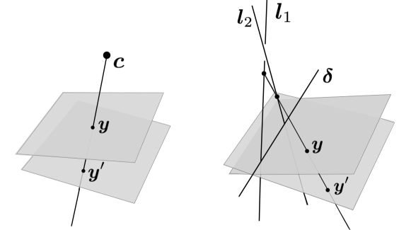
Figure 2: Left: A pinhole $c$ induces a homography between any two retinal planes not containing $c$. Right: Two skew lines $\mbox{\boldmath$l$}_{1},\mbox{\boldmath$l$}_{2}$ induce a homography between planes intersecting at a transversal $\delta$ to $\mbox{\boldmath$l$}_{1},\mbox{\boldmath$l$}_{2}$.

It is noted in [3, 27] that using a different retinal plane $\pi$ in (7) corresponds, in general, to composing the rational camera $\psi:\mathbb{P}^{3}\dashrightarrow\mathbb{P}^{2}$ with a quadratic change of image coordinates $\mathbb{P}^{2}\dashrightarrow\mathbb{P}^{2}$. However, this transformation is in fact linear when $\pi$ and $\mbox{\boldmath$\pi$}^{\prime}$ intersect along a transversal to the slits. This follows from the following property:

Lemma 1.

Let $\mbox{\boldmath$l$}_{1},\mbox{\boldmath$l$}_{2}$ be two skew lines in $\mathbb{P}^{3}$. For any point $x$ not on the these lines, we indicate with $\lambda(\mbox{\boldmath$x$})$ the unique transversal to ${\mbox{\boldmath$l$}_{1},\mbox{\boldmath$l$}_{2}}$ passing through $x$. If $\pi$ and $\mbox{\boldmath$\pi$}^{\prime}$ are two planes intersecting at a line $\delta$ that intersects $\mbox{\boldmath$l$}_{1}$ and $\mbox{\boldmath$l$}_{2}$, then the map $f:\mbox{\boldmath$\pi$}\dashrightarrow\mbox{\boldmath$\pi$}^{\prime}$ defined, for points $y$ not on $\delta$, as

$$\small f(\mbox{\boldmath$y$})=\lambda(\mbox{\boldmath$y$})\wedge\mbox{\boldmath$\pi$}^{\prime},$$ (10)

can be extended to a homography between $\pi$ and $\mbox{\boldmath$\pi$}^{\prime}$.

This Lemma also implies that two retinal planes that intersect at a transversal to the slits can define the same rational camera (using appropriate coordinate systems). Note the similarity with the traditional pinhole case, where the choice of the retinal plane is completely irrelevant since the pinhole $c$ induces a homography between any planes $\mbox{\boldmath$\pi$},\mbox{\boldmath$\pi$}^{\prime}$ not containing $c$. See Figure 2.

3.1 A projective model using linear projections

Contrary to the case of pinhole cameras, two-slit cameras of the form (7) are not all projectively equivalent. This can be argued by noting that the coordinates $\mbox{\boldmath$u$}_{1},\mbox{\boldmath$u$}_{2}$ in $\mathbb{P}^{2}$ of the points $\mbox{\boldmath$y$}_{1}=\mbox{\boldmath$l$}_{1}\wedge\mbox{\boldmath$\pi$}$, $\mbox{\boldmath$y$}_{2}=\mbox{\boldmath$l$}_{2}\wedge\mbox{\boldmath$\pi$}$ (the intersections of the slits with the retinal planes) are always preserved by projective transformations of $\mathbb{P}^{3}$. For Batog et al. [1, 2], the coordinates $\mbox{\boldmath$u$}_{1},\mbox{\boldmath$u$}_{2}$ are “intrinsic parameters” of the camera; indeed, they are projective intrinsics (i.e., invariants) of a two-slit device. Batog et al. also argue that choosing the points $\mbox{\boldmath$y$}_{1}$, $\mbox{\boldmath$y$}_{2}$ as points in the projective basis on $\pi$ leads to simplified analytic expressions for the projection. Here, we develop this idea further, and observe that any two-slit camera with this kind of coordinate system can always be described by a pair of linear projections. More precisely, for any retinal plane $\pi$, let us fix a coordinate system $\mbox{\boldmath$Y$}=[\mbox{\boldmath$y$}_{1},\mbox{\boldmath$y$}_{2},\mbox{\boldmath$y$}_{3}]$ where $\mbox{\boldmath$y$}_{1}=\mbox{\boldmath$l$}_{2}\wedge\mbox{\boldmath$\pi$}$, $\mbox{\boldmath$y$}_{2}=\mbox{\boldmath$l$}_{1}\wedge\mbox{\boldmath$\pi$}$ and $\mbox{\boldmath$y$}_{3}$ is arbitrary: in this case, a straightforward computation shows that (7) reduces to

$${\small\mbox{\boldmath$x$}\mapsto\left[\begin{matrix}u_{1}\\ u_{2}\\ u_{3}\end{matrix}\right]=\left[\begin{matrix}(\mbox{\boldmath$p$}_{1}^{T}\mbox{\boldmath$x$})\,\,(\mbox{\boldmath$q$}_{2}^{T}\mbox{\boldmath$x$})\\ (\mbox{\boldmath$p$}_{2}^{T}\mbox{\boldmath$x$})\,\,(\mbox{\boldmath$q$}_{1}^{T}\mbox{\boldmath$x$})\\ (\mbox{\boldmath$p$}_{2}^{T}\mbox{\boldmath$x$})\,\,(\mbox{\boldmath$q$}_{2}^{T}\mbox{\boldmath$x$})\end{matrix}\right]=\left[\begin{matrix}\mbox{\boldmath$p$}_{1}^{T}\mbox{\boldmath$x$}/\mbox{\boldmath$p$}_{2}^{T}\mbox{\boldmath$x$}\\ \mbox{\boldmath$q$}_{1}^{T}\mbox{\boldmath$x$}/\mbox{\boldmath$q$}_{2}^{T}\mbox{\boldmath$x$}\\ 1\end{matrix}\right],}$$ (11)

where $\mbox{\boldmath$p$}_{1}=(\mbox{\boldmath$l$}_{1}\vee\mbox{\boldmath$y$}_{3})$, $\mbox{\boldmath$p$}_{2}=-(\mbox{\boldmath$l$}_{1}\vee\mbox{\boldmath$y$}_{1})$, $\mbox{\boldmath$q$}_{1}=(\mbox{\boldmath$l$}_{2}\vee\mbox{\boldmath$y$}_{3})$, $\mbox{\boldmath$q$}_{2}=-(\mbox{\boldmath$l$}_{2}\vee\mbox{\boldmath$y$}_{2})$ are vectors representing planes in $\mathbb{P}^{3}$. It is easy to see that this quadratic map can be described using two linear maps $\mathbb{P}^{3}\dashrightarrow\mathbb{P}^{1}$, namely

$$\small\mbox{\boldmath$x$}\mapsto\left[\begin{matrix}u_{1}\\ u_{3}\end{matrix}\right]=\left[\begin{matrix}\mbox{\boldmath$p$}_{1}^{T}\mbox{\boldmath$x$}\\ \mbox{\boldmath$p$}_{2}^{T}\mbox{\boldmath$x$}\end{matrix}\right]=\mbox{\boldmath$A$}_{1}\mbox{\boldmath$x$},\,\,\mbox{\boldmath$x$}\mapsto\left[\begin{matrix}u_{2}\\ u_{3}\end{matrix}\right]=\left[\begin{matrix}\mbox{\boldmath$q$}_{1}^{T}\mbox{\boldmath$x$}\\ \mbox{\boldmath$q$}_{2}^{T}\mbox{\boldmath$x$}\end{matrix}\right]=\mbox{\boldmath$A$}_{2}\mbox{\boldmath$x$}.$$ (12)

In other words, (11) determines the $2\times 4$ matrices $\mbox{\boldmath$A$}_{1}$ and $\mbox{\boldmath$A$}_{2}$ up to two scale factors, and vice-versa. Since applying a projective transformation to $x$ in (11) corresponds to a matrix multiplication applied to both $\mbox{\boldmath$A$}_{1}$ and $\mbox{\boldmath$A$}_{2}$, we easily deduce that every pair of $2\times 4$-matrices of full rank and with disjoint null-spaces corresponds to a two-slit camera, and that all these cameras are projectively equivalent. The two $2\times 4$ matrices for a two-slit camera are analogues of the $3\times 4$ matrix representing a pinhole camera: for example, the slits are associated with the null-spaces of these two matrices. For two given projection matrices, the retinal plane may be any plane containing the line $\{\mbox{\boldmath$p$}_{2}^{T}\mbox{\boldmath$x$}=\mbox{\boldmath$q$}_{2}^{T}\mbox{\boldmath$x$}=0\}$: this is the line through $\mbox{\boldmath$y$}_{1}$ and $\mbox{\boldmath$y$}_{2}$, and is the locus of points where the projection is not defined. This completely describes a primitive projective model with $7+7=14$ degrees of freedom. More precisely, there are $8$ degrees of freedom corresponding to the choice of the slits, $2$ for the intersection points of the retinal plane with the slits, and $4$ for the choice of coordinates on the plane (since two basis points are constrained).

In the remainder of the paper, we will always assume that a two-slit photographic camera is of the form (11). This is equivalent to knowing the “projective intrinsic parameters” [2], namely the coordinates of $\mbox{\boldmath$l$}_{1}\wedge\mbox{\boldmath$\pi$}$, $\mbox{\boldmath$l$}_{2}\wedge\mbox{\boldmath$\pi$}$. We will also identify a camera with its two associated projection matrices.

Example 3.

The two-slit projection from Example 2 is of the form (11) with

$$\small\mbox{\boldmath$A$}_{1}=\begin{bmatrix}1&0&0&0\\ 0&0&1&0\end{bmatrix},\mbox{\boldmath$A$}_{2}=\begin{bmatrix}0&2&0&0\\ 0&0&1&1\end{bmatrix}.$$ (13)

The retinal plane belongs to the pencil of planes containing $\{x_{3}=x_{3}+x_{4}=0\}$, i.e., it is a plane of the form $x_{3}-dx_{4}=0$. The choice $d=1$ is natural since points of the form $[x_{1},x_{2},1,1]$ are mapped to $[x_{1},x_{2},1]$. $\diamondsuit$

3.2 Orbits and calibration matrices

Using the linear model introduced above, we can easily describe affine, similarity, and euclidean orbits for two-slit cameras. For example, the affine orbit of the device in (9), (13) corresponds to

$$\small\mbox{\boldmath$A$}_{1}=\begin{bmatrix}\mbox{\boldmath$m$}_{1}^{T}&t_{1}\\ \mbox{\boldmath$m$}_{3}^{T}&t_{3}\end{bmatrix},\mbox{\boldmath$A$}_{2}=\begin{bmatrix}\mbox{\boldmath$m$}_{2}^{T}&t_{2}\\ \mbox{\boldmath$m$}_{3}^{T}&t_{4}\end{bmatrix},$$ (14)

where $\mbox{\boldmath$m$}_{i}$ are arbitrary $3$-vectors. This is the family of two-slit cameras where the retinal plane is parallel to the slits: indeed, although this plane is not completely determined, it is constrained to contain the line $\{[\mbox{\boldmath$m$}_{3}^{T},t_{3}]\mbox{\boldmath$x$}=[\mbox{\boldmath$m$}_{3}^{T},t_{4}]\mbox{\boldmath$x$}=0\}$, that intersects both slits. We will refer to (14) as a parallel two-slit camera. These cameras form an affine model with $12$ degrees of freedom.

We now consider the family of (euclidean) parallel cameras of the form

$$\small\mbox{\boldmath$A$}_{1}=\begin{bmatrix}1&0&0&0\\ 0&0&1&0\end{bmatrix},\,\,\mbox{\boldmath$A$}_{2}=\begin{bmatrix}2\cos\theta&2\sin\theta&0&0\\ 0&0&1&d\end{bmatrix}.$$ (15)

for $d\neq 0$ and $0<\theta<2\pi$ (and $\theta\neq\pi$). The slits for this camera are at an angle of $\theta$ and distance $d$. Note that (9) is of this form, with $\theta=\pi/2$ and $d=1$.

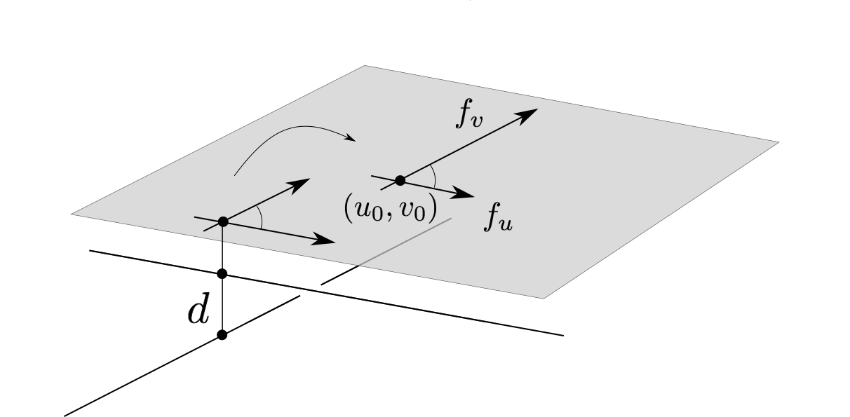
Figure 3: Physical interpretation of the entries the calibration matrices for parallel two-slit cameras: the parameters $f_{u},f_{v},u_{0},v_{0}$ describe the change of retinal plane coordinates, with respect to some camera in the euclidean orbit of (15).

Using (15) as a family of canonical euclidean devices, we can introduce expressions for the “intrinsic parameters” of two-slit cameras.

Proposition 1.

If $\mbox{\boldmath$A$}_{1}$, $\mbox{\boldmath$A$}_{2}$ describe a parallel two-slit camera (14), then we can uniquely write

$$\small\mbox{\boldmath$A$}_{1}=\mbox{\boldmath$K$}_{1}\begin{bmatrix}\mbox{\boldmath$r$}_{1}^{T}&t_{1}\\ \mbox{\boldmath$r$}_{3}^{T}&t_{3}\end{bmatrix},\,\,\mbox{\boldmath$A$}_{2}=\mbox{\boldmath$K$}_{2}\begin{bmatrix}\mbox{\boldmath$r$}_{2}^{T}&t_{2}\\ \mbox{\boldmath$r$}_{3}^{T}&t_{4}\end{bmatrix},$$ (16)

where $\mbox{\boldmath$K$}_{1}$ and $\mbox{\boldmath$K$}_{2}$ are upper-triangular $2\times 2$ matrices defined up to scale with positive elements along the diagonal, and $\mbox{\boldmath$r$}_{1},\mbox{\boldmath$r$}_{2},\mbox{\boldmath$r$}_{3}$ are unit vectors, with $\mbox{\boldmath$r$}_{3}$ orthogonal to both $\mbox{\boldmath$r$}_{1},\mbox{\boldmath$r$}_{2}$. Here, $\theta={\rm arccos}(\mbox{\boldmath$r$}_{1}\cdot\mbox{\boldmath$r$}_{2})$ is the angle between the slits, and $|t_{4}-t_{3}|$ is the distance between the slits. Moreover, if the matrices $\mbox{\boldmath$K$}_{1}$ and $\mbox{\boldmath$K$}_{2}$ are written as

$$\small\mbox{\boldmath$K$}_{1}=\begin{bmatrix}f_{u}&u_{0}\\ 0&1\end{bmatrix},\mbox{\boldmath$K$}_{2}=\begin{bmatrix}2f_{v}&v_{0}\\ 0&1\end{bmatrix},$$ (17)

then $f_{u},f_{v}$ can be interpreted as “magnifications” in the $u$ and $v$ directions, and $(u_{0},v_{0})$ as the position of the “principal point”. See Figure 3.

The parameters $\theta$ and $d$, and the matrices $\mbox{\boldmath$K$}_{1}$ and $\mbox{\boldmath$K$}_{2}$ are clearly invariant under euclidean transformations. Moreover, within the parallel model (14), two cameras belong to the same euclidean orbit if and only if all of their parameters are the same. In fact, the $12$ degrees of freedom of a parallel camera are split into $6$ corresponding to the “intrinsics” $\theta$, $d$, $\mbox{\boldmath$K$}_{1}$ and $\mbox{\boldmath$K$}_{2}$, and $6$ for the “extrinsic” action of euclidean motion. Compared to the traditional intrinsic parameters for pinhole cameras, we note the absence of a term corresponding to the “skewness” of the image reference frame. Indeed, the angle between the two axes must be the same as the angle between the slits, as a consequence of the “intrinsic coordinate system” (the principal directions correspond in fact to the fixed basis points $\mbox{\boldmath$y$}_{1},\mbox{\boldmath$y$}_{2}$ on the retinal plane). On the other hand, $\theta$ and $d$ do not have an analogue for pinhole cameras. We will sometimes refer to $d$ and $\theta$ as the “3D” intrinsic parameters, since we distinguish them from the “analytic” intrinsic parameters, that are entries of the calibration matrices $\mbox{\boldmath$K$}_{1},\mbox{\boldmath$K$}_{2}$, and differentiate (euclidean orbits of) cameras only based on analytic part of their mapping. We also point out that for two-slit cameras in (16), the euclidean orbit and the similarity orbit do not coincide: this implies that when the intrinsic parameters are known, some information on the scale of a scene can be inferred from a photograph [22].

Pushbroom cameras. Pushbroom cameras are degenerate class of projective two-slit cameras, in which one of the slits lies on the plane at infinity [3]. This is quite similar to the class affine cameras for perspective projections. Pushbrooms are handled by our projective model (11), but not by our affine one (14), where both slits are necessarily finite. We thus introduce another affine model, namely

$$\small\mbox{\boldmath$A$}_{1}=\begin{bmatrix}\mbox{\boldmath$m$}_{1}^{T}&t_{1}\\ \mbox{\boldmath$0$}&1\end{bmatrix},\,\,\mbox{\boldmath$A$}_{2}=\begin{bmatrix}\mbox{\boldmath$m$}_{2}^{T}&t_{2}\\ \mbox{\boldmath$m$}_{3}^{T}&t_{3}\end{bmatrix},$$ (18)

where $\mbox{\boldmath$m$}_{1},\mbox{\boldmath$m$}_{2},\mbox{\boldmath$m$}_{3}$ are arbitrary $3$-vectors. All such cameras are equivalent up to affine transformations, so this describes an affine model with $11$ degrees of freedom. The corresponding rational cameras can be written as

$$\small\mbox{\boldmath$x$}\mapsto\left([\mbox{\boldmath$m$}_{1}^{T},t_{1}]\mbox{\boldmath$x$},\frac{[\mbox{\boldmath$m$}_{2}^{T},t_{2}]\mbox{\boldmath$x$}}{[\mbox{\boldmath$m$}_{3}^{T},t_{3}]\mbox{\boldmath$x$}},1\right)^{T}.$$ (19)

This coincides with the linear pushbroom model proposed by Hartley and Gubta [7], who identify (19) with the $3\times 4$ matrix with rows $[\mbox{\boldmath$m$}_{1}^{T},t_{1}],[\mbox{\boldmath$m$}_{2}^{T},t_{2}],[\mbox{\boldmath$m$}_{3}^{T},t_{3}]$.

Let us now consider a family of affine pushbroom cameras of the form

$$\small\begin{bmatrix}\sin\theta&\cos\theta&0&0\\ 0&0&0&1\end{bmatrix}\begin{bmatrix}0&1&0&0\\ 0&0&1&0\end{bmatrix},$$ (20)

for $0<\theta<2\pi$ (and $\theta\neq\pi$). This represents a pushbroom camera where the direction of movement is at an angle $\theta$ with respect to the parallel scanning planes. We use this family of canonical devices to define calibration matrices and intrinsic parameters.

Proposition 2.

Let $\mbox{\boldmath$A$}_{1},\mbox{\boldmath$A$}_{2}$ define a pushbroom camera as in (18), and let us also assume that $\mbox{\boldmath$m$}_{1}$ and $\mbox{\boldmath$m$}_{3}$ are orthogonal. We can uniquely write

$$\small\mbox{\boldmath$A$}_{1}=\mbox{\boldmath$K$}_{1}\begin{bmatrix}\mbox{\boldmath$r$}_{1}^{T}&t_{1}\\ \mbox{\boldmath$0$}&1\end{bmatrix},\mbox{\boldmath$A$}_{2}=\mbox{\boldmath$K$}_{2}\begin{bmatrix}\mbox{\boldmath$r$}_{2}^{T}&t_{2}\\ \mbox{\boldmath$r$}_{3}^{T}&t_{3}\end{bmatrix}.$$ (21)

where $\mbox{\boldmath$K$}_{1}={\rm diag}(1/v,1)$, $\mbox{\boldmath$K$}_{2}=\begin{bmatrix}f&u\\ 0&1\end{bmatrix}$ (with positive $v$ and $f$) and $\mbox{\boldmath$r$}_{1},\mbox{\boldmath$r$}_{2},\mbox{\boldmath$r$}_{3}$ are unit vectors, with $\mbox{\boldmath$r$}_{3}$ orthogonal to both $\mbox{\boldmath$r$}_{1},\mbox{\boldmath$r$}_{2}$. Here, $\theta={\rm arccos}(\mbox{\boldmath$r$}_{1}\cdot\mbox{\boldmath$r$}_{2})$ is the angle between the two slits (or between the direction of motion of the sensor and the parallel scanning planes). Moreover, $v$ can be interpreted as the speed of the sensor, and $f$ and $u$ as the magnification and the principal point of the 1D projection.

The entries $\mbox{\boldmath$K$}_{1},\mbox{\boldmath$K$}_{2}$ are the “analytic” intrinsic parameters of the pushbroom camera, while $\theta$ is a “3D” intrinsic parameter.

4 Two-slit cameras: algorithms

In this section, we apply our study of two-slit cameras to develop algorithms for structure from motion (SfM). The epipolar geometry of two-slit cameras will be described in terms of a $2\times 2\times 2\times 2$ epipolar tensor. Previously, image correspondences between two-slit cameras have been characterized using a $6\times 6$ [3], or a $4\times 4$ fundamental matrix [2]. The latter approach, due to Batog et al. [2], is similar to ours, since it is based on the “intrinsic” image reference frame that we also adopt. However, the tensor representation has the advantage of being easily described in terms of the elements of the four $2\times 4$ projection matrices, in a form that closely resembles the corresponding expression for the traditional fundamental matrix. The definition of the epipolar tensor was already given in [19] for image coordinates in $\mathbb{P}^{1}\times\mathbb{P}^{1}$ (and without explicit links to physical coordinates). Here, we also observe that every such tensor identifies exactly two projective camera configurations:

Theorem 1.

Let $({\mbox{\boldmath$A$}}_{1},{\mbox{\boldmath$A$}}_{2})$, $({\mbox{\boldmath$B$}}_{1},{\mbox{\boldmath$B$}}_{2})$ be two general projective two-slit cameras. The set of corresponding image points $u$, ${\mbox{\boldmath$u$}^{\prime}}$ in $\mathbb{P}^{2}$ is characterized by the following relation:

$$\small\sum_{ijkl}{f}_{ijkl}\,\begin{bmatrix}u_{1}\\ u_{3}\end{bmatrix}_{i}\begin{bmatrix}u_{2}\\ u_{3}\end{bmatrix}_{j}\begin{bmatrix}u^{\prime}_{1}\\ u^{\prime}_{3}\end{bmatrix}_{k}\begin{bmatrix}u^{\prime}_{2}\\ u^{\prime}_{3}\end{bmatrix}_{l}=0,$$ (22)

where $\mbox{\boldmath$F$}=(f_{ijkl})$ is a $2\times 2\times 2\times 2$ “epipolar tensor”. Its entries are

$$\small f_{ijkl}\,=\,(-1)^{i+j+k+l}\cdot\det\begin{bmatrix}({\mbox{\boldmath$A$}}_{1})_{3-i}^{T}\!\!&\!\!({\mbox{\boldmath$A$}}_{2})_{3-j}^{T}\!\!&\!\!({\mbox{\boldmath$B$}}_{1})_{3-k}^{T}\!\!&\!\!({\mbox{\boldmath$B$}}_{2})_{3-l}^{T}\end{bmatrix}.$$ (23)

Up to projective transformations of $\mathbb{P}^{3}$ there are two configurations $({\mbox{\boldmath$A$}}_{1},{\mbox{\boldmath$A$}}_{2}),({\mbox{\boldmath$B$}}_{1},{\mbox{\boldmath$B$}}_{2})$ compatible with a given epipolar tensor.

Proof sketch. The definition of $F$ follows by applying the incidence constraint for two lines to the “inverse line projections” (5) of image points. See the supplementary material or [19] for details. The definition of $F$ is clearly invariant under projective transformations of $\mathbb{P}^{3}$. Hence, we may assume that

$$\small\begin{array}[]{l}{\mbox{\boldmath$A$}}_{1}=\begin{bmatrix}1&0&0&0\\ c_{11}&c_{12}&c_{13}&c_{14}\end{bmatrix},\,\,{\mbox{\boldmath$A$}}_{2}=\begin{bmatrix}0&1&0&0\\ c_{21}&c_{22}&c_{23}&c_{24}\end{bmatrix},\\ {\mbox{\boldmath$B$}}_{1}=\begin{bmatrix}0&0&1&0\\ c_{31}&c_{32}&c_{33}&c_{34}\end{bmatrix}.\,\,{\mbox{\boldmath$B$}}_{2}=\begin{bmatrix}0&0&0&1\\ c_{41}&c_{42}&c_{43}&c_{44}\end{bmatrix}.\end{array}$$ (24)

The $16$ entries of $F$ are now the principal minors (i.e., all minors obtained by considering subsets of rows and columns with the same indices) of the $4{\times}4$-matrix $\mbox{\boldmath$C$}=(c_{ij})$. Thus, determining the projection matrices $({\mbox{\boldmath$A$}}_{1},{\mbox{\boldmath$A$}}_{2})$, $({\mbox{\boldmath$B$}}_{1},{\mbox{\boldmath$B$}}_{2})$ corresponding to the tensor $F$, is equivalent to finding the entries of a $4\times 4$-matrix given its principal minors. This problem is studied in [11]. The set of all matrices with the same principal minors as $C$ have the form $\mbox{\boldmath$D$}^{-1}\mbox{\boldmath$C$}\mbox{\boldmath$D$}$ or $\mbox{\boldmath$D$}^{-1}\mbox{\boldmath$C$}^{T}\mbox{\boldmath$D$}$, where $D$ is a diagonal matrix. These two families of matrices, viewed as elements of (24), correspond to two distinct projective configurations of cameras. ∎

The set of all epipolar tensors forms a $13$-dimensional variety in $\mathbb{P}^{15}$: this agrees with $14+14-15=13$, where $14$ represents the degrees of freedom of two-slit cameras, and $15$ is to account for projective ambiguity. Two equations are sufficient to characterize an epipolar tensor locally, however a result in [11] implies that a complete algebraic characterization actually requires $718$ polynomials of degree $12$.

Our study of canonical forms and calibration matrices in Section 3 also leads to a natural definition of essential tensors: for example, an essential tensor could be defined by (22) where $(\mbox{\boldmath$A$}_{1},\mbox{\boldmath$A$}_{2}),(\mbox{\boldmath$B$}_{1},\mbox{\boldmath$B$}_{2})$ are all of the form (16) with $\mbox{\boldmath$K$}_{1}$, $\mbox{\boldmath$K$}_{2}$ being the identity. Proposition 1 then guarantees that for any pair of “parallel” two-slit cameras as in (14), we can uniquely write the epipolar tensor as

$$\small\mbox{\boldmath$F$}_{ijkl}=\mbox{\boldmath$E$}_{ijkl}(\mbox{\boldmath$K$}_{1\mbox{\boldmath$A$}})_{i}(\mbox{\boldmath$K$}_{2\mbox{\boldmath$A$}})_{j}(\mbox{\boldmath$K$}_{1\mbox{\boldmath$B$}})_{k}(\mbox{\boldmath$K$}_{2\mbox{\boldmath$B$}})_{l}$$ (25)

where $\mbox{\boldmath$E$}_{ijkl}$ is an essential tensor. This closely resembles the analogous decomposition of fundamental matrices. Recovering an algebraic characterization of essential tensors, similar to the classical result that identifies essential matrices as fundamental matrices with two equal singular values, could be an interesting topic for future work.

Structure from motion. Using Theorem 1, we can design a linear algorithm for SfM, that proceeds as follows: (1) Using at least 15 image point correspondences, estimate $F$ linearly using (22). (2) Recover two projective camera configurations that are compatible $F$. Clearly, for noisy image correspondences, the linear estimate from step 1) will not be a valid epipolar tensor: a simple solution for this is to recover elements of $C$ using only $13$ principal minors given by the entries of $F$. More precisely, after setting $c_{12}=c_{13}=c_{14}=1$ (and normalizing $F$ so that $f_{2222}=1$), the elements on the diagonal and on the first column of $C$ can be recovered from $F$ using linear equalities. The remaining six entries are pairwise constrained by six elements of $F$, leading to $8$ possible matrices $C$. In an ideal setting with no noise, exactly two of the $8$ solutions will be consistent with the remaining two elements of $F$ (more generally, we consider the two solutions that minimize an “algebraic residual”). A preliminary implementation of this approach, presented in detail the supplementary material, confirms that projective configurations of two-slit cameras can be recovered from image correspondences. It is also possible to design a 13-point algorithm that recovers projection matrices (24) and the corresponding tensor $F$ from a minimal amount of data, namely $13$ point correspondences between images. The set of linear tensors that satisfy (22) for $13$ correspondences is a two-dimensional linear space, and imposing constraints for being a valid epipolar tensor leads to a system of algebraic equations. According to [11, Remark 14] this system has $28$ complex solutions for $F$, which translate into $56$ matrices $\mbox{\boldmath$C$}=(c_{ij})$. Experiments using the computer algebra system Macaulay2 [5] confirm these theoretical results.

Self-calibration. Any reconstruction based on the epipolar tensor will be subject to projective ambiguity. On the other hand, using results from Section 3, it is possible to develop strategies for self-calibration. Let us assume that we have recovered a projective reconstruction of two-slit projections $\mbox{\boldmath$A$}^{i}_{1},\mbox{\boldmath$A$}^{i}_{2}$ for $i=1,\ldots,n$, and also that we know that they are in fact (parallel) finite two-slit cameras. Our goal is to find a “euclidean upgrade”, that is, a $4\times 4$-matrix $Q$ that describes the transition from a euclidean reference frame to the frame corresponding to our projective reconstruction. According to Proposition 1, we may write

$$\mbox{\boldmath$A$}^{i}_{1}\mbox{\boldmath$Q$}\mbox{\boldmath$\Omega$}^{*}\mbox{\boldmath$Q$}^{T}{\mbox{\boldmath$A$}^{i}_{1}}^{T}=\mbox{\boldmath$K$}_{1}^{i}{\mbox{\boldmath$K$}_{1}^{i}}^{T}$$ (26)

$$\mbox{\boldmath$A$}^{i}_{2}\mbox{\boldmath$Q$}\mbox{\boldmath$\Omega$}^{*}\mbox{\boldmath$Q$}^{T}{\mbox{\boldmath$A$}^{i}_{2}}^{T}=\mbox{\boldmath$K$}_{2}^{i}{\mbox{\boldmath$K$}_{2}^{i}}^{T},$$

(equality up to scale) where $\mbox{\boldmath$K$}_{1}^{i},\mbox{\boldmath$K$}_{2}^{i}$ are the unknown $2\times 2$ matrices of intrinsic parameters for $\mbox{\boldmath$A$}^{i}_{1},\mbox{\boldmath$A$}^{i}_{2}$, and $\mbox{\boldmath$\Omega$}^{*}={\rm diag}(1,1,1,0)$. Geometrically, (26) expresses the fact that the dual of the image of the absolute conic is a section of the dual absolute quadric. These relations are completely analogous to the self-calibration equations for pinhole cameras, so that any partial knowledge of the matrices $\mbox{\boldmath$K$}_{1}^{i},\mbox{\boldmath$K$}_{2}^{i}$ can be used to impose constraints on $\mbox{\boldmath$Q$}\mbox{\boldmath$\Omega$}^{*}\mbox{\boldmath$Q$}^{T}$ and hence on $Q$ (although, as for the pinhole case, we can actually only recover a “similarity” upgrade). For example, if the principal points are known to be at the origin (so $\mbox{\boldmath$K$}_{1}^{i}{\mbox{\boldmath$K$}_{i}^{i}}^{T}$ and $\mbox{\boldmath$K$}_{2}^{i}{\mbox{\boldmath$K$}_{2}^{i}}^{T}$ are diagonal), then (26) gives four linear equations in the elements of $\mbox{\boldmath$Q$}\mbox{\boldmath$\Omega$}^{*}\mbox{\boldmath$Q$}^{T}$ corresponding to the zero entries of $\mbox{\boldmath$K$}_{1}^{i}{\mbox{\boldmath$K$}_{1}^{i}}^{T}$ and $\mbox{\boldmath$K$}_{2}^{i}{\mbox{\boldmath$K$}_{2}^{i}}^{T}$. A sufficient number of views allows us to estimate $\mbox{\boldmath$Q$}\mbox{\boldmath$\Omega$}^{*}\mbox{\boldmath$Q$}^{T}$, and from a singular value decomposition we can recover $Q$ up to a similarity transformation. We refer to the supplementary material for some experiments with synthetic data.

5 Discussion

In the first part of this presentation, we have described optical systems that can be associated with congruences of order one, and that record lines by measuring the coordinates of their intersection with some retinal plane. This setting is very general, but excludes important families of imaging devices such as (non-central) catadioptric cameras, or cameras with optical distortions. In these examples, visual rays are reflected or refracted by specular surfaces or optical lenses, leading to maps that are often not rational (for example, they may involve square-roots). These cases could be handled by noting that mirrors or lenses act on a line congruence $L$ of (primary) visual rays by mapping it to a new congruence $L^{\prime}$ of (secondary) rays. A completely general system consists of a sequence of such steps, followed a final map where rays are intersected with a retinal plane. Partial results in [19] discuss the effect of reflecting a $(1,\beta)$-congruence off an algebraic surface, but an effective description of reflections and refractions in terms of line congruences is still missing. It will of course be of great interest to pursue this direction of research, and extend the approach proposed in this presentation to a completely general setting.

Acknowledgments.

This work was supported in part by the ERC grant VideoWorld, the Institut Universitaire de France, an Inria International Chair, the Inria-CMU associated team GAYA, ONR MURI N000141010934, the US National Science Foundation (DMS-1419018) and the Einstein Foundation Berlin.

This supplementary document contains some technical material not included in the main body of the paper, and presents the algorithms for SfM and self-calibration for two-slit cameras.

Appendix A Calculations with Plücker coordinates

Let $\pi$ be a plane in $\mathbb{P}^{3}$. We consider a reference frame $(\pi)$ on $\pi$ described by a $4\times 3$ matrix $\mbox{\boldmath$Y$}=[\mbox{\boldmath$y$}_{1},\mbox{\boldmath$y$}_{2},\mbox{\boldmath$y$}_{3}]$. The map $\mbox{\boldmath$N$}:\text{Gr}(1,3)\dashrightarrow\mathbb{P}^{2}$ associating any line $l$ not on $\pi$ with the coordinates of the point $\mbox{\boldmath$y$}=\mbox{\boldmath$\pi$}\wedge\mbox{\boldmath$l$}$ for $(\pi)$ is described by the $3\times 6$ matrix

$$\small\mbox{\boldmath$N$}=\left[\begin{matrix}(\mbox{\boldmath$y$}_{2}\vee\mbox{\boldmath$y$}_{3})^{*T}\\ (\mbox{\boldmath$y$}_{3}\vee\mbox{\boldmath$y$}_{1})^{*T}\\ (\mbox{\boldmath$y$}_{1}\vee\mbox{\boldmath$y$}_{2})^{*T}\end{matrix}\right].$$ (27)

Indeed, this is the only linear map $\text{Gr}(1,3)\dashrightarrow\mathbb{P}^{2}$ such that $\mbox{\boldmath$N$}(\mbox{\boldmath$y$}_{1}\vee\mbox{\boldmath$z$})=(1,0,0)^{T}$, $\mbox{\boldmath$N$}(\mbox{\boldmath$y$}_{2}\vee\mbox{\boldmath$z$})=(0,1,0)^{T}$, $\mbox{\boldmath$N$}(\mbox{\boldmath$y$}_{3}\vee\mbox{\boldmath$z$})=(0,0,1)^{T}$, $\mbox{\boldmath$N$}((\mbox{\boldmath$y$}_{1}+\mbox{\boldmath$y$}_{2}+\mbox{\boldmath$y$}_{3})\vee\mbox{\boldmath$z$})=(1,1,1)^{T}$ for all $z$ not in $\pi$.

Let us now consider two “slits” $\mbox{\boldmath$l$}_{1},\mbox{\boldmath$l$}_{2}$, that we represent using dual Plücker matrices $\mbox{\boldmath$P$}^{*}_{1},\mbox{\boldmath$P$}^{*}_{2}$. The action of the corresponding essential camera $\mbox{\boldmath$x$}\mapsto\lambda_{L}(\mbox{\boldmath$x$})$ can be written as

$$\small\mbox{\boldmath$x$}\mapsto\mbox{\boldmath$l$}=(\mbox{\boldmath$l$}_{1}\vee\mbox{\boldmath$x$})\wedge(\mbox{\boldmath$l$}_{2}\vee\mbox{\boldmath$x$})=\mbox{\boldmath$P$}_{1}^{*}\mbox{\boldmath$x$}\mbox{\boldmath$x$}^{T}\mbox{\boldmath$P$}_{2}^{*}-\mbox{\boldmath$P$}_{2}^{*}\mbox{\boldmath$x$}\mbox{\boldmath$x$}^{T}\mbox{\boldmath$P$}_{1}^{*},$$ (28)

where $\mbox{\boldmath$l$}=\lambda_{L}(\mbox{\boldmath$x$})$ is given as a dual Plücker matrix. Writing $\mbox{\boldmath$S$}_{1},\mbox{\boldmath$S$}_{1}^{*},\mbox{\boldmath$S$}_{2},\mbox{\boldmath$S$}_{2}^{*},\mbox{\boldmath$S$}_{3},\mbox{\boldmath$S$}_{3}^{*}$ for the primal and dual Plücker matrices for $\mbox{\boldmath$y$}_{2}\vee\mbox{\boldmath$y$}_{3},\mbox{\boldmath$y$}_{3}\vee\mbox{\boldmath$y$}_{1},\mbox{\boldmath$y$}_{1}\vee\mbox{\boldmath$y$}_{2}$ respectively, and $\mbox{\boldmath$L$},\mbox{\boldmath$L$}^{*}$ for the primal and dual Plücker matrices of $\mbox{\boldmath$l$}=\lambda_{L}(\mbox{\boldmath$x$})$, we have

$$\lambda_{L}(\mbox{\boldmath$x$}) \wedge\mbox{\boldmath$\pi$}=\mbox{\boldmath$Y$}\mbox{\boldmath$N$}\mbox{\boldmath$l$}=\mbox{\boldmath$Y$}\left[\begin{matrix}{\rm tr}(\mbox{\boldmath$S$}_{1}^{*}\mbox{\boldmath$L$})\\ {\rm tr}(\mbox{\boldmath$S$}_{2}^{*}\mbox{\boldmath$L$})\\ {\rm tr}(\mbox{\boldmath$S$}_{3}^{*}\mbox{\boldmath$L$})\end{matrix}\right]=\mbox{\boldmath$Y$}\left[\begin{matrix}{\rm tr}(\mbox{\boldmath$S$}_{1}\mbox{\boldmath$L$}^{*})\\ {\rm tr}(\mbox{\boldmath$S$}_{2}\mbox{\boldmath$L$}^{*})\\ {\rm tr}(\mbox{\boldmath$S$}_{3}\mbox{\boldmath$L$}^{*})\end{matrix}\right]$$ (29)

$$=\mbox{\boldmath$Y$}\left[\begin{matrix}{\rm tr}(\mbox{\boldmath$S$}_{1}\mbox{\boldmath$P$}_{2}^{*}\mbox{\boldmath$x$}\mbox{\boldmath$x$}^{T}\mbox{\boldmath$P$}_{1}^{*})\\ {\rm tr}(\mbox{\boldmath$S$}_{2}\mbox{\boldmath$P$}_{2}^{*}\mbox{\boldmath$x$}\mbox{\boldmath$x$}^{T}\mbox{\boldmath$P$}_{1}^{*})\\ {\rm tr}(\mbox{\boldmath$S$}_{3}\mbox{\boldmath$P$}_{2}^{*}\mbox{\boldmath$x$}\mbox{\boldmath$x$}^{T}\mbox{\boldmath$P$}_{1}^{*})\end{matrix}\right]=\mbox{\boldmath$Y$}\left[\begin{matrix}\mbox{\boldmath$x$}^{T}\mbox{\boldmath$P$}_{1}^{*}\mbox{\boldmath$S$}_{1}\mbox{\boldmath$P$}_{2}^{*}\mbox{\boldmath$x$}\\ \mbox{\boldmath$x$}^{T}\mbox{\boldmath$P$}_{1}^{*}\mbox{\boldmath$S$}_{2}\mbox{\boldmath$P$}_{2}^{*}\mbox{\boldmath$x$}\\ \mbox{\boldmath$x$}^{T}\mbox{\boldmath$P$}_{1}^{*}\mbox{\boldmath$S$}_{3}\mbox{\boldmath$P$}_{2}^{*}\mbox{\boldmath$x$}\end{matrix}\right],$$

where equality is written up to scale, and we have used the fact that ${\rm tr}(\mbox{\boldmath$A$}\mbox{\boldmath$B$})={\rm tr}(\mbox{\boldmath$B$}\mbox{\boldmath$A$})={\rm tr}(\mbox{\boldmath$A$}^{T}\mbox{\boldmath$B$}^{T})={\rm tr}(\mbox{\boldmath$B$}^{T}\mbox{\boldmath$A$}^{T})$ for any matrices $\mbox{\boldmath$A$},\mbox{\boldmath$B$}$. Hence, we recover the expression for a general two-slit camera, already noted in [3, 27]:

$$\small\mbox{\boldmath$x$}\mapsto\mbox{\boldmath$u$}=\begin{bmatrix}\mbox{\boldmath$x$}^{T}\mbox{\boldmath$P$}_{1}^{*}\mbox{\boldmath$S$}_{1}\mbox{\boldmath$P$}_{2}^{*}\mbox{\boldmath$x$}\\ \mbox{\boldmath$x$}^{T}\mbox{\boldmath$P$}_{1}^{*}\mbox{\boldmath$S$}_{2}\mbox{\boldmath$P$}_{2}^{*}\mbox{\boldmath$x$}\\ \mbox{\boldmath$x$}^{T}\mbox{\boldmath$P$}_{1}^{*}\mbox{\boldmath$S$}_{3}\mbox{\boldmath$P$}_{2}^{*}\mbox{\boldmath$x$}\\ \end{bmatrix}.$$ (30)

If we choose an “intrinsic” reference frame, so that $\mbox{\boldmath$y$}_{1}=\mbox{\boldmath$l$}_{2}\wedge\pi$ and $\mbox{\boldmath$y$}_{2}=\mbox{\boldmath$l$}_{1}\wedge\pi$, or equivalently $\mbox{\boldmath$P$}_{1}^{*}\mbox{\boldmath$y$}_{2}=\mbox{\boldmath$P$}_{2}^{*}\mbox{\boldmath$y$}_{1}=0$, the two-slit projection (30) reduces to

$$\mbox{\boldmath$x$}\mapsto\mbox{\boldmath$u$} =\begin{bmatrix}\mbox{\boldmath$x$}^{T}\mbox{\boldmath$P$}_{1}^{*}(\mbox{\boldmath$y$}_{2}\mbox{\boldmath$y$}_{3}^{T}-\mbox{\boldmath$y$}_{3}\mbox{\boldmath$y$}_{2}^{T})\mbox{\boldmath$P$}_{2}^{*}\mbox{\boldmath$x$}\\ \mbox{\boldmath$x$}^{T}\mbox{\boldmath$P$}_{1}^{*}(\mbox{\boldmath$y$}_{3}\mbox{\boldmath$y$}_{1}^{T}-\mbox{\boldmath$y$}_{1}\mbox{\boldmath$y$}_{3}^{T})\mbox{\boldmath$P$}_{2}^{*}\mbox{\boldmath$x$}\\ \mbox{\boldmath$x$}^{T}\mbox{\boldmath$P$}_{1}^{*}(\mbox{\boldmath$y$}_{1}\mbox{\boldmath$y$}_{2}^{T}-\mbox{\boldmath$y$}_{2}\mbox{\boldmath$y$}_{1}^{T})\mbox{\boldmath$P$}_{2}^{*}\mbox{\boldmath$x$}\\ \end{bmatrix}$$ (31)

$$=\begin{bmatrix}-\mbox{\boldmath$x$}^{T}\mbox{\boldmath$P$}_{1}^{*}\mbox{\boldmath$y$}_{3}\mbox{\boldmath$y$}_{2}^{T}\mbox{\boldmath$P$}_{2}^{*}\mbox{\boldmath$x$}\\ -\mbox{\boldmath$x$}^{T}\mbox{\boldmath$P$}_{1}^{*}\mbox{\boldmath$y$}_{1}\mbox{\boldmath$y$}_{3}^{T}\mbox{\boldmath$P$}_{2}^{*}\mbox{\boldmath$x$}\\ \mbox{\boldmath$x$}^{T}\mbox{\boldmath$P$}_{1}^{*}\mbox{\boldmath$y$}_{1}\mbox{\boldmath$y$}_{2}^{T}\mbox{\boldmath$P$}_{2}^{*}\mbox{\boldmath$x$}\\ \end{bmatrix}$$

$$=\left[\begin{matrix}(\mbox{\boldmath$p$}_{1}^{T}\mbox{\boldmath$x$})\,\,(\mbox{\boldmath$q$}_{2}^{T}\mbox{\boldmath$x$})\\ (\mbox{\boldmath$p$}_{2}^{T}\mbox{\boldmath$x$})\,\,(\mbox{\boldmath$q$}_{1}^{T}\mbox{\boldmath$x$})\\ (\mbox{\boldmath$p$}_{2}^{T}\mbox{\boldmath$x$})\,\,(\mbox{\boldmath$q$}_{2}^{T}\mbox{\boldmath$x$})\end{matrix}\right],$$

where $\mbox{\boldmath$p$}_{1}=\mbox{\boldmath$P$}_{1}^{*}\mbox{\boldmath$y$}_{3}=(\mbox{\boldmath$l$}_{1}\vee\mbox{\boldmath$y$}_{3})$, $\mbox{\boldmath$p$}_{2}=-\mbox{\boldmath$P$}_{1}^{*}\mbox{\boldmath$y$}_{1}=-(\mbox{\boldmath$l$}_{1}\vee\mbox{\boldmath$y$}_{1})$, $\mbox{\boldmath$q$}_{1}=\mbox{\boldmath$P$}_{2}^{*}\mbox{\boldmath$y$}_{3}=(\mbox{\boldmath$l$}_{2}\vee\mbox{\boldmath$y$}_{3})$, $\mbox{\boldmath$q$}_{2}=-\mbox{\boldmath$P$}_{2}^{*}\mbox{\boldmath$y$}_{2}=-(\mbox{\boldmath$l$}_{2}\vee\mbox{\boldmath$y$}_{2})$. Finally, combining (28) and (31), we also obtain an expression for the inverse line projection $\chi:\mathbb{P}^{2}\dashrightarrow\text{Gr}(1,3)$:

$$\mbox{\boldmath$u$}\mapsto\lambda_{L}(\mbox{\boldmath$Y$}\mbox{\boldmath$u$})=\mbox{\boldmath$P$}_{1}^{*}\mbox{\boldmath$Y$}\mbox{\boldmath$u$}\mbox{\boldmath$u$}^{T}\mbox{\boldmath$Y$}^{T}\mbox{\boldmath$P$}_{2}^{*}-\mbox{\boldmath$P$}_{2}^{*}\mbox{\boldmath$Y$}\mbox{\boldmath$u$}\mbox{\boldmath$u$}^{T}\mbox{\boldmath$Y$}^{T}\mbox{\boldmath$P$}_{1}^{*}$$ (32)

$$=[-\mbox{\boldmath$p$}_{2},\mbox{\boldmath$0$},\mbox{\boldmath$p$}_{1}]\mbox{\boldmath$u$}\mbox{\boldmath$u$}^{T}[\mbox{\boldmath$0$},-\mbox{\boldmath$q$}_{2},\mbox{\boldmath$q$}_{1}]-[\mbox{\boldmath$0$},-\mbox{\boldmath$q$}_{2},\mbox{\boldmath$q$}_{1}]\mbox{\boldmath$u$}\mbox{\boldmath$u$}^{T}[-\mbox{\boldmath$p$}_{2},\mbox{\boldmath$0$},\mbox{\boldmath$p$}_{1}]$$

$$=u_{1}u_{2}(\mbox{\boldmath$p$}_{2}\wedge\mbox{\boldmath$q$}_{2})-u_{1}u_{3}(\mbox{\boldmath$p$}_{2}\wedge\mbox{\boldmath$q$}_{1})-u_{2}u_{3}(\mbox{\boldmath$p$}_{1}\wedge\mbox{\boldmath$q$}_{2})+u_{3}^{2}(\mbox{\boldmath$p$}_{1}\wedge\mbox{\boldmath$q$}_{1}).$$

Appendix B Proofs

Lemma B.1.

Let $\mbox{\boldmath$l$}_{1},\mbox{\boldmath$l$}_{2}$ be two skew lines in $\mathbb{P}^{3}$. For any point $x$ not on the these lines, we indicate with $\lambda(\mbox{\boldmath$x$})$ the unique transversal to ${\mbox{\boldmath$l$}_{1},\mbox{\boldmath$l$}_{2}}$ passing through $x$. If $\pi$ and $\mbox{\boldmath$\pi$}^{\prime}$ are two planes intersecting at a line $\delta$ that meets $\mbox{\boldmath$l$}_{1}$ and $\mbox{\boldmath$l$}_{2}$, then the map $f:\mbox{\boldmath$\pi$}\dashrightarrow\mbox{\boldmath$\pi$}^{\prime}$ defined, for points $y$ not on $\delta$, as

$$\small f(\mbox{\boldmath$y$})=\lambda(\mbox{\boldmath$y$})\wedge\mbox{\boldmath$\pi$}^{\prime},$$ (33)

can be extended to a homography between $\pi$ and $\mbox{\boldmath$\pi$}^{\prime}$.

Proof.

Let us fix a coordinate system $(\pi)$ on $\pi$ given by $\mbox{\boldmath$Y$}=[\mbox{\boldmath$y$}_{1},\mbox{\boldmath$y$}_{2},\mbox{\boldmath$y$}_{3}]$. Up to composing with a projective transformation, we may assume that $\mbox{\boldmath$y$}_{1}=\mbox{\boldmath$l$}_{2}\wedge\mbox{\boldmath$\pi$}$ and $\mbox{\boldmath$y$}_{2}=\mbox{\boldmath$l$}_{1}\wedge\mbox{\boldmath$\pi$}$. It is also convenient to define $\mbox{\boldmath$p$}_{1},\mbox{\boldmath$p$}_{2},\mbox{\boldmath$q$}_{1},\mbox{\boldmath$q$}_{2}$ as in the previous section, namely $\mbox{\boldmath$p$}_{1}=(\mbox{\boldmath$l$}_{1}\vee\mbox{\boldmath$y$}_{3})$, $\mbox{\boldmath$p$}_{2}=-(\mbox{\boldmath$l$}_{1}\vee\mbox{\boldmath$y$}_{1})$, $\mbox{\boldmath$q$}_{1}=(\mbox{\boldmath$l$}_{2}\vee\mbox{\boldmath$y$}_{3})$, $\mbox{\boldmath$q$}_{2}=-(\mbox{\boldmath$l$}_{2}\vee\mbox{\boldmath$y$}_{2})$. The map $\lambda(\mbox{\boldmath$y$})$ can now be written as $\mbox{\boldmath$y$}=\mbox{\boldmath$Y$}\mbox{\boldmath$u$}\mapsto\chi(\mbox{\boldmath$u$})$ where $\chi$ is given in (32). In particular, since $\mbox{\boldmath$\delta$}=\mbox{\boldmath$p$}_{2}\wedge\mbox{\boldmath$q$}_{2}=\mbox{\boldmath$y$}_{1}\vee\mbox{\boldmath$y$}_{2}$ lies on $\mbox{\boldmath$\pi$}^{\prime}$, we can describe $f(\mbox{\boldmath$y$})$ as

$$\mbox{\boldmath$y$}=\mbox{\boldmath$Y$}\mbox{\boldmath$u$}\mapsto\chi(\mbox{\boldmath$u$})\wedge\mbox{\boldmath$\pi$}^{\prime}$$ (34)

$$=-u_{1}u_{3}(\mbox{\boldmath$p$}_{2}\wedge\mbox{\boldmath$q$}_{1}\wedge\mbox{\boldmath$\pi$}^{\prime})-u_{2}u_{3}(\mbox{\boldmath$p$}_{1}\wedge\mbox{\boldmath$q$}_{2}\wedge\mbox{\boldmath$\pi$}^{\prime})+u_{3}^{2}(\mbox{\boldmath$p$}_{1}\wedge\mbox{\boldmath$q$}_{1}\wedge\mbox{\boldmath$\pi$}^{\prime})$$

$$=u_{1}\mbox{\boldmath$y$}_{1}^{\prime}+u_{2}\mbox{\boldmath$y$}_{2}^{\prime}+u_{3}\mbox{\boldmath$y$}_{3}^{\prime},$$

where $\mbox{\boldmath$y$}_{1}^{\prime}=-(\mbox{\boldmath$p$}_{2}\wedge\mbox{\boldmath$q$}_{1}\wedge\mbox{\boldmath$\pi$}^{\prime})$, $\mbox{\boldmath$y$}_{2}^{\prime}=-(\mbox{\boldmath$p$}_{1}\wedge\mbox{\boldmath$q$}_{2}\wedge\mbox{\boldmath$\pi$}^{\prime})$, $\mbox{\boldmath$y$}_{3}^{\prime}=(\mbox{\boldmath$p$}_{1}\wedge\mbox{\boldmath$q$}_{1}\wedge\mbox{\boldmath$\pi$}^{\prime})$. Fixing $\mbox{\boldmath$Y$}^{\prime}=[\mbox{\boldmath$y$}_{1}^{\prime},\mbox{\boldmath$y$}_{2}^{\prime},\mbox{\boldmath$y$}_{3}^{\prime}]$ as a reference frame on $\mbox{\boldmath$\pi$}^{\prime}$, the map (33) corresponds to the identity on $\mathbb{P}^{2}$. Hence, it can be extended to points $y$ on $\delta$ (where $u_{3}=0$), and it is a homography.

We also give a sketch for a more “geometric” argument: we need to show that the a (generic) line $m$ on $\pi$ is mapped by (33) to a line on $\mbox{\boldmath$\pi$}^{\prime}$. If $m$ does not intersect $\mbox{\boldmath$l$}_{1}$ or $\mbox{\boldmath$l$}_{2}$, the union of the common transversals to $\mbox{\boldmath$l$}_{1},\mbox{\boldmath$l$}_{2},\mbox{\boldmath$m$}$ (that are the lines in $\lambda_{L}(\mbox{\boldmath$m$})$) is a quadric in $\mathbb{P}^{3}$. The intersection of this quadric with $\mbox{\boldmath$\pi$}^{\prime}$ will have degree two, however it contains the transversal line $\delta$, and hence it is reducible. Since $\delta$ does not belong to the image of (33), we deduce that (the closure of) image of $m$ is a line in $\mbox{\boldmath$\pi$}^{\prime}$. ∎

Proposition B.1.

If $\mbox{\boldmath$A$}_{1}$, $\mbox{\boldmath$A$}_{2}$ describe a parallel two-slit camera (14), then we can uniquely write

$$\small\mbox{\boldmath$A$}_{1}=\mbox{\boldmath$K$}_{1}\begin{bmatrix}\mbox{\boldmath$r$}_{1}^{T}&t_{1}\\ \mbox{\boldmath$r$}_{3}^{T}&t_{3}\end{bmatrix},\,\,\mbox{\boldmath$A$}_{2}=\mbox{\boldmath$K$}_{2}\begin{bmatrix}\mbox{\boldmath$r$}_{2}^{T}&t_{2}\\ \mbox{\boldmath$r$}_{3}^{T}&t_{4}\end{bmatrix},$$ (35)

where $\mbox{\boldmath$K$}_{1}$ and $\mbox{\boldmath$K$}_{2}$ are upper-triangular $2\times 2$ matrices defined up to scale with positive elements along the diagonal, and $\mbox{\boldmath$r$}_{1},\mbox{\boldmath$r$}_{2},\mbox{\boldmath$r$}_{3}$ are unit vectors, with $\mbox{\boldmath$r$}_{3}$ orthogonal to both $\mbox{\boldmath$r$}_{1},\mbox{\boldmath$r$}_{2}$. Here, $\theta={\rm arccos}(\mbox{\boldmath$r$}_{1}\cdot\mbox{\boldmath$r$}_{2})$ is the angle between the slits, and $|t_{4}-t_{3}|$ is the distance between the slits. Moreover, if the matrices $\mbox{\boldmath$K$}_{1}$ and $\mbox{\boldmath$K$}_{2}$ are written as

$$\small\mbox{\boldmath$K$}_{1}=\begin{bmatrix}f_{u}&u_{0}\\ 0&1\end{bmatrix},\mbox{\boldmath$K$}_{2}=\begin{bmatrix}2f_{v}&v_{0}\\ 0&1\end{bmatrix},$$ (36)

then $f_{u},f_{v}$ can be interpreted as “magnifications” in the $u$ and $v$ directions, and $(u_{0},v_{0})$ as the position of the “principal point”.

Proof.

The decomposition exists and is unique because of RQ-decomposition of matrices [4, Theorem 5.2.3]. More precisely, if we write $\mbox{\boldmath$A$}_{1}=[\mbox{\boldmath$M$}_{1}\,|\,\mbox{\boldmath$t$}_{1}]$, $\mbox{\boldmath$A$}_{2}=[\mbox{\boldmath$M$}_{2}\,|\,\mbox{\boldmath$t$}_{2}]$, where $\mbox{\boldmath$M$}_{1},\mbox{\boldmath$M$}_{2}$ are $2\times 3$, then $\mbox{\boldmath$K$}_{1}$, $\mbox{\boldmath$K$}_{2}$ are the (normalized) upper triangular matrices in the RQ decomposition for $\mbox{\boldmath$M$}_{1}$, $\mbox{\boldmath$M$}_{2}$ respectively.

We next observe that for a pair canonical matrices

$$\small\mbox{\boldmath$A$}_{1}=\begin{bmatrix}1&0&0&0\\ 0&0&1&0\end{bmatrix},\,\,\mbox{\boldmath$A$}_{2}=\begin{bmatrix}2\cos\theta&2\sin\theta&0&0\\ 0&0&1&d\end{bmatrix},$$ (37)

the corresponding euclidean orbit is of the form

$$\small\begin{bmatrix}\mbox{\boldmath$r$}_{1}^{T}&t_{1}\\ \mbox{\boldmath$r$}_{3}^{T}&t_{3}\end{bmatrix},\,\,\begin{bmatrix}2\mbox{\boldmath$r$}_{2}^{T}&2t_{2}\\ \mbox{\boldmath$r$}_{3}^{T}&t_{3}+d\end{bmatrix},$$ (38)

where $\theta={\rm arccos}(\mbox{\boldmath$r$}_{1}\cdot\mbox{\boldmath$r$}_{2})$. This follows by applying a $4\times 4$ euclidean transformation matrix to (37). These cameras decompose with $\mbox{\boldmath$K$}_{1}$ being the identity and $\mbox{\boldmath$K$}_{2}={\rm diag(2,1)}$.

Finally, if we indicate with $\mbox{\boldmath$p$}_{1},\mbox{\boldmath$p$}_{2}$ and $2\mbox{\boldmath$q$}_{1},\mbox{\boldmath$q$}_{2}$ the rows of (38), so that the corresponding camera can be written as $\mbox{\boldmath$x$}\mapsto\mbox{\boldmath$u$}=(\mbox{\boldmath$p$}_{1}^{T}\mbox{\boldmath$x$}/\mbox{\boldmath$p$}_{2}^{T}\mbox{\boldmath$x$},2\mbox{\boldmath$q$}_{1}^{T}\mbox{\boldmath$x$}/\mbox{\boldmath$q$}_{2}^{T}\mbox{\boldmath$x$},1)$, then the composition of $\begin{bmatrix}\mbox{\boldmath$p$}_{1}^{T}\\ \mbox{\boldmath$p$}_{2}^{T}\end{bmatrix}$, $\begin{bmatrix}\mbox{\boldmath$q$}_{1}^{T}\\ \mbox{\boldmath$q$}_{2}^{T}\end{bmatrix}$ with $\mbox{\boldmath$K$}_{1},\mbox{\boldmath$K$}_{2}$ as in (36) yields the camera

$$\small\mbox{\boldmath$x$}\mapsto\left(f_{u}\frac{\mbox{\boldmath$p$}_{1}^{T}\mbox{\boldmath$x$}}{\mbox{\boldmath$p$}_{2}^{T}\mbox{\boldmath$x$}}+u_{0},f_{v}\frac{2\mbox{\boldmath$q$}_{1}^{T}\mbox{\boldmath$x$}}{\mbox{\boldmath$q$}_{2}^{T}\mbox{\boldmath$x$}}+v_{0},1\right)^{T}.$$ (39)

From this we easily deduce the physical interpretations of the entries of $\mbox{\boldmath$K$}_{1}$ and $\mbox{\boldmath$K$}_{2}$. ∎

We point out that a decomposition with calibration matrices is actually possible for generic finite two-slits (not necessarily “parallel”), if we allow for non triangular matrices $\mbox{\boldmath$K$}_{1},\mbox{\boldmath$K$}_{2}$. Indeed, the four rows of $\mbox{\boldmath$M$}_{1},\mbox{\boldmath$M$}_{2}$ will intersect in a linear space of dimension one $\langle\mbox{\boldmath$r$}\rangle$, and the second rows of $\mbox{\boldmath$K$}_{1},\mbox{\boldmath$K$}_{2}$ can describe how to obtain $r$ from $\mbox{\boldmath$M$}_{1},\mbox{\boldmath$M$}_{2}$. Imposing that the diagonal elements of $\mbox{\boldmath$K$}_{1},\mbox{\boldmath$K$}_{2}$ are positive, the decomposition is unique, and there are now $6+2$ (“analytic” and “3D”) intrinsic, and $6$ extrinsic parameters, summing up to $14$ degrees of freedom of our projective two-slit camera model. On the other hand, the action of general calibration matrices is not a linear change of image coordinates, and requires changing retinal plane (in fact, we must switch to a “parallel plane” for the two slits).

Proposition B.2.

Let $\mbox{\boldmath$A$}_{1},\mbox{\boldmath$A$}_{2}$ define a pushbroom camera

$$\small\mbox{\boldmath$A$}_{1}=\begin{bmatrix}\mbox{\boldmath$m$}_{1}^{T}&t_{1}\\ \mbox{\boldmath$0$}&1\end{bmatrix},\,\,\mbox{\boldmath$A$}_{2}=\begin{bmatrix}\mbox{\boldmath$m$}_{2}^{T}&t_{2}\\ \mbox{\boldmath$m$}_{3}^{T}&t_{3}\end{bmatrix},$$ (40)

such that that $\mbox{\boldmath$m$}_{1}$ and $\mbox{\boldmath$m$}_{3}$ are orthogonal. We can uniquely write

$$\small\mbox{\boldmath$A$}_{1}=\mbox{\boldmath$K$}_{1}\begin{bmatrix}\mbox{\boldmath$r$}_{1}^{T}&t_{1}\\ \mbox{\boldmath$0$}&1\end{bmatrix},\mbox{\boldmath$A$}_{2}=\mbox{\boldmath$K$}_{2}\begin{bmatrix}\mbox{\boldmath$r$}_{2}^{T}&t_{2}\\ \mbox{\boldmath$r$}_{3}^{T}&t_{3}\end{bmatrix},$$ (41)

where $\mbox{\boldmath$K$}_{1}={\rm diag}(1/v,1)$, $\mbox{\boldmath$K$}_{2}=\begin{bmatrix}f&u\\ 0&1\end{bmatrix}$ (with positive $v$ and $\alpha$) and $\mbox{\boldmath$r$}_{1},\mbox{\boldmath$r$}_{2},\mbox{\boldmath$r$}_{3}$ are unit vectors, with $\mbox{\boldmath$r$}_{3}$ orthogonal to both $\mbox{\boldmath$r$}_{1},\mbox{\boldmath$r$}_{2}$. Here, $\theta={\rm arccos}(\mbox{\boldmath$r$}_{1}\cdot\mbox{\boldmath$r$}_{2})$ is the angle between the two slits (or between the direction of motion of the sensor and the parallel scanning planes). Moreover, $v$ can be interpreted as the speed of the sensor, and $f$ and $u$ as the magnification and the principal point of the 1D projection.

Proof.

The proof is similar to that of Proposition B.1. The decomposition is unique because of QR-factorization of matrices. The euclidean orbits of “canonical” pushbroom cameras have the form

$$\small\begin{bmatrix}\mbox{\boldmath$r$}_{1}^{T}&t_{1}\\ \mbox{\boldmath$0$}&1\end{bmatrix},\begin{bmatrix}\mbox{\boldmath$r$}_{2}^{T}&t_{2}\\ \mbox{\boldmath$r$}_{3}^{T}&t_{3}\end{bmatrix},$$ (42)

All these cameras decompose with $\mbox{\boldmath$K$}_{1},\mbox{\boldmath$K$}_{2}$ being the identity. Finally, the physical interpretation of the parameters follows by noting that composing a pushbroom camera (with rows $\mbox{\boldmath$p$}_{1}^{T},(0,0,0,1)^{T}$ and $\mbox{\boldmath$q$}_{1}^{T},\mbox{\boldmath$q$}_{2}^{T}$) with calibration matrices $\mbox{\boldmath$K$}_{1},\mbox{\boldmath$K$}_{2}$ yields

$$\small\mbox{\boldmath$x$}\mapsto\left(\frac{1}{v}\mbox{\boldmath$p$}_{1}^{T}\mbox{\boldmath$x$},f\frac{\mbox{\boldmath$q$}_{1}^{T}\mbox{\boldmath$x$}}{\mbox{\boldmath$q$}_{2}^{T}\mbox{\boldmath$x$}}+u,1\right)^{T}.$$ (43)

∎

Similarly to the case of finite slits, the decomposition based on calibration matrices can be extended to the case of arbitrary pushbroom cameras, by allowing for $\mbox{\boldmath$K$}_{2}$ to be a general $2\times 2$ matrix with positive entries along the diagonal. This gives a total of $4+1+6=11$ free parameters, which agrees with the degrees of freedom of our affine pushbroom model. However, a non-upper triangular matrix $\mbox{\boldmath$K$}_{2}$ does not correspond to a linear change of image coordinates as in (43), but requires changing retinal plane.

Theorem B.1.

Let $({\mbox{\boldmath$A$}}_{1},{\mbox{\boldmath$A$}}_{2})$, $({\mbox{\boldmath$B$}}_{1},{\mbox{\boldmath$B$}}_{2})$ be two general projective two-slit cameras. The set of corresponding image points $u$, ${\mbox{\boldmath$u$}^{\prime}}$ in $\mathbb{P}^{2}$ is characterized by the following relation:

$$\small\sum_{ijkl}{f}_{ijkl}\,\begin{bmatrix}u_{1}\\ u_{3}\end{bmatrix}_{i}\begin{bmatrix}u_{2}\\ u_{3}\end{bmatrix}_{j}\begin{bmatrix}u^{\prime}_{1}\\ u^{\prime}_{3}\end{bmatrix}_{k}\begin{bmatrix}u^{\prime}_{2}\\ u^{\prime}_{3}\end{bmatrix}_{l}=0,$$ (44)

where $\mbox{\boldmath$F$}=(f_{ijkl})$ is a $2\times 2\times 2\times 2$ “epipolar tensor”. Its entries are

$$\small f_{ijkl}\,=\,(-1)^{i+j+k+l}\cdot\det\begin{bmatrix}({\mbox{\boldmath$A$}}_{1})_{3-i}^{T}\!\!&\!\!({\mbox{\boldmath$A$}}_{2})_{3-j}^{T}\!\!&\!\!({\mbox{\boldmath$B$}}_{1})_{3-k}^{T}\!\!&\!\!({\mbox{\boldmath$B$}}_{2})_{3-l}^{T}\end{bmatrix}.$$ (45)

Up to projective transformations of $\mathbb{P}^{3}$ there are two configurations $({\mbox{\boldmath$A$}}_{1},{\mbox{\boldmath$A$}}_{2}),({\mbox{\boldmath$B$}}_{1},{\mbox{\boldmath$B$}}_{2})$ compatible with a given epipolar tensor.

Proof.

The inverse line projection (32) can be written as

$$\small\chi(\mbox{\boldmath$u$})=\sum_{ij}(-1)^{i+j}(\mbox{\boldmath$A$}_{1})_{3-i}\wedge(\mbox{\boldmath$A$}_{2})_{3-j}\begin{bmatrix}u_{1}\\ u_{3}\end{bmatrix}_{i}\begin{bmatrix}u_{2}\\ u_{3}\end{bmatrix}_{j}.$$ (46)

The definition of $F$ is simply the condition that $\chi(\mbox{\boldmath$u$})$ and $\chi(\mbox{\boldmath$u$}^{\prime})$ as in (46) are concurrent (see also [19]). Up a global scale factor, the elements of $F$ do not depend on the scaling of the $2\times 4$ matrices, and are fixed by projective transformations of $\mathbb{P}^{3}$. Hence, assuming that the vectors $(\mbox{\boldmath$A$}_{1})_{1},(\mbox{\boldmath$A$}_{2})_{1},(\mbox{\boldmath$B$}_{1})_{1},(\mbox{\boldmath$B$}_{2})_{1}$ are independent (which is true generically) we can apply a change of reference frame in $\mathbb{P}^{3}$ so that the projection matrices have the form

$$\small\begin{array}[]{l}{\mbox{\boldmath$A$}}_{1}=\begin{bmatrix}1&0&0&0\\ c_{11}&c_{12}&c_{13}&c_{14}\end{bmatrix},\,\,{\mbox{\boldmath$A$}}_{2}=\begin{bmatrix}0&1&0&0\\ c_{21}&c_{22}&c_{23}&c_{24}\end{bmatrix},\\ {\mbox{\boldmath$B$}}_{1}=\begin{bmatrix}0&0&1&0\\ c_{31}&c_{32}&c_{33}&c_{34}\end{bmatrix}.\,\,{\mbox{\boldmath$B$}}_{2}=\begin{bmatrix}0&0&0&1\\ c_{41}&c_{42}&c_{43}&c_{44}\end{bmatrix}.\end{array}$$ (47)

The $16$ entries of $F$ are now (up to sign) the principal minors of the $4{\times}4$-matrix $\mbox{\boldmath$C$}=(c_{ij})$: more precisely, $f_{ijkl}=(-1)^{i+j+k+l}\det\mbox{\boldmath$C$}_{[i-1,j-1,k-1,l-1]}$ where $\mbox{\boldmath$C$}_{[i-1,j-1,k-1,l-1]}$ is the submatrix of $C$ where the selected rows and columns correspond to the binary vector $[i-1,j-1,k-1,l-1]$ (for example, $\mbox{\boldmath$C$}_{[1,0,0,0]}=(c_{11})$). Determining valid projection matrices $({\mbox{\boldmath$A$}}_{1},{\mbox{\boldmath$A$}}_{2})$, $({\mbox{\boldmath$B$}}_{1},{\mbox{\boldmath$B$}}_{2})$ given the tensor $F$, is equivalent to finding the entries of the $4\times 4$-matrix $C$ given its principal minors. This problem is studied in [11]. Under generic conditions, the set of all matrices with the same principal minors as $C$ have the form $\mbox{\boldmath$D$}^{-1}\mbox{\boldmath$C$}\mbox{\boldmath$D$}$ or $\mbox{\boldmath$D$}^{-1}\mbox{\boldmath$C$}^{T}\mbox{\boldmath$D$}$, where $D$ is a diagonal matrix [11]. Each of these two families of matrices is a projective configuration of cameras, and the two configurations are in general distinct (see the discussion in the next section). ∎

Appendix C Algorithms

C.1 Linear SfM

We assume that we are given pairs of corresponding image points $(\mbox{\boldmath$u$}_{i},\mbox{\boldmath$u$}_{i}^{\prime})$, $i=1,\ldots,n$, for two unknown two-slit cameras. Each pair yields a linear constraint on the epipolar tensor $F$ in (44). Hence, if $n\geq 15$ correspondences are given, we can compute a linear estimate for $F$. For noisy data, this estimate will not be a valid epipolar tensor, since tensors of the form (44) are not generic. However, it is possible to recover projection matrices from only $13$ of the entries of $F$, which avoids the problem of using a valid tensor. A simple scheme for this is as follows:

1. We set out to recover the entries of a $4\times 4$-matrix $C$ given its principal minors. Since we can always replace $C$ with $\mbox{\boldmath$D$}^{-1}\mbox{\boldmath$C$}\mbox{\boldmath$D$}$, where $D$ is a diagonal matrix, we can assume that $c_{12}=c_{13}=c_{13}=c_{14}=1$ (at least generically). Other similar assignments are possible.

2. Elements on the diagonal and on the first column of $C$ are easily computed given (seven of the entries of) $F$:

   • $c_{11}=-f_{1222}$; $c_{22}=-f_{2122}$; $c_{33}=-f_{2212}$; $c_{44}=-f_{2221}$.

   • $c_{21}=(c_{11}c_{22}-f_{1122})/c_{12}$; $c_{31}=(c_{11}c_{33}-f_{1212})/c_{13}$; $c_{41}=(c_{11}c_{44}-f_{1221})/c_{14}$.

   Here the elements to the right of the equal signs have already been assigned. Hence, we recover $10$ entries of $C$ from linear equalities.

3. The remaining six entries of $C$ are pairwise constrained by six elements of $F$. For example, using the minors $f_{2112}$, $f_{1112}$ (corresponding to rows/columns $2,3$ and $1,2,3$ of $C$) we deduce that $c_{32}$ must satisfy $ac_{32}^{2}+bc_{32}+c=0$ where

   $$a=c_{13}c_{21}$$ (48)

   $$b=f_{1112}+c_{11}f_{2112}-c_{13}c_{31}c_{22}-c_{12}c_{21}c_{33}$$

   $$c=c_{12}c_{31}c_{22}c_{33}-c_{12}c_{31}f_{2112},$$

   and that $c_{23}=(c_{22}c_{33}-f_{2112})/c_{32}$. Similar relations hold for the pairs $c_{24},c_{42}$ and $c_{34},c_{43}$. This leads to $8$ possible matrices $C$, i.e., a finite number of camera configurations. Note however that the entries $f_{1111}$ and $f_{2111}$ of $F$ were never used (which is why we can assume the tensor to be generic): in an ideal setting with no noise, exactly two of the $8$ solutions will be consistent with the remaining constraints.

This approach for recovering two-slit projections from the corresponding epipolar tensor relies on some genericity assumptions (e.g., we have often divided by element without verifying that it is not zero), and developing an optimal strategy for this task is outside the scope of our work. Nevertheless, we include as a proof of concept some results.

Experiments.

We present a concrete example illustrating some basic properties of the fundamental tensor. We consider the following pairs of projection matrices:

$$\mbox{\boldmath$A$}_{1}=\left[\begin{matrix}-1&7&4&0\\ 8&-1&13&4\end{matrix}\right],\mbox{\boldmath$A$}_{2}=\left[\begin{matrix}11&6&-2&4\\ 8&-1&13&-5\end{matrix}\right]$$ (49)

$$\mbox{\boldmath$B$}_{1}=\left[\begin{matrix}14&9&-3&8\\ 0&0&0&1\end{matrix}\right],\mbox{\boldmath$B$}_{2}=\left[\begin{matrix}-3&8&10&3\\ 6&13&5&13\end{matrix}\right]$$

The pair $\mbox{\boldmath$A$}_{1},\mbox{\boldmath$A$}_{2}$ represents a parallel finite two-slit camera, while $\mbox{\boldmath$B$}_{1},\mbox{\boldmath$B$}_{2}$ is a pushbroom camera. The associated epipolar tensor (44) is

$$\mbox{\boldmath$F$}= \left[\begin{matrix}0&0\\ 21816&-25650\end{matrix}\right]\left[\begin{matrix}1906&-2090\\ -3642&5510\end{matrix}\right]$$ (50)

$$\left[\begin{matrix}880&475\\ 18600&-11875\end{matrix}\right]\left[\begin{matrix}97&-380\\ -1259&1425\end{matrix}\right],$$

where each $4\times 4$ matrix represents a block $(f_{ijkl})_{kl}$ for fixed $i,j$. Note that $f_{1111}$ and $f_{1112}$ are zero, since the second rows of $\mbox{\boldmath$A$}_{1},\mbox{\boldmath$A$}_{2},\mbox{\boldmath$B$}_{1}$ are linearly dependent. Using the approach outlined above, we can use this tensor to recover two matrices $\mbox{\boldmath$C$}_{1},\mbox{\boldmath$C$}_{2}$ whose principal minors are the entries of $F$ (we must normalize $F$ so that $f_{2222}=1$). We use these matrices to construct two pairs of two-silt cameras, namely

$$\mbox{\boldmath$A$}_{1}^{1}=\left[\begin{matrix}1.&0&0&0\\ -3.87&1.&1.&1.\end{matrix}\right]$$ (51)

$$\mbox{\boldmath$A$}_{2}^{1}=\left[\begin{matrix}0.&1.&0.&0.\\ -14.22&8.33&-6.67&-22.17\end{matrix}\right],$$

$$\mbox{\boldmath$B$}_{1}^{1}=\left[\begin{matrix}0.&0.&1.&0.\\ 0.44&-0.28&0.27&1.14\end{matrix}\right]$$

$$\mbox{\boldmath$B$}_{2}^{1}=\left[\begin{matrix}0.&0.&0.&1.\\ -0.86&0.26&0.15&0.88\end{matrix}\right],$$

and

$$\mbox{\boldmath$A$}_{1}^{2}=\left[\begin{matrix}1.&0&0&0\\ -3.87&1.&1.&1.\end{matrix}\right]$$ (52)

$$\mbox{\boldmath$A$}_{2}^{2}=\left[\begin{matrix}0.&1.&0.&0.\\ -14.22&8.33&9.25&4.24\end{matrix}\right],$$

$$\mbox{\boldmath$B$}_{1}^{2}=\left[\begin{matrix}0.&0.&1.&0.\\ 0.44&0.20&0.27&-0.07\end{matrix}\right]$$

$$\mbox{\boldmath$B$}_{2}^{2}=\left[\begin{matrix}0.&0.&0.&1.\\ -0.86&-1.34&-2.26&0.88\end{matrix}\right].$$

Computing the epipolar tensor (44) for both of these pairs yields $F$ as in (50). On the other hand, the two camera configurations are not projectively equivalent: indeed, if a projective transformation between the two existed, it would need to be the identity, because five of the eight rows coincide. It is straightforward to verify that it is in fact the second pair that corresponds to the configuration of the original cameras (49).

We now try to recover the same cameras using image correspondences. We consider $70$ random points in space, project them using (49), and add some noise to the images. In this case, none of original the eight solutions will be exactly consistent with the last two entries of $F$, however we can consider the two solutions that minimize an “algebraic residual” for these constraints. For image sizes of about $100\times 100$, and noise with a standard deviation of $10^{-5}$, we recover the following pairs of cameras (that should be compared with (51)):

$$\mbox{\boldmath$A$}_{1}^{1}=\left[\begin{matrix}1.&0&0&0\\ -3.97&1.&1.&1.\end{matrix}\right]$$ (53)

$$\mbox{\boldmath$A$}_{2}^{1}=\left[\begin{matrix}0.&1.&0.&0.\\ -15.26&8.44&-7.60&-23.18\end{matrix}\right],$$

$$\mbox{\boldmath$B$}_{1}^{1}=\left[\begin{matrix}0.&0.&1.&0.\\ 0.42&-0.25&0.27&1.17\end{matrix}\right]$$

$$\mbox{\boldmath$B$}_{2}^{1}=\left[\begin{matrix}0.&0.&0.&1.\\ -0.86&0.25&0.14&0.88\end{matrix}\right],$$

and

$$\mbox{\boldmath$A$}_{1}^{2}=\left[\begin{matrix}1.&0&0&0\\ -3.97&1.&1.&1.\end{matrix}\right]$$ (54)

$$\mbox{\boldmath$A$}_{2}^{2}=\left[\begin{matrix}0.&1.&0.&0.\\ -15.26&8.44&9.36&4.41\end{matrix}\right]$$

$$\mbox{\boldmath$B$}_{1}^{2}=\left[\begin{matrix}0.&0.&1.&0.\\ 0.42&0.20&0.27&-0.07\end{matrix}\right]$$ (55)

$$\mbox{\boldmath$B$}_{2}^{2}=\left[\begin{matrix}0.&0.&0.&1.\\ -0.86&-1.30&-2.42&0.88\end{matrix}\right].$$

C.2 Minimal SfM

A non-linear “minimal” approach for estimating the epipolar tensor requires $13$ corresponding image points. Substituting these correspondences in (44), we obtain an under-determined linear system, which implies that the epipolar tensor is a linear combination $\alpha T_{1}+\beta T_{2}+\gamma T_{3}$ for some $T_{1},T_{2},T_{3}$ that generate the corresponding null-space. Since the variety of epipolar tensors has codimension $2$ in $\mathbb{P}^{15}$, we expect to find a finite number of feasible tensors in this linear space (up to scale factors). According to [11, Remark 14], the variety of epipolar tensors (that is viewed there as the projective variety for the principal minors of $4\times 4$ matrices) has degree $28$. Hence, this minimal approach should lead to $28$ complex solutions for $F$, and $56$ projective configurations of cameras. Using the computer algebra system Macaulay2 [5] we have verified (over finite fields) that imposing $13$ general linear combinations of the $16$ principal minors of the matrix $C$ (so each linear condition can be viewed as a point correspondence), and fixing $c_{12}=c_{13}=c_{14}=1$, we obtain $56$ solutions $C$ in the algebraic closure of the field.

C.3 Self-calibration

We describe a strategy for self-calibration for two-slit cameras. We assume that we have recovered a projective reconstruction $\mbox{\boldmath$A$}^{i}_{1},\mbox{\boldmath$A$}^{i}_{2}$ for $i=1,\ldots,n$ for finite two-slit cameras (that we assume were originally “parallel”). We indicate with $Q$ a “euclidean upgrade”, that is, a $4\times 4$-matrix that describes the transition from a euclidean reference frame to the frame corresponding to our projective reconstruction. According to Proposition B.1, we may write $\mbox{\boldmath$A$}^{i}_{1}\mbox{\boldmath$Q$}=\mbox{\boldmath$K$}_{i}\mbox{\boldmath$[$}\mbox{\boldmath$R$}_{1}^{i}\,|\,\mbox{\boldmath$t$}_{1}^{i}]$, $\mbox{\boldmath$A$}^{i}_{2}\mbox{\boldmath$Q$}=\mbox{\boldmath$K$}_{2}^{i}\mbox{\boldmath$[$}\mbox{\boldmath$R$}_{2}^{i}\,|\,\mbox{\boldmath$t$}_{2}^{i}]$, where $\mbox{\boldmath$R$}_{1}^{i},\mbox{\boldmath$R$}_{2}^{i}$ are $2\times 3$ matrices with orthonormal rows (for simplicity, we remove the factor $2$ from the canonical euclidean form). In particular, for all $i=1,\ldots,k$, we have

$$\mbox{\boldmath$A$}^{i}_{1}\mbox{\boldmath$Q$}\mbox{\boldmath$\Omega$}^{*}\mbox{\boldmath$Q$}^{T}{\mbox{\boldmath$A$}^{i}_{1}}^{T}=\mbox{\boldmath$K$}_{1}^{i}{\mbox{\boldmath$K$}_{1}^{i}}^{T}$$ (56)

$$\mbox{\boldmath$A$}^{i}_{2}\mbox{\boldmath$Q$}\mbox{\boldmath$\Omega$}^{*}\mbox{\boldmath$Q$}^{T}{\mbox{\boldmath$A$}^{i}_{2}}^{T}=\mbox{\boldmath$K$}_{2}^{i}{\mbox{\boldmath$K$}_{2}^{i}}^{T},$$

where equality is up to scale and $\mbox{\boldmath$\Omega$}^{*}={\rm diag}(1,1,1,0)$. Geometrically, the matrix $\mbox{\boldmath$\Omega$}_{Q}^{*}=\mbox{\boldmath$Q$}\mbox{\boldmath$\Omega$}^{*}\mbox{\boldmath$Q$}^{T}$ represents the dual of the absolute conic, in the projective coordinates used in the reconstruction. The equations (56) identify in fact the dual of the image of the absolute conic in the two copies of $\mathbb{P}^{1}$. These are the set of planes containing each slit that are tangent to the absolute conic in $\mathbb{P}^{3}$.

We now assume that the principal points cameras are at the “origin”, so that $\mbox{\boldmath$K$}_{1}^{i},\mbox{\boldmath$K$}_{2}^{i}$ (and hence $\mbox{\boldmath$K$}_{1}^{i}{\mbox{\boldmath$K$}_{1}^{i}}^{T}$ and $\mbox{\boldmath$K$}_{2}^{i}{\mbox{\boldmath$K$}_{2}^{i}}^{T}$) are diagonal. Each row in (56) gives two linear equations in the elements of $\mbox{\boldmath$\Omega$}_{Q}^{*}$, corresponding to the zeros in the matrices on the right hand side. For example, imposing that the $(1,2)$-entry of $\mbox{\boldmath$K$}_{1}^{i}{\mbox{\boldmath$K$}_{1}^{i}}^{T}$ is zero yields

$$a_{11}a_{21}m_{11}+a_{11}a_{22}m_{12}+a_{11}a_{23}m_{13}+a_{11}a_{24}m_{14}$$ (57)

$$+a_{12}a_{21}m_{21}+a_{12}a_{22}m_{22}+a_{12}a_{23}m_{23}+a_{12}a_{24}m_{24}$$

$$+a_{13}a_{21}m_{31}+a_{13}a_{22}m_{32}+a_{13}a_{23}m_{33}+a_{13}a_{24}m_{34}$$

$$+a_{14}a_{21}m_{41}+a_{14}a_{22}m_{42}+a_{14}a_{23}m_{43}+a_{14}a_{24}m_{44}=0,$$

where $\mbox{\boldmath$\Omega$}_{Q}^{*}=(m_{ij})$, and the elements of $\mbox{\boldmath$A$}_{1}^{i}=(a_{ij})$ are known. A sufficient number of views allows us to estimate $\mbox{\boldmath$\Omega$}_{Q}^{*}$ linearly. Finally, from the singular value decomposition of $\mbox{\boldmath$\Omega$}_{Q}^{*}$, we can compute a matrix $\mbox{\boldmath$Q$}^{\prime}$ such that $\mbox{\boldmath$Q$}^{\prime}\mbox{\boldmath$\Omega$}^{*}\mbox{\boldmath$Q$}^{\prime T}=\mbox{\boldmath$\Omega$}_{Q}^{*}$. The matrix $\mbox{\boldmath$Q$}^{\prime}$ is however not uniquely determined, and indeed we can actually only recover a similarity upgrade, since any similarity transformation will fix the absolute conic in $\mathbb{P}^{3}$.

Experiments.

To apply our self-calibration scheme, we consider $10$ cameras $\mbox{\boldmath$A$}_{1}^{i},\mbox{\boldmath$A$}_{2}^{i}$, $i=1,\ldots,10$, of the form $\mbox{\boldmath$A$}^{i}_{1}=\mbox{\boldmath$K$}_{1}^{i}[\mbox{\boldmath$R$}_{1}^{i}\,|\,\mbox{\boldmath$t$}_{1}^{i}]\mbox{\boldmath$Q$}^{-1}$, $\mbox{\boldmath$A$}^{i}_{2}=\mbox{\boldmath$K$}_{2}^{i}\mbox{\boldmath$[$}\mbox{\boldmath$R$}_{2}^{i}\,|\,\mbox{\boldmath$t$}_{2}^{i}]\mbox{\boldmath$Q$}^{-1}$, where $\mbox{\boldmath$R$}_{1}^{i},\mbox{\boldmath$t$}_{1}^{i},\mbox{\boldmath$R$}_{2}^{i},\mbox{\boldmath$t$}_{2}^{i}$ are random parameters for euclidean primitive parallel cameras, $\mbox{\boldmath$K$}_{1}^{i},\mbox{\boldmath$K$}_{2}^{i}$ are random diagonal calibration matrices, and $Q$ is a random $4\times 4$ matrix describing a projective change of coordinates. We also add small amounts of noise to the entries of $\mbox{\boldmath$A$}_{1}^{i},\mbox{\boldmath$A$}_{2}^{i}$. The matrices $\mbox{\boldmath$A$}_{1}^{i},\mbox{\boldmath$A$}_{2}^{i}$ represent a projective configuration of two-slit cameras. Using (56), we can recover an estimate for $\mbox{\boldmath$\Omega$}_{Q}^{*}=\mbox{\boldmath$Q$}\mbox{\boldmath$\Omega$}^{*}\mbox{\boldmath$Q$}^{T}$ by solving an over-constrained linear system (with $40$ equations). From this, we compute a matrix $\mbox{\boldmath$Q$}^{\prime}$ such that $\mbox{\boldmath$Q$}^{\prime}\mbox{\boldmath$\Omega$}^{*}\mbox{\boldmath$Q$}^{\prime T}\simeq\mbox{\boldmath$\Omega$}_{Q}^{*}$. For our example, the original data was

$$\mbox{\boldmath$Q$}=\left[\begin{matrix}1.49&0.60&-0.11&-1.15\\ -1.43&0.88&-0.93&1.52\\ -0.38&-0.21&1.83&-0.55\\ 0.83&-0.95&-0.63&0.93\end{matrix}\right],$$ (58)

$$\mbox{\boldmath$Q$}\mbox{\boldmath$\Omega$}^{*}\mbox{\boldmath$Q$}^{T}=\left[\begin{matrix}1.&-0.58&-0.34&0.28\\ -0.58&1.42&-0.52&-0.55\\ -0.34&-0.52&1.36&-0.49\\ 0.28&-0.55&-0.49&0.77\end{matrix}\right],$$

while our estimates are

$$\mbox{\boldmath$Q$}^{\prime}=\left[\begin{matrix}-0.43&0.21&0.35&0.\\ 0.67&0.26&0.08&0.\\ -0.04&-0.69&0.03&0.\\ -0.34&0.26&-0.28&1.\end{matrix}\right],$$ (59)

$$\mbox{\boldmath$Q$}^{\prime}\mbox{\boldmath$\Omega$}^{*}\mbox{\boldmath$Q$}^{\prime T}=\left[\begin{matrix}1.&-0.59&-0.34&0.29\\ -0.59&1.44&-0.51&-0.56\\ -0.34&-0.51&1.35&-0.48\\ 0.29&-0.56&-0.48&0.75\end{matrix}\right].$$

The matrices $Q$, $\mbox{\boldmath$Q$}^{\prime}$ are not close, however one easily verifies that $\mbox{\boldmath$Q$}^{-1}\mbox{\boldmath$Q$}^{\prime}$ is (almost) a similarity transformation. In particular, the cameras $\mbox{\boldmath$A$}_{1}^{i}\mbox{\boldmath$Q$}^{\prime},\mbox{\boldmath$A$}_{2}^{i}\mbox{\boldmath$Q$}^{\prime}$, $i=1,\ldots,10$ are a “similarity upgrade” of the projective solution. For example, for the first of our $10$ original cameras we had $\mbox{\boldmath$K$}_{1}^{1}={\rm diag}(4.04,1)$, $\mbox{\boldmath$K$}_{2}={\rm diag}(1.37,1)$, and indeed

$$\mbox{\boldmath$A$}_{1}^{1}\mbox{\boldmath$Q$}^{\prime}=\left[\begin{matrix}-2.07&-1.29&3.23&13.25\\ 0.39&-0.91&-0.12&-0.08\end{matrix}\right],$$ (60)

$$\mbox{\boldmath$A$}_{2}^{1}\mbox{\boldmath$Q$}^{\prime}=\left[\begin{matrix}-0.49&-0.36&1.24&2.81\\ 0.38&-0.91&-0.12&0.53\end{matrix}\right],$$

describe a parallel two-slit camera, where the ratios between the norms of the rows (the “magnifications”) are respectively $4.05$ and $1.38$.

References

• [1] G. Batog. Classical problems in computer vision and computational geometry revisited with line geometry. PhD thesis, Université Nancy II, 2011.
• [2] G. Batog, X. Goaoc, and J. Ponce. Admissible linear map models of linear cameras. In CVPR, 2010.
• [3] D. Feldman, T. Pajdla, and D. Weinshall. On the epipolar geometry of the crossed-slits projection. In Computer Vision, 2003. Proceedings. Ninth IEEE International Conference on, pages 988–995. IEEE, 2003.
• [4] G. H. Golub and C. F. Van Loan. Matrix computations, volume 3. JHU Press, 2012.
• [5] D. R. Grayson and M. E. Stillman. Macaulay2, a software system for research in algebraic geometry. Available at http://www.math.uiuc.edu/Macaulay2/.
• [6] M. Grossberg and S. Nayar. The raxel imaging model and ray-based calibration. IJCV, 61(2):119–137, 2005.
• [7] R. Gupta and R. I. Hartley. Linear pushbroom cameras. IEEE Transactions on pattern analysis and machine intelligence, 19(9):963–975, 1997.
• [8] R. Hartley and A. Zisserman. Multiple view geometry in computer vision. Cambridge university press, 2003.
• [9] Y. Hu, V. Tao, and A. Croitoru. Understanding the rational function model: methods and applications. International Archives of Photogrammetry and Remote Sensing, 20(6), 2004.
• [10] E. Kummer. Über die algebraischen Strahlensysteme, insbesondere über die der ersten und zweiten Ordnung. Abh. K. Preuss. Akad. Wiss. Berlin, pages 1–120, 1866.
• [11] S. Lin and B. Sturmfels. Polynomial relations among principal minors of a 4$\times$ 4-matrix. Journal of Algebra, 322(11):4121–4131, 2009.
• [12] S. Maybank and O. Faugeras. A theory of self-calibration of a moving camera. IJCV, 8(2):123–151, 1992.
• [13] T. Pajdla. Geometry of two-slit camera. Technical Report 2002-2, Chezch Technical Ubiversity, 2002.
• [14] T. Pajdla. Stereo with oblique cameras. IJCV, 47(1):161–170, 2002.
• [15] P. D. Poi. Congruences of lines with one-dimensional focal locus. Portugaliae Mathematica, 61:329–338, 2004.
• [16] M. Pollefeys, L. Van Gool, M. Vergauwen, F. Verbiest, K. Cornelis, J. Tops, and R. Koch. Visual modeling with a hand-held camera. IJCV, 59:207–232, 2004.
• [17] J. Ponce. What is a camera? In Computer Vision and Pattern Recognition, 2009. CVPR 2009. IEEE Conference on, pages 1526–1533. IEEE, 2009.
• [18] J. Ponce, T. Papadopoulo, M. Teillaud, and B. Triggs. The absolute quadratic complex and its application to camera self calibration. In CVPR, 2005.
• [19] J. Ponce, B. Sturmfels, and M. Trager. Congruences and concurrent lines in multi-view geometry. arXiv preprint arXiv:1608.05924, 2016.
• [20] P. Rademacher and G. Bishop. Multiple-center-of-projection images. In SIGGRAPH, pages 199–206, 1998.
• [21] S. Seitz and J. Kim. The space of all stereo images. ijcv, 48(1):21–28, 2002.
• [22] P. Sturm, S. Ramalingam, J. Tardif, S. Gasparini, and J. Barreto. Camera models and fundamental concepts used in geometric computer vision. Foundations and Trends in Computer Graphics and Vision, 6(1-2):1–183, 2011.
• [23] W. Triggs. Auto-calibration and the absolute quadric. In CVPR, pages 609–614, San Juan, Puerto Rico, June 1997.
• [24] D. Weinshall, M.-S. Lee, T. Brodsky, M. Trajkovic, and D. Feldman. New view generation with a bi-centric camera. In European Conference on Computer Vision, pages 614–628. Springer, 2002.
• [25] J. Ye and J. Yu. Ray geometry in non-pinhole cameras: A survey. The Visual Computer, 30(1):93–112, 2014.
• [26] J. Yu and L. McMillan. General linear cameras. In Proc. ECCV, 2004.
• [27] A. Zomet, D. Feldman, S. Peleg, and D. Weinshall. Mosaicing new views: the crossed-slits projection. PAMI, 25(6):741–754, 2003.