Properties and Bayesian fitting of restricted Boltzmann machines

Abstract

[Summary] A restricted Boltzmann machine (RBM) is an undirected graphical model constructed for discrete or continuous random variables, with two layers, one hidden and one visible, and no conditional dependency within a layer. In recent years, RBMs have risen to prominence due to their connection to deep learning. By treating a hidden layer of one RBM as the visible layer in a second RBM, a deep architecture can be created. RBMs are thought to thereby have the ability to encode very complex and rich structures in data, making them attractive for supervised learning. However, the generative behavior of RBMs is largely unexplored and typical fitting methodology does not easily allow for uncertainty quantification in addition to point estimates. In this paper, we discuss the relationship between RBM parameter specification in the binary case and model properties such as degeneracy, instability and uninterpretability. We also describe the associated difficulties that can arise with likelihood-based inference and further discuss the potential Bayes fitting of such (highly flexible) models, especially as Gibbs sampling (quasi-Bayes) methods are often advocated for the RBM model structure.

1 Introduction

The data mining and machine learning communities have recently shown great interest in deep learning, specifically in stacked restricted Boltzmann machines (RBMs) (see Salakhutdinov and Hinton 2009, 2012; Srivastava, Salakhutdinov, and Hinton 2013; Le Roux and Bengio 2008 for examples). A RBM is a probabilistic undirected graphical model (for discrete or continuous random variables) with two layers, one hidden and one visible, with no conditional dependency within a layer (Smolensky 1986). These models have reportedly been used with success in classification of images (Larochelle and Bengio 2008; Srivastava and Salakhutdinov 2012). However, the model properties are largely unexplored in the literature and the commonly cited fitting methodology remains heuristic-based and relies on rough approximation (Hinton, Osindero, and Teh 2006). Additionally, the current fitting methodology does not easily allow for interval estimation of parameters in the model, and instead only provides for point estimation. In this paper, we provide steps toward a fuller understanding of the model class and its properties from the perspective of statistical model theory, and we then explore the possibility of a rigorous fitting methodology with natural uncertainty quantification. We find the RBM model class to be concerning in two fundamental ways.

First, the models can be unsatisfactory as conceptualizations of how data are generated. That is, recalling Fisher (1922), the aim of a statistical model is to represent data in a compact way. Neyman and Box further state that a model should “provide an explanation of the mechanism underlying the observed phenomena” (Lehmann 1990; G. E. P. Box 1967). At issue, simulation from RBMs can often produce data lacking realistic variability so that such models may thereby fail to satisfactorily reflect an observed data generation process. Such behavior relates to model degeneracy (or near degeneracy), which is a statistical concern in that many data processes of interest are realistically not degenerate in their spectrum of potential outcomes. For example, when sampling data from a nearly degenerate RBM used to model an imaging process, only a small set of output possibilities receives nearly all probability, and thus a sample of images will all be copies of the same one image (or small number of images). An example of ten 4-pixel images simulated from a nearly degenerate RBM model is compared to ten 4-pixel images simulated from a non-degenerate RBM model in Figure 1. The degenerate model places almost all probability on one outcome, causing the image to be generated repeatedly, whereas the non-degenerate model shows more potentially realistic variation.

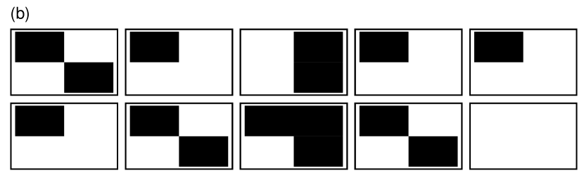
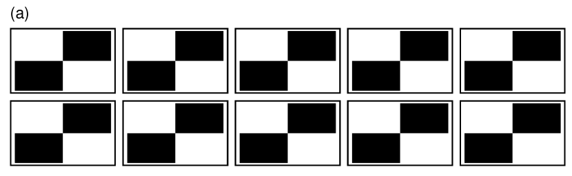
Figure 1: Ten 4-pixel images simulated from a degenerate model (a) compared to ten 4-pixel images simulated from a non-degenerate model (b). The degenerate model places almost all probability on one outcome, causing the image to be generated repeatedly, whereas the non-degenerate model shows more realistic variation.

In addition to such degeneracy, we find that RBMs can easily exhibit types of instability, related to how sensitive the model probabilities can be to small difference in data outcomes. In practice, this may be seen when a single pixel change in an image results in a wildly different classification in an image classification problem. Occurrences of such behavior have recently been documented in RBMs (Li 2014), as well as other deep architectures (Szegedy et al. 2013; Nguyen, Yosinski, and Clune 2014). We describe (related) potential issues of model instability, degeneracy and uninterpretability for the RBM class (which are related properties) and examine the presence of these in Section 3 through simulations of small, manageable examples.

Separate from the exploration of model properties, we also investigate the quality of estimation possible in fitting these models and examine an estimation procedure that allows for uncertainty quantification rather than point estimates alone. The fitting of RBMs can be problematic for two reasons, the first being computational and the second concerning flexibility. As the size of these models grows, both maximum likelihood and Bayesian methods of fitting quickly become intractable. The literature often suggests Markov chain Monte Carlo (MCMC) tools for approximate maximization of likelihoods to fit these models (e.g., Gibbs sampling to exploit conditional structure in hidden and visible variables), but little is said about the attributes of realized estimates (Hinton 2010; Hinton, Osindero, and Teh 2006), including the absence of interval estimates.

Furthermore, these MCMC algorithms involve updating potentially many latent variables (hiddens) which can critically influence convergence in MCMC-based likelihood methods. Applying basic statistical principles in fitting RBM models of tractable size, we compare three fully Bayesian techniques involving MCMC, which are computationally more accessible than direct maximum likelihood and also aim to avoid parts of a RBM parameter space that yield unattractive models. As might be expected, with greater computational complexity comes an increase in fitting accuracy, but at the cost of practical feasibility.

As a factor compounding the computational challenges, issues in model fitting traceable to model flexibility are potentially more concerning. For a RBM model with enough hidden variables, any distribution for the visibles can be approximated arbitrarily well (Le Roux and Bengio 2008; Montufar and Ay 2011; and Montúfar, Rauh, and Ay 2011). However, for binary data, the empirical distribution of an observed training set of visible variables provides a highest likelihood benchmark, before any parametric model class is even introduced and applied to obtain a refinement of model fit. As a consequence, we find that any fully principled fitting method based on the likelihood for a RBM with enough hidden variables will seek to reproduce the (discrete) empirical distribution of a training set. This aspect can be undesirable, and perhaps even unexpected compared to most modeling scenarios, in that no “smoothed distribution” may result when fitting a RBM model of sufficient size with a rigorous likelihood-based method. We are therefore led to be skeptical that models that involve these structures (like deep Boltzmann machines) can achieve useful prediction or inference in a principled way without intentionally limiting the flexibility of the fitted model.

Notions of weight-decay (penalization) and sparsity (regularization) have been suggested in the RBM literature as practical remedies for both over-fitting and poor mixing in the Markov chain during fitting (Hinton 2010; Tieleman 2008; Cho, Ilin, and Raiko 2012). Both $L_{1}$ and $L_{2}$ type penalties are mentioned to achieve weight-decay, though the benefits of these particular forms are unknown in different situations. The degree to which regularization and penalization are used by practitioners is not clear because these concepts are not (by default) a part of the standard overall model-specification-and-fitting methodology (Hinton 2002; Carreira-Perpinan and Hinton 2005). In this paper, we attempt to address the concerns with overfitting and poor mixing in an alternative (and perhaps more transparent) manner, via specification of a Bayesian prior in Section 4.1.

This paper is structured as follows. Section 2 formally defines the RBM including the joint distribution of hidden and visible variables and explains the model’s connection to deep learning. Additionally, measures of model impropriety and methods of quantifying/detecting it are defined. Section 3 details our explorations into the model behavior and potential propriety issues with the RBM class. This work aligns with the call to action by Google scientists in Sculley et al. (2018) to employ small toy examples to advance empirical understanding of deep learning models and strive for a “higher level of empirical rigor in the field.” We examine three Bayesian fitting techniques intended to avoid model impropriety issues raised in Section 4 and conclude with a discussion in Section 5. Supplementary online material provides proofs for results on RBM parameterizations and data codings described in Section 3.1.2.

While applications of the RBM have been claimed to produce some successes in classification problems, it is unclear if the model class allows one to go beyond fitting to other statistical matters of importance in using the models, such as quantification of the uncertainty of estimation and the formulation of predictive distributions. These are closely tied to the probability properties of the RBM model for explaining data generation and our exposition intends to contribute to a better understanding in this direction.

2 Background

2.1 Restricted Boltzmann machines

A restricted Boltzmann machine (RBM) is an undirected graphical model specified for discrete or continuous random variables, binary variables being most commonly considered. In this paper, we consider the binary case for concreteness. A RBM architecture has two layers, hidden ($\mathcal{H}$) and visible ($\mathcal{V}$), with no dependency connections within a layer. An example of this structure is in Figure 2 with the hidden nodes indicated by gray circles and the visible nodes indicated by white circles.

Figure 2: An example restricted Boltzmann machine (RBM), consisting of two layers, one hidden ($\mathcal{H}$) and one visible ($\mathcal{V}$), with no connections within a layer. Hidden nodes are indicated by gray filled circles and the visible nodes indicated by unfilled circles.

A common use for RBMs is to create features for use in classification. For example, binary images can be classified through a process that treats the pixel values as the visible variables $v_{i}$ in a RBM model (Hinton, Osindero, and Teh 2006).

2.1.1 Joint distribution

Let $\bm{x}=(h_{1},\dots,h_{n_{\scriptscriptstyle H}},v_{1},\dots,v_{n_{\scriptscriptstyle V}})$ represent the states of the visible and hidden nodes in a RBM for some integers ${n_{\scriptscriptstyle V}},{n_{\scriptscriptstyle H}}\geq 1$. Each single binary random variable, visible or hidden, will take its values in a common coding set $\mathcal{C}$, where we allow (one of) two possibilities for the coding set, $\mathcal{C}=\{0,1\}$ or $\mathcal{C}=\{-1,1\}$, with “$1$” always indicating the “high” value of the variable. While $\mathcal{C}=\{0,1\}$ may be a natural starting point, we argue in Section 3 that the coding $\mathcal{C}=\{-1,1\}$ induces more interpretable model properties for the RBM. A standard parametric form for probabilities corresponding to a potential vector of states, $X=(H_{1},\dots,H_{n_{\scriptscriptstyle H}},V_{1},\dots,V_{n_{\scriptscriptstyle V}})$, for the nodes is

$$f_{\bm{\theta}}(\bm{x})\equiv P_{\bm{\theta}}(\bm{X}=\bm{x})=\frac{\exp\left(\sum\limits_{i=1}^{n_{\scriptscriptstyle V}}\sum\limits_{j=1}^{n_{\scriptscriptstyle H}}\theta_{ij}v_{i}h_{j}+\sum\limits_{i=1}^{n_{\scriptscriptstyle V}}\theta_{v_{i}}v_{i}+\sum\limits_{j=1}^{n_{\scriptscriptstyle H}}\theta_{h_{j}}h_{j}\right)}{\gamma(\bm{\theta})},\quad\bm{x}\in\mathcal{C}^{{n_{\scriptscriptstyle H}}+{n_{\scriptscriptstyle V}}}$$ (1)

where $\bm{\theta}\equiv(\theta_{11},\dots,\theta_{1{n_{\scriptscriptstyle H}}},\dots,\theta_{{n_{\scriptscriptstyle V}}1},\dots,\theta_{{n_{\scriptscriptstyle V}}{n_{\scriptscriptstyle H}}},\theta_{v_{1}},\dots,\theta_{v_{n_{\scriptscriptstyle V}}},\theta_{h_{1}},\dots,\theta_{h_{n_{\scriptscriptstyle H}}})\in\mathbb{R}^{{n_{\scriptscriptstyle V}}+{n_{\scriptscriptstyle H}}+{n_{\scriptscriptstyle V}}*{n_{\scriptscriptstyle H}}}$ denotes the vector of model parameters and the denominator

$$\gamma(\bm{\theta})=\sum_{\bm{x}\in\mathcal{C}^{{n_{\scriptscriptstyle H}}+{n_{\scriptscriptstyle V}}}}\exp\left(\sum_{i=1}^{n_{\scriptscriptstyle V}}\sum_{j=1}^{n_{\scriptscriptstyle H}}\theta_{ij}v_{i}h_{j}+\sum_{i=1}^{n_{\scriptscriptstyle V}}\theta_{v_{i}}v_{i}+\sum_{j=1}^{n_{\scriptscriptstyle H}}\theta_{h_{j}}h_{j}\right)$$

is the normalizing function that ensures the probabilities (1) sum to one. For $\bm{x}=(h_{1},\dots,h_{n_{\scriptscriptstyle H}},v_{1},\dots,v_{n_{\scriptscriptstyle H}})\in\mathcal{C}^{{n_{\scriptscriptstyle V}}+{n_{\scriptscriptstyle H}}}$ and

$$\bm{t}(\bm{x}) =(h_{1},\dots,h_{n_{\scriptscriptstyle H}},v_{1},\dots,v_{n_{\scriptscriptstyle V}},v_{1}h_{1},\dots,v_{n_{\scriptscriptstyle V}}h_{n_{\scriptscriptstyle H}})\in\mathcal{C}^{{n_{\scriptscriptstyle H}}+{n_{\scriptscriptstyle V}}+{n_{\scriptscriptstyle H}}*{n_{\scriptscriptstyle V}}},$$ (2)

let $\mathcal{T}=\{\bm{t}(\bm{x}):\bm{x}\in\mathcal{C}^{{n_{\scriptscriptstyle V}}+{n_{\scriptscriptstyle H}}}\}\subset\mathbb{R}^{{n_{\scriptscriptstyle V}}+{n_{\scriptscriptstyle H}}+{n_{\scriptscriptstyle V}}*{n_{\scriptscriptstyle H}}}$ be the set of possible values for the vector of variables needed to compute probabilities (1) in the model, and write $Q_{\bm{\theta}}(\bm{x})=\sum\limits_{i=1}^{n_{\scriptscriptstyle H}}\sum\limits_{j=1}^{n_{\scriptscriptstyle V}}\theta_{ij}h_{i}v_{j}+\sum\limits_{i=1}^{n_{\scriptscriptstyle H}}\theta_{hi}h_{i}+\sum\limits_{j=1}^{n_{\scriptscriptstyle V}}\theta_{vj}v_{j}$ for the “neg-potential” function. The RBM model is parameterized by $\bm{\theta}$ containing two types of parameters, main effects and interaction effects. The main effects parameters ($\{\theta_{v_{i}},\theta_{h_{j}}\}_{\begin{subarray}{c}i=1,\dots,{n_{\scriptscriptstyle V}},\\ j=1,\dots,{n_{\scriptscriptstyle H}}\end{subarray}}$) weight the values of the visible $v_{i}$ and hidden $h_{j}$ nodes in probabilities (1) and the interaction effect parameters ($\theta_{ij}$) weight the values of the connections $v_{i}h_{j}$, or dependencies, between hidden and visible layers.

Due to the potential size of the model, the normalizing constant $\gamma(\bm{\theta})$ can be practically impossible to calculate, making simple estimation of the model parameter vector problematic. In model fitting, a kind of Gibbs sampling can be tried due to the conditional architecture of the RBM (i.e. visibles given hiddens or vice verse). Specifically, the conditional independence of nodes in each layer (given those nodes in the other layer) allows for stepwise simulation of both hidden layers and model parameters (e.g., see the contrastive divergence of Hinton (2002) or Bayes methods in Section 4).

2.1.2 Connection to Deep Learning

RBMs have risen to prominence in recent years due to their connection to deep learning (see Hinton, Osindero, and Teh 2006; Salakhutdinov and Hinton 2012; Srivastava, Salakhutdinov, and Hinton 2013 for examples). By stacking multiple layers of RBMs in a deep architecture, proponents of the methodology claim to produce the ability to learn “internal representations that become increasingly complex, which is considered to be a promising way of solving object and speech recognition problems” (Salakhutdinov and Hinton 2009, 450). The stacking is achieved by treating a hidden layer of one RBM as the visible layer in a second RBM, and so on, until the desired multi-layer architecture is created.

2.2 Degeneracy, instability, and uninterpretability

The highly flexible nature of a RBM (having as it does ${n_{\scriptscriptstyle H}}+{n_{\scriptscriptstyle V}}+{n_{\scriptscriptstyle H}}*{n_{\scriptscriptstyle V}}$ parameters) creates at least three kinds of potential issues of model impropriety that we will call degeneracy, instability, and uninterpretability. In this section we define these, consider how to quantify them in a RBM, and point out relationships among them.

2.2.1 Near-degeneracy

In Random Graph Model theory, model degeneracy means there is a disproportionate amount of probability placed on only a few elements of the sample space, $\mathcal{X}$, by the model (Handcock 2003). For random graph models, $\mathcal{X}$ denotes all possible graphs that can be constructed from a set of nodes and an exponentially parameterized random graph model has a distribution with a probability mass function of the form

$$f_{\bm{\theta}}(\bm{x})=\frac{\exp\left(\bm{\theta}^{T}\bm{t}(\bm{x})\right)}{\gamma(\bm{\theta})},\bm{x}\in\mathcal{X},$$

where $\bm{\theta}\in\Theta\subset\mathbb{R}^{q}$ is the model parameter, and $\bm{t}:\mathcal{X}\rightarrow\mathbb{R}^{q}$ is a vector of statistics based on the adjacency matrix of a graph. Here, as earlier for RBMs, $\gamma(\bm{\theta})=\sum_{\bm{x}\in\mathcal{X}}\exp\left(\bm{\theta}^{T}\bm{t}(\bm{x})\right)$ is the normalizing function. Let $C$ denote the convex hull of the potential outcomes of sufficient statistics, $\{\bm{t}(\bm{x}):\bm{x}\in\mathcal{X}\}$, under the model above. Handcock (2003) classifies an exponentially parameterized random graph model at $\bm{\theta}$ as near-degenerate if the mean value of the vector of sufficient statistics under $\bm{\theta}$, $\bm{\mu}(\bm{\theta})=\text{E}_{\bm{\theta}}\bm{t}(\bm{X})$, is close to the boundary of $C$. Intuitively, if a model is near-degenerate in the sense that only a small number of elements of the sample space $\mathcal{X}$ have positive probability, the expected value $\text{E}_{\bm{\theta}}\bm{t}(\bm{X})$ is an average of that same small number of values of $t(\bm{x})$ (defining the boundary of the hull $C$) and can be expected to not be pulled deep into the interior of $C$.

A RBM model can be thought to exhibit an analogous form of near-degeneracy when there is a disproportionate amount of probability placed on a small number of elements in the sample space of visibles and hiddens, $\mathcal{C}^{{n_{\scriptscriptstyle V}}+{n_{\scriptscriptstyle H}}}$. Using the idea of Handcock (2003), when the random vector $\bm{t}(\bm{x})=(v_{1},\dots,v_{n_{\scriptscriptstyle V}},h_{1},\dots,h_{n_{\scriptscriptstyle H}},v_{1}h_{1},\dots,v_{V}h_{n_{\scriptscriptstyle H}})\in\mathcal{T}\equiv\{\bm{t}(\bm{x}):\bm{x}\in\mathcal{C}^{{n_{\scriptscriptstyle H}}+{n_{\scriptscriptstyle V}}}\}$ from (2), appearing in the neg-potential function $Q_{\bm{\theta}}(\cdot)$, has a mean vector $\bm{\mu}(\bm{\theta})\in\mathbb{R}^{{n_{\scriptscriptstyle V}}+{n_{\scriptscriptstyle H}}+{n_{\scriptscriptstyle V}}*{n_{\scriptscriptstyle H}}}$ close to the boundary of the convex hull of $\mathcal{T}$, and the RBM model can be said to exhibit near-degeneracy at $\bm{\theta}\in\mathbb{R}^{{n_{\scriptscriptstyle V}}+{n_{\scriptscriptstyle H}}+{n_{\scriptscriptstyle H}}*{n_{\scriptscriptstyle V}}}$. Here the mean of $\bm{t}(\bm{x})$ is

$$\bm{\mu}(\bm{\theta})=\text{E}_{\bm{\theta}}\bm{t}(\bm{X}) =\sum\limits_{x\in\mathcal{C}^{{n_{\scriptscriptstyle V}}+{n_{\scriptscriptstyle H}}}}\left\{\bm{t}(\bm{x})f_{\bm{\theta}}(\bm{x})\right\}$$

$$=\sum\limits_{x\in\mathcal{C}^{{n_{\scriptscriptstyle V}}+{n_{\scriptscriptstyle H}}}}\left\{\bm{t}(\bm{x})\dfrac{\exp\left(\sum\limits_{i=1}^{n_{\scriptscriptstyle V}}\sum\limits_{j=1}^{n_{\scriptscriptstyle H}}\theta_{ij}v_{i}h_{j}+\sum\limits_{i=1}^{n_{\scriptscriptstyle V}}\theta_{v_{i}}v_{i}+\sum\limits_{j=1}^{n_{\scriptscriptstyle H}}\theta_{h_{j}}h_{j}\right)}{\sum\limits_{\bm{x}\in\mathcal{C}^{{n_{\scriptscriptstyle H}}+{n_{\scriptscriptstyle V}}}}\exp\left(\sum\limits_{i=1}^{n_{\scriptscriptstyle V}}\sum\limits_{j=1}^{n_{\scriptscriptstyle H}}\theta_{ij}v_{i}h_{j}+\sum\limits_{i=1}^{n_{\scriptscriptstyle V}}\theta_{v_{i}}v_{i}+\sum\limits_{j=1}^{n_{\scriptscriptstyle H}}\theta_{h_{j}}h_{j}\right)}\right\}.$$

2.2.2 Instability

Considering exponential families of distributions, Schweinberger (2011) introduced a concept of model deficiency related to instability. Instability can be roughly thought of as excessive sensitivity in the model, where small changes in the components of potential data outcomes, $\bm{x}$, may lead to substantial changes in the probability mass function $f_{\bm{\theta}}(\bm{x})$. Furthermore, model instability can be viewed on a spectrum of potential sensitivity in probability structure, with model degeneracy included as a extreme or limiting case of instability. To quantify “instability” more rigorously (particularly beyond the definition given by Schweinberger (2011)) it is useful to consider how RBM models might be expanded to incorporate more and more visibles. When increasing the size of RBM models, it becomes necessary to grow the number of model parameters (and in this process one may also arbitrarily expand the number of hidden variables used). To this end, let $\bm{\theta}_{{n_{\scriptscriptstyle V}}}\equiv(\theta_{v_{1}},\dots,\theta_{v_{n_{\scriptscriptstyle V}}},\theta_{h_{1}},\dots,\theta_{h_{n_{\scriptscriptstyle H}}},\theta_{11},\dots,\theta_{{n_{\scriptscriptstyle V}}{n_{\scriptscriptstyle H}}}),{n_{\scriptscriptstyle V}}\geq 1$, denote an element of a sequence of RBM parameters indexed by the number ${n_{\scriptscriptstyle V}}$ of visibles $(V_{1},\dots,V_{n_{\scriptscriptstyle V}})$ and define a log-ratio of extremal probabilities (LREP) of the RBM model at $\bm{\theta}_{{n_{\scriptscriptstyle V}}}$ as

$$\frac{1}{{n_{\scriptscriptstyle V}}}\log\left[\frac{\max\limits_{(v_{1},\dots,v_{n_{\scriptscriptstyle V}})\in\mathcal{C}^{n_{\scriptscriptstyle V}}}P_{\bm{\theta}_{n_{\scriptscriptstyle V}}}(v_{1},\dots,v_{n_{\scriptscriptstyle V}})}{\min\limits_{(v_{1},\dots,v_{n_{\scriptscriptstyle V}})\in\mathcal{C}^{n_{\scriptscriptstyle V}}}P_{\bm{\theta}_{n_{\scriptscriptstyle V}}}(v_{1},\dots,v_{n_{\scriptscriptstyle V}})}\right]\equiv\frac{1}{{n_{\scriptscriptstyle V}}}\text{LREP}(\bm{\theta}_{n_{\scriptscriptstyle V}})$$ (3)

where $P_{\bm{\theta}_{n_{\scriptscriptstyle V}}}(v_{1},\dots,v_{n_{\scriptscriptstyle V}})\propto\sum_{(h_{1},\dots,h_{n_{\scriptscriptstyle H}})\in\mathcal{C}^{n_{\scriptscriptstyle H}}}\exp\left(\sum_{i=1}^{n_{\scriptscriptstyle V}}\theta_{v_{i}}v_{i}+\sum_{j=1}^{n_{\scriptscriptstyle H}}\theta_{h_{j}}h_{j}+\sum_{i=1}^{n_{\scriptscriptstyle V}}\sum_{j=1}^{n_{\scriptscriptstyle H}}\theta_{ij}v_{i}h_{j}\right)$ is the RBM probability of observing outcome $(v_{1},\dots,v_{n_{\scriptscriptstyle V}})$ for the visible variables $(V_{1},\dots,V_{n_{\scriptscriptstyle V}})$ under parameter vector $\bm{\theta}_{n_{\scriptscriptstyle V}}$, after marginalization of hidden variables.

In formulating a RBM model for a potentially large number of visibles (i.e., as ${n_{\scriptscriptstyle V}}\rightarrow\infty$), we will say that the ratio (3) needs to stay bounded for a sequence of RBM models to be stable. That is, we make the following convention.

Definition 2.1 (S-unstable RBM).

Let $\bm{\theta}_{n_{\scriptscriptstyle V}}\in\mathbb{R}^{{n_{\scriptscriptstyle V}}+{n_{\scriptscriptstyle H}}+{n_{\scriptscriptstyle H}}*{n_{\scriptscriptstyle V}}},{n_{\scriptscriptstyle V}}\geq 1$, be an element of a sequence of RBM parameters where the number of hiddens, ${n_{\scriptscriptstyle H}}\equiv{n_{\scriptscriptstyle H}}({n_{\scriptscriptstyle V}})\geq 1$, can be an arbitrary function of the number ${n_{\scriptscriptstyle V}}$ of visibles. A RBM model formulation is Schweinberger-unstable or S-unstable if

$$\lim\limits_{{n_{\scriptscriptstyle V}}\rightarrow\infty}\frac{1}{{n_{\scriptscriptstyle V}}}\text{LREP}(\bm{\theta}_{n_{\scriptscriptstyle V}})=\infty.$$

In other words, a RBM model sequence is unstable if, given any $c>0$, there exists an integer $n_{c}>0$ so that $\frac{1}{{n_{\scriptscriptstyle V}}}\text{LREP}(\bm{\theta}_{n_{\scriptscriptstyle V}})>c$ for all ${n_{\scriptscriptstyle V}}\geq n_{c}$. This definition of S-unstable is a generalization or re-interpretation of the “unstable” concept of Schweinberger (2011) in that here RBM models for visibles $(v_{1},\dots,v_{n_{\scriptscriptstyle V}})$ do not form an exponential family and the dimensionality of $\bm{\theta}_{n_{\scriptscriptstyle V}}$ is not fixed, but rather grows with ${n_{\scriptscriptstyle V}}$.

S-unstable RBM model sequences are undesirable for several reasons. One is that, as mentioned above, small changes in data can lead to overly-sensitive changes in probability under the data model. Consider, for example,

$$\Delta(\bm{\theta}_{n_{\scriptscriptstyle V}})\equiv\max\left\{\log\frac{P_{\bm{\theta}_{n_{\scriptscriptstyle V}}}(\bm{v})}{P_{\bm{\theta}_{n_{\scriptscriptstyle V}}}(\bm{v}^{*})}:\bm{v}\text{ }\&\text{ }\bm{v}^{*}\in\mathcal{C}^{n_{\scriptscriptstyle V}}\text{ differ in exactly one component}\right\},$$

denoting the biggest log-probability ratio for a one-component change in data outcomes (visibles) at a RBM parameter $\bm{\theta}_{n_{\scriptscriptstyle V}}$. We then have the following result.

Proposition 2.2.

Let $c>0$ and let $\text{LREP}(\bm{\theta}_{n_{\scriptscriptstyle V}})$ be as in (3) for an integer ${n_{\scriptscriptstyle V}}\geq 1$. If $\frac{1}{{n_{\scriptscriptstyle V}}}\text{LREP}(\bm{\theta}_{n_{\scriptscriptstyle V}})>c$, then $\Delta(\bm{\theta}_{n_{\scriptscriptstyle V}})>c$.

In other words, if the probability ratio (3) is too large, then a RBM model sequence will exhibit large probability shifts for very small changes in data configurations (i.e., will exhibit instability). Such instability can be a concern in a model for reasons similar to those related to degeneracy: as outcomes vary over the sample space, the geography of probabilities is extremely rugged, with deep pits following sharp mountains. Recall the applied example of RBM models as a means to classify images. For data as pixels in an image, the instability result in Proposition 2.2 manifests itself as a one pixel change in an image (one component of the visible vector) resulting in a large shift in the probability, which in turn could result in a vastly different classification of the image. Examples of this kind of behavior have been presented in Szegedy et al. (2013) for deep learning models, in which a one pixel change in a test image results in a wildly different classification.

Additionally, S-unstable RBM model sequences may be formally connected to the near-degeneracy of Section 2.2.1 (in which model sequences place all probability on a small portion of their sample spaces). To see this, define an arbitrary modal set of possible outcomes (i.e. set of highest probability outcomes) in RBM models with parameters $\bm{\theta}_{n_{\scriptscriptstyle V}},{n_{\scriptscriptstyle V}}\geq 1$ as

$$M_{\epsilon,\bm{\theta}_{n_{\scriptscriptstyle V}}}\equiv\left\{\bm{v}\in\mathcal{C}^{n_{\scriptscriptstyle V}}:\log P_{\bm{\theta}_{n_{\scriptscriptstyle V}}}(\bm{v})>(1-\epsilon)\max\log\limits_{\bm{v}^{*}}P_{\bm{\theta}_{n_{\scriptscriptstyle V}}}(\bm{v}^{*})+\epsilon\min\log\limits_{\bm{v}^{*}}P_{\bm{\theta}_{n_{\scriptscriptstyle V}}}(\bm{v}^{*})\right\}$$

for a given $0<\epsilon<1$. Then S-unstable model sequences are guaranteed to be degenerate, as the following result shows.

Proposition 2.3.

For an S-unstable RBM model sequence and any $0<\epsilon<1$,

$$P_{\bm{\theta}_{n_{\scriptscriptstyle V}}}\left((v_{1},\dots,v_{n_{\scriptscriptstyle V}})\in M_{\epsilon,\bm{\theta}_{n_{\scriptscriptstyle V}}}\right)\rightarrow 1\text{ as }{n_{\scriptscriptstyle V}}\rightarrow\infty.$$

In other words, S-unstable RBM model sequences are guaranteed to stack up all probability on a specific set of outcomes for visibles, which could potentially be arbitrarily narrow. Proofs of Propositions 2.2 and 2.3 follow from more general results in Kaplan, Nordman, and Vardeman (2017). These findings also have counterparts in results in Schweinberger (2011), but unlike results there, are not limited in consideration to exponential family forms with a fixed number of parameters.

2.2.3 Uninterpretability

For spatial Markov models, Kaiser (2007) defines a measure of model impropriety he calls uninterpretability, which is characterized by dependence parameters in a model being so extreme that marginal mean-structures fail to hold as anticipated by consideration of a model statement. We adapt this notion to RBM models. Note that in a RBM, the parameters $\theta_{v_{1}},\dots,\theta_{v_{n_{\scriptscriptstyle V}}}$ and $\theta_{h_{1}},\dots,\theta_{h_{n_{\scriptscriptstyle H}}}$ are naturally associated with main effects of visible and hidden variables and can be interpreted as (logit functions of) means for variables $V_{1},\dots,V_{n_{\scriptscriptstyle V}},H_{1},\dots,H_{n_{\scriptscriptstyle H}}$ in a model with no interaction parameters, $\theta_{ij}=0,i=1,\dots,{n_{\scriptscriptstyle V}},j=1,\dots,{n_{\scriptscriptstyle H}}$. That is, with no interaction parameters, we have from (1) that

$$P_{\theta}(V_{i}=1)\propto e^{\theta_{v_{i}}}\quad\text{ and }\quad P_{\theta}(H_{j}=1)\propto e^{\theta_{h_{j}}},\quad i=1,\ldots,{n_{\scriptscriptstyle V}},j=1,\ldots,{n_{\scriptscriptstyle H}}$$

so that, for example, $\text{logit}(P_{\theta}(V_{i}=1))=\theta_{v_{i}}$ (or $2\theta_{v_{i}}$) under the coding $\mathcal{C}=\{0,1\}$ (or $\{-1,1\}$). Hence, these main effect parameters have a clear interpretation under an independence model (one with $\theta_{ij}=0$) but this interpretation can break down as interaction parameters increase in magnitude relative to the size of the main effects. In such cases, the main effect parameters $\theta_{v_{1}}$ and $\theta_{h_{j}}$ are no longer interpretable in the models (statements of marginal means) and the dependence parameters are so large as to dominate the entire model probability structure (also destroying simple interpretation of dependence parameters $\theta_{ij}$, $j=1,\ldots,{n_{\scriptscriptstyle H}}$ as local conditional modifications of an overall marginal mean structure $\theta_{v_{i}}$, as appearing for example in the (logit) conditional probability $\mathrm{logitP_{\theta}(V_{i}=1|H_{1},\ldots,H_{{n_{\scriptscriptstyle H}}})}=\theta_{v_{i}}+\sum_{j=1}^{{n_{\scriptscriptstyle H}}}\theta_{ij}H_{j}$). Whether or not parameter interpretation is itself a goal in a given application of RBM models, this concept of interpretation can provide an additional device for examining other aspects of model propriety related to instability and degeneracy. As explained by Kaiser (2007), models with interpretable dependence parameters typically correspond to non-degenerate models, while degradation in interpretability is often associated with model drift into degeneracy. To assess which parameter values $\bm{\theta}$ may cause difficulties in interpretation, we use the difference $\text{E}\left[\bm{X}|\bm{\theta}\right]-\text{E}\left[\bm{X}|\bm{\theta}^{*}\right]$ between two model expectations: E$\left[\bm{X}|\bm{\theta}\right]$ at $\bm{\theta}$ and expectations E$\left[\bm{X}|\bm{\theta}^{*}\right]$ where $\bm{\theta}^{*}$ matches $\bm{\theta}$ for all main effects but otherwise has $\theta_{ij}=0$ for $i=1,\dots,{n_{\scriptscriptstyle V}},j=1,\dots,{n_{\scriptscriptstyle H}}$. (Hence, $\bm{\theta}^{*}$ and $\bm{\theta}$ have the same main effects but $\bm{\theta}^{*}$ has $0$ dependence parameters.) Uninterpretability is then avoided at a parametric specification $\bm{\theta}$ if the model expected value at $\bm{\theta}$ is not very different from the corresponding model expectation under independence. Using this, it is possible to investigate what parametric conditions lead to uninterpretability in a model versus those that guarantee interpretable models. If $\text{E}\left[\bm{X}|\bm{\theta}\right]-\text{E}\left[\bm{X}|\bm{\theta}^{*}\right]$ is large, then the RBM model with parameter vector $\bm{\theta}$ is said to be uninterpetable. The quantities to compare in the RBM case are

$$\text{E}\left[\bm{X}|\bm{\theta}\right]=\sum\limits_{\bm{x}\in\mathcal{C}^{{n_{\scriptscriptstyle V}}+{n_{\scriptscriptstyle H}}}}\bm{x}f_{\bm{\theta}}(\bm{x})=\sum\limits_{\bm{x}\in\mathcal{C}^{{n_{\scriptscriptstyle V}}+{n_{\scriptscriptstyle H}}}}\bm{x}\frac{\exp\left(\sum\limits_{i=1}^{n_{\scriptscriptstyle V}}\sum\limits_{j=1}^{n_{\scriptscriptstyle H}}\theta_{ij}v_{i}h_{j}+\sum\limits_{i=1}^{n_{\scriptscriptstyle V}}\theta_{v_{i}}v_{i}+\sum\limits_{j=1}^{n_{\scriptscriptstyle H}}\theta_{h_{j}}h_{j}\right)}{\sum\limits_{\bm{x}\in\mathcal{C}^{{n_{\scriptscriptstyle V}}+{n_{\scriptscriptstyle H}}}}\exp\left(\sum\limits_{i=1}^{n_{\scriptscriptstyle V}}\sum\limits_{j=1}^{n_{\scriptscriptstyle H}}\theta_{ij}v_{i}h_{j}+\sum\limits_{i=1}^{n_{\scriptscriptstyle V}}\theta_{v_{i}}v_{i}+\sum\limits_{j=1}^{n_{\scriptscriptstyle H}}\theta_{h_{j}}h_{j}\right)}$$

and

$$\text{E}\left[\bm{X}|\bm{\theta}^{*}\right] =\sum\limits_{\bm{x}\in\mathcal{C}^{{n_{\scriptscriptstyle V}}+{n_{\scriptscriptstyle H}}}}\bm{x}\frac{\exp\left(\sum\limits_{i=1}^{n_{\scriptscriptstyle V}}\theta_{v_{i}}v_{i}+\sum\limits_{j=1}^{n_{\scriptscriptstyle H}}\theta_{h_{j}}h_{j}\right)}{\sum\limits_{\bm{x}\in\mathcal{C}^{{n_{\scriptscriptstyle V}}+{n_{\scriptscriptstyle H}}}}\exp\left(\sum\limits_{i=1}^{n_{\scriptscriptstyle V}}\theta_{v_{i}}v_{i}+\sum\limits_{j=1}^{n_{\scriptscriptstyle H}}\theta_{h_{j}}h_{j}\right)}$$

3 Explorations of model properties through simulation

We next explore and numerically explain the relationship between values of $\bm{\theta}$ and the three notions of model impropriety (near-degeneracy, instability, and uninterpretability), for RBM models of varying sizes.

3.1 Tiny example

To illustrate the ideas of model near-degeneracy, instability, and uninterpretability in a RBM, we consider first the smallest possible (toy) example that consists of one visible node $v_{1}$ and one hidden node $h_{1}$ that are both binary. A schematic of this model can be found in Figure 3. Because it seems most common, we shall begin by employing $0/1$ encoding of binary variables (both $h_{1}$ and $v_{1}$ taking values in $\mathcal{C}=\{0,1\}$). (Eventually we shall argue in Section 3.1.2 that $-1/1$ coding has advantages.)

Figure 3: A small example restricted Boltzmann machine (RBM), with two nodes, one hidden and one visible.

3.1.1 Impropriety three ways

For this small model, we are able to investigate the symptoms of model impropriety, beginning with near-degeneracy. To this end, recall from Section 2.2.1 that one characterization requires consideration of the convex hull of possible values of statistics $\bm{t}(\bm{x})$,

$$\mathcal{T}=\{\bm{t}(\bm{x}):\bm{x}=(v_{1},h_{1})\in\{0,1\}^{2}\}\equiv\{(v_{1},h_{1},v_{1}h_{1}):v_{1},h_{1}\in\{0,1\}\}$$

appearing in the RBM probabilities for this model. As this set is in three dimensions, we are able to explicitly illustrate the shape of boundary of the convex hull of $\mathcal{T}$ and explore the behavior of the mean vector $\bm{\mu}(\bm{\theta})=\text{E}_{\bm{\theta}}\bm{t}(\bm{x})$ as a function of the parameter vector $\bm{\theta}$. Figure 4 shows the convex hull of our “statistic space,” $\mathcal{T}\subset\{0,1\}^{3}$, for this toy problem from two perspectives (enclosed by the unit cube $[0,1]^{3}$, the convex hull of $\{0,1\}^{3}$). In this small model, note that the convex hull of $\mathcal{T}$ does not fill the unrestricted hull of $\{0,1\}^{3}$ because of the relationship between the elements of $\mathcal{T}=\{(v_{1},h_{1},v_{1}h_{1}:v_{1},h_{1}\in\{0,1\}\}$ (i.e. $v_{1}h_{1}=1$ only if $v_{1}=h_{1}=1$).

Figure 4: Two perspectives of the convex hull of the “statistic space" in three dimensions for the toy RBM with one visible and one hidden node.

We can compute the mean vector for $\bm{t}(\bm{x})$ as a function of the model parameters as

$$\bm{\mu}(\bm{\theta})=\text{E}_{\bm{\theta}}\left[\bm{t}(\bm{X})\right]=\sum\limits_{\bm{x}=(v_{1},h_{1})\in\{0,1\}^{2}}\left\{t(x)\frac{\exp\left(\theta_{11}h_{1}v_{1}+\theta_{h1}h_{1}+\theta_{v1}v_{1}\right)}{\gamma(\bm{\theta})}\right\}=\left[\begin{matrix}\frac{\exp\left(\theta_{v_{1}}\right)+\exp\left(\theta_{11}+\theta_{v_{1}}+\theta_{h_{1}}\right)}{\gamma(\bm{\theta})}\\ \frac{\exp\left(\theta_{h_{1}}\right)+\exp\left(\theta_{11}+\theta_{v_{1}}+\theta_{h_{1}}\right)}{\gamma(\bm{\theta})}\\ \frac{\exp\left(\theta_{11}+\theta_{v_{1}}+\theta_{h_{1}}\right)}{\gamma(\bm{\theta})}\\ \end{matrix}\right]$$

where $\gamma(\bm{\theta})=\sum\limits_{h_{1}=0}^{1}\sum\limits_{v_{1}=0}^{1}\exp(\theta_{11}h_{1}v_{1}+\theta_{h_{1}}h_{1}+\theta_{v_{1}}v_{1})$. The three parametric coordinate functions of $\bm{\mu}(\bm{\theta})$ can be represented as in Figure 5. (Contour plots for three coordinate functions are shown in columns for various values of $\theta_{11}$, which can be interpreted here as an absolute log-odds ratio as the visible changes between $0$ and $1$.) In examining these, we see that as coordinates of $\bm{\theta}$ grow larger in magnitude, at least one mean function for the entries of $\bm{t}(\bm{x})$ approaches a value 0 or 1, forcing $\bm{\mu}(\bm{\theta})=\text{E}_{\bm{\theta}}\bm{t}(\bm{x})$ to be near to the boundary of the convex hull of $\mathcal{T}$, as a sign of model near-degeneracy. Thus, for a very small example we can see the relationship between values of $\bm{\theta}$ moving (sometimes only slightly) from zero and model degeneracy.

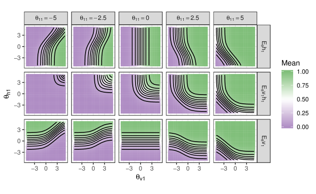
Figure 5: Contour plots for the three parametric mean functions of sufficient statistics for a RBM with one visible and one hidden node.

Secondly, we can look at $\text{LREP}(\bm{\theta})$ from (3) for this tiny model in order to consider model instability as a function of RBM parameters. Recall that large values of $\text{LREP}(\bm{\theta})$ are associated with an extreme sensitivity of the model probabilities $f_{\bm{\theta}}(\bm{x})$ to small changes in $\bm{x}$ (see Proposition 2.2). The quantity $\text{LREP}(\bm{\theta})$ for this small RBM is

$$\text{LREP}(\bm{\theta}) =\log\left[\frac{\max\limits_{(v_{1},\dots,v_{n_{\scriptscriptstyle V}})\in\mathcal{C}^{n_{\scriptscriptstyle V}}}P_{\bm{\theta}_{n_{\scriptscriptstyle V}}}(v_{1},\dots,v_{n_{\scriptscriptstyle V}})}{\min\limits_{(v_{1},\dots,v_{n_{\scriptscriptstyle V}})\in\mathcal{C}^{n_{\scriptscriptstyle V}}}P_{\bm{\theta}_{n_{\scriptscriptstyle V}}}(v_{1},\dots,v_{n_{\scriptscriptstyle V}})}\right]=\log\left[\frac{\max\limits_{v_{1}\in\mathcal{C}}\sum\limits_{h_{1}\in\mathcal{C}}\exp\left\{\theta_{11}h_{1}v_{1}+\theta_{h_{1}}h_{1}+\theta_{v_{1}}v_{1}\right\}}{\min\limits_{v_{1}\in\mathcal{C}}\sum\limits_{h_{1}\in\mathcal{C}}\exp\left\{\theta_{11}h_{1}v_{1}+\theta_{h_{1}}h_{1}+\theta_{v_{1}}v_{1}\right\}}\right].$$

Figure 6 shows contour plots of $\text{LREP}(\bm{\theta})/{n_{\scriptscriptstyle V}}$ for various values of $\bm{\theta}$ in this model with ${n_{\scriptscriptstyle V}}=1$. We can see that this quantity is large for large magnitudes of $\bm{\theta}$, especially for large values of the dependence/interaction parameter $\theta_{11}$. This suggests instability as $|\bm{\theta}|$ becomes large, agreeing also with the concerns about near-degeneracy produced by consideration of $\bm{\mu}(\bm{\theta})$.

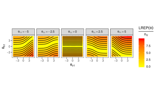
Figure 6: $\text{LREP}(\bm{\theta})/{n_{\scriptscriptstyle V}}$ for various values of $\bm{\theta}$ for the tiny example model. (Recall here ${n_{\scriptscriptstyle V}}$ is the number of visible nodes and here is $1$.) This quantity is large for large magnitudes of $\bm{\theta}$.

Finally to consider the effect of $\bm{\theta}$ on potential model uninterpretability, we can look at the difference between model expectations, E$\left[\bm{X}|\bm{\theta}\right]$, and expectations given independence, E$\left[\bm{X}|\bm{\theta}^{*}\right]$ for the tiny toy RBM model where $\bm{X}=(V_{1},H_{1},V_{1}H_{1})$. This difference is given by

$$\text{E}\left[\bm{X}|\bm{\theta}\right]-\text{E}\left[\bm{X}|\bm{\theta}^{*}\right] =\left[\begin{matrix}\frac{\exp\left(\theta_{11}+\theta_{v_{1}}+2\theta_{h_{1}}\right)-\exp\left(\theta_{v_{1}}+2\theta_{h_{1}}\right)}{\left(\exp\left(\theta_{v_{1}}\right)+\exp\left(\theta_{h_{1}}\right)+\exp\left(\theta_{11}+\theta_{v_{1}}+\theta_{h_{1}}\right)\right)\left(\exp\left(\theta_{v_{1}}\right)+\exp\left(\theta_{h_{1}}\right)+\exp\left(+\theta_{v_{1}}+\theta_{h_{1}}\right)\right)}\\ \frac{\exp\left(\theta_{11}+2\theta_{v_{1}}+\theta_{h_{1}}\right)-\exp\left(2\theta_{v_{1}}+\theta_{h_{1}}\right)}{\left(\exp\left(\theta_{v_{1}}\right)+\exp\left(\theta_{h_{1}}\right)+\exp\left(\theta_{11}+\theta_{v_{1}}+\theta_{h_{1}}\right)\right)\left(\exp\left(\theta_{v_{1}}\right)+\exp\left(\theta_{h_{1}}\right)+\exp\left(+\theta_{v_{1}}+\theta_{h_{1}}\right)\right)}\end{matrix}\right].$$

Again, we can inspect these coordinate functions of this vector difference to look for a relationship between parameter values and large values of $\text{E}[\bm{X}|\bm{\theta}]-\text{E}[\bm{X}|\bm{\theta}^{*}]$ as a signal of uninterpretability for the toy RBM.

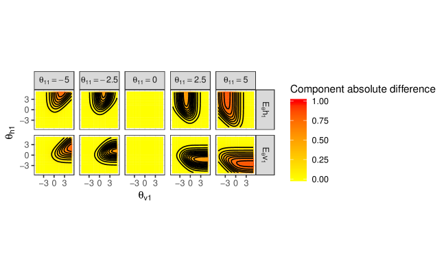
Figure 7: The absolute difference between coordinates of model expectations, E$\left[\bm{X}|\bm{\theta}\right]$, and expectations given independence, E$\left[\bm{X}|\bm{\theta}^{*}\right]$ for a RBM with one visible and one hidden node. As an indicator of uninterpretability, note that differences in expectations increase as the dependence parameter $\theta_{11}$ deviates from zero.

Figure 7 shows that the absolute difference between coordinates of the vector of model expectations, E$\left[\bm{X}|\bm{\theta}\right]$ and corresponding expectations E$\left[\bm{X}|\bm{\theta}^{*}\right]$ given independence grow for the toy RBM as the values of $\bm{\theta}$ are farther from zero, especially for large magnitudes of the dependence parameter $\theta_{11}$. This is a third indication that parameter vectors of large magnitude can readily lead to model impropriety in a RBM.

3.1.2 Data encoding

Multiple encodings of the binary variables are possible. For example, we could allow hiddens $(H_{1},\dots,H_{n_{\scriptscriptstyle H}})\in\{0,1\}^{n_{\scriptscriptstyle H}}$ and visibles $(V_{1},\dots,V_{n_{\scriptscriptstyle V}})\in\{0,1\}^{n_{\scriptscriptstyle V}}$, as in the previous sections or we could instead encode the state of the variables as $\{-1,1\}^{n_{\scriptscriptstyle H}}$ and $\{-1,1\}^{n_{\scriptscriptstyle V}}$. This will result in variables $\bm{t}(\bm{X})$ from (2) satisfying $\bm{t}(\bm{x})\in\{0,1\}^{{n_{\scriptscriptstyle H}}+{n_{\scriptscriptstyle V}}+{n_{\scriptscriptstyle H}}*{n_{\scriptscriptstyle V}}}$ or $\bm{t}(\bm{x})\in\{-1,1\}^{{n_{\scriptscriptstyle H}}+{n_{\scriptscriptstyle V}}+{n_{\scriptscriptstyle H}}*{n_{\scriptscriptstyle V}}}$ depending on how we encode “on” and “off” states in the nodes.

The $-1/1$ data encoding has the benefit of providing a guaranteed-to-be non-degenerate model at $\bm{\theta}=\bm{0}\in\mathbb{R}^{{n_{\scriptscriptstyle H}}+{n_{\scriptscriptstyle V}}+{n_{\scriptscriptstyle H}}*{n_{\scriptscriptstyle V}}}$, where the zero vector then serves as the natural center of the parameter space and induces the simplest possible model properties for the RBM (i.e., at $\bm{\theta}=\bm{0}$, all variables are independent uniformly distributed on $\{-1,1\}^{n_{\scriptscriptstyle V}}$). The proof of this and further exploration of the equivalence of the $\bm{\theta}$ parameterization of the RBM model class and parameterization by $\bm{\mu}(\bm{\theta})$ is in the on-line supplementary materials. Hence, while from some computing perspectives $0/1$ coding might seem most natural, the $-1/1$ coding is far more convenient and interpretable from the point of view of statistical modeling, where it makes parameters simply interpreted in terms of symmetrically defined main effects and interactions. Under the data encoding $-1/1$, the parameter space centered at 0 is also helpful for framing parameter configurations that are undesirably large (i.e., these are naturally parameters that have moved too far away from $\bm{0}$ where the RBM model is anchored to be trivially describable and completely problem-free). In light of all of these matters we will henceforth employ the $-1/1$ coding.

3.2 Exploring manageable examples

To explore the impact of RBM parameter vector $\bm{\theta}$ magnitude on near-degeneracy, instability, and uninterpretability, we consider models of small size. For ${n_{\scriptscriptstyle H}},{n_{\scriptscriptstyle V}}\in\{1,\dots,4\}$, we sample 100 values of $\bm{\theta}$ with various magnitudes (details to follow). For each set of parameters we then calculate metrics of model impropriety introduced in Section 2.2 based on $\bm{\mu}(\bm{\theta})$, $\text{LREP}(\bm{\theta})/{n_{\scriptscriptstyle V}}$, and the absolute coordinates of $\text{E}\left[\bm{X}|\bm{\theta}\right]-\text{E}\left[\bm{X}|\bm{\theta}^{*}\right]$. In the case of near-degeneracy, we classify each model as near-degenerate based on the distance of $\bm{\mu}(\bm{\theta})$ from the boundary of the convex hull of $\mathcal{T}$ and look at the fraction of models that are “near-degenerate,” meaning they are within a small distance $\epsilon>0$ of the boundary of the convex hull. We define “small” through a rough estimation of the volume of the hull for each model size. We pick $\epsilon_{0}=0.05$ for ${n_{\scriptscriptstyle H}}={n_{\scriptscriptstyle V}}=1$ and then, for every other ${n_{\scriptscriptstyle H}}$ and ${n_{\scriptscriptstyle V}}$, set $m={n_{\scriptscriptstyle H}}+{n_{\scriptscriptstyle V}}+{n_{\scriptscriptstyle V}}*{n_{\scriptscriptstyle H}}$ and pick $\epsilon$ so that $1-(1-2\epsilon_{0})^{3}=1-(1-2\epsilon)^{m}$. In this way, we roughly scale the volume of the “small distance” to the boundary of the convex hull to be equivalent across model dimensions.

In our numerical experiment, we split $\bm{\theta}=(\bm{\theta}_{main},\bm{\theta}_{interaction})$ into $\bm{\theta}_{main}$ and $\bm{\theta}_{interaction}$, in reference to which variables in the probability function the parameters correspond (whether they multiply a $v_{i}$ or a $h_{j}$ or they multiply a $v_{i}h_{j}$), and allow the two types of terms to have varying average magnitudes, $||\bm{\theta}_{main}||/({n_{\scriptscriptstyle H}}+{n_{\scriptscriptstyle V}})$ and $||\bm{\theta}_{interaction}||/({n_{\scriptscriptstyle H}}*{n_{\scriptscriptstyle V}})$. These average magnitudes vary on a $1$-dimensional grid between 0.001 and 3 with 24 breaks, yielding 576 $2$-dimensional grid points. (By looking at the average magnitudes, we are able to later consider the potential benefit of shrinking each parameter value $\theta_{i}$ towards zero in a Bayesian fitting technique.) At each point in the grid, 100 vectors ($\bm{\theta}_{main}$) are sampled uniformly on a sphere with radius corresponding to the first coordinate of the point and 100 vectors ($\bm{\theta}_{interction}$) are sampled uniformly on a sphere with radius corresponding to the second coordinate of the point via sums of squared and scaled iid Normal$(0,1)$ variables. These vectors are then paired to create 100 values of $\bm{\theta}$ at each point in the grid.

The results of this numerical study are summarized in Figures 8, 9, and 10. From these three figures, it is clear that all three measures of model impropriety show higher values for larger magnitudes of the parameter vectors, supporting the RBM model properties developed in Section 2. As a compounding issue, these figures show that, as models grow in size, it becomes easier for more parameter configurations to push RBM models into near-degeneracy, instability and uninterpretability. Additionally, since there are ${n_{\scriptscriptstyle H}}*{n_{\scriptscriptstyle V}}$ interaction terms in $\bm{\theta}$ versus only ${n_{\scriptscriptstyle H}}+{n_{\scriptscriptstyle V}}$ main effect terms, for large models there are many more interaction parameters than main effects in the models. And so, severely limiting the magnitude of the individual interactions may well help prevent model impropriety.

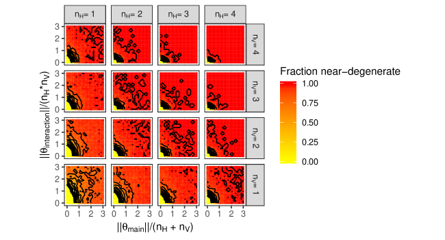
Figure 8: Results from the numerical experiment, here looking at the fraction of models that were near-degenerate for each combination of magnitudes of the points $\bm{\theta}$ and model size, where $\bm{\theta}=(\bm{\theta}_{main},\theta_{interaction})$ is split into main and interaction parameters. Black lines show the contour levels for fraction of near-degeneracy, while the thick black line shows the level where the fraction of near-degenerate models is .05.

Figure 9: The sample mean value of $\text{LREP}(\bm{\theta})/{n_{\scriptscriptstyle V}}$ at each grid point for each combination of magnitudes of the points of $\bm{\theta}$ and model size. As the magnitude of $\bm{\theta}$ grows, so does the value of this metric, indicating typical instability in the model.

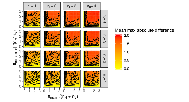
Figure 10: The sample mean of the maximum component of the absolute difference between the model expectation vector, E$\left[\bm{X}|\bm{\theta}\right]$, and the expectation vector given independence, E$\left[\bm{X}|\bm{\theta}^{*}\right]$. Larger magnitudes of $\bm{\theta}$ correspond to larger differences, thus indicating reduced interpretability.

Figure 11 shows the fraction of near-degenerate models for each magnitude of $\bm{\theta}$ for each model architecture. For each number ${n_{\scriptscriptstyle V}}$ of visibles in the model, as the number ${n_{\scriptscriptstyle H}}$ of hiddens increase, the fraction near-degenerate diverges from zero at increasing rates for larger values of $||\bm{\theta}||$. This shows that, as model size gets larger, the risk of degeneracy starts at a slightly larger magnitude of parameters, but very quickly increases until reaching close to 1.

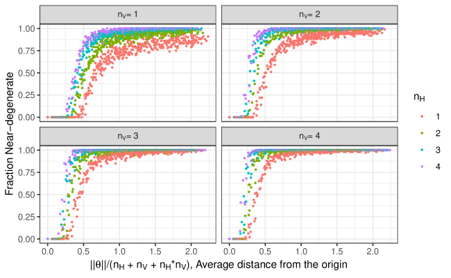
Figure 11: The fraction of near-degenerate models for each magnitude of $\bm{\theta}$. For each number ${n_{\scriptscriptstyle V}}$ of visibles in the model, the fraction near-degenerate moves away from zero at larger values of $||\bm{\theta}||$ as the number ${n_{\scriptscriptstyle H}}$ of hidden variables increases and the slope becomes steeper as ${n_{\scriptscriptstyle H}}$ increases as well.

These manageable examples indicate that RBMs are near-degenerate, unstable, and uninterpretable for large portions of the parameter space having large $\|\bm{\theta}\|$. These problematic aspects require serious consideration when using RBM models, on top of the additional matter of principled/rigorous fitting of RBM models.

4 Model Fitting

Typically, fitting a RBM via maximum likelihood (ML) methods will be unfeasible due mainly to the intractability of the normalizing term $\gamma(\bm{\theta})$ in a model (1) of any realistic size. Ad hoc methods are often recommended instead, which aim to avoid this problem by using stochastic ML approximations that employ a small number of MCMC draws (i.e., contrastive divergence, (Hinton 2002)).

However, computational concerns are not the only issues with fitting a RBM using ML. In addition, a RBM model, with the appropriate choice of parameters and number of hiddens, has the potential to re-create any distribution for the data (i.e., reproduce any specification of cell probabilities for the binary data outcomes). For example, Montufar and Ay (2011) show that any distribution on $\{0,1\}^{{n_{\scriptscriptstyle V}}}$ can be approximated arbitrarily well by a RBM with $2^{{n_{\scriptscriptstyle V}}-1}-1$ hidden units. We provide a small example in the on-line supplementary materials that illustrates such approximations.

Furthermore, as development in the online appendix shows, not only is it possible to approximate any distribution on the visibles arbitrarily well (cf. Montufar and Ay 2011), but dramatically different parameter settings can induce the same RBM model (beyond mere symmetries in parameterization). A further (and somewhat odd) consequence of the RBM parameterization is then that when fitting the RBM model by likelihood-based methods, we may already know the nature of the answer before we begin: namely, such fitting will simply reproduce the empirical distribution of the training data if sufficiently many hiddens are in the model. There then can be no model refinements or smoothing from the RBM. That is, based on a random sample of vectors of visible variables, the model for the cell probabilities with the highest likelihood over all possible model classes (i.e., RBM-based or not) is the empirical distribution, and the over-parameterization of the RBM model itself ensures that this empirical distribution can be arbitrarily well-approximated. Not only does RBM model fitting based on ML seek to reproduce the empirical distribution, whenever this empirical distribution contains empty cells, fitting steps for the RBM model will further aim to choose parameters that necessarily diverge to infinity in magnitude in order to zero-out the corresponding RBM cell probabilities. In data applications with a large sample space, it is unlikely that the training set will include at least one of each possible vector outcome (unlike this small example). This implies that some RBM model parameters must diverge to $+\infty$ to mimic the empirical distribution with empty cells and, as we have already discussed in Section 3, large magnitudes of $\bm{\theta}$ lead to model impropriety in the RBM.

Here we consider what might be done in a principled manner to prevent both overfitting and model impropriety, testing on a ${n_{\scriptscriptstyle V}}={n_{\scriptscriptstyle H}}=4$ case that already stretches the limits of what is computable — in particular we consider Bayes methods. We employ a Bayesian framework because of the ability to obtain uncertainty quantification with little to no extra effort, via posterior credible intervals.

4.1 Bayesian model fitting

To avoid model impropriety for a fitted RBM, we wish to avoid parts of the parameter space $\mathbb{R}^{{n_{\scriptscriptstyle V}}+{n_{\scriptscriptstyle H}}+{n_{\scriptscriptstyle V}}*{n_{\scriptscriptstyle H}}}$ that lead to near-degeneracy, instability, and uninterpretability. Motivated by the insights in Section 3.2, one idea is to shrink $\bm{\theta}=(\bm{\theta}_{main},\bm{\theta}_{interaction})$ toward $\bm{0}$ by specifying priors that place low probability on large values of $||\bm{\theta}||$, specifically focusing on shrinking $\bm{\theta}_{interaction}$ more than $\bm{\theta}_{main}$. This is similar to an idea advocated by Hinton (2010) called weight decay, in which a penalty is added to the interaction terms in the model, $\bm{\theta}_{interaction}$, shrinking their magnitudes.

Parameter	Value	Parameter	Value	Parameter	Value
$\theta_{v1}$	$-1.104376$	$\theta_{11}$	$-0.0006334$	$\theta_{31}$	$-0.0038301$
$\theta_{v2}$	$-0.2630044$	$\theta_{12}$	$-0.0021401$	$\theta_{32}$	$0.0032237$
$\theta_{v3}$	$0.3411915$	$\theta_{13}$	$0.0047799$	$\theta_{33}$	$0.0020681$
$\theta_{v4}$	$-0.2583769$	$\theta_{14}$	$0.0025282$	$\theta_{34}$	$0.0041429$
$\theta_{h1}$	$-0.1939302$	$\theta_{21}$	$0.0012975$	$\theta_{41}$	$0.0089533$
$\theta_{h2}$	$-0.0572858$	$\theta_{22}$	$0.0000253$	$\theta_{42}$	$-0.0042403$
$\theta_{h3}$	$-0.2101802$	$\theta_{23}$	$-0.0004352$	$\theta_{43}$	$-0.000048$
$\theta_{h4}$	$0.2402456$	$\theta_{24}$	$-0.0086621$	$\theta_{44}$	$0.0004767$

Table 1: Parameters used to fit a test case with $V=H=4$. This parameter vector was chosen as a sampled value of $\bm{\theta}$ that was not near the convex hull of the sufficient statistics for a grid point in Figure 8 with $<5$% near-degeneracy.

We considered a test case with ${n_{\scriptscriptstyle V}}={n_{\scriptscriptstyle H}}=4$ and parameters given in Table 1. This parameter vector was chosen as a sampled value of $\bm{\theta}$ at which the resulting RBM model would not be clearly degenerate. We simulated $n=5,000$ realizations of visibles as a training set and fit the RBM using three Bayes methodologies. These involved the following set-ups for choice of prior distribution $\pi(\bm{\theta})$ for parameters $\bm{\theta}$.

1. A “trick” prior. Here we cancel out normalizing term in the likelihood (from $\gamma(\bm{\theta})$ in (1)) so that resulting full conditionals of $\bm{\theta}$ are multivariate Normal. Namely, this involves a prior of the form

   $$\pi(\bm{\theta})\propto\gamma(\bm{\theta})^{n}\exp\left(-\frac{1}{2C_{1}}\bm{\theta}_{main}^{\prime}\bm{\theta}_{main}-\frac{1}{2C_{2}}\bm{\theta}_{interaction}^{\prime}\bm{\theta}_{interaction}\right),\vspace{-.75cm}$$

   where

   $$\gamma(\bm{\theta})=\sum\limits_{\bm{x}\in\mathcal{C}^{{n_{\scriptscriptstyle H}}+{n_{\scriptscriptstyle V}}}}\exp\left(\sum\limits_{i=1}^{n_{\scriptscriptstyle V}}\sum\limits_{j=1}^{n_{\scriptscriptstyle H}}\theta_{ij}v_{i}h_{j}+\sum\limits_{i=1}^{V}\theta_{v_{i}}v_{i}+\sum\limits_{j=1}^{n_{\scriptscriptstyle H}}\theta_{h_{j}}h_{j}\right)$$

   for hyperparameter choices $0<C_{2}<C_{1}$. The unknown hidden variables $h_{j}$ are also directly treated as latent variables and are sampled in each MCMC iterative draw from the posterior distribution. This is the method of Li (2014). We will refer to this method as Bayes with Trick Prior and Latent Variables (BwTPLV).

2. A truncated Normal prior. Here we use independent spherical normal distributions as priors for $\bm{\theta}_{main}$ and $\bm{\theta}_{interaction}$, which are truncated at $3\sigma_{main}$ and $3\sigma_{interaction}$, respectively, based on standard deviation hyperparameters $0<\sigma_{interaction}<\sigma_{main}$. Full conditional distributions are not conjugate, and simulation from the posterior was accomplished using a geometric adaptive Metropolis Hastings step (Zhou 2014) and calculation of likelihood normalizing constant. (This computation is barely feasible for a problem of this size and would be unfeasible for larger problems.) Here the hidden variables $h_{j}$ are again carried along in the MCMC implementation as latent variables. We will refer to this method as Bayes with Truncated Normal prior and Latent Variables (BwTNLV).

3. A truncated Normal prior and marginalized likelihood. Here we marginalize out the hidden variables $\bm{h}=(h_{1},\dots,h_{n_{\scriptscriptstyle H}})$ in $f_{\bm{\theta}}(\bm{x})$, and use the truncated Normal priors applied to the marginal probabilities for visible variables given by

   $$g_{\bm{\theta}}(\bm{v})\propto\sum\limits_{\bm{h}\in\mathcal{C}^{n_{\scriptscriptstyle H}}}\exp\left(\sum\limits_{i=1}^{n_{\scriptscriptstyle V}}\sum\limits_{j=1}^{n_{\scriptscriptstyle H}}\theta_{ij}v_{i}h_{j}+\sum\limits_{i=1}^{n_{\scriptscriptstyle V}}\theta_{v_{i}}v_{i}+\sum\limits_{j=1}^{n_{\scriptscriptstyle H}}\theta_{h_{j}}h_{j}\right),\bm{v}\in\mathcal{C}^{n_{\scriptscriptstyle V}}.$$

   We will refer to this method as Bayes with Truncated Normal prior and Marginalized Likelihood (BwTNML).

The three fitting methods are ordered above according to computational feasibility in a real-data situation, with BwTPLV being the most computationally feasible due to conjugacy and BwTNML the least feasible due to the marginalization and need for an adaptive Metropolis Hastings step. All three methods require choosing the values of hyperparameters. In each case, we have chosen these values based on a rule of thumb that shrinks $\bm{\theta}_{interaction}$ more than $\bm{\theta}_{main}$. Additionally, BwTPLV requires additional tuning (i.e. a tuning parameter $C>0$ in Table 2) to choose $C_{1}$ and $C_{2}$, reducing its appeal. The forms used for the hyperparameters in our simulation are presented in Table 2.

Method	Hyperparameter	Value
BwTPLV	$C_{1}$	$\frac{C}{n}\frac{1}{{n_{\scriptscriptstyle H}}+{n_{\scriptscriptstyle V}}}$
	$C_{2}$	$\frac{C}{n}\frac{1}{{n_{\scriptscriptstyle H}}*{n_{\scriptscriptstyle V}}}$
BwTNLV	$\sigma^{2}_{main}$	$\frac{1}{{n_{\scriptscriptstyle H}}+{n_{\scriptscriptstyle V}}}$
	$\sigma^{2}_{interaction}$	$\frac{1}{{n_{\scriptscriptstyle H}}*{n_{\scriptscriptstyle V}}}$
BwTNML	$\sigma^{2}_{main}$	$\frac{1}{{n_{\scriptscriptstyle H}}+{n_{\scriptscriptstyle V}}}$
	$\sigma^{2}_{interaction}$	$\frac{1}{{n_{\scriptscriptstyle H}}*{n_{\scriptscriptstyle V}}}$

Table 2: The values used for the hyperparameters for all three fitting methods. A rule of thumb is imposed which decreases prior variances for the model parameters as the size of the model increases and also shrinks $\bm{\theta}_{interaction}$ more than $\bm{\theta}_{main}$. The common $C$ defining $C_{1}$ and $C_{2}$ in the BwTPLV method is chosen by tuning.

It should be noted that, due to the common prior distributions for $\bm{\theta}$, both BwTNLV (method 2 above) and BwTNML (method 3) are drawing from the same stationary posterior distribution for vectors of visibles. A fundamental difference between these two methods lies in how well these two chains mix and how quickly they arrive at the target posterior distribution. After a burn-in of 50 iterations selected by inspecting the trace plots, we assess the issue of mixing in two ways. First, the autocorrelation functions (ACF) from each posterior sample corresponding to a model probability for a visible vector outcome $\mathbf{v}=(v_{1},v_{2},v_{3},v_{4})\in\{\pm 1\}^{4}$ (i.e., computed from $\bm{\theta}$ under (1) are determined and plotted in Figure 12 with BwTNLV in black and BwTNML in red. As expected, ACF corresponding to the method (BwTNML) that marginalizes out the hidden variables from the likelihood decreases to zero at a much faster rate, indicating better mixing for the chain.

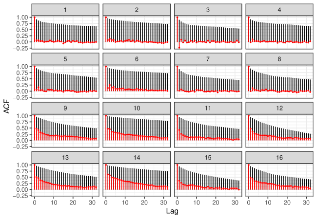
Figure 12: The autocorrelation functions (ACF) for the posterior probabilityies of all $2^{4}=16$ possible outcomes for the vector of four visibles assessed at multiple lags for each method with BwTNLV in black and BwTNML in red. As expected, ACF corresponding to the method that marginalizes out the hidden variables from the likelihood decreases to zero at a much faster rate, indicating better mixing for the chain.

Secondly, we can assess the mixing of the BwTNLV/BwTNML chains using the notion of effective sample size. If the MCMC chain were truly iid draws from the target distribution, then for the parameter $p^{(i)}$ denoting the probability of the $i$th vector outcome for the four visibles $\mathbf{v}=(v_{1},v_{2},v_{3},v_{4})\in\{\pm 1\}^{4}$, $i=1,\ldots,16$, its estimate as the average $\bar{p}^{(i)}$ of posterior sample versions would be approximately Normal with mean given by the posterior marginal mean of $p^{(i)}$, and variance given by $\sigma^{2}_{i}/M$, where $\sigma^{2}_{i}$ is the true posterior variance of $p^{(i)}$ and $M$ is the length of the chain. However, with the presence of correlation in our chain, the asymptotic variance of $\bar{p}^{(i)}$ is instead approximately some $C_{i}/M$, where $C_{i}$ is some positive constant such that $C_{i}>\sigma^{2}_{i}$. We can use an overlapping block-means approach (Gelman, Shirley, and others 2011) to get a crude estimate for $C_{i}$ as $\hat{C}_{i}=bS_{b}^{2}$, where $S_{b}^{2}$ denotes the sample variance of overlapping block means $\{\bar{p}_{j}^{(i)}=\sum_{k=j}^{j+b-1}p_{k}^{(i)}/b\}_{j=1}^{M-b+1}$ of length $b$ computed from the posterior samples $\{p_{k}^{(i)}\}_{k=1}^{M}$. We compare it to an estimate of $\sigma^{2}_{i}$ using sample variance $\hat{\sigma}^{2}_{i}$ of the raw chain, $\{p_{k}^{(i)}\}_{k=1}^{M}$. Formally, we approximate the effective sample size of the length $M$ MCMC chain as

$$M_{eff}^{(i)}=M\frac{\hat{\sigma}^{2}_{i}}{\hat{C}_{i}}.$$

Outcome	BwTNLV	BwTNML	Outcome	BwTNLV	BwTNML
1	73.00	509.43	9	83.47	394.90
2	65.05	472.51	10	95.39	327.35
3	87.10	1229.39	11	70.74	356.56
4	72.64	577.73	12	81.40	338.30
5	71.67	452.01	13	105.98	373.59
6	66.49	389.78	14	132.61	306.91
7	84.30	660.37	15	82.15	365.30
8	75.46	515.09	16	98.05	304.57

Table 3: The effective sample sizes for a chain of length $M=1000$ regarding all $16$ probabilities for possible vector outcomes of visibles. BwTNLV would require at least $4.7$ times as many MCMC iterations to achieve the same amount of effective information about the posterior distribution.

For both BwTNLV and BwTNML methods, effective sample sizes for a chain of length $M=1000$ for inference about each of the $2^{4}=16$ model probabilities are presented in Table 3. These range from $304.57$ to $1229.39$ for BwTNML, while BwTNLV only yields between $65.05$ and $132.61$ effective draws. Thus, BwTNLV would require at least $4.7$ times as many iterations of the MCMC chain to be run in order to achieve the same amount of effective information about the posterior distribution. For this reason, consistent with the ACF results in Figure 12, BwTNLV does not seem to be an effective method for fitting the RBM, though computing resources can hinder use of the alternative BwTNML involving marginalization of hidden variables.

Figure 13 shows the posterior probability of each possible $\bm{v}\in\{-1,1\}^{4}$ after fitting the RBM model according to method 1 (BwTPLV using trick prior) and method 3 (BwTNML) (excluding method 2 (BwTNLV) that seeks the same posterior as method 3) . The black vertical lines show the true probabilities of each image based on the parameters used to generate the training set while the red vertical lines show the empirical distribution for the training set of $5,000$ vectors. From these posterior predictive checks, it is evident that BwTNML produces the best fit to the data. Furthermore, along with the discussion of Section 4, Figure 13 also shows that it can be undesirable to seek to perfectly re-create an empirical distribution in fitting RBM models (i.e., true model probabilities may differ substantially). The priors in the BwTNML method constrain the RBM model fit to avoid replication of the empirical distribution and better estimate the underlying true data generating probabilities. However, this method requires a marginalization step to obtain the probability function of visible observations alone, which is unfeasible for a model with ${n_{\scriptscriptstyle H}}$ of any real size.

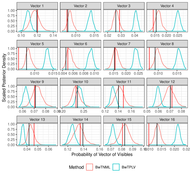
Figure 13: Posterior probabilities of $16=2^{4}$ possible realizations of $4$ visibles using two of the three Bayesian fitting techniques, BwTPLV and BwTNML. The black vertical lines show the true probabilities of each vector of visibles based on the parameters used to generate the training data while the red vertical lines show the empirical distribution. BwTNML produces the best fit for the data, however is also the most computationally intensive and least feasible with a real dataset.

An alternative possibility to using MCMC to approximate the posterior for Bayesian inference in a RBM model is to use variational methods for approximation of the posterior (Salimans, Kingma, and Welling 2015). The advantage to using variational methods would be computational scalability, but the disadvantages are potentially numerous. Namely, the lack of theoretical guarantees of convergence to a global optimum (Blei, Kucukelbir, and McAuliffe 2017) and the difficulty of assessing how closely approximated the posterior is (Yao et al. 2018) are of concern. These two issues show potential difficulties in using variational Bayes methods for interval estimation at present.

5 Discussion

RBM models constitute an interesting class of undirected graphical models that are thought to be useful for supervised learning tasks. However, when viewed as generative statistical models, RBMs can be susceptible to forms of model impropriety such as near-degeneracy, S-instability, and uninterpretability. These model instability problems relate to how useful the model may be for representing realistic data generation mechanisms. In this paper, we have provided a theoretical framework for discussing the model properties of RBMs, as well as provided empirical evidence that these model problems can arise away from the origin of the parameter space.

Additionally, these models are difficult to fit using a rigorous methodology that can incorporate estimation uncertainty, due to the dimension of the parameter space coupled with the size of the latent variable space. We have presented three fully Bayes-principled MCMC-based methods for fitting RBMs, which provide posterior distributions for quantifying uncertainty in estimating model parameters and probabilities (e.g., Figure 13) while aiming to avoid areas of the parameter space that will potentially lead to model impropriety. We have shown small examples where this fitting methodology does work, but becomes quickly intractable in large data cases.

The current common practice is to use a kind of MCMC to overcome fitting complexities, and due to the extreme flexibility in this model class, rigorous likelihood-based fitting for a RBM can typically seek to merely merely return the (discrete) empirical distribution for visibles. Current fitting methodology for RBMs does not provide uncertainty quantification for the fitted parameters, and it is unclear that they seeks to address the issues in model impropriety detailed in this paper. Practitioners should be aware of this and employ some form of regularization or penalization in the fitting.

Ultimately, it is not unquestionably clear that RBM models are useful as generative models. As a concern, without appropriate generative behavior in a RBM model, the uncertainty in estimated model parameters becomes impossible to realistically assess and the model can further lose useful application to prediction problems (e.g., realistic predictive distributions). In the case of classification, predictive distributions may not be the ultimate goal, but when S-instability is present, small (imperceptible) differences in the data may lead to greatly different probabilities and thus greatly different classifications. For these reasons, we are skeptical about RBMs as probabilistic conceptualizations for data generation.

References

Blei, David M, Alp Kucukelbir, and Jon D McAuliffe. 2017. “Variational Inference: A Review for Statisticians.” Journal of the American Statistical Association 112 (518). Taylor & Francis: 859–77.

Carreira-Perpinan, Miguel A, and Geoffrey E Hinton. 2005. “On Contrastive Divergence Learning.” In Aistats, 10:33–40.

Cho, KyungHyun, Alexander Ilin, and Tapani Raiko. 2012. “Tikhonov-Type Regularization for Restricted Boltzmann Machines.” Artificial Neural Networks and Machine Learning–ICANN 2012. Springer, 81–88.

Fisher, R. A. 1922. “On the Mathematical Foundations of Theoretical Statistics.” Philosophical Transactions of the Royal Society of London A: Mathematical, Physical and Engineering Sciences 222 (594-604). The Royal Society: 309–68.

Gelman, Andrew, Kenneth Shirley, and others. 2011. “Inference from Simulations and Monitoring Convergence.” Handbook of Markov Chain Monte Carlo, 163–74.

G. E. P. Box, W. J. Hill. 1967. “Discrimination Among Mechanistic Models.” Technometrics 9 (1). [Taylor & Francis, Ltd., American Statistical Association, American Society for Quality]: 57–71.

Handcock, Mark S. 2003. “Assessing Degeneracy in Statistical Models of Social Networks.” Center for Statistics; the Social Sciences, University of Washington. http://www.csss.washington.edu/.

Hinton, Geoffrey. 2010. “A Practical Guide to Training Restricted Boltzmann Machines.” Momentum 9 (1): 926.

Hinton, Geoffrey E. 2002. “Training Products of Experts by Minimizing Contrastive Divergence.” Neural Computation 14 (8). MIT Press: 1771–1800.

Hinton, Geoffrey E, Simon Osindero, and Yee-Whye Teh. 2006. “A Fast Learning Algorithm for Deep Belief Nets.” Neural Computation 18 (7). MIT Press: 1527–54.

Kaiser, Mark S. 2007. “Statistical Dependence in Markov Random Field Models.” Statistics Preprints Paper 57. Digital Repository @ Iowa State University. http://lib.dr.iastate.edu/stat_las_preprints/57/.

Kaplan, Andee, Daniel Nordman, and Stephen Vardeman. 2017. “On the Propriety of Restricted Boltzmann Machines.” Unpublished.

Larochelle, Hugo, and Yoshua Bengio. 2008. “Classification Using Discriminative Restricted Boltzmann Machines.” In Proceedings of the 25th International Conference on Machine Learning, 536–43. ACM.

Lehmann, E. L. 1990. “Model Specification: The Views of Fisher and Neyman, and Later Developments.” Statistical Science 5 (2). Institute of Mathematical Statistics: 160–68.

Le Roux, Nicolas, and Yoshua Bengio. 2008. “Representational Power of Restricted Boltzmann Machines and Deep Belief Networks.” Neural Computation 20 (6). MIT Press: 1631–49.

Li, Jing. 2014. “Biclustering Methods and a Bayesian Approach to Fitting Boltzmann Machines in Statistical Learning.” PhD thesis, Iowa State University; Graduate Theses; Dissertations. http://lib.dr.iastate.edu/etd/14173/.

Montufar, Guido, and Nihat Ay. 2011. “Refinements of Universal Approximation Results for Deep Belief Networks and Restricted Boltzmann Machines.” Neural Computation 23 (5). MIT Press: 1306–19.

Montúfar, Guido F, Johannes Rauh, and Nihat Ay. 2011. “Expressive Power and Approximation Errors of Restricted Boltzmann Machines.” In Advances in Neural Information Processing Systems, 415–23. NIPS.

Nguyen, Anh Mai, Jason Yosinski, and Jeff Clune. 2014. “Deep Neural Networks Are Easily Fooled: High Confidence Predictions for Unrecognizable Images.” arXiv Preprint arXiv:1412.1897. http://arxiv.org/abs/1412.1897.

Salakhutdinov, Ruslan, and Geoffrey Hinton. 2012. “An Efficient Learning Procedure for Deep Boltzmann Machines.” Neural Computation 24 (8). MIT Press: 1967–2006.

Salakhutdinov, Ruslan, and Geoffrey E Hinton. 2009. “Deep Boltzmann Machines.” In International Conference on Artificial Intelligence and Statistics, 448–55. AI & Statistics.

Salimans, Tim, Diederik Kingma, and Max Welling. 2015. “Markov Chain Monte Carlo and Variational Inference: Bridging the Gap.” In International Conference on Machine Learning, 1218–26.

Schweinberger, Michael. 2011. “Instability, Sensitivity, and Degeneracy of Discrete Exponential Families.” Journal of the American Statistical Association 106 (496). Taylor & Francis: 1361–70.

Sculley, D., Jasper Snoek, Alex Wiltschko, and Ali Rahimi. 2018. “Winner’s Curse? On Pace, Progress, and Empirical Rigor.” In 6th International Conference on Learning Representations Workshop Submission. https://openreview.net/forum?id=rJWF0Fywf.

Smolensky, Paul. 1986. “Information Processing in Dynamical Systems: Foundations of Harmony Theory.” DTIC Document.

Srivastava, Nitish, and Ruslan R Salakhutdinov. 2012. “Multimodal Learning with Deep Boltzmann Machines.” In Advances in Neural Information Processing Systems, 2222–30. NIPS.

Srivastava, Nitish, Ruslan R Salakhutdinov, and Geoffrey E Hinton. 2013. “Modeling Documents with Deep Boltzmann Machines.” arXiv Preprint arXiv:1309.6865. http://arxiv.org/abs/1309.6865.

Szegedy, Christian, Wojciech Zaremba, Ilya Sutskever, Joan Bruna, Dumitru Erhan, Ian J. Goodfellow, and Rob Fergus. 2013. “Intriguing Properties of Neural Networks.” arXiv Preprint arXiv:1312.6199. http://arxiv.org/abs/1312.6199.

Tieleman, Tijmen. 2008. “Training Restricted Boltzmann Machines Using Approximations to the Likelihood Gradient.” In Proceedings of the 25th International Conference on Machine Learning, 1064–71. ACM.

Yao, Yuling, Aki Vehtari, Daniel Simpson, and Andrew Gelman. 2018. “Yes, but Did It Work?: Evaluating Variational Inference.” In Proceedings of the 35th International Conference on Machine Learning, edited by Jennifer Dy and Andreas Krause, 80:5581–90. Proceedings of Machine Learning Research. Stockholmsmässan, Stockholm Sweden: PMLR. http://proceedings.mlr.press/v80/yao18a.html.

Zhou, Wen. 2014. “Some Bayesian and Multivariate Analysis Methods in Statistical Machine Learning and Applications.” PhD thesis, Iowa State University; Graduate Theses; Dissertations. http://lib.dr.iastate.edu/etd/13816/.