On the Pitfalls of Nested Monte Carlo

Abstract

There is an increasing interest in estimating expectations outside of the classical inference framework, such as for models expressed as probabilistic programs. Many of these contexts call for some form of nested inference to be applied. In this paper, we analyse the behaviour of nested Monte Carlo (NMC) schemes, for which classical convergence proofs are insufficient. We give conditions under which NMC will converge, establish a rate of convergence, and provide empirical data that suggests that this rate is observable in practice. Finally, we prove that general-purpose nested inference schemes are inherently biased. Our results serve to warn of the dangers associated with naïve composition of inference and models.

1 Introduction

Monte Carlo (MC) methods have become a ubiquitous means of carrying out approximate Bayesian inference. From simplistic Metropolis Hastings approaches to state-of-the-art algorithms such as the bouncy particle sampler [4] and interacting particle Markov chain MC [18], the aim of these methods is always the same: to generate approximate samples from a posterior, from which an expectation can be calculated. Although interesting alternatives have recently been suggested [5], MC integration is used almost exclusively for calculating these expectations from the produced samples.

The convergence of conventional MC integration has been covered extensively in previous literature [8, 10], but the theoretical implications arising from the nesting of MC schemes, where terms in the integrand depend on the result of a separate, nested, MC integration, have been predominantly overlooked. This paper examines convergence of such nested Monte Carlo (NMC) methods. Although we demonstrate that the construction of consistent NMC algorithms is possible, we reveal a number of associated pitfalls. In particular, NMC estimators are inherently biased, may require additional assumptions for convergence, and have significantly diminished convergence rates.

A significant motivating application for NMC occurs in the context of probabilistic programming systems (PPS) [9, 13, 15, 16, 17, 19], which allow a decoupling of model specification, in the form of a generative model with conditioning primitives, and inference, in the form of a back-end engine capable of operating on arbitrary programs. Many PPS allow for arbitrary nesting of programs so that it is easy to define and run nested inference problems, which has already begun to be exploited in application specific work [14]. However, such nesting can violate assumptions made in asserting the correctness of the underlying inference schemes. Our work highlights this issue and gives theoretical insight into the behaviour of such systems. This serves as a warning against naïve composition and a guide as to when we can expect to make reasonable estimations.

Some nested inference problems can be tackled by so-called pseudo-marginal methods [1, 2, 7, 11]. These consider cases of Bayesian inference where the likelihood is intractable, such as when it originates from an Approximate Bayesian Computation (ABC) [3, 6]. They proceed by reformulating the problem in an extended space [18], with auxiliary variables representing the stochasticity in the likelihood computation, allowing the problem to be expressed as a single expectation.

Our work goes beyond this by considering cases in which a non-linear mapping is applied to the output of the inner expectation, so that this reformulation to a single expectation is no longer possible. One scenario where this occurs is the expected information gain used in Bayesian experimental design. This requires the calculation of an entropy of a marginal distribution, and therefore includes the expectation of the logarithm of an expectation. Presuming these expectations cannot be calculated exactly, one must therefore resort to some sort of approximate nested inference scheme.

2 Problem Formulation

The idea of MC is that the expectation of an arbitrary function $\lambda\colon\mathcal{Y}\rightarrow\mathcal{F}\subseteq^{D_{f}}$ under a probability distribution $p(y)$ for its input $y\in\mathcal{Y}$ can be approximately calculated in the following fashion:

$$I =\mathbb{E}_{y\sim p(y)}\left[\lambda(y)\right]$$ (1)

$$\approx\frac{1}{N}\sum_{n=1}^{N}\lambda(y_{n})\quad\mathrm{where}\quad y_{n}\sim p(y).$$ (2)

In this paper, we consider the case where $\lambda$ is itself intractable, defined only in terms of a functional mapping of an expectation. Specifically,

$$\lambda(y)=f(y,\gamma(y))$$ (3)

where we can evaluate $f\colon\mathcal{Y}\times\Phi\rightarrow\mathcal{F}$ exactly for a given $y$ and $\gamma(y)$, but where $\gamma(y)$ is the output of an intractable expectation of another variable $z\in\mathcal{Z}$, that is,

$$\mathrm{either}\quad\gamma(y) =\mathbb{E}_{z\sim p(z|y)}\left[\phi(y,z)\right]$$ (4a)

$$\mathrm{or}\quad\gamma(y) =\mathbb{E}_{z\sim p(z)}\left[\phi(y,z)\right]$$ (4b)

depending on the problem, with $\phi\colon\mathcal{Y}\times\mathcal{Z}\rightarrow\Phi\subseteq^{D_{\phi}}$. All our results apply to both cases, but we will focus on the former for clarity. Estimating $I$ requires a nested integration. We refer to tackling both required integrations using Monte Carlo as nested Monte Carlo:

$$I\approx I_{N,M}= \frac{1}{N}\sum_{n=1}^{N}f(y_{n},(\hat{\gamma}_{M})_{n})\quad\mathrm{where}\quad y_{n}\sim p(y)\quad\mathrm{and}$$ (5a)

$$(\hat{\gamma}_{M})_{n}= \frac{1}{M}\sum_{m=1}^{M}\phi(y_{n},z_{n,m})\quad\mathrm{where}\quad z_{n,m}\sim p(z|y_{n}).$$ (5b)

The rest of this paper proceeds as follows. In Section 3, we consider a special case of $f$ that allows us to recover the standard Monte Carlo convergence rate. In Section 4, we establish convergence results for $I_{N,M}$ given a general class of $f$. In Section 5, we show that any general-purpose NMC scheme must be biased. Finally, in Section 6, we present empirical results suggesting that our theoretical convergence rates are observed in practise.

3 Reformulation to a Single Expectation

Suppose that $f$ is integrable and linear in its second argument, i.e. $f(y,\alpha v+\beta w)=\alpha f(y,v)+\beta f(y,w)$ (or equivalently $f(y,z)=g(y)z$ for some $g(y)$). In this case, we can rearrange the problem to a single expectation:

$$I=\mathbb{E}_{y\sim p(y)}\left[f(y,\gamma(y))\right] =\mathbb{E}_{y\sim p(y)}\left[f\left(y,\mathbb{E}_{z\sim p(z|y)}\left[\phi(y,z)\right]\right)\right]$$

$$=\mathbb{E}_{y\sim p(y)}\left[\mathbb{E}_{z\sim p(z|y)}\left[f(y,\phi(y,z))\right]\right]$$

$$\approx\frac{1}{N}\sum_{n=1}^{N}f(y_{n},\phi(y_{n},z_{n}))\quad\mathrm{where}\quad(y_{n},z_{n})\sim p(y)p(z|y).$$

This will give the MC convergence rate of $O(1/N)$ in the mean square error of the estimator, provided we can generate the required samples. Many models do permit this rearrangement, such as those considered by pseudo-marginal methods. Note that if $\gamma(y)$ is of the form of (4b) instead of (4a), then $y$ and $z$ are drawn independently from their marginal distributions instead of the joint.

4 Convergence of Nested Monte Carlo

Since we cannot always unravel our problem as in the previous section, we must resort to NMC in order to compute $I$ in general. Our aim here is to show that approximating $I\approx I_{N,M}$ is in principle possible, at least when $f$ is well-behaved. In particular, we prove a form of almost sure convergence of $I_{N,M}$ to $I$ and establish an upper bound on the convergence rate of its mean squared error.

To more formally characterize our conditions on $f$, consider sampling a single $y_{1}$. Then $(\hat{\gamma}_{M})_{1}=\frac{1}{M}\sum_{m=1}^{M}\phi(y_{1},z_{1,m})\rightarrow\gamma(y_{1})$ as $M\rightarrow\infty$, as the left-hand side is a Monte Carlo estimator. If $f$ is continuous around $y_{1}$, this also implies $f(y_{1},(\hat{\gamma}_{M})_{1})\rightarrow f(y_{1},\gamma(y_{1}))$. Informally, our requirement is that this holds in expectation, i.e. that it holds when we incorporate the effect of the outer estimator. More precisely, we define $(\epsilon_{M})_{n}=\left|f(y_{n},(\hat{\gamma}_{M})_{n})-f(y_{n},\gamma(y_{n}))\right|$, and require that $\mathbb{E}\left[(\epsilon_{M})_{1}\right]\to 0$ as $M\to\infty$ (noting that as $(\epsilon_{M})_{n}$ are i.i.d. $\mathbb{E}\left[(\epsilon_{M})_{1}\right]=\mathbb{E}\left[(\epsilon_{M})_{n}\right],\forall n\in\mathbb{N}$). Informally, this “expected continuity” assumption is weaker than uniform continuity as it does allow discontinuities in $f$, though we leave full characterization of intuitive criteria for $f$ to future work. We are now ready to state our theorem for almost sure convergence. Proofs for all theorems are provided in the Appendices.

Theorem 1.

For $n\in\mathbb{N}$, let $(\epsilon_{M})_{n}=\left|f(y_{n},(\hat{\gamma}_{M})_{n})-f(y_{n},\gamma(y_{n}))\right|$. If  $\mathbb{E}\left[(\epsilon_{M})_{1}\right]\to 0$ as $M\to\infty$, then there exists a $\tau:\mathbb{N}\to\mathbb{N}$ such that $I_{\tau(M),M}\overset{a.s.}{\to}I$ as $M\to\infty$.

Remark 1.

As this convergence is in $M$, it implies (and is reinforced by the convergence rate given below) that it is necessary for the number of samples in the inner estimator to increase with the number of samples in the outer estimator to ensure convergence for most $f$. Theorem 3 gives an intuitive reason for why this should be the case by noting that for finite $M$, the bias on each inner term will remain non-zero as $N\rightarrow\infty$.

Theorem 2.

If $f$ is Lipschitz continuous and $f(y_{n},\gamma(y_{n})),\phi(y_{n},z_{n,m})\in L^{2}$, then the mean squared error of $I_{N,M}$ converges at rate $O\left(1/N+1/M\right)$.

Inspection of the convergence rate above shows that, given a total number of samples $T=MN$, our bound is tightest when $\tau(M)=O(M)$ (see Section C), with a corresponding rate $O(1/\sqrt{T})$. Although Theorem 1 does not guarantee that this choice of $\tau$ converges almost surely, any other choice of $\tau$ will give a a weaker guarantee than this already problematically slow rate. Future work might consider specific forms of $\tau$ that ensure convergence.

With repeated nesting, informal extension of Theorem 2 suggests that the convergence rate will become $O(\sum_{i=1}^{d}\frac{1}{N_{i}})$ where $N_{i}$ is the number of samples used for the estimation at nesting depth $i$. This yields a bound on our convergence rate in total number of samples that becomes exponentially weaker as the total nesting depth $d$ increases. We leave a formal proof of this to future work.

5 The Inherent Bias of Nested Inference

The previous section confirmed the capabilities of NMC; in this section we establish a limitation by showing that any such general-purpose nesting scheme must be biased in the following sense:

Theorem 3.

Assume that $\gamma(y)=\mathbb{E}_{z\sim p(z|y)}[\phi(y,z)]$ is integrable as a function of $y$ but cannot be calculated exactly. Then, there does not exist a pair $(\mathcal{I},\mathcal{J})$ of inner and outer estimators such that

1. the inner estimator $\mathcal{I}$ provides estimates $\hat{\gamma}_{y}\in\Phi$ at a given $y\in\mathcal{Y}$;

2. given an integrable $f\colon\mathcal{Y}\times\Phi\rightarrow\mathcal{F}\subseteq^{D_{f}}$ the outer estimator $\mathcal{J}$ maps a set of samples $\hat{\zeta}=\left\{(y_{1},\hat{\gamma}_{y_{1}}),\dots,(y_{n},\hat{\gamma}_{y_{n}})\right\}$, with $\hat{\gamma}_{y_{i}}$ generated using $\mathcal{I}$, to an unbiased estimate $\psi(\hat{\zeta},f)$ of $I(f)$, i.e. $\mathbb{E}[\psi(\hat{\zeta},f)]=I(f)$;

3. $\mathbb{E}_{y\sim p(y)}[\mathbb{E}[f(y,\hat{\gamma}_{y})|y]]-\mathbb{E}[\psi(\hat{\zeta},f)]\geq 0$ for all integrable $f$, i.e. if $\mathcal{I}$ is combined with an exact outer estimator, there is no $f$ for which the resulting estimator is negatively biased (see Remark 2).

This result remains even if the inequality in the third condition is reversed from $ge0$ to $le0$.

Remark 2.

Informally, the first two conditions here simply provide definitions for $\mathcal{I}$ and $\mathcal{J}$ and state that they provide unbiased estimation of $I$ for all $f$. The third condition is somewhat more subtle. A simpler, but less general, alternative condition would have been to state that $\mathcal{I}$ provides unbiased estimates for any $f$, i.e. $\mathbb{E}[f(y,\hat{\gamma}_{y})|y]=f(y,\gamma(y)),\;\forall f$. The additional generality provided by the used formulation eliminates most cases in which both $\mathcal{I}$ and $\mathcal{J}$ are biased, but in such a way that these biases cancel out. Specifically, we allow $\mathcal{I}$ to be biased so long as this bias has the same sign for all $f$. As $\mathcal{I}$ and $\mathcal{J}$ are independent processes, it is intuitively reasonable to assume that $\mathcal{J}$ does not eliminate bias from $\mathcal{I}$ in a manner that is specific to $f$ and so we expect this condition to hold in practice. Future work might consider a completely general proof that also considers this case.

This result suggests that general purpose, unbiased inference is impossible for nested probabilistic program queries which cannot be mathematically expressed as single inference of the form (1). Such rearrangement is not possible when the outer query depends nonlinearly on a marginal of the inner query. Consequently, query nesting using existing systems cannot provide unbiased estimation of problems that cannot be expressed as a single query. However, the additional models that it does allow expression for, such as the experimental design example, might still be estimable in consistent fashion as shown in the previous section.

6 Empirical Verification

Strictly speaking, the convergence rates proven in Section 4 are only upper bounds on the worst case performance we can expect. We therefore provide a short empirical verification to see whether these convergence rates are tight in practice. For this, we consider the following simple model whose exact solution can be calculated:

$$y \sim\mathrm{Uniform}(-1,1)$$ (6a)

$$z \sim\mathcal{N}(0,1)$$ (6b)

$$\phi(z,y) =\sqrt{2/\pi}\exp\left(-2(y-z)^{2}\right)$$ (6c)

$$f(y,\gamma(y)) =\log(\gamma(y)).$$ (6d)

Figure 1 shows the corresponding empirical convergence obtained by applying (5) to (6) directly, and shows that, at least in this case, the theoretical convergence rates from Theorem 2 are indeed realised.

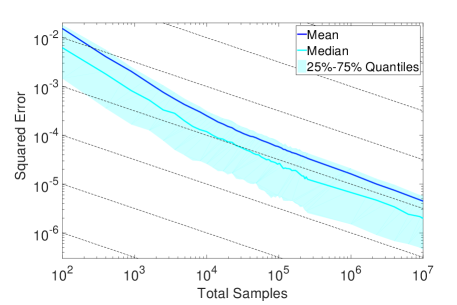
Figure 1: Empirical convergence of NMC on (6). Results are obtained by averaging over 1000 independent runs with $\tau(N)=N$ such that convergence rate obtained from Theorem 2 is $O(1/\sqrt{T})$.

7 Conclusions

We have shown that it is theoretically possible for a nested Monte Carlo scheme to yield a consistent estimator, and have quantified the convergence error associated with doing so. However, we have also revealed a number of pitfalls that can arise if nesting is applied naïvely, such as that the resulting estimator is necessarily biased, requires additional assumptions on $f$, is unlikely to converge unless the number of samples used in the inner estimator is driven to infinity, and is likely to converge at a significantly slower rate than un-nested Monte Carlo. These results have implications for applications ranging from experimental design to probabilistic programming, and serve both as an invitation for further inquiry and a caveat against careless use.

Appendix A Proof of Almost Sure Convergence (Theorem 1)

Proof.

For all $N,M$, we have by the triangle inequality that

$$\left|I_{N,M}-I\right|\leq V_{N,M}+U_{N},$$

where

$$V_{N,M} = \left|\frac{1}{N}\sum_{n=1}^{N}f(y_{n},\gamma(y_{n}))-I_{N,M}\right|$$

$$U_{N} = \left|I-\frac{1}{N}\sum_{n=1}^{N}f(y_{n},\gamma(y_{n}))\right|.$$

A second application of the triangle inequality then allows us to write

$$V_{N,M}\leq\frac{1}{N}\sum_{n=1}^{N}(\epsilon_{M})_{n}$$ (7)

where we recall that $(\epsilon_{M})_{n}=|f(y_{n},\gamma(y_{n}))-f(y_{n},\hat{\gamma}_{n})|$. Now, for all fixed $M$, each $(\epsilon_{M})_{n}$ is i.i.d, and our assumption that $\mathbb{E}\left[(\epsilon_{M})_{1}\right]\to 0$ as $M\to\infty$ ensures $\mathbb{E}\left[\left|(\epsilon_{M})_{n}\right|\right]<\infty$ for all $M$ sufficiently large. Consequently, the strong law of large numbers means that

$$\frac{1}{N}\sum_{n=1}^{N}(\epsilon_{M})_{n}\overset{a.s.}{\to}\mathbb{E}\left[(\epsilon_{M})_{1}\right]$$

as $N\to\infty$. This allows us to define $\tau_{1}:\mathbb{N}\to\mathbb{N}$ by choosing $\tau_{1}(M)$ to be large enough that

$$\left|\frac{1}{\tau_{1}(M)}\sum_{n=1}^{\tau_{1}(M)}(\epsilon_{M})_{n}-\mathbb{E}\left[(\epsilon_{M})_{1}\right]\right|<\frac{1}{M}$$

almost surely, for each $M\in\mathbb{N}$. Consequently,

$$\frac{1}{\tau_{1}(M)}\sum_{n=1}^{\tau_{1}(M)}(\epsilon_{M})_{n}<\frac{1}{M}+\mathbb{E}\left[(\epsilon_{M})_{1}\right]$$

almost surely and therefore

$$V_{\tau_{1}(M),M}<\frac{1}{M}+\mathbb{E}\left[(\epsilon_{M})_{1}\right]$$

almost surely.

To complete the proof, we must remove the dependence of $U_{N}$ on $N$ also. This is straightforward once we observe that $U_{N}\overset{a.s.}{\to}0$ as $N\to\infty$ by the strong law of large numbers, which allows us to define $\tau_{2}:\mathbb{N}\to\mathbb{N}$ by taking $\tau_{2}(M)$ large enough that

$$U_{\tau_{2}(M)}<\frac{1}{M}$$

almost surely, for each $M\in\mathbb{N}$.

We can now define $\tau(M)=\max(\tau_{1}(M),\tau_{2}(M))$. It then follows that, for all $M$,

$$\left|I-I_{\tau(M),M}\right|\leq\frac{1}{M}+\frac{1}{M}+\mathbb{E}\left[(\epsilon_{M})_{1}\right]$$

almost surely. By assumption we have $\mathbb{E}\left[(\epsilon_{M})_{1}\right]\to 0$, so that $I_{\tau(M),M}\overset{a.s.}{\to}I$ as desired.

∎

Appendix B Proof of Convergence Rate (Theorem 2)

Proof.

Using Minkowski’s inequality, we can bound the mean squared error of $I_{N,M}$ by

$$\mathbb{E}[(I-I_{N,M})^{2}]=\left\lVert I-I_{N,M}\right\rVert_{2}^{2}\leq{U}^{2}+{V}^{2}+2UV\leq 2\left(U^{2}+V^{2}\right)$$ (8)

where

$$U = \left\lVert I-\frac{1}{N}\sum_{n=1}^{N}f(y_{n},\gamma(y_{n}))\right\rVert_{2}$$

$$V = \left\lVert\frac{1}{N}\sum_{n=1}^{N}f(y_{n},\gamma(y_{n}))-I_{N,M}\right\rVert_{2}.$$

We see immediately that $U=O\left(1/\sqrt{N}\right)$, since $\frac{1}{N}\sum_{n=1}^{N}f(y_{n},\gamma(y_{n}))$ is a Monte Carlo estimator for $I$, noting our assumption that $f(y_{n},\gamma(y_{n}))\in L^{2}$. For the second term,

$$V = \left\lVert\frac{1}{N}\sum_{n=1}^{N}f(y_{n},(\hat{\gamma}_{M})_{n})-f(y_{n},\gamma(y_{n}))\right\rVert_{2}$$

$$\leq \frac{1}{N}\sum_{n=1}^{N}\left\lVert f(y_{n},(\hat{\gamma}_{M})_{n})-f(y_{n},\gamma(y_{n}))\right\rVert_{2}$$

$$\leq \frac{1}{N}\sum_{n=1}^{N}K\left\lVert(\hat{\gamma}_{M})_{n}-\gamma(y_{n})\right\rVert_{2}$$

where $K$ is a fixed constant, again by Minkowski and using the assumption that $f$ is Lipschitz. We can rewrite

$$\left\lVert(\hat{\gamma}_{M})_{n}-\gamma(y_{n})\right\rVert_{2}^{2}=\mathbb{E}\left[\mathbb{E}\left[((\hat{\gamma}_{M})_{n}-\gamma(y_{n}))^{2}\middle|y_{n}\right]\right].$$

by the tower property of conditional expectation, and note that

$$\mathbb{E}\left[((\hat{\gamma}_{M})_{n}-\gamma(y_{n}))^{2}\middle|y_{n}\right] = \operatorname*{Var}\left(\frac{1}{M}\sum_{m=1}^{M}\phi(y_{n},z_{n,m})\middle|y_{n}\right)$$

$$= \frac{1}{M}\operatorname*{Var}\left(\phi(y_{n},z_{n,1})\middle|y_{n}\right)$$

since each $z_{n,m}$ is i.i.d. and conditionally independent given $y_{n}$. As such

$$\left\lVert(\hat{\gamma}_{M})_{n}-\gamma(y_{n})\right\rVert_{2}^{2}=\frac{1}{M}\,\mathbb{E}\left[\operatorname*{Var}\left(\phi(y_{n},z_{n,1})\middle|y_{n}\right)\right]=O(1/M),$$

noting that $\mathbb{E}\left[\operatorname*{Var}\left(\phi(y_{n},z_{n,1})\middle|y_{n}\right)\right]$ is a finite constant by our assumption that $\phi(y_{n},z_{n,m})\in L^{2}$. Consequently,

$$V\leq\frac{NK}{N}O\left(1/\sqrt{M}\right)=O\left(1/\sqrt{M}\right).$$

Substituting these bounds for $U$ and $V$ in (8) gives

$$\left\lVert I-I_{N,M}\right\rVert_{2}^{2}\leq 2\left(O\left(1/\sqrt{N}\right)^{2}+O\left(1/\sqrt{M}\right)^{2}\right)=O\left(1/N+1/M\right)$$

as desired. ∎

Appendix C Optimising the Convergence Rate

We have shown that the mean squared error converges at a rate $O(1/N+1/M)$. For a given choice of $\tau$ as in Theorem 1, this becomes $O(R)$, where

$$R=1/\tau(M)+1/M.$$

Now let

$$T=\tau(M)\cdot M$$

denote the total number of samples used by our scheme. We wish to understand the relationship between $T$ and $R$.

First, suppose $\tau(M)=O(M)$ as $M\to\infty$. This easily gives

$$\frac{1}{\sqrt{\tau(M)}}=O\left(\frac{1}{\sqrt{M}}\right)$$

as $M\to\infty$, so that

$$\frac{1}{\sqrt{T}}=\frac{1}{\sqrt{M}}\frac{1}{\sqrt{\tau(M)}}=O\left(\frac{1}{M}\right)$$

and as such

$$R=O\left(\frac{1}{\sqrt{T}}\right)$$ (9)

as $M\to\infty$.

In contrast, consider the case that $M\ll\tau(M)$ as $M\to\infty$. We then have

$$\frac{1}{\sqrt{M}}\gg\frac{1}{\sqrt{\tau(M)}}$$

as $M\to\infty$, so that

$$R=O\left(\frac{1}{M}\right)\gg\frac{1}{\sqrt{M}}\frac{1}{\sqrt{\tau(M)}}=\frac{1}{\sqrt{T}}$$

as $M\to\infty$. Comparing with (9), we observe that, for the same total budget of samples $T$, this choice of $\tau$ provides a strictly weaker convergence guarantee than in the previous case. A similar argument shows that the same is true when $M\gg\tau(M)$ also.

Appendix D Proof of Inherent Bias (Theorem 3)

Proof.

For the sake of contradiction, suppose that a pair $(\mathcal{I},\mathcal{J})$ of inner and outer estimators satisfies the conditions in the theorem. Consider the possible pair of instances for $f$, $f_{1}(y,w)=(\gamma(y)-w)^{2}$ and $f_{2}(y,w)=-f_{1}(y,w)$. Since $\gamma(y)$ cannot be computed exactly by assumption, $\hat{\gamma}_{y}$ as an estimate for $\gamma(y)$ has non-zero variance. Thus, for every $y\in\mathbb{R}$, the following inequalities hold almost surely:

$$f_{1}(y,\hat{\gamma}_{y})>f_{1}(y,\gamma(y))=0=f_{2}(y,\gamma(y))>f_{2}(y,\hat{\gamma}_{y}).$$

This implies that

$$\mathbb{E}_{y\sim p(y)}\left[\mathbb{E}\left[f_{1}(y,\hat{\gamma}_{y})|y\right]\right]>0>\mathbb{E}_{y\sim p(y)}\left[\mathbb{E}\left[f_{2}(y,\hat{\gamma}_{y})|y\right]\right].$$ (10)

But

$$\mathbb{E}\left[\psi(\hat{\zeta},f_{1})\right]=I(f_{1})=0=I(f_{2})=\mathbb{E}\left[\psi(\hat{\zeta},f_{2})\right].$$ (11)

Thus,

$$\left(\mathbb{E}_{y\sim p(y)}\left[\mathbb{E}\left[f_{1}(y,\hat{\gamma}_{y})|y\right]\right]-\mathbb{E}\left[\psi(\hat{\zeta},f_{1})\right]\right)>0>\left(\mathbb{E}_{y\sim p(y)}\left[\mathbb{E}\left[f_{2}(y,\hat{\gamma}_{y})|y\right]\right]-\mathbb{E}\left[\psi(\hat{\zeta},f_{2})\right]\right).$$

This contradicts the third condition in the theorem regardless of whether we use the original $\geq 0$ or the alternative $\leq 0$. ∎

References

- Andrieu and Roberts [2009] C. Andrieu and G. O. Roberts. The pseudo-marginal approach for efficient Monte Carlo computations. The Annals of Statistics, pages 697–725, 2009.
- Andrieu et al. [2015] C. Andrieu, M. Vihola, et al. Convergence properties of pseudo-marginal Markov chain Monte Carlo algorithms. The Annals of Applied Probability, 25(2):1030–1077, 2015.
- Beaumont et al. [2002] M. A. Beaumont, W. Zhang, and D. J. Balding. Approximate Bayesian computation in population genetics. Genetics, 162(4):2025–2035, 2002.
- Bouchard-Côté et al. [2015] A. Bouchard-Côté, S. J. Vollmer, and A. Doucet. The Bouncy Particle Sampler: A Non-Reversible Rejection-Free Markov Chain Monte Carlo Method. arXiv preprint arXiv:1510.02451, 2015.
- Briol et al. [2015] F.-X. Briol, C. J. Oates, M. Girolami, M. A. Osborne, and D. Sejdinovic. Probabilistic integration: A role for statisticians in numerical analysis? arXiv preprint arXiv:1512.00933, 2015.
- Csilléry et al. [2010] K. Csilléry, M. G. Blum, O. E. Gaggiotti, and O. François. Approximate Bayesian computation (ABC) in practice. Trends in ecology & evolution, 25(7):410–418, 2010.
- Doucet et al. [2015] A. Doucet, M. Pitt, G. Deligiannidis, and R. Kohn. Efficient implementation of Markov chain Monte Carlo when using an unbiased likelihood estimator. Biometrika, page asu075, 2015.
- Gilks [2005] W. R. Gilks. Markov chain Monte Carlo. Wiley Online Library, 2005.
- Goodman et al. [2008] N. D. Goodman, V. K. Mansinghka, D. Roy, K. Bonawitz, and J. B. Tenenbaum. Church: a language for generative models. 2008.
- Huggins and Roy [2015] J. H. Huggins and D. M. Roy. Convergence of Sequential Monte Carlo-based Sampling Methods. arXiv preprint arXiv:1503.00966, 2015.
- Lindsten and Doucet [2016] F. Lindsten and A. Doucet. Pseudo-marginal Hamiltonian Monte Carlo. arXiv preprint arXiv:1607.02516, 2016.
- Lyne et al. [2015] A.-M. Lyne, M. Girolami, Y. Atchade, H. Strathmann, D. Simpson, et al. On Russian roulette estimates for Bayesian inference with doubly-intractable likelihoods. Statistical science, 30(4):443–467, 2015.
- Mansinghka et al. [2014] V. Mansinghka, D. Selsam, and Y. Perov. Venture: a higher-order probabilistic programming platform with programmable inference. arXiv preprint arXiv:1404.0099, 2014.
- Ouyang et al. [2016] L. Ouyang, M. H. Tessler, D. Ly, and N. Goodman. Practical optimal experiment design with probabilistic programs. arXiv preprint arXiv:1608.05046, 2016.
- Paige and Wood [2014] B. Paige and F. Wood. A compilation target for probabilistic programming languages. arXiv preprint arXiv:1403.0504, 2014.
- Pfeffer [2009] A. Pfeffer. Figaro: An object-oriented probabilistic programming language. Charles River Analytics Technical Report, 137, 2009.
- Rainforth et al. [2016a] T. Rainforth, T. A. Le, J.-W. van de Meent, M. A. Osborne, and F. Wood. Bayesian Optimization for Probabilistic Programs. In Advances in Neural Information Processing Systems, 2016a.
- Rainforth et al. [2016b] T. Rainforth, C. A. Naesseth, F. Lindsten, B. Paige, J.-W. van de Meent, A. Doucet, and F. Wood. Interacting particle Markov chain Monte Carlo. In Proceedings of the 33rd International Conference on Machine Learning, volume 48. JMLR: W&CP, 2016b.
- Wood et al. [2014] F. Wood, J. W. van de Meent, and V. Mansinghka. A new approach to probabilistic programming inference. In AISTATS, pages 2–46, 2014.