Spectral sum rules for conformal field theories in arbitrary dimensions

Abstract

We derive spectral sum rules in the shear channel for conformal field theories at finite temperature in general $d\geq 3$ dimensions. The sum rules result from the OPE of the stress tensor at high frequency as well as the hydrodynamic behaviour of the theory at low frequencies. The sum rule states that a weighted integral of the spectral density over frequencies is proportional to the energy density of the theory. We show that the proportionality constant can be written in terms the Hofman-Maldacena variables $t_{2},t_{4}$ which determine the three point function of the stress tensor. For theories which admit a two derivative gravity dual this proportionality constant is given by $\frac{d}{2(d+1)}$ . We then use causality constraints and obtain bounds on the sum rule which are valid in any conformal field theory. Finally we demonstrate that the high frequency behaviour of the spectral function in the vector and the tensor channel are also determined by the Hofman-Maldacena variables.

1 Introduction

Sum rules for spectral densities in any quantum field theory provide important data of the theory. The sum rule relates a weighted integral of the spectral density over frequencies to one point functions of the theory. They result because of the analyticity of the corresponding Greens function together with the short distance as well as the long distance behaviour of the theory. Thus sum rules provide useful constraints on spectral densities. For instance real time finite temperature retarded correlators are difficult to obtain from lattice calculations in QCD. However one point functions are considerably easier to obtain. This has led to a systematic study of the sum rules which constrain the spectral densities of the stress tensor in QCD Kharzeev:2007wb ; Karsch:2007jc ; Romatschke:2009ng ; Meyer:2010ii ; Meyer:2010gu . Similarly there are sum rules studied in condensed matter like the Ferrell-Golver-Tinkham sum rule which is satisfied by the current-current correlator in a BCS superconductor Ferrell:1958zza ; PhysRevLett.2.331 or the sum rule for momentum distribution in angle resolved photon emission PhysRevLett.74.4951 .

Schematically the sum rules we will focus on have the structure

$$\int_{-\infty}^{\infty}\frac{d\omega}{\omega^{n}}\rho(\omega) \propto \langle\textrm{One point functions}\rangle,$$

$$\rho(\omega) = \textrm{Im}G_{R}(\omega),$$ (1)

where $G_{R}(\omega)$ is the retarded Green’s function at finite temperature and zero momentum. As we have mentioned, sum rules are the result of the analytic properties of the Green’s function in the upper half plane which in turn follows from causality. Although sum rules primarily relate two point functions to one point functions, we will see that they contain information about the three point functions also. This information will be contained in the proportionality constant in (1).

In order to emphasise the usefulness of such rules, let us recall how such sum rules are used to determine transport properties of quark gluon plasma from the lattice. Here one postulates the form of the spectral density and then fits the parameters involved in the postulated form of the spectral density from lattice data Nakamura:2004sy ; Aarts:2007wj ; Meyer:2007ic ; Meyer:2007dy ; Huebner:2008as . Since sum rules are constraints satisfied by the spectral density, they restrict the class of the postulated form for the spectral density. For example the simplest Lorentzian anstaz for the spectral density $\frac{\omega}{\omega^{2}+\Gamma^{2}}$ is disallowed using the shear sum rules in QCD Romatschke:2009ng .

All the above properties make sum rules an important object of interest in quantum field theories. In this paper we will derive sum rules corresponding to the spectral density of the retarded correlator of the $T_{xy}$ component of the stress tensor for an arbitrary conformal field theories in $d\geq 3$ dimensions. This sum rule is usually referred to as the shear sum rule. In the context of conformal field theories, sum rules can be used to find conditions under which a certain conformal field theory admits a gravity dual. To illustrate this, we use the shear sum rule to find a necessary condition under which given conformal field theory admits a gravity dual. This condition is independent of the equality of central charges $a=c$ which is known in the literature. Sum rules together with causality can be used to find constraints both for conformal field theories as well as putative gravity duals. We will obtain these constraints in section 4 of this paper.

The investigation of sum rules in conformal field theories and its relation with holography was first done in Romatschke:2009ng . For $\mathcal{N}=4$ supersymmetric Yang-Mills theory at finite temperature the shear sum rule is given by

$$\frac{1}{\pi}\int_{-\infty}^{\infty}\frac{d\omega}{\omega}\left[\rho(\omega)-\rho_{T=0}(\omega)\right]=\frac{2}{5}\epsilon,$$ (2)

where

$$\rho(\omega)=\textrm{Im}G_{R}(\omega),$$ (3)

is the spectral density corresponding to the retarded shear correlator defined in position space by

$$G_{R}(t,\vec{x})=i\theta(t)\langle[T_{xy}(t,\vec{x}),T_{xy}(0)]\rangle.$$ (4)

The expectation value is taken in the theory held at finite temperature $T$ and $\epsilon$ in (2) is the energy density in the theory. The authors proposed the relation (2) from field theory arguments and then verified it using a holographic computation of the Greens function in the $AdS_{5}$ black hole background. The subsequent works mainly focused on the holographic derivation of the sum rules. In Gulotta:2010cu the shear sum rule was derived in holography by considering a black hole in $AdS_{d+1}$ dimensions. Modifications to the holographic shear sum rules in presence of chemical potential has been obtained in David:2011hy . This was done by considering charged blacks holes in gravitational duals of the M2, D3 and M5-brane backgrounds. The sum rules were modified due to expectation values of operators in addition to the stress tensor due to the presence of chemical potentials Similar phenomenon was investigated for sum rules corresponding to current correlators and other holographic models in David:2012cd ; WitczakKrempa:2012gn ; Katz:2014rla ; Myers:2016wsu . More recently the general structure of the shear sum rule for a conformal field theory in general dimensions was discussed in Witczak-Krempa:2015pia .

In this paper we derive the shear sum rule for an arbitrary conformal field theory in $d\geq 3$ dimensions using the general properties of conformal field theories. We consider the theory at finite temperature and at zero chemical potential. We assume that the theory is such that at finite temperature, it is only the stress tensor that acquires a non-zero expectation value. Our main result for the shear sum rule is stated as

$$\lim_{\epsilon\rightarrow 0^{+}}\frac{1}{\pi}\int_{-\infty}^{\infty}\frac{\delta\rho(\omega)d\omega}{\omega-i\epsilon} = \left(\frac{(-1+d)d}{2(1+d)}+\frac{(3-d)t_{2}}{2(-1+d)}+\frac{\left(2+3d-d^{2}\right)t_{4}}{(-1+d)(1+d)^{2}}\right)P,$$

$$\rho(z) = \textrm{Im}G_{R}(\omega),$$

$$G_{R}(t,x) = i\theta(t)[T_{xy}(t,x),T_{xy}(0)],$$

$$\delta\rho(\omega) = \rho(\omega)-\rho(\omega)_{T=0}.$$ (5)

Here $P$ refers to the pressure of the theory and $t_{2},t_{4}$ are the linearly independent parameters introduced by Hofman and Maldacena Hofman:2008ar . They carry the information of the three point function of the stress tensor and can be written in terms of the constants $a,b,c$ of Osborn:1993cr . Note that pressure can be written in terms of the energy density $\epsilon=(d-1)P$.

An immediate check on our sum rule is to apply it for theories which admit a two derivative gravity dual. From (1) we see that for these theories the sum rules reduces to

$$\lim_{\epsilon\rightarrow 0^{+}}\frac{1}{\pi}\int_{-\infty}^{\infty}\frac{\delta\rho(\omega)d\omega}{\omega-i\epsilon} = \frac{d(d-1)P}{2(d+1)}.$$ (6)

This is because $t_{2}=t_{4}=0$ for these theories. We verify this property by first explicitly using the data of the $3$ point functions of stress tensors evaluated in Arutyunov:1999nw . We then perform another check by evaluating the Greens function directly in the $AdS_{d+1}$ black hole following the methods developed in David:2011hy . Thus a necessary but not sufficient condition for a theory to admit a $2$ derivative gravity dual is that the shear sum rule given in (1) is satisfied.

Positivity of energy flux (Hofman:2008ar, ) or equivalently causality, constrains the parameters $t_{2},t_{4}$. These constraints were obtained in $d$ dimensions by Camanho:2009vw ; Buchel:2009sk and are stated in (4). Using these constraints we obtain bounds on the shear sum rule for an arbitrary conformal field theory in $d$ dimensions. We also apply the sum rules for specific theories in $d=3,4,6$. We see that for the M2-brane theory, ABJM theory, ${\cal N}=4$ Yang-Mills and the M5-brane theory, the coefficient involved in the sum rule is not renormalized as expected. For large $N$ Chern-Simons theory coupled to fundamental fermions we evaluate the coefficient involved in the sum rule as a function of the t’ Hooft coupling. We see that the bounds for the sum rule are saturated for the theory of free fermions and free bosons. As a simple application of the sum rule on obtaining constraints on theories involving higher derivatives, we obtain the bounds on the coefficient of Gauss-Bonnet gravity in arbitrary dimensions from the sum rule.

Finally we study the high frequency behavior of the spectral density in the vector and the scalar channels. That is we examine the spectral density corresponding to the correlator $\langle T_{tx}T_{xz}\rangle$ and $\langle T_{tt}T_{tt}\rangle$ respectively. We observe that the high frequency behavior is determined by Hofman-Maldacena coefficients corresponding to these channels.

The organization of the paper is as follows. In section 2 we present a general analysis of the shear sum rule we are interested in. Then we demonstrate that the high frequency behavior of the shear correlator is determined by the Hofman-Maldacena coefficient in the scalar channel and finally determine the sum rule. In section 3 we perform a consistency check on the sum rule using holography. We determine the sum rule using the evaluation of the three point function of the stress tensor in $AdS_{d+1}$ and then compare it against the direct evaluation of the sum rule from a black hole in $AdS_{d+1}$ and show agreement. In section 4 we re-write the sum rule in the Hofman-Maldacena variables $t_{2},t_{4}$ and obtain bounds on the sum rule using causality. In section 5 we discuss applications of the sum rule for well known theories in dimensions $d=3,4,6$. In section 6 we study the high frequency behavior of the retarded Greens function in the vector and the sound channel and demonstrate that that it is determined by Hofman-Maldacena coefficients in the respective channels. Section 7 contains the conclusions . Appendix A deals with the computation of the Fourier transform of the OPE coefficients in the three channels. Appendix B lists some integrals relevant for performing the Fourier transform. Finally Appendix C reviews the evaluation of the three point function of the stress tensor in Chern-Simons vector models in the large $N$ limit.

2 The shear sum rule in conformal field theories

In this section we present the derivation of the sum rule in the shear channel for conformal field theories in dimensions $d>2$. The derivation of spectral sum rules rely on the analytical properties of the Greens function in the complex $\omega$ plane. Consider a function $G(\omega)$ which is holomorphic in the upper half plane including the real axis. For the present, let us assume that the function has the following convergence property in the upper half plane

$$\lim_{\omega\rightarrow i\infty}G(\omega)\sim\frac{1}{|\omega|^{m}},\qquad m>0$$ (7)

Then using Cauchy’s theorem it can be shown that

$$G(0)=\lim_{\epsilon\rightarrow 0^{+}}\int_{-\infty}^{\infty}\frac{d\omega}{\pi}\frac{\rho(\omega)}{\omega-i\epsilon},$$ (8)

where $\rho(\omega)={\rm Im}\,G(\omega)$. We will restrict our attention to the retarded correlator of the $T_{xy}$ component of the stress tensor in $d>2$ dimensions.

$$G_{R}(t,x)=i\theta(t)\langle[T_{xy}(t,x),T_{xy}(0)]\rangle,$$ (9)

where the expectation value is taken in the theory held at finite temperature $T$. The Fourier transform is defined by

$${G_{R}}(\omega,p) = \int d^{d}xe^{i\omega t-ip.\vec{x}}G_{R}(t,x).$$ (10)

We will be interested in the sum rule for the spectral function at $p=0$, defined as

$$\rho(\omega) = \textrm{Im}{G}_{R}(\omega,0).$$ (11)

Let us now examine if each of the assumptions involved in deriving the sum rule is satisfied for the the retarded correlator. The physical reason why the retarded correlator is analytic in the upper half plane is causality. It is easy to see this from the inverse Fourier transform

$$G_{R}(t)=\int\frac{d\omega}{2\pi}e^{-i\omega t}G_{R}(\omega).$$ (12)

For $t<0$ and only when $G_{R}(\omega)$ is holomorphic, the contour can be closed in the upper half plane resulting in $G_{R}(t<0)=0$ which is a requirement for the retarded correlator. Now for conformal field theories the property (7) is not satisfied. As we will see below the retarded correlator diverges as $\lim_{\omega\rightarrow\infty}G_{R}(\omega)\sim\omega^{d}$. However we can still define a regularized Greens function $\delta G_{R}$ which satisfies the property (7) for which we can apply Cauchy’s theorem and obtain

$$\delta G_{R}(0)=\lim_{\epsilon\rightarrow 0^{+}}\int\frac{d\omega}{\pi}\frac{\delta\rho(\omega)}{\omega-i\epsilon},$$ (13)

where $\delta\rho(\omega)={\rm Im}(\delta G_{R}(\omega))$. The precise definition of the regularization of course depends on the details of the high frequency behaviour.

Thus the thing we need to do for the derivation of the sum rule is to examine the high frequency behavior of the shear correlator in the upper half plane. For this we continue $G_{R}(\omega)$ into the upper half plane using the following relation between the retarded correlator and the Euclidean correlator which can be proved from the definition of these correlators

$$G_{R}(i2\pi nT)=G_{E}(2\pi nT).$$ (14)

Here $G_{E}$ is the Euclidean time ordered correlator and $2\pi nT$ is the Matsubara frequency. This relation provides a distinguished analytic continuation

$$G_{R}(i\omega)=G_{E}(\omega).$$ (15)

We need the behavior of the retarded Greens function as $\omega\rightarrow\infty$. Consider the Euclidean correlator in position space. For time intervals $\delta t\ll\beta=\frac{1}{T}$, the operator product expansion (OPE) of the stress tensor offer a good asymptotic expansion. Therefore for $\omega\gg T$, we can replace the Euclidean correlator by its OPE. This allows us to obtain the asymptotic behaviour of the $G_{R}(i\omega)$ as $\omega\rightarrow\infty$. To conclude, the strategy is to write down the leading terms of the Euclidean OPE of the stress tensor and then Fourier transform each of these terms to frequency space to obtain the large $\omega$ behavior. Such an analysis has been used earlier in Romatschke:2009ng ; CaronHuot:2009ns ; Witczak-Krempa:2015pia .

Let us first use the OPE of the stress tensor in the Euclidean two point function. Using the result of Osborn:1993cr we obtain

$$\langle T_{xy}(s)T_{xy}(0)\rangle\sim C_{T}\frac{I_{xy,xy}(s)}{s^{2d}}+\hat{A}_{xyxy\alpha\beta}(s)\langle T_{\alpha\beta}(0)\rangle+\cdots$$ (16)

Here the OPE has been sandwiched between thermal states. $s$ refers to the position in $d$ dimensions and $C_{T}$ is a constant which determines the normalization of the $2$ point function of the stress tensor. By dimensional analysis, the tensor structure $I_{\mu\nu\rho\sigma}$ is dimensionless, while the $\hat{A}_{\mu\nu\rho\sigma}$ scales like $1/s^{d}$. From this scaling property it is easy to conclude that the following integral scales as

$$\int d^{d}xe^{i\omega t}C_{T}\frac{I_{xy,xy}(x)}{|x^{2d}|}\equiv{\cal I}\sim\omega^{d}\log(\frac{\omega}{\Lambda}),$$ (17)

where $\Lambda$ is a cut off in the integration . As we will soon see, we will not need the details of this divergent term. Lets examine the second term

$$\int_{-\infty}^{\infty}d^{d}xe^{i\omega t}\hat{A}_{xyxy\alpha\beta}(x)\langle T_{\alpha\beta}\rangle\equiv{\cal J}\sim\omega^{0}\hat{a}^{\alpha\beta}\langle T_{\alpha\beta}\rangle,$$ (18)

where $\hat{a}^{\alpha\beta}$ are $O(1)$ coefficients. For the thermal vacuum, the one point functions $\langle T_{\alpha\beta}\rangle$ can be written in terms of the energy density and the pressure. Thus these terms also contributes in the $\omega\rightarrow\infty$ limit We assume that there are no other operators of conformal dimensions $\Delta\leq d$ which gain expectation value in the thermal vacuum. The rest of the terms in the OPE (16) involve operators of dimensions $\Delta>d$ whose terms are suppressed in the $\omega\rightarrow\infty$ limit as $O(1/\omega^{\Delta-d})$.

Thus we need to regularize the retarded Greens function by subtracting ${\cal I}$ and ${\cal J}$ defined in (17) and (18). From examining ${\cal I}$, we see that it is identical to the Fourier transform of the retarded Greens function at zero temperature . Therefore we define the regularized Greens function as

$$\delta G_{R}(\omega)=G_{R}(\omega)|_{T}-G_{R}(\omega)|_{T=0}-{\cal J}.$$ (19)

Now this definition ensures that when $\omega\rightarrow i\infty$, the regularized Greens function behaves as

$$\lim_{\omega\rightarrow i\infty}\delta G_{R}(\omega)\sim O(\frac{1}{\omega^{\Delta-d}}),$$ (20)

and we can apply Cauchy’s theorem to obtain the sum rule

$$\lim_{\epsilon\rightarrow 0^{+}}\int_{-\infty}^{\infty}\frac{d\omega}{\pi}\frac{\delta\rho(\omega)}{\omega-i\epsilon} = \delta G_{R}(0),$$

$$= G_{R}(0)|_{T}-G_{R}(0)|_{T=0}-{\cal J}.$$

Now let us assume hydrodynamic behaviour of the theory at small wavelengths. This implies that we can identify the zero frequency behaviour of the retarded Greens function with pressure

$$G_{R}(0)|_{T}=P.$$ (22)

Also we have the property

$$G_{R}(0)|_{T=0}=0,$$ (23)

which arises from fact that zero temperature retarded Greens function vanish, since the pressure vanishes at zero temperature in a conformal field theory. Combining (22) and (23) we obtain the sum rule

$$\lim_{\epsilon\rightarrow 0^{+}}\int_{-\infty}^{\infty}\frac{d\omega}{\pi}\frac{\delta\rho(\omega)}{\omega-i\epsilon}=P-{\cal J},$$ (24)

where

$$\delta\rho(\omega) = {\rm Im}G_{R}(\omega)|_{T}-{\rm Im}G_{R}(\omega)|_{T=0},$$

$$= \rho(\omega)_{T}-\rho(\omega)|_{T=0}.$$

This is because ${\cal J}$ will turn out to be real and will not contribute to the spectral density. It is important to note the origin of the $2$ terms in the RHS of the sum rule (24). The first term is due to the long wave length hydrodynamic behavior of the theory, while the 2nd term is due to the short distance behavior of the theory and results from the OPE.

2.1 High frequency behavior and Hofman-Maldacena coefficient

In this section we will evaluate ${\cal J}$ for an arbitrary conformal field theory in $d$ dimensions. Lets recall its definition

$${\cal J}(\omega,p=p_{z})=\int d^{d}xe^{i\omega t-ipz}\hat{A}_{xyxyxy\alpha\beta}(x)\langle T_{\alpha\beta}\rangle,$$ (26)

where we have also introduced momentum $p=p_{z}$ along the the direction orthogonal to $x,y$ in the Fourier transform. In the end we will set $p=0$, or equivalently expand the ${\cal J}$ at $\omega\rightarrow\infty$ and extract the constant term. The only components of the expectation value of the stress tensor which are non-zero are given by

$$\langle T_{tt}\rangle=\epsilon_{E},\qquad\langle T_{ij}\rangle=P\delta_{ij},\quad i,j=2\cdots d.$$ (27)

The subscript in $\epsilon_{E}$ reminds us that that this is the energy density in the Euclidean theory We have $\epsilon_{E}=-\epsilon$ where $\epsilon$ is the energy density in the Minkowski theory. Also recall that from conformal invariance we have the relation

$$\epsilon=(d-1)P.$$ (28)

Finally the tensor structure $\hat{A}_{\mu\nu\rho\sigma}(s)$ is given by Osborn:1993cr

$$\hat{A}_{\mu\nu\rho\sigma\alpha\beta}C_{T} = \frac{(d-2)}{d+2}(4a+2b-c)H^{1}_{\alpha\beta\mu\nu\rho\sigma}(s)+\frac{1}{d}(da+b-c)H^{2}_{\alpha\beta\mu\nu\rho\sigma}(s)$$ (29)

$$-\frac{d(d-2)a-(d-2)b-2c}{d(d+2)}(H^{2}_{\mu\nu\rho\sigma\alpha\beta}(s)+H^{2}_{\rho\sigma\mu\nu\alpha\beta}(s))+\frac{2da+2b-c}{d(d-2)}H^{3}_{\alpha\beta\mu\nu\rho\sigma}(s)$$

$$-\frac{2(d-2)a-b-c}{d(d-2)}H^{4}_{\alpha\beta\mu\nu\rho\sigma}(s)-\frac{2((d-2)a-c)}{d(d-2)}(2H^{3}_{\mu\nu\rho\sigma\alpha\beta}(s)$$

$$+\frac{((d-2)(2a+b)-dc)}{d(d^{2}-4)}(H^{4}_{\mu\nu\rho\sigma\alpha\beta}+H^{4}_{\rho\sigma\mu\nu\alpha\beta})(s))$$

$$+(Ch^{5}_{\mu\nu\rho\sigma\alpha\beta}+D(\delta_{\mu\nu}h^{3}_{\rho\sigma\alpha\beta}+\delta_{\rho\sigma}h^{3}_{\mu\nu\alpha\beta}))S_{d}\delta^{d}(s),$$

$$= I_{1}+I_{2}+I_{3}+I_{4}+I_{5}+I_{6}+I_{7}+I_{8},$$

where $C_{T},C$ are functions of the parameters $a,b,c$ which determine the three point function of the stress tensor in the conformal field theory and are given by

$$C_{T}=\frac{8\pi^{\frac{d}{2}}}{\Gamma(\frac{d}{2})}\frac{(d-2)(d+3)a-2b-(d+1)c}{d(d+2)},$$ (30)

$$C=\frac{(d-2)(2a+b)-dc}{d(d+2)},\qquad S_{d}=\frac{2\pi^{\frac{d}{2}}}{\Gamma(\frac{d}{2})}.$$

The detailed evaluation of the Fourier transform to obtain ${\cal J}$ is tedious and is provided in appendix A.1. For some intuition we will present the Fourier transform of the term $I_{4}$, note that we only need the diagonal entries $\alpha=\beta$.

$$I_{4}(s) = \frac{2da+2b-c}{d(d-2)}H^{3}_{\alpha\beta xyxy}(s),\quad H^{3}_{\alpha\beta xyxy}(s)=(\partial_{\alpha}\partial_{\beta}-\frac{1}{d}\delta_{\alpha\beta}\partial^{2})\frac{1}{(t^{2}+\vec{r}^{2})^{\frac{d-2}{2}}},$$

$$I_{4}(\omega,p) = \frac{2da+2b-c}{d(d-2)}H^{3}_{\alpha\beta xyxy}(\omega,p).$$ (31)

Performing the Fourier transform we obtain

$$\sum_{i=1}^{d-1}H^{3}_{iixyxy}(\omega,p)=\frac{4\pi^{d/2}\left(d\omega^{2}-p^{2}-\omega^{2}\right)}{d\Gamma\left(\frac{d}{2}-1\right)\left(p^{2}+\omega^{2}\right)}=-H^{3}_{ttxyxy}(\omega,p).$$ (32)

Including the coefficients obtained from the expectation value of the stress tensor we obtain

$$\hat{I}_{4}(\omega,p)=\frac{(2ad+2b-c)}{d(d-2)}\left(\frac{4\pi^{d/2}\left(d\omega^{2}-p^{2}-\omega^{2}\right)}{d\Gamma\left(\frac{d}{2}-1\right)\left(p^{2}+\omega^{2}\right)}\right)(P-\epsilon_{E}).$$ (33)

At the end we need to take $\hat{I}_{4}(\omega,0)$ as the contribution to ${\cal J}(\omega,0)$. Similarly we need to perform the Fourier transform for each of the terms $I_{1},\cdots I_{7}$ in (29). Let us briefly indicate the procedure involved in performing the Fourier transform. We first parametrize the spatial directions in terms of polar co-ordinates and then perform the angular integrations. We then perform the radial integration and finally the integration over time $t$. In each of the integrals involved, we have verified that that interchange of the order of the time and the radial integrations does not affect the results. The details of each of the Fourier transform is given in the appendix A.1. Thus sum of all these terms are given by

$$\sum_{l=1}^{7}\hat{I}_{l}(\omega,0)=\frac{(1-d)(a(d(d+4)-4)+d(2b-c))}{2\left(-a\left(d^{2}+d-6\right)+2b+cd+c\right)}P.$$ (34)

Here we have used $\epsilon_{E}=-(d-1)P$ to write all terms in terms of the pressure. At this point we observe that the term in (34) is proportional to the Hofman-Maldacena coefficient obtained by examining positivity of energy flux in the spin zero channel Hofman:2008ar . More precisely for arbitrary dimensions $d$ we obtain the relation

$$\sum_{l=1}^{7}\hat{I}_{l}(\omega,0)={2(1-d)}Pa_{T,0},$$ (35)

where $a_{T,0}$ is defined in equation (2.16) of Komargodski:2016gci and is given by

$$a_{T,0}=\frac{1}{4}\frac{a(d(d+4)-4)+d(2b-c)}{-a\left(d^{2}+d-6\right)+2b+cd+c}.$$ (36)

Note that Komargodski:2016gci were examining the kinematic regime of space like momenta, while we are examining the situation at vanishing spatial momenta but non-zero frequency which is relevant for the sum rule. Here we are examining the expectation value of the stress tensor in a thermal state while Komargodski:2016gci looked at the expectation value in a single particle. It is interesting that for both these situations we obtain the Hofman-Maldacena coefficient. Finally note 29 is a contact term in position space responsible for ensuring the conformal Ward identity Osborn:1993cr . Its Fourier transform is given by

$$\hat{I}_{8}(\omega,p)=\frac{((2a+b)(-2+d)-cd)P}{-2b-c(1+d)+a\left(-6+d+d^{2}\right)}.$$ (37)

Summing all the individual contributions in ${\cal J}$ we obtain

$${\cal J} = \frac{(1-d)P(a(d(d+4)-4)+d(2b-c))}{2\left(-a\left(d^{2}+d-6\right)+2b+cd+c\right)}+\frac{((2a+b)(-2+d)-cd)P}{-2b-c(1+d)+a\left(-6+d+d^{2}\right)}.$$

We are now in a position to evaluate $P-{\cal J}$ and write down the sum rule of conformal field theories in arbitrary dimensions

$$\lim_{\epsilon\rightarrow 0^{+}}\int_{-\infty}^{\infty}\frac{d\omega}{\pi}\frac{\delta\rho(\omega)}{\omega-i\epsilon}=\delta G(0),$$ (39)

$$= \frac{\left(2c+d(c+2bd-cd)+a\left(8+d\left(-6+d+d^{2}\right)\right)\right)P}{2(2b+c+cd)-2a\left(-6+d+d^{2}\right)}.$$

Let us now discuss the important assumption used in arriving at the above sum rule (39). As mentioned around equation (18) we have assumed that no other operator of dimensions $\Delta\leq d$ gains expectation value in the thermal vaccum. This assumption holds true for theories which admit a pure $AdS_{d+1}$ dual, for example ${\cal N}=4$ Yang-Mills. However if one turns on chemical potential for $R$-charges in such theories, other marginal operators are turned and and the sum rule is corrected. Such corrections modify the RHS of the sum rule and have been derived holographically in David:2011hy for the shear sum rule and David:2012cd for sum rules obeyed by current correlators. But, there are also situations in which relevant operators can be turned on, for example for the quantum Ising model in $2+1$ dimensions . In such situations one needs to subtract the expectation value of the corresponding operator multiplied by its OPE coefficient in the integrand which occurs in the LHS of the sum rule Witczak-Krempa:2015pia . Such a situation was also encountered holographically in David:2012cd for the case of M2 branes at finite R-charge. Thus these situations will necessitate the inclusion of additional terms in the sum rule. However the term in the RHS found in (39) will not be modified. We would also like to emphasise though the general structure of the term in the RHS can be argued by scaling and the OPE, we have related the constant in front the pressure term to the data of the conformal field theory.

Let us now briefly discuss the possible modifications of the sum rule for non conformal field theories of which QCD is a relevant example. In the derivation of the sum rule, there are two terms that contribute to the RHS ${\cal J}$ and $G_{R}(0)|_{T}=P$ in (24). The coefficient of the expectation value of the stress energy tensor in ${\cal J}$ just depends on the OPE coefficients of the theory at high energy. Therefore in a theory like QCD which is asymptotically free and conformal at high energies, these coefficients can be evaluated perturbatively. However the infrared term $G_{R}(0)|_{T}=P$ is much more difficult to obtain and rely on the hydrodynamic behaviour of the theory. Further more in all our manipulations especially in evaluating the one point function of the stress energy tensor we have used the relation $\epsilon=(d-1)P$ which is true only in conformal field theories. Also note that these expectation values depend on coupling and are evaluated at low energies of the theory. Thus taking these inputs in one can evaluate sum rules for non-conformal field theories. QCD is an example where such sum rules have been evaluated Romatschke:2009ng . Here one can see in the analysis , the coefficient ${\cal J}$ is evaluated perturbatively. However, there are other possible marginal operators that can gain expectation values in the thermal vacuum eg. ${\rm Tr}F^{2}$. These in principle depend on $\epsilon-3P$ and have not yet been carefully evaluated . Therefore in conclusion, the term involving the high energy there point function ${\cal J}$ in the sum rule can be obtained using a perturbative analysis, however there are usually other terms that are sensitive to the non-conformal nature of the theory and one needs to analyse them carefully.

3 Check from holography

In this section we evaluate the $\delta G_{R}(0)$, the RHS of the sum rule in (39) in holography. We do this in two different ways. First we use the values of the parameters $a,b,c$ obtained by evaluating the three point function of stress tensor from $AdS_{d+1}$ in Arutyunov:1999nw and determine $\delta G_{R}(0)$. We then evaluate $\delta G_{R}(0)$ more directly by considering a black hole in $AdS_{d+1}$ and evaluating the retarded Green’s function. In both cases the answer reduces to

$$\delta G_{R}(0)=\frac{d}{2(d+1)}\epsilon.$$ (40)

This provides a consistency check within holography of the sum rule in (39).

3.1 $\delta G_{R}(0)$ using the 3-point function of stress tensor

The parameters $a,b,c$ which determine the three point function of stress tensor evaluated in $AdS_{d+1}$ are usually given in terms of ${\cal A},{\cal B},{\cal C}$ which are linearly related to $a,b,c$ Arutyunov:1999nw ; Bastianelli:1999ab

$$a=\frac{\mathcal{A}}{8},\qquad b=\frac{\mathcal{B}-2\mathcal{A}}{8},\qquad c=\frac{\mathcal{C}}{2}.$$ (41)

The three parameters $\mathcal{A},\mathcal{B}$ and $\mathcal{C}$ in general $AdS_{d+1}$ upto the overall Newton’s constant in $d+1$ dimensions are given by (Arutyunov:1999nw, )

$$\mathcal{A} = 3\Delta_{d}a_{1},\qquad\mathcal{B}=\Delta_{d}(2a_{1}+a_{2}-2a_{3})$$

$$\mathcal{C} = \Delta_{d}(2a_{4}+a_{5}).$$ (42)

where,

$$\Delta_{d} = \frac{d\Gamma\left(d\right)}{2\pi^{d}(d-1)^{2}},\qquad a_{1}=\frac{4d^{3}}{3-3d},$$

$$a_{2} = -\frac{4\left(6+d\left(-4-6d+3d^{3}\right)\right)}{3(-1+d)},\qquad a_{3}=-\frac{2(6+d(-7+d(-6+5d)))}{3(-1+d)},$$

$$a_{4} = \frac{1}{3}\left(-1+\frac{1}{-1+d}+4d-3d^{3}\right),\qquad a_{5}=\frac{1}{3}\left(5+\frac{1}{-1+d}-5d\right).$$

Now using (3.1) we find the the parameters determining the three point function of the stress tensor are given by

$$a = -\frac{d^{4}\pi^{-d}\Gamma[d]}{4(-1+d)^{3}},$$

$$b = -\frac{d\left(1+(-3+d)d^{2}\right)\pi^{-d}\Gamma(1+d)}{4(-1+d)^{3}},$$

$$c = \frac{d^{3}(1-2(-1+d)d)\pi^{-d}\Gamma(d)}{4(-1+d)^{3}}.$$

Finally substituting these values into the coefficient $\delta G_{R}(0)$ of the sum rule given in (39) we obtain

$$\delta G_{R}(0) = \frac{\left(2c+d(c+2bd-cd)+a\left(8+d\left(-6+d+d^{2}\right)\right)\right)P}{2(2b+c+cd)-2a\left(-6+d+d^{2}\right)},$$ (45)

$$= \frac{(-1+d)dP}{2(1+d)},$$

$$= \frac{d\epsilon}{2(d+1)}.$$

Thus the relatively complicated rational expression in terms of $a,b,c$ reduces to a simple expression which just depends on the dimension $d$.

3.2 $\delta G_{R}(0)$ from the $AdS_{d+1}$ black hole

In this section we evaluate $\delta G_{R}(0)$ directly by studying the retarded Green’s function in the $AdS_{d+1}$ black hole background. This method was originally used for obtaining the holographic sum rule in $d=4$ dimensions in Romatschke:2009ng and then further in Gulotta:2010cu ; David:2011hy ; David:2012cd for other dimensions and more general situations. We will follow the systematic approach developed in David:2011hy . The geometry dual to a conformal field theory in $d$ dimensions at finite temperature $T$ is given by the Schwarzschild black hole in $AdS_{d+1}$ at the Hawking temperature $T$. The metric and the Hawking temperature is given by .

$$ds^{2} = \frac{dr^{2}}{r^{2}f(r)}+r^{2}(-f(r)^{2}dt^{2}+dx_{1}^{2}\cdots+dx_{d-1}^{2}),$$ (46)

$$f(r) = 1-\left(\frac{r^{+}}{r}\right)^{d},\qquad T=\frac{dr_{+}}{4\pi r}.$$

$r_{+}$ is the radius of the Horizon and for convenience we have set the radius of $AdS_{d+1}$ to unity. The retarded shear correlator is obtained by consider the fluctuation $\delta g_{xy}$ of the metric which is dual to the stress tensor $T_{xy}$. Let us define the fluctuation as

$$\delta g_{xy}=r^{2}\phi(r)e^{i\omega\tau}.$$ (47)

This perturbation obeys the equation of motion of a massless scalar in the background, which is given by

$$\frac{d^{2}\phi}{dr^{2}}+(\frac{d-1}{r}+\frac{F^{\prime}}{F})\frac{d\phi}{dr}+\frac{\omega^{2}}{F^{2}}\phi=0,$$ (48)

$$F=r^{2}f(r).$$ (49)

The retarded Greens function is obtained by imposing in going boundary conditions at the horizon $r_{+}$ and obtaining the solution to $\phi$ at the boundary $r\rightarrow\infty$ Son:2002sd . The Greens function is given by

$$G_{xy,xy}^{R}(\omega,T) = \hat{G}(\omega,T)+G_{\rm{counter}}(\omega,T)+G_{\rm{contact}}(T),$$

$$\hat{G}(\omega,T) = \frac{-1}{2\kappa^{2}}\lim_{r\rightarrow\infty}\frac{Fr^{d-1}\phi^{\prime}}{\phi},$$ (50)

where $\kappa$ is the gravitational coupling constant. $G_{\rm{counter}}(\omega)$ are the counter terms which are necessary to remove the $\log(r)$ divergences. These are independent of the temperature and are identical to the counter terms one needs at $T=0$. Hence they cancel on considering $\delta G_{R}(\omega)$. Now the contact term in the Greens function arises from the frequency independent term in the effective action and is given by

$$G_{\rm{contact}}(T)=P.$$ (51)

Thus on considering $\delta G_{R}(0)$, both the counter term as well as the contact term cancel. The counter terms cancel since they are temperature independent, while the contact term cancels because at zero frequency we have $\hat{G}_{R}(0,T)=P$. The terms which contribute to $\delta G_{R}(0)$ arise from the temperature dependent terms which are finite in the high frequency $\omega\rightarrow i\infty$ limit of $\hat{G}_{R}(0,T)$. This leads us to study the function $\hat{G}(\omega,T)$ as $\omega\rightarrow\infty$. It is convenient to introduce the variables

$$i\lambda=\frac{\omega}{r_{+}},\qquad y=\frac{\lambda r_{+}}{r}.$$ (52)

In these variables we are examining the limit $\lambda\rightarrow\infty$. The equation for $\phi$ becomes,

$$\frac{d^{2}\phi}{dy^{2}}-\frac{1}{f(y)y}\left(d-1+\frac{y^{d}}{\lambda^{d}}\right)\frac{d\phi}{dy}-\frac{\phi}{f^{2}(y)}=0,$$ (53)

where,

$$f(y)=1-\frac{y^{d}}{\lambda^{d}}.$$ (54)

Expanding the differential equation (53 as a a power series in $\lambda$ we obtain

$$\frac{d^{2}\phi}{dy^{2}}-(\frac{d-1}{y}+\frac{dy^{d-1}}{\lambda^{d}}+\cdots)\frac{d\phi}{dy}-(1+\frac{2y^{d}}{\lambda^{d}}+\cdots)\phi=0.$$ (55)

It’s easy to see that the leading equation in $\lambda$ is the equation of the minimally coupled scalar in pure $AdS_{d+1}$, the sub-leading terms in $\lambda$ account for the presence of the black hole. Lets us solve for the function $g_{R}(\omega)$ perturbatively in $\frac{1}{\lambda}$. We define

$$g=\frac{\phi^{\prime}(y)}{\phi(y)}=\sum_{n=0}^{\infty}\frac{g_{n}}{\lambda^{nd}}.$$ (56)

Substituting the expansion for $g$ in (55) and matching terms order by order in $\frac{1}{\lambda}$ we obtain the following equations for the leading terms.

$$g_{0}^{\prime}-g_{0}^{2}-\frac{d-1}{y}g_{0}-1=0,$$

$$g_{1}^{\prime}+(2g_{0}-\frac{d-1}{y})g_{1}-dg_{0}y^{d-1}-2y^{d}=0.$$ (57)

Note that that equation for the zeroth order term $g_{0}$ is identical to that obtained in the pure $AdS_{d+1}$ background. The two solutions to $g_{0}$, given by,

$$g_{0}^{(1)} = -\frac{K_{\frac{d-2}{2}}(y)}{K_{\frac{d}{2}}(y)},\qquad g_{0}^{(2)}=-\frac{I_{\frac{d-2}{2}}(y)}{I_{\frac{d}{2}}(y)}.$$ (58)

Now the second solution corresponds to the solution of $\phi$ which diverges at the origin $y\rightarrow\infty$. Therefore in the strict $\lambda\rightarrow\infty$ we must discard the second solution. In David:2011hy , it has been shown in detail that the second solution does not contribute to the finite term as $\lambda\rightarrow\infty$. Thus we look for the expansion of the first solution, substituting this solution into the the second equation we obtain $g_{1}^{(1)}$

$$g^{(1)}_{1} = \frac{1}{yK_{\frac{d}{2}}(y)^{2}}\int_{0}^{y}(2y^{d}+g_{0}dy^{d-1})yK_{\frac{d}{2}}(y)+\frac{C}{yK_{\frac{d}{2}}(y)^{2}},$$ (59)

where the term containing the arbitrary constant $C$ is the homogeneous solution. We set this constant to zero since the presence of $C$ makes $g^{(1)}_{1}$ grow exponentially at $y\rightarrow\infty$ and thus alters the boundary condition set by $g^{(0)}_{1}$. Therefore we have

$$g^{(1)}_{1} = \frac{1}{yK_{\frac{d}{2}}(y)^{2}}\int_{0}^{y}(-dy^{d}K_{\frac{d}{2}}(y)K_{\frac{d-2}{2}}(y)+2y^{d+1}K_{\frac{d}{2}}(y)^{2}),$$ (60)

$$= \frac{dy^{d-1}}{2}+\frac{y^{d+1}}{d+1}\left(1-\frac{K_{\frac{d+2}{2}}(y)^{2}}{K_{\frac{d}{2}}(y)^{2}}\right).$$

Here we have integrated each of the terms in the integrand by parts and then we use relations for the derivatives of the Bessel functions. Now to obtain the retarded Greens function we need the behavior of $g^{(1)}$ close to the boundary $y\rightarrow 0$, which is given by

$$\lim_{y\rightarrow 0}g^{(1)}_{1}(y)=-\frac{d(d-1)}{2(1+d)}y^{d-1}+\frac{(2+d)}{2+d-d^{2}}y^{d+1}+O(y^{d+3}).$$ (61)

Now substituting the expansion (56) into the definition of the Greens function we obtain

$$\lim_{\lambda\rightarrow\infty}\hat{G}(\omega,T)=\frac{r_{+}^{d}}{2\kappa^{2}}\lim_{y\rightarrow 0}\left(\frac{\lambda^{d}}{y^{d-1}}g_{0}^{(1)}-\frac{d(d-1)}{2(d+1)}\right)+O(\frac{1}{\lambda^{d}}),$$ (62)

where we have used the change of variables in (52) from $r$ to $y$. Note that the leading term is proportional to $(\lambda r_{+})^{d}=(-i\omega)^{d}$ and therefore independent of temperature. This term will be present also in pure $AdS_{d+1}$ and therefore will cancel on considering $\delta G_{R}(\omega)$. Thus the finite term in the high frequency limit in addition to the contact term that one needs to subtract to regularize the Greens function is the second term in (62). As we have argued before the the contact term is independent of the frequency and will cancel since $G_{R}(0)=P$. Using all these inputs we have

$$\delta G_{R}(0)=\frac{r_{+}^{d}}{2\kappa^{2}}\frac{d(d-1)}{2(d+1)}.$$ (63)

We can now rewrite this expression in terms for the field theory variables using the relation for pressure Bhattacharyya:2008mz

$$P=\frac{r_{+}^{d}}{2\kappa^{2}}.$$ (64)

This results in

$$\delta G_{R}(0)=\frac{d(d-1)}{2(d+1)}P=\frac{d}{2(d+1)}\epsilon.$$ (65)

The above result for the holographic shear sum rule was first derived in Gulotta:2010cu . The expression for $\delta G_{R}(0)$ in (65) coincides with the evaluation of $\delta G_{R}(0)$ in the previous section given in (45), which used the input from the three point function of the stress tensor evaluated holographically. However the evaluation of $\delta G_{R}(0)$ in this section did not rely on the explicit expression given in given in (39) in terms of the parameters of the three point function $a,b,c$ and therefore provides a consistency check for the general sum rule derived in (39).

4 Sum rule, Hofman-Maldacena variables, causality bounds

The sum rule in (39) is a ratio of a linear combination of the constants $a,b,c$ which determine the three point function. The variables $t_{2},t_{4}$ which were used to characterize the positive of energy flux Hofman:2008ar were also related to the ratios of linear combinations of the constants $a,b,c$. In $d$ dimensions, this relation is given by (Buchel:2009sk, )

$$t_{2} = 2\frac{(d+1)}{d}\frac{((d-2)(d+2)(d+1)\mathcal{A}+3d^{2}\mathcal{B}-4d(2d+1)\mathcal{C})}{((d-1)(d+2)\mathcal{A}-2\mathcal{B}-4(d+1)\mathcal{C})},$$

$$t_{4} = -\frac{(d+1)}{d}\frac{((d+2)(2d^{2}-3d-3)\mathcal{A}+2d^{2}(d+2)\mathcal{B}-4d(d+1)(d+2)\mathcal{C})}{((d-1)(d+2)\mathcal{A}-2\mathcal{B}-4(d+1)\mathcal{C})},$$ (66)

where ${\cal A},{\cal B},{\cal C}$ are linearly related to $a,b,c$ by (41) . Thus we have

$$t_{2} = \frac{2(1+d)(-d(c-3bd+2cd)+a(-1+d)(4+d(8+d)))}{d\left(-2b-c(1+d)+a\left(-6+d+d^{2}\right)\right)},$$

$$t_{4} = \frac{(1+d)(2+d)\left(d(c-2bd+cd)+3a\left(1+d-2d^{2}\right)\right)}{d\left(-2b-c(1+d)+a\left(-6+d+d^{2}\right)\right)}.$$ (67)

We can use (4) and re-write $\delta G_{R}(0)$ in terms of $t_{2},t_{4}$ which results in

$$\delta G_{R}(0)=\left(\frac{(-1+d)d}{2(1+d)}+\frac{(3-d)t_{2}}{2(-1+d)}+\frac{\left(2+3d-d^{2}\right)t_{4}}{(-1+d)(1+d)^{2}}\right)P.$$ (68)

In this form of the sum rule and from the result of the previous section, it is immediately clear that for $d>3$ theories which admit a holographic dual of Einstein gravity in $AdS_{d+1}$ lie at the origin in the $t_{2},t_{4}$, i.e. at $t_{2}=t_{4}=0$. However as expected for $d=3$, we have only one condition $t_{4}=0$. This reflects the fact that there are only $2$ independent parity even constants which determine the three point function of the stress tensor in $d=3$ Osborn:1993cr as opposed to $3$ for $d>3$. Therefore the fact that we obtained that the coefficient of $t_{2}$ vanishes in $d=3$ is a consistency check on our derivation of the sum rule.

We have seen that evaluation of the sum rule in a $2$ derivative theory of gravity reduces to (65). This implies that that a necessary condition for any conformal field theory to admit a Einstein gravity dual is that the shear sum rule must satisfy (65). It is interesting to examine if this necessary condition on the sum rule for Einstein gravity dual, that is

$$\delta G_{R}(0)=\frac{d(d-1)}{2(d+1)}P,$$ (69)

is independent of the necessary constraint of the equality of the $\hat{a}=\hat{c}$ central charges for $d=4$ . The equality of these central charges result in Hofman:2008ar ,.

$$\frac{\hat{a}}{\hat{c}}=\frac{9a-2b-10c}{3(14a-2b-5c)}=1.$$ (70)

This implies that we have the relation

$$33a-4b-5c=0.$$ (71)

We have assumed that $14a-2b-5c\neq 0$. Now let us examine constraint given by the condition (69) for $d=4$. We obtain the linear relation

$$-244a+68b-55c=0.$$ (72)

which is independent of (71).

Finally let us examine the implications of the positivity of energy flux Hofman:2008ar constraints on the sum rule. These constraints have been recently shown to be related to causality and unitarity of the conformal field theory Hartman:2015lfa ; Komargodski:2016gci ; Hofman:2016awc . For conformal field theories in $d>3$ dimensions, positivity of energy implies the following bounds on the parameters $t_{2},t_{4}$ Camanho:2009vw

$$1-\frac{1}{d-1}t_{2}-\frac{2}{(d+1)(d-1)}t_{4}\geq 0,$$ (73)

$$1-\frac{1}{d-1}t_{2}-\frac{2}{(d+1)(d-1)}t_{4}+\frac{1}{2}t_{2}\geq 0,$$

$$1-\frac{1}{d-1}t_{2}-\frac{2}{(d+1)(d-1)}t_{4}+\frac{d-2}{d-1}(t_{2}+t_{4})\geq 0.$$

These bounds imply that conformal field theories which obey the positivity of energy/ causality constraints lie in the region bounded by $3$ lines in the $t_{2},t_{4}$ plane. For $d=4$, this region is shown as the shaded triangle in 1.

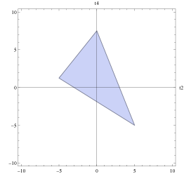
Figure 1: The allowed domain for $t_{2}$ and $t_{4}$ in $d=4$ conformal field theories.

Now given these inequalities in (73) we can obtain bounds on the function $\delta G_{R}(0)$ given in (68). The possible extrema of $\delta G_{R}(0)$ will lie on the $3$ vertices. This leads us to the following bounds on the sum rule

$$\frac{1}{2}P\leq\delta G_{R}(0)\leq\frac{d}{2}P.$$ (74)

Thus the sum rule for any conformal field theory in $d>3$ obeying the Causality bounds is constrained to lie between $\frac{P}{2}$ and and $\frac{d}{2}P$.

For $d=3$, ignoring the parity odd term in the three point function of the stress tensor found by Giombi:2011rz , it can be seen that the first inequality holds reduces to an equality Komargodski:2016gci . Therefore we obtain

$$t_{2}=2-\frac{t_{4}}{2}.$$ (75)

The remaining two inequalities reduce to

$$-4\leq t_{4}\leq 4.$$ (76)

This implies that the sum rule for parity even conformal field theories in $d=3$ is constrained to lie between

$$\frac{P}{2}\leq\delta G_{R}(0)\leq P.$$ (77)

5 Applications

The parameters $a,b$ and $c$ completely specifies the three point function of the stress tensor in a conformal field theory. In this section we will evaluate $\delta G_{R}(0)$ using the expression in (39) for well studied examples of conformal field theories in $d=3,4,6$ dimensions. All the theories that we consider here except that of Chern-Simons theory coupled to fundamental fermions have gravitational duals and are supersymmetric. We will show that for the supersymmetric theories considered here which admit a gravity dual, the coefficient in $\delta G_{R}(0)$ evaluated at at weak coupling of these theories agrees precisely with that in gravity. This strongly suggests that the sum rule is not renormalized for these theories.

5.1 $d=3$

Substituting for $d=3$ in the sum rule (39) we find that it takes the form

$$\delta G_{R}(0) = \frac{P(-13a-9b+2c)}{6a-2(b+2c)}.$$ (78)

Free conformal field theories in $d=3$ consist of $n_{s}$ real bosons and $n_{f}$ Dirac fermions. The contribution of these fields to the constants $a,b,c$ are given by Osborn:1993cr

$$a=\frac{27n_{s}}{4096\pi^{3}},\qquad b=-\frac{9(8n_{f}+9n_{s})}{4096\pi^{3}},\qquad c=-\frac{9(16n_{f}+n_{s})}{4096\pi^{3}}.$$ (79)

A well studied example of a theory in $d=3$ which admits $AdS_{4}$ as its gravity dual is that of the M2-brane. While the theory of interacting multiple M2-branes is not known, the field content of a single M2-brane is known to consist of $8$ real scalars, and 8 Majorana fermions which are equivalent to $4$ Dirac fermions. The contribution of this field content to $a,b,c$ is given by

$$a=\frac{27}{8(4\pi)^{3}},\qquad b=\frac{-117}{8(4\pi)^{3}},\qquad c=\frac{-81}{8(4\pi)^{3}}.$$ (80)

Evaluating the sum rule we obtain

$$\delta G_{R}(0)|_{\rm M2}=\frac{3P}{4}.$$ (81)

This value for the sum rule precisely agrees with that obtained in gravity for $d=3$ given in (65).

Another theory which admits $AdS_{4}$ as its gravity dual is the ABJM theory Aharony:2008ug . The values of $a,b,c$ for the interacting theory is not known. However at weak coupling, the theory consists of $3$ sets of $8$ real scalars with $N^{2}$ internal components and $3$ sets of $4$ Dirac fermions with $N^{2}$ internal components . Thus the values of $a,b,c$ for the ABJM theory is $3N^{2}$ times that of the M2-brane given in (80). The sum rule (78) is given by the ratio of these constants and remains the same as that of the M2-brane. Thus for the ABJM theory, the sum rule at weak coupling agrees precisely with the result at strong coupling.

$$\delta G_{R}(0)|_{\rm ABJM}=\frac{3P}{4}.$$ (82)

Large $N$ Chern-Simons vector theories

Recent work of Giombi:2011kc ; Aharony:2011jz ; Aharony:2012nh ; GurAri:2012is have shown that the planar limit of $U(N)$ Chern-Simons theories at level $k$ coupled to fermions or bosons in the fundamental representation are solvable in the large $N$ limit. Let us first restrict to the case of the fermionic theory. Using the analysis of MZ , it can be seen that the the three point function of the stress tensor of the interacting theory can be written as

$$\langle TTT\rangle_{\rm int\,fermion}=n_{s}(f)\langle TTT\rangle_{\rm free\,boson}+n_{f}(f)\langle TTT\rangle_{\rm free\,fermion}+\gamma(f)\langle TTT\rangle_{\rm parity\,odd},$$ (83)

where

$$n_{s}(f)=2N\frac{\sin\theta}{\theta}\sin^{2}\frac{\theta}{2},\qquad n_{f}(f)=2N\frac{\sin\theta}{\theta}\cos^{2}\frac{\theta}{2},$$ (84)

$$c(f)=N\frac{\sin^{2}\theta}{\theta},\qquad\theta=\frac{N_{f}}{k}.$$

The $f$ in the brackets refers to the fact that the theory consists of fundamental fermions and a summary of the derivation of this result is given in appendix C. The parity odd term does not play any role in the shear channel. Therefore we can treat the theory as a theory of $n_{s}(f)$ free real scalars and $n_{f}(f)$ free real fermions and therfore $\frac{n_{f}(f)}{2}$ complex fermions. Evaluating the parameters $a,b,c$ using (79) we obtain

$$a = \frac{27N\sin^{2}\left(\frac{\theta}{2}\right)\sin(\theta)}{2048\pi^{3}\theta},$$ (85)

$$b = \frac{9N\sin(\theta)(5\cos(\theta)-13)}{4096\pi^{3}\theta},$$

$$c = -\frac{9N\sin(\theta)(7\cos(\theta)+9)}{4096\pi^{3}\theta}.$$

Using these values in the sum rule (78) we obtain

$$\delta G_{R}(0)=-\frac{1}{4}P(\cos\theta-3).$$ (87)

First note that the the causality bounds for the sum rule given in (77) is satisfied as $\theta$ is dialled from $\theta=0,\cos\theta=1$ the theory of free fermions to $\theta=\pi,\cos\theta=-1$. At $\theta=\pi$, the theory of free bosons. Another interesting observation from this result for the sum rule is that at $\cos\theta=0$, the result for the sum rule agrees with that obtained from Einstein’s theory in $AdS_{4}$. The is because the theory at this point , effectively consists of $n_{f}$ free complex fermions and $n_{s}$ real scalars with $\frac{n_{s}}{n_{f}}=2$. In fact it can be seen that for any theory which satisfies $\frac{n_{s}}{n_{f}}=2$ the sum rule agrees with that in gravity. The M2-brane theory as well as the ABJM theory and other related theory which admit a gravity dual satisfies the condition $n_{s}/n_{f}=2$. It will be interesting to study if there is any simplification for the dual higher spin Vasiliev theory at $\theta=\frac{\pi}{2}$.

5.2 $d=4$

In $d=4$ The sum rule in (39) takes the following form for $d=4$.

$$\delta G_{R}(0) = \frac{P(5c-16(2a+b))}{14a-2b-5c}.$$ (88)

The values of $a,b,c$ for a theory consisting of free $n_{s}$ real scalars, $n_{f}$ Dirac fermions and $n_{v}$ vectors is given by

$$a=\frac{1}{27\pi^{6}}(n_{s}-54n_{v}),\qquad b=-\frac{1}{54\pi^{6}}(8n_{s}+27n_{f}),$$ (89)

$$c=-\frac{1}{27\pi^{6}}(n_{s}+27(n_{f}+8n_{v})).$$

Consider the case of ${\cal N}=4$ super Yang-Mills which consists of 6 real scalars, 4 Majorana fermions which is equivalent to 2 Dirac fermions and 1 vector each in the adjoint representation of the gauge group $SU(N_{c})$. Substituting these values for $n_{s},n_{f}$ and $n_{v}$ in to (89) we obtain

$$a=-\frac{16}{9\pi^{6}}(N_{c}^{2}-1),\qquad b=-\frac{17}{9\pi^{6}}(N_{c}^{2}-1),\qquad c=-\frac{92}{9\pi^{6}}(N_{c}^{2}-1).$$ (90)

With these values the sum rule (88) reduces to

$$\delta G_{R}(0)=\frac{6P}{5}.$$ (91)

which precisely agrees with the gravity result (65) for $d=4$. This result that the sum rule at weak coupling for ${\cal N}=4$ Yang-Mills agrees with that in gravity was also observed by Romatschke:2009ng .

As another consistency check for the bounds on the sum rule we have obtained in (74) let us examine the case of free $SU(N)$ Yang-Mills in $d=4$. The RHS of the shear sum rule was evaluated in Romatschke:2009ng and was shown to be $2P$ which saturates the upper bound bound in $d=4$.

5.3 $d=6$

In $d=6$, the free conformal field theories consist of $n_{s}$ real scalars, $n_{f}$ Dirac fermions and $n_{t}$, rank 2-forms. In such a theory, the values of $a,b,c$ are given by

$$a = \frac{27(-250n_{t}+n_{s})}{125\pi^{9}},$$ (92)

$$b = -\frac{18(125(6n_{t}+n_{f})+9n_{s})}{125\pi^{9}},$$

$$c = -\frac{9\left(125(96n_{t}+8n_{f})+16n_{s}\right)}{250\pi^{9}}.$$

The contribution of real scalars and Dirac fermions to the constants $a,b,c$ can be obtained from Osborn:1993cr , while the contribution of self dual tensors has been evaluated in Buchel:2009sk . The sum rule in $d=6$ takes the form,

$$\delta G_{R}(0) = -\frac{2P(56a+18b-7c)}{36a-2b-7c}.$$ (93)

The most studied theory in $d=6$ is that of the $M5$ brane which admits a holographic dual. While the theory of multiple M5-branes is not known, we can consider the theory of a single M5-brane whose field content consists of the $(2,0)$ tensor multiplet which is made up of a single self dual tensor $n_{t}=1/2$, 2 Weyl fermions which is equivalent to a single Dirac fermion and 5 real scalars. Using this field content we obtain

$$a=-\frac{2592}{100\pi^{9}},\qquad b=-\frac{7848}{100\pi^{9}},\qquad c=-\frac{25488}{100\pi^{9}}.$$ (94)

Substituting these values into the sum rule (93) we obtain

$$\delta G_{R}(0)=\frac{15P}{7}.$$ (95)

Again, the agrees with the result from gravity for $d=6$ given in (65).

5.4 Gauss Bonnet Gravity

As a simple consistency check, we will now verify that the general bounds derived for the sum rule in (74) is consistent with the existing bound on the coefficient of the coupling of the Gauss-Bonnet term in $AdS_{d+1}$ with $d\geq 4$. Bounds for the Gauss-Bonnet coupling $\lambda_{GB}$ were obtained in (Buchel:2009sk, ) using the causality bounds of Maldacena and Hofman given in in (73). From the analysis of (Buchel:2009sk, ) we obtain

$$t_{4} = 0$$

$$t_{2} = \frac{4f_{\infty}\lambda_{GB}}{1-2f_{\infty}\lambda_{GB}}\frac{(d)(d-1)}{(d-2)(d-3)}$$ (96)

where,

$$f_{\infty} = \frac{1-\sqrt{1-4\lambda_{GB}}}{2\lambda_{GB}}$$ (97)

Now causality bounds in (73) restrict the Gauss-Bonnet term to lie within

$$-\frac{(3d+2)(d-2)}{4(d+2)^{2}}\leq\lambda_{GB}\leq\frac{(d-2)(d-3)(d^{2}-d+6)}{4(d^{2}-3d+6)^{2}}$$ (98)

Let us verify that within this window of the Gauss-Bonnet coupling, the bound for the sum rule in 74 is satisfied. Substituting the values of $t_{2},t_{4}$ for Gauss-Bonnet gravity in (68) we obtain

$$\delta G(0) = \left(\frac{d(d-1)}{2(d+1)}+d\frac{\left(1-\frac{1}{\sqrt{1-4\lambda_{GB}}}\right)}{(d-2)}\right)P$$ (99)

The bounds on the Gauss-Bonnet coupling in (98) imply that

$$\left(\frac{1}{2}+\frac{1}{d+1}\right)P\leq\delta G_{GB}(0)\leq\left(\frac{d}{2}-\frac{d-1}{2(d+1)}\right)P$$ (100)

It is easy to see that this is within the general bound derived for the sum rule in (74). This result therefore serves as a minor consistency check on the coefficient of $t_{2}$ in (68) since $t_{4}$ is vanishing in Gauss-Bonnet gravity.

6 Retarded Greens function in other channels

In this section we study the high frequency behavior of the Greens function in the vector and the sound channels. We will Fourier transform the OPE in these channels and obtain the finite term. After factorizing the appropriate tensor structure in these channels we show that the finite term in these channels contains the Hofman-Maldacena coefficients

$$a_{T,1} = \frac{1}{8}\frac{d(b(2-3d)+2cd-a(-8+d(6+d)))P}{\left(-(2b+c+cd)+a\left(-6+d+d^{2}\right)\right)},$$ (101)

$$a_{T,2} = -\frac{1}{32}\frac{(4a+2b-c)(-2+d)d}{\left(-2b-c(1+d)+a\left(-6+d+d^{2}\right)\right)}.$$

6.1 The vector channel

The Greens function and its Fourier in this channel is defined by the correlator

$$G_{R;V}(t,x) = i\theta(t)\langle[T_{xt},T_{xz}]\rangle,$$ (102)

$$G_{R;V}(\omega,p_{z}) = \int d^{d}xe^{i\omega t-ip_{z}.z}i\theta(t)\langle[T_{xt},T_{xz}]\rangle.$$

As argued in the case of the shear channel, the high frequencybehavior of this Greens can be obtained by studying the OPE of the stress tensors in these channels. In the appendix A.2 we have evaluated the Fourier transform of the OPE coefficient $\hat{A}_{xtxz\alpha\beta}(\omega,p_{z})\langle T_{\alpha\beta}\rangle$. The result is given by

$$\hat{A}_{x\tau xz}(\omega,p_{z}) = -\frac{p_{z}\omega}{(p_{z}^{2}+\omega^{2})}G_{2}(\omega,p_{z}),$$ (103)

where

$$G_{2}(\omega,p_{z})=-\delta G_{R}(0)+a_{T,1}\frac{8dp_{z}^{2}}{\omega^{2}+p_{z}^{2}}P.$$ (104)

$\delta G_{R}(0)$ is the RHS of the shear sum rule defined in (39) and $a_{T,1}$ is the Hofman-Maldacena coefficient in the vector channel defined as

$$a_{T,1}=\frac{1}{8}\frac{b(2-3d)+2cd-a(-8+d(6+d))}{-(2b+c+cd)+a\left(-6+d+d^{2}\right)}.$$ (105)

It is indeed interesting that both the RHS of the shear sum rule as well as the 2nd Hofman-Maldacena coefficient appears in the high frequencybehavior in this channel. Further more note from (104), that starting from the term $(\frac{p_{z}}{\omega})^{2}$, the expansion of $G_{2}(\omega,p_{z})$ is entirely determined by the Hofman-Maldacena coefficient $a_{T,1}$. Expressed in terms of $t_{2}$ and $t_{4}$, this takes the form:

$$G_{2}(\omega,p_{z})=-\delta G_{R}(0)+\left(-\frac{4(d-3)t_{2}}{\left(d^{2}-1\right)}+\frac{16t_{4}}{(d-1)(d+1)^{2}}-\frac{8}{(d+1)}\right)\frac{dp_{z}^{2}}{p_{z}^{2}+\omega^{2}}P$$ (106)

For $d=3$, we see that the expression is independent of $t_{2}$.

For theories with a gravity dual, this becomes

$$G_{2}(\omega,p_{z})=-d\left(\frac{d-1}{2(d+1)}+\frac{8}{d+1}\frac{p_{z}^{2}}{p_{z}^{2}+\omega^{2}}\right)P,$$ (107)

which agrees with the supersymmetric examples we considered in section 5. For parity odd Chern-Simons theory coupled to fundamental matter, we expect an additional contribution from the parity-odd term in the three-point function of the stress tensor.

6.2 The sound channel

We now examine the sound channel in which the retarded Greens function and its Fourier transform is defined by

$$G_{R;S}(t,x) = i\theta(t)\langle[T_{tt},T_{tt}]\rangle$$ (108)

$$G_{R;S}(\omega,p_{z}) = \int d^{d}xe^{i\omega t-ip_{z}z}i\theta(t)\langle[T_{tt},T_{tt}]\rangle$$

The momentum is along any spatial direction. Again we can resort to the OPE to study the high frequency behavior. In the appendix (A.3) we Fourier transform the OPE coefficient corresponding to this channel and obtain

$$\hat{A}_{tttt\alpha\beta}(\omega,p_{z})\langle T_{\alpha\beta}\rangle = \frac{p_{z}^{4}}{(p_{z}^{2}+\omega^{2})^{2}}G_{3}(\omega,p_{z}).$$ (109)

The function $G_{3}(\omega,p_{z})$ admits an expansion which is given by

$$G_{3}(\omega,p_{z}) = \left(F_{1}(\frac{\omega}{p_{z}})^{4}+F_{2}(\frac{\omega}{p_{z}})^{2}+F_{3}+a_{T,2}\frac{64(\frac{p_{z}}{\omega})^{2}}{1+(\frac{p_{z}}{\omega})^{2}}\right)P.$$ (110)

Here $F_{1},F_{2},F_{3}$ are ratios of linear functions of the constants $a,b,c$. They can be written in the variables $t_{2},t_{4}$. However what is interesting is that again starting from the term $(\frac{p_{z}}{\omega})^{2}$ the entire expansion is determined by $a_{T,2}$, the Hofman-Maldacena coefficient in the tensor channel which is given by

$$a_{T,2}=-\frac{1}{32}\frac{(4a+2b-c)(-2+d)d}{\left(-2b-c(1+d)+a\left(-6+d+d^{2}\right)\right)}.$$ (111)

While the expressions for $F_{1},F_{2},F_{3}$ in terms of $a,b,c$ or $t_{2},t_{3}$ in arbitrary dimensions are fairly lengthy, we can present them for theories in $d=3$, $d=4$ and $d=6$ with a gravitational dual. We note that, while $a_{T,2}$ is independent of $t_{2}$ for $d=3$, some of the remaining terms in the expression are not independent of $t_{2}$ for $d=3$.

For $d=3$, we set $t_{2}=2$ and $t_{4}=0$, and obtain:

$$G_{3}\Big{|}_{d\rightarrow 3} = \left(\frac{32}{3}\pi-\frac{151}{18}\right)\frac{\omega^{4}}{p_{z}^{4}}P+\left({\frac{64}{3}\pi-\frac{115}{12}}\right)\frac{\omega^{2}}{p_{z}^{2}}P+\left(\frac{32\pi P}{3}-\frac{P}{36}\right)$$ (112)

$$\qquad+\frac{3p_{z}^{2}P}{8(\omega^{2}+p_{z}^{2})}$$

For $d=4$ and $d=6$, we set $t_{2}=t_{4}=0$, and obtain:

$$G_{3}\Big{|}_{d\rightarrow 4} = \left({6\pi^{2}-\frac{527}{10}}\right)\frac{\omega^{4}}{p_{z}^{4}}P+\left({12\pi^{2}-\frac{3401}{60}}\right)\frac{\omega^{2}}{p_{z}^{2}}P+\left(6\pi^{2}-\frac{131}{60}\right)P+\frac{16p_{z}^{2}P}{45(\omega^{2}+p_{z}^{2})}$$

$$G_{3}\Big{|}_{d\rightarrow 6} = \left({\frac{10}{3}\pi^{3}-\frac{8552}{63}}\right)\frac{\omega^{4}}{p_{z}^{4}}P+\left({\frac{20}{3}\pi^{3}-\frac{15046}{105}}\right)\frac{\omega^{2}}{p_{z}^{2}}P+\left(\frac{10\pi^{3}}{3}-\frac{1598}{315}\right)P$$ (113)

$$\qquad+\frac{48p_{z}^{2}P}{175(\omega^{2}+p_{z}^{2})}$$

These results agree with the supersymmetric examples of section 5.

7 Conclusions

We have derived the shear sum rule obeyed by conformal field theories in dimensions $d>0$. Assuming analyticity in the frequency plane, the sum rule holds when there are no operators of dimension $\Delta\leq d$ gain expectation value in the thermal vacuum. The RHS of the sum rule is determined by constants $a,b,c$ of the three point function of the stress tensor, these can be written in terms of the Hofman-Maldacena variables $t_{2},t_{4}$. We showed that for theories that admit a dual description in terms of Einstein gravity in $AdS_{d}$, the RHS of the sum rule reduces to $\frac{d}{2(d+1)}\epsilon$. We have also determined bounds on the sum rule using the causality constraints on $t_{2},t_{4}$. One interesting observation in the derivation of the sum rule is that the high frequency expansion of the Greens function in the shear channel is determined by the Hofman-Maldacena coefficient $a_{T,0}$ given in (36).

The shear sum rule given in (68) was cross checked by evaluating the retarded Greens function by considering a minimally coupled scalar in $AdS_{d+1}$. As one can see, this analysis only tests the coefficient independent of $t_{2},t_{4}$ in the sum rule. Note that the vanishing of the coefficient of $t_{2}$ for $d=3$ in (68) is consistent with the fact that that there is only $2$ independent parameters determining the three point function of stress tensor in $d=3$. Finally the fact that for Gauss-Bonnet gravity we have shown that the shear sum rule lies within the general bounds predicted in (74) is also a minor consistency check on the coefficient of $t_{2}$ since $t_{4}$ is vanishing in Gauss-Bonnet gravity. However it will be useful to directly check both the coefficient of $t_{2}$ and $t_{4}$ by evaluating the retarded Greens function in higher derivative theories of gravity. We hope to report on this in the near future.

We have also studied the high frequency expansion of the retarded Greens function in the vector and sound channels. We observed that again in these channels, the high frequency expansion is determined by Hofman-Maldacena coefficients $a_{T,1},a_{T,2}$ given in (101) for the vector and sound channels respectively. It will be interesting to cast this observation as sum rules in these channels and perform similar consistency checks using holography as done in this paper for the shear channel. The observation of the appearance of Hofman-Maldacena coefficients in the OPE of stress tensors have also been made in Komargodski:2016gci in the kinematic regime tuned to study deep inelastic scattering. Here the OPE is taken on an one particle state of the theory. It will be interesting to relate this to the study done in this paper where the OPE is taken in the thermal vacuum.

Finally this work points out that interesting and useful constraints on the spectral density can be obtained using conformal invariance and causality. It will be rewarding to explore this direction further.

Appendix A Fourier transform of the OPE

This appendix consists of $3$ sub-sections each of which provides the details of the Fourier transform of the tensor structure of the coefficient $\hat{A}_{\mu\nu\rho\sigma\alpha\beta}$ of the OPE of the stress tensor in $d>2$ dimensions given in (29). Section A.1 deals with the Fourier transform in the shear channel. Here the indices involved in the OPE of the two stress tensors are spatial and orthogonal to each other, the OPE considered is $\langle T_{xy}T_{xy}\rangle$. Section A.2 evaluates the Fourier transform in the vector channel where there is one spatial index common in the stress tensor and one time direction in of the stress tensor. This OPE channel is given by $\langle T_{xt}T_{xz}\rangle$. Finally in section A.3 we evaluate the Fourier transform in the sound channel given by $\langle T_{tt}T_{tt}\rangle$. In all these channels, the momentum will be taken in the $z$ direction which is orthogonal to the $x,y$ direction. However our results for the Fourier transform can be easily extended to momenta in all directions, since we have performed the basic integrals required in section B with momenta turned on in all directions.

A.1 The shear channel

Let us consider the OPE coefficient $\hat{A}_{xyxy\alpha\beta}$. We will finally require only the coefficients $\alpha=\beta$, since we take expectation values in the thermal vacuum. From Osborn:1993cr , this tensor structure is given by

$$\hat{A}_{\mu\nu\rho\sigma\alpha\beta}C_{T}=\frac{(d-2)}{d+2}(4a+2b-c)H^{1}_{\alpha\beta\mu\nu\rho\sigma}(s)+\frac{1}{d}(da+b-c)H^{2}_{\alpha\beta\mu\nu\rho\sigma}(s)$$ (114)

$$-\frac{d(d-2)a-(d-2)b-2c}{d(d+2)}(H^{2}_{\mu\nu\rho\sigma\alpha\beta}(s)+H^{2}_{\rho\sigma\mu\nu\alpha\beta}(s))+\frac{2da+2b-c}{d(d-2)}H^{3}_{\alpha\beta\mu\nu\rho\sigma}(s)$$

$$-\frac{2(d-2)a-b-c}{d(d-2)}H^{4}_{\alpha\beta\mu\nu\rho\sigma}(s)-\frac{2((d-2)a-c)}{d(d-2)}(H^{3}_{\mu\nu\rho\sigma\alpha\beta}(s)+H^{3}_{\rho\sigma\mu\nu\alpha\beta}(s))$$

$$+\frac{((d-2)(2a+b)-dc)}{d(d^{2}-4)}(H^{4}_{\mu\nu\rho\sigma\alpha\beta}+H^{4}_{\rho\sigma\mu\nu\alpha\beta})(s)$$

$$+(Ch^{5}_{\mu\nu\rho\sigma\alpha\beta}+D(\delta_{\mu\nu}h^{3}_{\rho\sigma\alpha\beta}+\delta_{\rho\sigma}h^{3}_{\mu\nu\alpha\beta}))S_{d}\delta^{d}(s),$$

$$= I_{1}+I_{2}+I_{3}+I_{4}+I_{5}+I_{6}+I_{7}+I_{8},$$

where,

$$H^{1}_{\alpha\beta xyxy}(s) = (\partial_{\alpha}\partial_{\beta}-\frac{1}{d}\delta_{\alpha\beta}\partial^{2})\left(\frac{x^{2}y^{2}}{(t^{2}+x^{2}+y^{2}+z^{2}+x_{1}^{2}+\cdots+x_{d-4}^{2})^{\frac{d+2}{2}}}\right),$$

$$H^{2}_{\alpha\beta xyxy}(s) = (\partial_{x}^{2}+\partial_{y}^{2})\frac{1}{(t^{2}+r^{2})^{\frac{d-2}{2}}}(\frac{s_{\alpha}s_{\beta}}{t^{2}+r^{2}}-\frac{1}{d}\delta_{\alpha\beta}),$$

$$H^{3}_{\alpha\beta xyxy}(s) = (\partial_{\alpha}\partial_{\beta}-\frac{1}{d}\delta_{\alpha\beta}\partial^{2})\frac{1}{(t^{2}+r^{2})^{\frac{d-2}{2}}},$$

$$H^{4}_{\alpha\beta xyxy}(s) = ((2\delta_{\alpha x}\delta_{\beta y}-\frac{2}{d}\delta_{\alpha\beta})\partial_{y}^{2}+(2\delta_{\alpha y}\delta_{\beta y}-\frac{2}{d}\delta_{\alpha\beta})\partial_{x}^{2})\frac{1}{(t^{2}+r^{2})^{\frac{d-2}{2}}},$$

$$H^{3}_{xyxy\alpha\beta}(s) = (\delta_{x\alpha}\delta_{y\beta}+\delta_{y\alpha}\delta_{x\beta})\partial_{x}\partial_{y}\frac{1}{(t^{2}+r^{2})^{\frac{d-2}{2}}},$$

$$H^{4}_{xyxy\alpha\beta}(s) = (2\delta_{y\alpha}\partial_{y}\partial_{\beta}+2\delta_{x\alpha}\partial_{x}\partial_{\beta}-\frac{2}{d}\delta_{\alpha\beta}(\partial_{y}^{2}+\partial_{x}^{2}))\frac{1}{(t^{2}+r^{2})^{\frac{d-2}{2}}},$$

$$h^{5}_{xyxy\alpha\beta} = 2\delta_{y\alpha}\delta_{y\beta}+2\delta_{x\alpha}\delta_{x\beta}-\frac{4}{d}\delta_{\alpha\beta},$$

$$C_{T} = \frac{8\pi^{\frac{d}{2}}}{\Gamma(\frac{d}{2})}\frac{(d-2)(d+3)a-2b-(d+1)c}{d(d+2)},$$

$$C = \frac{(d-2)(2a+b)-dc}{d(d+2)},\qquad S_{d}=\frac{2\pi^{\frac{d}{2}}}{\Gamma(\frac{d}{2})}.$$

To Fourier transform these tensor structures, we will first Fourier transform the tensor structures on which the derivatives act. For example for $H^{1}(s)$ defined in A.1 we will Fourier transform the expression in the curved brackets and then the action of the derivatives is obtained by inserting the appropriate momenta. We consider each of the terms $I_{i}$ with $i=1\cdots 8$ individually. For the moment, let us restrict our case for $d>3$. This is because we can find $2$ directions $x,y$ perpendicular to the momentum direction $z$. However the as we will discuss towards the end of this section we have verified that the final expression for the sum rule for $d=3$ is a natural extrapolation of the result for $d>3$ to $d=3$.

Fourier transform: $\textbf{ I}_{1}$

$$I_{1}(s) = \frac{d-2}{d+2}(4a+2b-c)H^{1}_{\alpha\beta xyxy}(s)\langle T_{\alpha\beta}(0)\rangle,$$

$$\hat{I}_{1}(\omega,p) = \frac{d-2}{d+2}(4a+2b-c)H^{1}_{\alpha\beta xyxy}(\omega,p)\langle T_{\alpha\beta}(0),\rangle$$

$$\sum_{i=1}^{d-1}H^{1}_{iixyxy}(\omega,p=p_{z}) = \left[\frac{(d-1)\left(p^{2}+\omega^{2}\right)}{d}-p^{2}\right]\times$$ (115)

$$\int d^{d}xe^{-ipz-i\omega t}\left(\frac{x^{2}y^{2}}{(t^{2}+x^{2}+y^{2}+z^{2}+x_{1}^{2}+\cdots+x_{d-4}^{2})^{\frac{d+2}{2}}}\right),$$

$$= \frac{\pi^{d/2}\left(d\omega^{2}-p^{2}-\omega^{2}\right)}{d\Gamma\left(\frac{d}{2}+1\right)\left(p^{2}+\omega^{2}\right)}.$$

Here to perform the Fourier transform we have used the integral of type 3 derived in section B. Similarly the Fourier transform for the time component is given by

$$H^{1}_{ttxyxy}(\omega,p)=-\frac{\pi^{d/2}\left(d\omega^{2}-p^{2}-\omega^{2}\right)}{d\Gamma\left(\frac{d}{2}+1\right)\left(p^{2}+\omega^{2}\right)}.$$ (116)

Thus combining these expressions along with the expectation value of the stress tensor in the thermal vacuum we obtain

$$I_{1}(\omega,p) = \frac{(d-2)(4a+2b-c)}{d+2}\frac{\pi^{d/2}\left(d\omega^{2}-p^{2}-\omega^{2}\right)}{d\Gamma\left(\frac{d}{2}+1\right)\left(p^{2}+\omega^{2}\right)}(P-\epsilon_{E}).$$ (117)

Fourier transform: $\textbf{I}_{2}$

$$I_{2}(s)=\frac{1}{d}(da+b-c)H^{2}_{\alpha\beta xyxy}(s)\langle T_{\alpha\beta}(0)\rangle$$ (118)

, $$\hat{I}_{2}(\omega,\vec{p})=\frac{1}{d}(da+b-c)H^{2}_{\alpha\beta xyxy}(\omega,\vec{p})\langle T_{\alpha\beta}(0)\rangle,$$

$$H^{2}_{\alpha\beta xyxy}(\omega,\vec{p})=(-p_{x}^{2}-p_{y}^{2})\int d^{d}xe^{-i\vec{p}\cdot\vec{r}-i\omega t}\frac{1}{(t^{2}+r^{2})^{\frac{d-2}{2}}}(\frac{s_{\alpha}s_{\beta}}{t^{2}+\vec{r}^{\,2}}-\frac{1}{d}\delta_{\alpha\beta}),$$

$$\sum_{i=1}^{d-1}H^{2}_{iixyxy}(\omega,\vec{p})=\left(-p_{x}^{2}-p_{y}^{2}\right)\left(\frac{2\pi^{d/2}\left((d-3)\left(\vec{p}^{\,2}\right)+(d-1)\omega^{2}\right)}{\Gamma\left(\frac{d}{2}\right)\left(\vec{p}^{\,2}+\omega^{2}\right)^{2}}-\frac{(d-1)\left(4\pi^{d/2}\right)}{d\left(\Gamma\left(\frac{d}{2}-1\right)\left(\vec{p}^{\,2}+\omega^{2}\right)\right)}\right).$$

Here $\vec{p}$ refers to all the spatial directions of the momentum, similarly $\vec{r}$ refers to the spatial co-ordinate. The Fourier transform has been performed using (206) and (B) Now it is clear that on taking the limit $p_{x},p_{y}\rightarrow 0$, the above expression vanishes.

$$\lim_{p_{x},p_{y}\rightarrow 0}\sum_{i=1}^{d-1}H^{2}_{iixyxy}(\omega,\vec{p})=0.$$ (119)

Similarly it can be shown that

$$\lim_{p_{x},p_{y}\rightarrow 0}H^{2}_{ttxyxy}(\omega,\vec{p})=0.$$ (120)

Therefore we obtain

$$I_{2}(\omega,p=p_{z})=0.$$ (121)

Fourier transform: $\textbf{I}_{3}$

$$I_{3}(s) = -2\frac{d(d-2)a-(d-2)b-2c}{d(d+2)}H^{2}_{xyxy\alpha\beta}(s)\langle T_{\alpha\beta}(0)\rangle,$$

$$\hat{I}_{3}(\omega,\vec{p}) = -2\frac{d(d-2)a-(d-2)b-2c}{d(d+2)}H^{2}_{xyxy\alpha\beta}(\omega,\vec{p})\langle T_{\alpha\beta}(0)\rangle,$$

$$H^{2}_{xyxyxx}(s) = H^{2}_{xyxyyy}(s)=(2-\frac{4}{d})\partial_{x}\partial_{y}\frac{xy}{(t^{2}+r^{2})^{\frac{d}{2}}},$$

$$H^{2}_{xyxyzz}(s)+\sum_{i=4}^{d-1}H^{2}_{xyxyii}(s) = -\frac{4(d-3)}{d}\partial_{x}\partial_{y}\frac{xy}{(t^{2}+r^{2})^{\frac{d}{2}}}.$$ (122)

Using these inputs and the result for the Fourier transform we obtain

$$\sum_{i=1}^{d-1}H^{2}_{xyxyii}(\omega,\vec{p}) = \frac{16\pi^{d/2}(p_{x}p_{y})^{2}}{d\Gamma\left(\frac{d}{2}\right)\left(\omega^{2}+\vec{p}^{\,2}\right)^{2}}.$$ (123)

Thus taking the limit we obtain

$$\lim_{p_{x},p_{y}\rightarrow 0}\sum_{i=1}^{d-1}H^{2}_{xyxyii}(\omega,\vec{p})=0.$$ (124)

Similarly we have

$$\lim_{p_{x},p_{y}\rightarrow 0}H^{2}_{xyxytt}(\omega,\vec{p})=0.$$ (125)

Therefore we conclude that the contribution of $\hat{I}_{3}$ vanishes.

$$\hat{I}_{3}(\omega,p=p_{z})=0.$$ (126)

Fourier transform $\textbf{I}_{4}$

$$I_{4}(s) = \frac{2da+2b-c}{d(d-2)}H^{3}_{\alpha\beta xyxy}(s),$$

$$\hat{I}_{4}(\omega,p) = \frac{2da+2b-c}{d(d-2)}H^{3}_{\alpha\beta xyxy}(\omega,p),$$

$$\sum_{i=1}^{d-1}H^{3}_{iixyxy}(\omega,p=p_{z}) = \frac{4\pi^{d/2}\left(d\omega^{2}-p^{2}-\omega^{2}\right)}{d\Gamma\left(\frac{d}{2}-1\right)\left(p^{2}+\omega^{2}\right)}.$$ (127)

Similarly we have

$$H^{3}_{ttxyxy}(\omega,p) = -\frac{4\pi^{d/2}\left(d\omega^{2}-p^{2}-\omega^{2}\right)}{d\Gamma\left(\frac{d}{2}-1\right)\left(p^{2}+\omega^{2}\right)}.$$ (128)

Therefore combining these tensor structures along with the expectation value of the stress tensor we obtain

$$\hat{I}_{4}(\omega,p=p_{z})=\frac{(2ad+2b-c)}{d(d-2)}\frac{4\pi^{d/2}\left(d\omega^{2}-p^{2}-\omega^{2}\right)}{d\Gamma\left(\frac{d}{2}-1\right)\left(p^{2}+\omega^{2}\right)}(P-\epsilon_{E}).$$ (129)

Fourier transform: $\textbf{I}_{5}$

$$I_{5}(s) = -\frac{2(d-2)a-b-c}{d(d-2)}H^{4}_{\alpha\beta xyxy}(s)\langle T_{\alpha\beta}\rangle,$$

$$\hat{I}_{5}(\omega,p) = -\frac{2(d-2)a-b-c}{d(d-2)}H^{4}_{\alpha\beta xyxy}(\omega,p)\langle T_{\alpha\beta}\rangle.$$ (130)

Now the tensor structure $H^{4}_{\alpha\beta xyxy}$ is given by

$$H^{4}_{\alpha\beta xyxy}(s) = \left[(2\delta_{\alpha x}\delta_{\beta y}-\frac{2}{d}\delta_{\alpha\beta})\partial_{y}^{2}+(2\delta_{\alpha y}\delta_{\beta y}-\frac{2}{d}\delta_{\alpha\beta})\partial_{x}^{2}\right]\frac{1}{(t^{2}+r^{2})^{\frac{d-2}{2}}}.$$ (131)

Due to the presence of the external derivatives $\partial_{x}^{2},\partial_{y}^{2}$, the Fourier transform of this tensor structure will have these derivatives replaced by $p_{x}^{2},p_{y}^{2}$ respectively. Thus in the limit $p_{x},p_{y}\rightarrow 0$, the Fourier transform vanishes and we obtain

$$H^{4}_{iixyxy}(\omega,p=p_{z})=H^{4}_{ttxyxy}(\omega,p=p_{z})=0.$$ (132)

Therefore we conclude

$$\hat{I}_{5}(\omega,p=p_{z}) = 0.$$ (133)

Fourier transform: $\textbf{I}_{6}$

$$I_{6}(s) = -\frac{2((d-2)a-c)}{d(d-2)}2H^{3}_{xyxy\alpha\beta}(s)\langle T_{\alpha\beta}\rangle,$$

$$H^{3}_{xyxy\alpha\beta}(s) = (\delta_{x\alpha}\delta_{y\beta}+\delta_{y\alpha}\delta_{x\beta})\partial_{x}\partial_{y}\frac{1}{(t^{2}+r^{2})^{\frac{d-2}{2}}}.$$ (134)

Again from the tensor structure of $H^{3}_{xyxy\alpha\beta}$, it is clear that its Fourier transform will be proportional to $p_{x}p_{y}$. Therefore in the limit $p_{x},p_{y}\rightarrow 0$, it vanishes. Thus we have

$$H^{3}_{xyxyii}(\omega,p=p_{z}) = H^{3}_{xyxytt}(\omega,p=p_{z})=0.$$

. This implies

$$\hat{I}_{6}(\omega,p=p_{z}) = 0.$$ (136)

Fourier transform: $\textbf{I}_{7}$

$$I_{7}(s) = 2\frac{((d-2)(2a+b)-dc)}{d(d^{2}-4)}(H^{4}_{xyxy\alpha\beta})(s)\langle T_{\alpha\beta}\rangle,$$

$$H^{4}_{xyxy\alpha\beta}(s) = (2\delta_{y\alpha}\partial_{y}\partial_{\beta}+2\delta_{x\alpha}\partial_{x}\partial_{\beta}-\frac{2}{d}\delta_{\alpha\beta}(\partial_{y}^{2}+\partial_{x}^{2}))\frac{1}{(t^{2}+r^{2})^{\frac{d-2}{2}}}.$$

It is clear from the tensor structure of $H^{4}_{xyxy\alpha\beta}$, that terms in the Fourier transform will always be proportional to $p_{x}$ or $p_{y}$. Therfore we have

$$H^{4}_{xyxyii}(\omega,p=p_{z})=H^{4}_{xyxytt}(\omega,p=p_{z})=0.$$ (138)

This allows us to conclude that the contribution

$$\hat{I}_{7}(\omega,p=p_{z}) = 0.$$ (139)

Fourier transform: $\textbf{I}_{8}$

The Fourier transform of the contact term $I_{8}$ leads to a constant in momentum. This is given by

$$I_{8}(s) = Ch^{5}_{xyxy\alpha\beta}S_{d}\delta^{d}(s),$$

$$h^{5}_{xyxy\alpha\beta} = 2\delta_{y\alpha}\delta_{y\beta}+2\delta_{x\alpha}\delta_{x\beta}-\frac{4}{d}\delta_{\alpha\beta}.$$

Performing this Fourier transform and also including the expectation value of the stress tensor we obtain

$$\hat{I}_{8}(\omega,p) = \frac{(d-2)(2a+b)-dc}{d^{2}(d+2)}\frac{8\pi^{d/2}}{\Gamma[d/2]}(P-\epsilon_{E}).$$ (141)

Summing up the contributions

Let us first sum up the contributions $\hat{I}_{1},\cdots\hat{I}_{7}$, that is all the terms excluding the contribution from the contact term $\hat{I}_{8}$. This leads to

$$\sum_{i=1}^{7}\hat{I}(\omega,p=p_{z})=\frac{P\left(p^{2}-(d-1)\omega^{2}\right)(a(d(d+4)-4)+d(2b-c))}{2\left(p^{2}+\omega^{2}\right)\left(-a\left(d^{2}+d-6\right)+2b+cd+c\right)}.$$ (142)

Here we have replaced the Euclidean energy $\epsilon_{E}=-(d-1)P$. Now note that this can be written as

$$\ \sum_{i=1}^{7}\hat{I}(\omega,p)=2a_{T,0}\frac{(p^{2}-(d-1)\omega^{2}}{p^{2}+\omega^{2}}P,$$ (143)

where $c_{T,0}$ is the Hofman-Maldacena coefficient in the scalar channel given in equation (2.16) of Komargodski:2016gci .

Though our analysis here has been for $d>3$, we can carry out the same steps for $d=3$, with momentum say in the $y$ direction. Now the values of Fourier transforms $\hat{I}_{1},\hat{I}_{2},\hat{I}_{4},\hat{I}_{5},\hat{I}_{7}$ are non-zero while $\hat{I}_{3},\hat{I}_{6}$ vanish However on summing up their contributions we obtain the result

$$\sum_{i=1}^{7}\hat{I}_{i}(\omega,0)=\frac{17a+6b-3c}{6a-2(b+2c)}P.$$ (144)

This is indeed the same result as that obtained by taking the $p\rightarrow 0$ limit of the expression in (142) with $d=3$.

A.2 The vector channel

We now study the Fourier transform in the vector channel. We examine the various tensor structures corresponding to the $T_{xt}T_{xz}$ OPE with momentum along the $p_{z}$ directions. Such a kinematic configuration is possible for all $d\geq 3$ dimensions.

Fourier transform: $\textbf{I}_{1}$

$$I_{1}(s) = \frac{(d-2)(4a+2b-c)}{(d+2)}H^{1}_{\alpha\beta xtxz}(s)\langle T_{\alpha\beta}(0)\rangle,$$ (145)

$$H^{1}_{\alpha\beta xtxz}(s) = (\partial_{\alpha}\partial_{\beta}-\frac{1}{d}\delta_{\alpha\beta}\partial^{2})\left(\frac{x^{2}tz}{(t^{2}+\vec{r}^{\,2})^{\frac{d+2}{2}}}\right).$$

Using the result in (213) we obtain for the Fourier transform

$$\sum_{i=1}^{d-1}H^{1}_{iixtxz}(\omega,\vec{p}) = \left(-\vec{p}^{\,2}+\frac{(d-1)}{d}(\omega^{2}+\vec{p}^{\,2})\right)\left(-\frac{2\pi^{d/2}p_{z}\omega\left(\vec{p}^{\,2}+\omega^{2}-4p_{x}^{2}\right)}{\left(\vec{p}^{\,2}+\omega^{2}\right)^{3}\Gamma\left[1+\frac{d}{2}\right]}\right).$$

Now taking the limit of all momenta to vanish except $p_{z}$ we obtain

$$\sum_{i=1}^{d-1}H^{1}_{iixtxz}(\omega,p=p_{z}) = -\frac{2\left(\pi^{d/2}p_{z}\omega\left(d\omega^{2}-p_{z}^{2}-\omega^{2}\right)\right)}{d\Gamma\left(\frac{d}{2}+1\right)\left(\omega^{2}+p_{z}^{2}\right)^{2}}.$$ (147)

Similarly for the time component we obtain

$$H^{1}_{ttxtxz}(\omega,p=p_{z}) = \frac{2\left(\pi^{d/2}p_{z}\omega\left(d\omega^{2}-p_{z}^{2}-\omega^{2}\right)\right)}{d\Gamma\left(\frac{d}{2}+1\right)\left(\omega^{2}+p_{z}^{2}\right)^{2}}.$$ (148)

Using these results and substituting the values of the expectation value of the stress tensor we obtain

$$\hat{I}_{1}(\omega,p_{z}) = \frac{(d-2)(4a+2b-c)}{d+2}\frac{2\left(\pi^{d/2}p_{z}\omega\left(d\omega^{2}-p_{z}^{2}-\omega^{2}\right)\right)}{d\Gamma\left(\frac{d}{2}+1\right)\left(\omega^{2}+p_{z}^{2}\right)^{2}}(-P+\epsilon_{E}).$$ (149)

Fourier transform: $\textbf{I}_{2}$

$$I_{2}(s) = \frac{1}{d}(da+b-c)H^{2}_{\alpha\beta xtxz}(s)\langle T_{\alpha\beta}(0)\rangle,$$

$$H^{2}_{\alpha\beta xtxz}(s) = (\partial_{z}\partial_{t})\frac{1}{(t^{2}+r^{2})^{\frac{d-2}{2}}}(\frac{s_{\alpha}s_{\beta}}{t^{2}+r^{2}}-\frac{1}{d}\delta_{\alpha\beta}).$$

We can use the result in (B) to carry out the Fourier transform. When all momenta except $p_{z}$ is set to zero we obtain

$$\sum_{i=1}^{d-1}H^{2}_{iixtxz}(\omega,p=p_{z}) = \frac{2\pi^{d/2}p_{z}\omega\left(p_{z}^{2}-(-1+d)\omega^{2}\right)}{\left(p_{z}^{2}+\omega^{2}\right)^{2}\Gamma\left[1+\frac{d}{2}\right]}.$$ (151)

Similarly for the time component we obtain

$$H^{2}_{ttxtxz}(\omega,p=p_{z}) = -\frac{2\pi^{d/2}p_{z}\omega\left(p_{z}^{2}-(-1+d)\omega^{2}\right)}{\left(p_{z}^{2}+\omega^{2}\right)^{2}\Gamma\left[1+\frac{d}{2}\right]}.$$ (152)

We can now substitute these expressions along with the expectation value of the stress tensor to obtain the Fourier transform

$$\hat{I}_{2}(\omega,p=p_{z}) = \frac{(da+b-c)}{d}\left(\frac{2\pi^{d/2}p_{z}\omega\left(p_{z}^{2}-(-1+d)\omega^{2}\right)}{\left(p_{z}^{2}+\omega^{2}\right)^{2}\Gamma\left[1+\frac{d}{2}\right]}\right)(P-\epsilon_{E}).$$ (153)

Fourier transform: $\textbf{I}_{3}$

$$I_{3}(s) = -\frac{d(d-2)a-(d-2)b-2c}{d(d+2)}(H^{2}_{xtxz\alpha\beta}(s)+H^{2}_{xzxt\alpha\beta}(s))\langle T_{\alpha\beta}(0)\rangle.$$ (154)

Now the tensor structures in $I_{3}$ are given by

$$H^{2}_{xtxz\alpha\beta}(s) = (\delta_{x\alpha}\partial_{z}\partial_{\beta}+\delta_{x\beta}\partial_{z}\partial_{\alpha}+\delta_{z\beta}\partial_{x}\partial_{\alpha}+\delta_{z\alpha}\partial_{x}\partial_{\beta}-\frac{4}{d}\delta_{\alpha\beta}\partial_{x}\partial_{z})\frac{xt}{(t^{2}+r^{2})^{\frac{d}{2}}},$$

$$H^{2}_{xzxt\alpha\beta}(s) = (\delta_{x\alpha}\partial_{t}\partial_{\beta}+\delta_{x\beta}\partial_{t}\partial_{\alpha}+\delta_{t\alpha}\partial_{x}\partial_{\beta}+\delta_{t\beta}\partial_{x}\partial_{\alpha}-\frac{4}{d}\delta_{\alpha\beta}\partial_{x}\partial_{t})\frac{xz}{(t^{2}+r^{2})^{\frac{d}{2}}}.$$

We can use (211) to Fourier transfrom these tensor structures. However it is easy to see that all of the terms which occur in the Fourier transform are proportional to momenta orthogonal to $p_{z}$. Therefore they all vanish when only $p_{z}$ is turned on which implies

$$H^{2}_{xtxz\alpha\alpha}(\omega,p=p_{z})=H^{2}_{xzxt\alpha\beta}(\omega,p=p_{z})=0.$$ (156)

Therefore we obtain

$$\hat{I}_{3}(\omega,p=p_{z})=0.$$ (157)

Fourier transform: $\textbf{I}_{4}$

$$I_{4}(s) = \frac{2da+2b-c}{d}H^{3}_{\alpha\beta xtxz}(s)\langle T_{\alpha\beta}\rangle,$$

$$H^{3}_{\alpha\beta xtxz}(s) = h^{3}_{xtxz}(\partial_{\alpha}\partial_{\beta}-\frac{1}{d}\delta_{\alpha\beta}\partial^{2})\frac{1}{(t^{2}+r^{2})^{\frac{d-2}{2}}}.$$ (158)

Now $h^{3}$ is defined as

$$h^{3}_{\mu\nu\rho\sigma}=\delta_{\mu\rho}\delta_{\nu\sigma}+\delta_{\mu\sigma}\delta_{\nu\rho}-\frac{2}{d}\delta_{\mu\nu}\delta{\rho\sigma}.$$ (159)

Therefore the component $h^{3}_{xtxz}=0$, which leads to to conclude

$$\hat{I}_{4}(\omega,p_{z})=0.$$ (160)

Fourier transform: $\textbf{I}_{5}$

$$I_{5}(s) = -\frac{2(d-2)a-b-c}{d(d-2)}H^{4}_{\alpha\beta xtxz}(s)\langle T_{\alpha\beta}\rangle,$$

$$H^{4}_{\alpha\beta xtxz}(s) = ((2\delta_{\alpha x}\delta_{\beta x}-\frac{2}{d}\delta_{\alpha\beta})\partial_{z}\partial_{t})\frac{1}{(t^{2}+r^{2})^{\frac{d-2}{2}}}.$$ (161)

The Fourier transform can be done using the result in (210)

$$\sum_{i=1}^{d-1}H^{4}_{iixtxz}(\omega,p_{z}) = \int d^{d}xe^{-i\omega t-ip_{z}z}(\frac{2}{d})\partial_{z}\partial_{t}\frac{1}{(t^{2}+r^{2})^{\frac{d-2}{2}}},$$ (162)

$$= -\frac{8\left(\pi^{d/2}p_{z}\omega\right)}{d\left(p_{z}^{2}+\omega^{2}\right)\Gamma\left[-1+\frac{d}{2}\right]}.$$

Similarly we have

$$H^{4}_{ttxtxz}(\omega,p_{z}) = \frac{8\pi^{d/2}p_{z}\omega}{d\left(p_{z}^{2}+\omega^{2}\right)\Gamma\left[-1+\frac{d}{2}\right]}.$$ (163)

Using these results along with the expectation values of the stress tensor we obtain

$$\hat{I}_{5}(\omega,p_{z}) = \frac{-(2(d-2)a-b-c)}{d(d-2)}\left(\frac{8\left(\pi^{d/2}p_{z}\omega\right)}{d\left(p_{z}^{2}+\omega^{2}\right)\Gamma\left[-1+\frac{d}{2}\right]}\right)(-P+\epsilon_{E}).$$

Fourier transform: $\textbf{I}_{6}$

$$I_{6}(s) = -\frac{2((d-2)a-c)}{d(d-2)}(H^{3}_{xtxz\alpha\beta}(s)+H^{3}_{xzxt\alpha\beta}(s)\langle T_{\alpha\beta}\rangle,$$

$$H^{3}_{xtxz\alpha\beta}(s) = h^{3}_{xz\alpha\beta}\partial_{x}\partial_{t}\frac{1}{(t^{2}+r^{2})^{\frac{d-2}{2}}},$$

$$H^{3}_{xzxt\alpha\beta}(s) = h^{3}_{xt\alpha\beta}\partial_{x}\partial_{z}\frac{1}{(t^{2}+r^{2})^{\frac{d-2}{2}}}.$$ (165)

From the definition of $h^{3}$ in (159) it is clear for that for $\alpha=\beta$, the above components of $h^{3}$ vanish. Thus we obtain

$$\hat{I}_{6}(\omega,p_{z}) = 0.$$ (166)

Fourier transform: $\textbf{I}_{7}$

$$I_{7}(s) = \frac{((d-2)(2a+b)-dc)}{d(d^{2}-4)}(H^{4}_{xtxz\alpha\beta}+H^{4}_{xzxt\alpha\beta})(s)\langle T_{\alpha\beta}\rangle.$$ (167)

The tensor structures involved in $I_{7}$ are given by

$$H^{4}_{xzxt\alpha\beta}(s) = (\delta_{z\alpha}\partial_{t}\partial_{\beta}+\delta_{z\beta}\partial_{t}\partial_{\alpha}-\frac{2}{d}\delta_{\alpha\beta}(\partial_{z}\partial_{t}))\frac{1}{(t^{2}+r^{2})^{\frac{d-2}{2}}},$$

$$H^{4}_{xtxz\alpha\beta}(s) = (\delta_{t\alpha}\partial_{z}\partial_{\beta}+\delta_{t\beta}\partial_{z}\partial_{\alpha}-\frac{2}{d}\delta_{\alpha\beta}(\partial_{z}\partial_{t}))\frac{1}{(t^{2}+r^{2})^{\frac{d-2}{2}}}.$$ (168)

Now we can Fourier transform these tensors using the result (210)

$$\sum_{i=1}^{d-1}H^{4}_{xtxzii}(\omega,p_{z}) = \frac{8(-1+d)\pi^{d/2}p_{z}\omega}{d\left(p_{z}^{2}+\omega^{2}\right)\Gamma\left[\frac{1}{2}(-2+d)\right]},$$

$$H^{4}_{xtxztt}(\omega,p_{z}) = -\frac{8\left((-1+d)\pi^{d/2}p_{z}\omega\right)}{d\left(p_{z}^{2}+\omega^{2}\right)\Gamma\left[\frac{1}{2}(-2+d)\right]},$$

$$\sum_{i=1}^{d-1}H^{4}_{xzxtii}(\omega,p) = -\frac{8\left(\pi^{d/2}p_{z}\omega\right)}{d\left(p_{z}^{2}+\omega^{2}\right)\Gamma\left[\frac{1}{2}(-2+d)\right]},$$

$$H^{4}_{xzxttt}(\omega,p) = \frac{8\pi^{d/2}p_{z}\omega}{d\left(p_{z}^{2}+\omega^{2}\right)\Gamma\left[\frac{1}{2}(-2+d)\right]}.$$ (169)

Now using these results for the Fourier transforms as well as the expectation value of the stress tensor we obtain

$$\hat{I}_{7}(\omega,p_{z}) = \frac{(d-2)(2a+b)-dc}{d(d^{2}-4)}\left(\frac{8(-2+d)\pi^{d/2}p_{z}\omega}{d\left(p_{z}^{2}+\omega^{2}\right)\Gamma\left[\frac{1}{2}(-2+d)\right]}\right)(P-\epsilon_{E}).$$

Fourier transform: $\textbf{I}_{8}$

Finally the contribution from the contact term reduces to

$$I_{8}(s) = Ch^{5}_{xtxz\alpha\beta}S_{3}\delta^{3}(s),$$

$$h^{5}_{xtxz\alpha\beta} = \delta_{t\alpha}\delta_{z\beta}-\frac{4}{d}\delta_{\alpha\beta}h^{3}_{xtxz}.$$ (171)

Using the definition of $h^{3}$ in (159) we see that $h^{5}_{xtxz\alpha\alpha}$ vanishes. Thus we obtain

$$\hat{I}_{8}(\omega,p_{z})=0$$ (172)

Summing up the contributions

Summing up all the contributions we obtain

$$\hat{A}_{x\tau xz}(\omega,p_{z}) = \sum_{i=1}^{8}\hat{I}_{i}(\omega,p_{z}),$$

$$= -\frac{p_{z}\omega}{(p_{z}^{2}+\omega^{2})}G_{2}(\omega,p_{z}),$$

where

$$G_{2}(\omega,p_{z})=-\delta G_{R}(0)+a_{T,1}\frac{8dp_{z}^{2}}{\omega^{2}+p_{z}^{2}}P.$$ (174)

$\delta G_{R}(0)$ is the RHS of the sum rule defined in (39) and $a_{T,1}$ is the Hofman-Maldacena coefficient in the vector channel defined as

$$a_{T,1}=\frac{1}{8}\frac{b(2-3d)+2cd-a(-8+d(6+d))}{-(2b+c+cd)+a\left(-6+d+d^{2}\right)}.$$ (175)

A.3 The sound channel

In this part of the appendix we perform the Fourier transform of the OPE coefficient in the sound channel by the considering the $T_{tt}T_{tt}$ OPE . We examine all the structures which occur in the coefficients $\hat{A}_{tttt\alpha\beta}\langle T_{\alpha\beta}\rangle$ term by term and then sum them together. We choose momentum to be along $p_{z}$.

Fourier transform: $\textbf{I}_{1}$

$$I_{1}(s) = \frac{(d-2)(4a+2b-c)}{(d+2)}H^{1}_{\alpha\beta tttt}(s)\langle T_{\alpha\beta}(0)\rangle,$$

$$H^{1}_{\alpha\beta tttt}(s) = (\partial_{\alpha}\partial_{\beta}-\frac{1}{d}\delta_{\alpha\beta}\partial^{2})\left[\left(\frac{t^{2}}{t^{2}+\vec{r}^{\,2}}-\frac{1}{d}\right)^{2}\frac{1}{(t^{2}+\vec{r}^{2})^{\frac{d-2}{2}}}\right].$$ (176)

We can use integrals of the type in (213) to obtain

$$\sum_{i=1}^{d-1}H^{1}_{iitttt}(\omega,p_{z})=-\frac{4\pi^{d/2}\left[p_{z}^{2}-(-1+d)\omega^{2}\right]\left[(-1+d)p_{z}^{4}-2(1+d)p_{z}^{2}\omega^{2}+(-1+d)\omega^{4}\right]}{d^{3}\left(p_{z}^{2}+\omega^{2}\right)^{3}\Gamma\left[\frac{d}{2}\right]}.$$

Similarly one finds

$$H^{1}_{ttttt}(\omega,p_{z}) = -\sum_{i=1}^{d-1}H^{1}_{iitttt}(\omega,p_{z}).$$ (178)

Using these results together with the expectation value of the stress tensor we obtain

$$\hat{I}_{1}(\omega,p_{z})=\frac{(d-2)}{d+2}(4a+2b-c)\times$$ (179)

$$\left(\frac{4\pi^{d/2}\left[p_{z}^{2}-(-1+d)\omega^{2}\right]\left[(-1+d)p_{z}^{4}-2(1+d)p_{z}^{2}\omega^{2}+(-1+d)\omega^{4}\right]}{d^{3}\left(p_{z}^{2}+\omega^{2}\right)^{3}\Gamma\left[\frac{d}{2}\right]}\right)(-P+\epsilon_{E}).$$

Fourier transform: $\textbf{I}_{2}$

$$I_{2}(s) = \frac{1}{d}(da+b-c)H^{2}_{\alpha\beta tttt}(s)\langle T_{\alpha\beta}(0)\rangle,$$

$$H^{2}_{\alpha\beta tttt}(s) = ((4-\frac{8}{d})\partial_{t}^{2}+\frac{4}{d^{2}}\partial^{2})\frac{1}{(t^{2}+r^{2})^{\frac{d-2}{2}}}(\frac{s_{\alpha}s_{\beta}}{t^{2}+r^{2}}-\frac{1}{d}\delta_{\alpha\beta}).$$ (180)

Now using the result in (B) to perform the Fourier transform we obtain

$$\sum_{i=1}^{d-1}H^{2}_{iitttt}(\omega,p=p_{z}) = \frac{16\pi^{d/2}\left(p_{z}^{2}-(-1+d)\omega^{2}\right)\left(p_{z}^{2}+(-1+d)^{2}\omega^{2}\right)}{d^{3}\left(p_{z}^{2}+\omega^{2}\right)^{2}\Gamma\left[\frac{d}{2}\right]}.$$ (181)

Similarly we obtain

$$H^{2}_{tttttt}(\omega,p=p_{z}) = -\sum_{i=1}^{d-1}H^{2}_{iitttt}(\omega,p=p_{z}).$$ (182)

Then substituting these Fourier transforms and taking the expectation value of the stress tensor we obtain

$$\hat{I}_{2}(\omega,p=p_{z}) = \frac{(da+b-c)}{d}\left(\frac{16\pi^{d/2}\left(p_{z}^{2}-(-1+d)\omega^{2}\right)\left(p_{z}^{2}+(-1+d)^{2}\omega^{2}\right)}{d^{3}\left(p_{z}^{2}+\omega^{2}\right)^{2}\Gamma\left[\frac{d}{2}\right]}\right)(P-\epsilon_{E}).$$

Fourier transform: $\textbf{I}_{3}$

$$I_{3}(s) = -2\frac{d(d-2)a-(d-2)b-2c}{d(d+2)}H^{2}_{tttt\alpha\beta}(s)\langle T_{\alpha\beta}(0)\rangle,$$ (184)

$$H^{2}_{tttt\alpha\beta}(s) = (2\delta_{t\alpha}\partial_{t}\partial_{\beta}+2\delta_{t\beta}\partial_{t}\partial_{\alpha}-\frac{4}{d}\partial_{\alpha}\partial_{\beta}-\frac{4}{d}\delta_{\alpha\beta}\partial_{t}^{2}+\frac{4}{d^{2}}\partial^{2})\frac{1}{(t^{2}+r^{2})^{\frac{d-2}{2}}}(\frac{t^{2}}{t^{2}+r^{2}}-\frac{1}{d}).$$

Using the result for the Fourier transform in (B) we obtain

$$\sum_{i=1}^{d-1}H^{2}_{ttttii}(\omega,p_{z}) = \frac{8\pi^{d/2}\left(p_{z}^{2}+\omega^{2}-d\omega^{2}\right)\left(p_{z}^{2}+\omega^{2}-2d\omega^{2}+d^{2}\omega^{2}\right)}{d^{2}\left(p_{z}^{2}+\omega^{2}\right)^{2}\Gamma\left[1+\frac{d}{2}\right]},$$

$$H^{2}_{tttttt}(\omega,p_{z}) = -\sum_{i=1}^{d-1}H^{2}_{ttttii}(\omega,p_{z}).$$ (185)

Substituting these Fourier transforms and taking the expectation values of the stress tensor we obtain

$$\hat{I}_{3}(\omega,p_{z})=-2\frac{(d(d-2)a-(d-2)b-2c)}{d(d+2)}\times$$ (186)

$$\qquad\left(\frac{8\left(\pi^{d/2}\left(p_{z}^{2}+\omega^{2}-d\omega^{2}\right)\left(p_{z}^{2}+\omega^{2}-2d\omega^{2}+d^{2}\omega^{2}\right)\right)}{d^{2}\left(p_{z}^{2}+\omega^{2}\right)^{2}\Gamma\left[1+\frac{d}{2}\right]}\right)(P-\epsilon_{E}).$$

Fourier transform: $\textbf{I}_{4}$

$$I_{4}(s) = \frac{2da+2b-c}{d}H^{3}_{\alpha\beta tttt}(s)\langle T_{\alpha\beta}\rangle,$$

$$H^{3}_{\alpha\beta tttt}(s) = h^{3}_{tttt}(\partial_{\alpha}\partial_{\beta}-\frac{1}{d}\delta_{\alpha\beta}\partial^{2})\frac{1}{(t^{2}+r^{2})^{\frac{d-2}{2}}}.$$ (187)

Using (206) for the Fourier transform we obtain

$$\sum_{i=1}^{d-1}H^{3}_{iitttt}(\omega,p_{z}) = \frac{8(-1+d)\pi^{d/2}\left(-p_{z}^{2}+(-1+d)\omega^{2}\right)}{d^{2}\left(p_{z}^{2}+\omega^{2}\right)\Gamma\left[-1+\frac{d}{2}\right]},$$

$$H^{3}_{tttttt}(\omega,p_{z}) = -\sum_{i=1}^{d-1}H^{3}_{iitttt}(\omega,p_{z}).$$ (188)

Finally substituting the expectation values of the stress tensor we obtain

$$\hat{I}_{4}(\omega,p_{z}) = \frac{(2da+2b-c)}{d(d-2)}\left(\frac{8(-1+d)\pi^{d/2}\left(-p_{z}^{2}+(-1+d)\omega^{2}\right)}{d^{2}\left(p_{z}^{2}+\omega^{2}\right)\Gamma\left[-1+\frac{d}{2}\right]}\right)(P-\epsilon_{E}).$$

Fourier transform: $\textbf{I}_{5}$

$$I_{5}(s) = -\frac{2(d-2)a-b-c}{d(d-2)}H^{4}_{\alpha\beta tttt}(s)\langle T_{\alpha\beta},\rangle$$ (190)

$$H^{4}_{\alpha\beta tttt}(s) = (4h^{3}_{\alpha\beta tt}\partial_{t}^{2}-\frac{8}{d}h^{3}_{\alpha\beta\lambda t}\partial_{\lambda}\partial_{t}+\frac{8}{d^{2}}(\partial_{\alpha}\partial_{\beta}-\frac{1}{d}\delta_{\alpha\beta}\partial^{2}))\frac{1}{(t^{2}+r^{2})^{\frac{d-2}{2}}}.$$

We can Fourier transform using (206) and we obtain

$$\sum_{i=1}^{d-1}H^{4}_{iitttt}(\omega,p_{z}) = -\frac{32\left(\pi^{d/2}\left(p_{z}^{2}-(-1+d)^{3}\omega^{2}\right)\right)}{d^{3}\left(p_{z}^{2}+\omega^{2}\right)\Gamma\left[-1+\frac{d}{2}\right]},$$

$$H^{4}_{tttttt}(\omega,p_{z}) = -\sum_{i=1}^{d-1}H^{4}_{iitttt}(\omega,p_{z}).$$ (191)

Using these results for the transforms along with the expectation values of the stress tensor we obtain

$$\hat{I}_{5}(\omega,p) = \frac{-(2(d-2)a-b-c)}{d(d-2)}\left(\frac{32\pi^{d/2}\left(p_{z}^{2}-(-1+d)^{3}\omega^{2}\right)}{d^{3}\left(p_{z}^{2}+\omega^{2}\right)\Gamma\left[-1+\frac{d}{2}\right]}\right)(-P+\epsilon_{E}).$$

Fourier transform: $\textbf{I}_{6}$

$$I_{6}(s) = -\frac{4((d-2)a-c)}{d(d-2)}H^{3}_{tttt\alpha\beta}(s)\langle T_{\alpha\beta}\rangle,$$

$$H^{3}_{tttt\alpha\beta}(s) = h^{3}_{tt\alpha\beta}(\partial_{t}^{2}-\frac{1}{d}\partial^{2})\frac{1}{(t^{2}+r^{2})^{\frac{d-2}{2}}}.$$ (193)

The Fourier transform is done by using (206).

$$\sum_{i=1}^{d-1}H^{3}_{ttttii}(\omega,p_{z}) = -\frac{8(-1+d)\pi^{d/2}\left(p_{z}^{2}-(-1+d)\omega^{2}\right)}{d^{2}\left(p_{z}^{2}+\omega^{2}\right)\Gamma\left[-1+\frac{d}{2}\right]},$$

$$H^{3}_{tttttt}(\omega,p_{z}) = -\sum_{i=1}^{d-1}H^{3}_{ttttii}(\omega,p_{z}).$$ (194)

Substituting the Fourier transform along with the expectation value of the stress tensor we obtain

$$\hat{I}_{6}(\omega,p_{z}) = -4\frac{((d-2)a-c)}{d(d-2)}\left(\frac{8(-1+d)\pi^{d/2}\left(p_{z}^{2}-(-1+d)\omega^{2}\right)}{d^{2}\left(p_{z}^{2}+\omega^{2}\right)\Gamma\left[-1+\frac{d}{2}\right]}\right)(-P+\epsilon_{E}).$$

Fourier transform $\textbf{I}_{7}$

$$\hat{I}_{7}(\omega,p_{z}) = \frac{2((d-2)(2a+b)-dc)}{d(d^{2}-4)}(H^{4}_{tttt\alpha\beta})(s)T_{\alpha\beta},$$

$$H^{4}_{tttt\alpha\beta}(s) = \left(2h^{3}_{ttt\alpha}\partial_{t}\partial_{\beta}+2h^{3}_{ttt\beta}\partial_{t}\partial_{\alpha}-\frac{2}{d}(h^{3}_{tt\lambda\alpha}\partial_{\lambda}\partial_{\beta}+h^{3}_{tt\lambda\beta}\partial_{\lambda}\partial_{\alpha})-\frac{2}{d}\delta_{\alpha\beta}(2h^{3}_{tt\lambda t}\partial_{\lambda}\partial_{t})\right.$$ (196)

$$\left.-\frac{8}{d^{2}}\delta_{\alpha\beta}(\partial_{t}^{2}-\frac{1}{d}\partial^{2})\right)\frac{1}{(t^{2}+r^{2})^{\frac{d-2}{2}}}.$$

The Fourier transform is performed using (206)

$$\sum_{i=1}^{d-1}H^{4}_{ttttii}(\omega,p_{z}) = -\frac{32\pi^{d/2}\left(p_{z}^{2}-(-1+d)^{3}\omega^{2}\right)}{d^{3}\left(p_{z}^{2}+\omega^{2}\right)\Gamma\left[-1+\frac{d}{2}\right]},$$

$$H^{4}_{tttttt}(\omega,p_{z}) = -\sum_{i=1}^{d-1}H^{4}_{ttttii}(\omega,p_{z}).$$ (197)

Using the results for the Fourier transform along with the expectation value of the stress tensor we obtain

$$\hat{I}_{7}(\omega,p_{z}) = 2\frac{((d-2)(2a+b)-dc)}{d(d-2)}\left(\frac{32\pi^{d/2}\left(p_{z}^{2}-(-1+d)^{3}\omega^{2}\right)}{d^{3}\left(p_{z}^{2}+\omega^{2}\right)\Gamma\left[-1+\frac{d}{2}\right]}\right)(-P+\epsilon_{E}).$$

Fourier transform: $\textbf{I}_{8}$

Finally we Fourier transform the contact term which is given by

$$I_{8}(s) = (Ch^{5}_{tttt\alpha\beta}+D(2h^{3}_{tt\alpha\beta}))S_{d}\delta^{d}(s)\langle T_{\alpha\beta}\rangle,$$

$$C = \frac{(d-2)(2a+b)-dc}{d(d+2)},\qquad D=\frac{8(-2b-c(1+d)+a(-2+d)(3+d))\pi^{d/2}}{d^{2}(2+d)\Gamma\left[\frac{d}{2}\right]},$$

$$h^{5}_{tttt\alpha\beta} = 8\delta_{t\alpha}\delta_{t\beta}-\frac{8}{d}h^{3}_{tt\alpha\beta}-\frac{8}{d^{2}}\delta_{\alpha\beta}-\frac{4}{d}(2-\frac{2}{d})\delta_{\alpha\beta}.$$ (199)

The Fourier transform is trivial to perform and keeping track of the tensor structures along with the expectation value of the stress tensor we obtain

$$I_{8}(\omega,p_{z}) = \frac{2\pi^{d/2}}{\Gamma\left[\frac{d}{2}\right]}\left[4D\left(\frac{1-d}{d}\right)+C\left(-8+\frac{24}{d}-\frac{16}{d^{2}}\right)\right](P-\epsilon_{E})$$ (200)

Summing up the contributions

We now sum up all the contributions in the sound channel of the term $\hat{A}_{tttt\alpha\beta}(\omega,p_{z})\langle T_{\alpha\beta}\rangle$ in the OPE. We can write The sum can be organized as

$$\hat{A}_{tttt\alpha\beta}(\omega,p_{z})\langle T_{\alpha\beta}\rangle = \sum_{i=1}^{8}\hat{I}_{8}(\omega,p_{z}),$$

$$= \frac{p_{z}^{4}}{(p_{z}^{2}+\omega^{2})^{2}}G_{3}(\omega,p_{z}).$$

The function $G_{3}(\omega,p_{z})$ admits an Laurent expansion in $(\frac{p_{z}}{\omega})^{2}$ which is given by

$$G_{3}(\omega,p_{z}) = \left(F_{1}(\frac{\omega}{p_{z}})^{4}+F_{2}(\frac{\omega}{p_{z}})^{2}+F_{3}+a_{T,2}\frac{64(\frac{p_{z}}{\omega})^{2}}{1+(\frac{p_{z}}{\omega})^{2}}\right)P.$$ (202)

Here $F_{1},F_{2},F_{3}$ are ratios of linear functions of the constants $a,b,c$. They can be written in the variables $t_{2},t_{4}$. However starting from the term $(\frac{p_{z}}{\omega})^{2}$ the entire expansion is determined by $a_{T,2}$, the Hofman-Maldacena coefficient in the tensor channel which is given by

$$a_{T,2}=-\frac{1}{32}\frac{(4a+2b-c)(-2+d)d}{\left(-2b-c(1+d)+a\left(-6+d+d^{2}\right)\right)}.$$ (203)

Appendix B Integrals

In this section we will evaluate the generic integrals that at are required to obtain the Fourier transform of the tensor structures that occur in the OPE coefficient $\hat{A}_{\mu\nu\rho\sigma\alpha\beta}$. The Fourier transforms are done with momentum turned on in arbitrary directions. To perform the transform we first convert the integral to polar coordinates in the spatial $d-1$ directions. After performing the angular integrals with integrate the radial direction and the time direction. We have verified that the result is independent of the order of the integrations.

Type 1

$$\textrm{F.T}\,\left[\partial_{x}^{2}\frac{1}{(t^{2}+r^{2})^{\frac{d-2}{2}}}\right]=\int d^{d}x\exp[-i\vec{p}\cdot\vec{r}-i\omega t](-p_{x}^{2})\frac{1}{(t^{2}+r^{2})^{\frac{d-2}{2}}},$$

$$= (-p_{x}^{2})\int drdt\sqrt{\pi}r^{d-2}\Gamma\left(\frac{d}{2}-1\right)e^{-it\omega}\left(r^{2}+t^{2}\right)^{1-\frac{d}{2}}\frac{2\pi^{\frac{d}{2}-1}}{\Gamma\left(\frac{d}{2}-1\right)}\,_{0}\tilde{F}_{1}\left(;\frac{d-1}{2};-\frac{1}{4}p^{2}r^{2}\right).$$

Here $\,{}_{0}\tilde{F}_{1}(;b,z)$ is the regularized hypergeometric function defined as

$$\,{}_{0}\tilde{F}_{1}(;b,z)=\sum_{k=0}^{\infty}\frac{z^{k}}{\Gamma(b+k)k!}.$$ (205)

Now performing the radial and the time integrations we obtain

$$\textrm{F.T}\,\left[\partial_{x}^{2}\frac{1}{(t^{2}+r^{2})^{\frac{d-2}{2}}}\right] = (-p_{x}^{2})\frac{4\pi^{d/2}}{\Gamma\left(\frac{d}{2}-1\right)\left(\omega^{2}+p^{2}\right)}.$$ (206)

Similarly we have the Fourier transforms

$$\textrm{F.T}\,\left[\partial_{i}^{2}\frac{1}{(t^{2}+r^{2})^{\frac{d-2}{2}}}\right] = (-p_{i}^{2})\frac{4\pi^{d/2}}{\Gamma\left(\frac{d}{2}-1\right)\left(\omega^{2}+p^{2}\right)},$$ (207)

$$\textrm{F.T}\,\left[\partial_{t}^{2}\frac{1}{(t^{2}+r^{2})^{\frac{d-2}{2}}}\right] = (-\omega^{2})\frac{4\pi^{d/2}}{\Gamma\left(\frac{d}{2}-1\right)\left(\omega^{2}+p^{2}\right)}.$$

Note here and in the rest of this appendix $p^{2}=\vec{p}^{\,2}$.

Type 2

$$\textrm{F.T}\,\left[\frac{r^{2}}{(t^{2}+r^{2})^{\frac{d}{2}}}\right]=\int d^{d}x\exp[-i\vec{p}\cdot\vec{r}-i\omega t](\frac{r^{2}}{(t^{2}+r^{2})^{\frac{d}{2}}}),$$

$$= \int drdt\sqrt{\pi}r^{d}\Gamma\left(\frac{d}{2}-1\right)e^{-it\omega}\left(r^{2}+t^{2}\right)^{-\frac{d}{2}}\,_{0}\tilde{F}_{1}\left(;\frac{d-1}{2};-\frac{1}{4}p^{2}r^{2}\right)(\frac{2\pi^{\frac{d}{2}-1}}{\Gamma\left(\frac{d}{2}-1\right)}),$$

$$= \frac{2\pi^{d/2}\left((d-3)p^{2}+(d-1)\omega^{2}\right)}{\Gamma\left(\frac{d}{2}\right)\left(\omega^{2}+p^{2}\right)^{2}}.$$

$$\textrm{F.T}\,\left[\frac{t^{2}}{(t^{2}+r^{2})^{\frac{d}{2}}}\right]=\frac{2\pi^{d/2}\left(-\omega^{2}+p^{2}\right)}{\Gamma\left(\frac{d}{2}\right)\left(\omega^{2}+p^{2}\right)^{2}}.$$

Type 3

$$\textrm{F.T}\,\left[\frac{x^{2}y^{2}}{(t^{2}+r^{2})^{\frac{d+2}{2}}}\right],=\int d^{d}x(\partial_{p_{x}}\partial_{p_{y}})^{2}\exp[-i\vec{p}\cdot\vec{r}-i\omega t]\left(\frac{1}{(t^{2}+r^{2})^{\frac{d+2}{2}}}\right),$$

$$= \frac{2^{\frac{5-d}{2}}\pi^{d-1}}{\Gamma\left(\frac{d}{2}+1\right)\Gamma\left(\frac{d}{2}-1\right)}\int drdt(\partial_{p_{x}}\partial_{p_{y}})^{2}(r^{2})^{\frac{d-5}{4}}\left|\omega\right|^{\frac{d+1}{2}}K_{\frac{d+1}{2}}\left({\left|\omega\right|r}\right)\,_{0}\tilde{F}_{1}\left(;\frac{d-1}{2};-\frac{1}{4}p^{2}r^{2}\right),$$

$$= \frac{\pi^{d/2}\left(\omega^{4}+(p^{2}-p_{x}^{2}-p_{y}^{2})\left(p^{2}-p_{x}^{2}-p_{y}^{2}+2\omega^{2}\right)-p_{x}^{4}+6p_{x}^{2}p_{y}^{2}-p_{y}^{4}\right)}{\Gamma\left(\frac{d}{2}+1\right)\left(\omega^{2}+p^{2}\right)^{3}}.$$

Type 4

In this section we are interested in finding the Fourier transform of the integrals of the type $\partial_{\alpha}\partial_{\beta}\frac{1}{(t^{2}+r^{2})^{\frac{d-2}{2}}}$.

F.T $$\left[\partial_{z}\partial_{t}\frac{1}{(t^{2}+r^{2})^{\frac{d-2}{2}}}\right]=\int d^{d}x\exp[-i\vec{p}\cdot\vec{r}-i\omega t](-p_{z}\omega)\frac{1}{(t^{2}+r^{2})^{\frac{d-2}{2}}},$$ (210)

$$= (-p_{z}\omega)\frac{2\pi^{\frac{d-1}{2}}}{\Gamma\left(\frac{d}{2}-1\right)}\int drdtr^{d-2}e^{-it\omega}\left(r^{2}+t^{2}\right)^{1-\frac{d}{2}}\,_{0}\tilde{F}_{1}\left(;\frac{d-1}{2};-\frac{1}{4}p^{2}r^{2}\right),$$

$$= (-p_{z}\omega)\frac{4\pi^{d/2}}{\Gamma\left(\frac{d}{2}-1\right)\left(\omega^{2}+p^{2}\right)}.$$

Type 5

In this section we will evaluate integral of the type $\frac{s_{\alpha}s_{\beta}}{s^{d}}$

$$\textrm{F.T}\,\left[\frac{xt}{(t^{2}+r^{2})^{\frac{d}{2}}}\right]=\int d^{d}x(i\partial_{p_{x}})\exp[-i\vec{p}\cdot\vec{r}-i\omega t]\left(\frac{t}{(t^{2}+r^{2})^{\frac{d}{2}}}\right),$$ (211)

$$= 2\pi^{\frac{d-1}{2}}\int dr(i\partial_{p_{x}})\int dtte^{-it\omega}r^{-2+d}\left(r^{2}+t^{2}\right)^{-d/2}\,_{0}\tilde{F}_{1}\left(;\frac{d-1}{2};-\frac{1}{4}p^{2}r^{2}\right),$$

$$= -\frac{4\pi^{d/2}p_{x}\omega}{\left(p_{i}^{2}+p_{x}^{2}+p_{y}^{2}+p_{z}^{2}+\omega^{2}\right)^{2}\Gamma\left[\frac{d}{2}\right]}.$$

$$\textrm{F.T}\,\left[\frac{zt}{(t^{2}+r^{2})^{\frac{d}{2}}}\right] = -\frac{4\pi^{d/2}p_{z}\omega}{\left(p_{i}^{2}+p_{x}^{2}+p_{y}^{2}+p_{z}^{2}+\omega^{2}\right)^{2}\Gamma\left[\frac{d}{2}\right]}.$$ (212)

Type 6

$$\textrm{F.T}\,\left[\frac{x^{2}tz}{(t^{2}+r^{2})^{\frac{d+2}{2}}}\right]=\int d^{d}x(-i\partial_{p_{x}}^{2}\partial_{p_{z}})\exp[-i\vec{p}\cdot\vec{r}-i\omega t]\left(\frac{t}{(t^{2}+r^{2})^{\frac{d+2}{2}}}\right),$$ (213)

$$= 2\pi^{\frac{d-1}{2}}\int dr(-i\partial_{p_{x}}^{2}\partial_{p_{z}})dte^{-it\omega}r^{-2+d}t\left(r^{2}+t^{2}\right)^{-1-\frac{d}{2}}\,_{0}\tilde{F}_{1}\left(;\frac{d-1}{2};-\frac{1}{4}p^{2}r^{2}\right),$$

$$= -\frac{2\pi^{d/2}p_{z}\omega\left(p^{2}-4p_{x}^{2}+\omega^{2}\right)}{\left(p^{2}+\omega^{2}\right)^{3}\Gamma\left[1+\frac{d}{2}\right]}.$$

Appendix C Evaluating $\langle TTT\rangle$ in CS vector models

$U(N)$ or $O(N)$ Chern-Simons (CS) gauge fields coupled to matter in the fundamental representation Giombi:2011kc ; Aharony:2011jz are a class of 3-dimensional conformal field theories that are exactly solvable in the large $N$ limit. Let us focus our attention on theories where the matter is a single fundamental fermion or a single fundamental boson, which are the most well-studied.

That these non-supersymmetric field theories are conformal follows from the fact that the Chern-Simons level $k$ must be quantized to integer or half-integer values depending on the theory, and therefore cannot run. This means that, although the ’t Hooft coupling, $\lambda=\frac{N}{k}$ is an effectively continuous parameter in the large $N$ limit, it also cannot run. CS theory coupled fundamental fermions contains no other adjustable classically relevant or marginal couplings that can run (other than a mass term for the fermion, which can always tuned to zero in perturbation theory) and is therefore conformal in perturbation theory. CS theory coupled to fundamental bosons has the possibility of a classical $\phi^{6}$ coupling, however, because this is a triple-trace interaction $(\phi^{\dagger}\phi)^{3}$ it must also be conformal to all orders in $\lambda$ in the large $N$ limit, as one can check in perturbation theory.

One can also couple CS fields to critical bosons, or “critical” fermions (i.e., the Gross-Neveu model). We then find a bosonization duality where CS gauge theory at small $\lambda$ coupled to non-critical fermions, is equivalent to CS theory at large $\lambda$ coupled to critical bosons; and vice-versa for critical fermions, described in Aharony:2012nh .

In the large $N$ limit, the planar $\langle TTT\rangle$ correlation function to all orders in $\lambda$ was shown to be uniquely determined by the slightly-broken higher spin symmetry of the theory in MZ . In principle, it is also possible to directly calculate the planar correlator to all orders in $\lambda$ by summing up the planar Feynman diagrams in lightcone gauge, following Aharony:2012nh ; GurAri:2012is , though to our knowledge that calculation has not yet explicitly appeared in the literature.

C.1 Analysis based on slightly-broken higher spin symmetry

Let us briefly review how the calculation of MZ proceeds, for the case of CS theory coupled to fundamental fermions.

We define “single-trace” operators in the theory to be those operators obtained by contracting a single fundamental index with an anti-fundamental index. The single-trace primary operators consist of a scalar $\tilde{j}_{0}\sim\bar{\psi}{\psi}$, with scaling dimension 2, and an infinite tower of twist-one operators, that take the schematic form $j_{s}\sim\bar{\psi}\gamma\partial^{s-1}\psi$, one for each spin $s\geq 1$. Following MZ , we restrict our attention further to theories containing only even spin currents, i.e., CS theory with $O(N)$ gauge group. (Because of the many indices involved it is convenient adopt the convention that all free indices are in a particular null direction direction, so $j_{4}\equiv(j_{4})_{----}$, in lightcone coordinates.)

We assume our two-point functions are normalized so $\langle j_{s}j_{s}\rangle\sim\tilde{N}$, where $\tilde{N}$ is a large parameter proportional to $N$.

In the free theory, all the higher spin currents are conserved. In the interacting theory, the divergence of the higher spin currents is restricted by conformal invariance and representation theory. In particular, the divergence of $j_{4}$, $\partial\cdot j_{4}=\partial_{\mu}(j_{4})^{\mu}{}_{---}$ must take the following form

$$\partial\cdot j_{4}=a_{1}\left((\partial_{-}\tilde{j}_{0})j_{2}-\frac{2}{5}\tilde{j}_{0}\partial_{-}j_{2}\right).$$ (214)

where $a_{1}\sim\tilde{\lambda}/\tilde{N}$ can be thought of as defining a coupling constant.

Inserting $\partial\cdot j_{4}$ into a three point function and integrating around each operator gives,

$$\int d^{3}x\langle\partial\cdot j_{4}(x)j_{s_{1}}(x_{1})j_{s_{2}}(x_{2})j_{s_{3}}(x_{3})\rangle=\langle[Q_{4},j_{s_{1}}(x_{1})j_{s_{2}}(x_{2})j_{s_{3}}(x_{3})]\rangle$$

$$= \langle[Q_{4},j_{s_{1}}(x_{1})]j_{s_{2}}(x_{2})j_{s_{3}}(x_{3})\rangle+\langle j_{s_{1}}(x_{1})[Q_{4},j_{s_{2}}(x_{2})]j_{s_{3}}(x_{3})\rangle+\langle j_{s_{1}}(x_{1})j_{s_{2}}(x_{2})[Q_{4},j_{s_{3}}(x_{3})]\rangle.$$

where $Q_{4}\sim\int d^{2}xj_{4}$ is the conserved charge associated with the (almost) conserved current $j_{4}$.

The action of the almost conserved charge on $j_{s}$ is restricted conformal invariance to be of the form,

$$[Q_{4},j_{s}]=\sum_{s^{\prime}=0}^{s+3}c_{s,s^{\prime}}\partial^{s-s^{\prime}+3}j_{s^{\prime}},$$ (216)

where the coefficients $c_{{s,s^{\prime}}}$ are a priori unknown constants. Inserting equation (216) into the RHS of equation (C.1) gives a sum of three point functions.

Conformal invariance also restricts the three-point function of the currents in three-dimensions to be of the form:

$$\begin{split}&\langle j_{s_{1}}(x_{1})j_{s_{2}}(x_{2})j_{s_{3}}(x_{3})\rangle\\ &=\alpha_{s_{1},s_{2},s_{3}}\langle j_{s_{1}}(x_{1})j_{s_{2}}(x_{2})j_{s_{3}}(x_{3})\rangle_{\rm free~{}boson}+\beta_{s_{1},s_{2},s_{3}}\langle j_{s_{1}}(x_{1})j_{s_{2}}(x_{2})j_{s_{3}}(x_{3})\rangle_{\rm free~{}fermion}\\ &\phantom{=}+\gamma_{s_{1},s_{2},s_{3}}\langle j_{s_{1}}(x_{1})j_{s_{2}}(x_{2})j_{s_{3}}(x_{3})\rangle_{\rm parity~{}odd},\end{split}$$ (217)

where the $\alpha_{s_{1},s_{2},s_{3}}$, $\beta_{s_{1},s_{2},s_{3}}$ and $\gamma_{s_{1},s_{2},s_{3}}$ are unknown coefficients that depend on $\tilde{\lambda}$. Here the subscript “free fermion” denotes the three point function in the theory of a single real Majorana fermion, the subscript “free boson” denotes the three point function in the theory of a single real boson, and “parity odd” denotes a parity-odd structure that is unique to three dimensions Giombi:2011rz , (and may not be exactly conserved). Two-point functions must be of the form $\langle j_{s}(x)j_{s}(0)\rangle=\tilde{N}n_{s}\frac{x_{-}^{2s}}{x^{2s+2}}$, where $n_{s}$ are also unknown constants.

We thus have several unknown constants: $c_{s,s^{\prime}}$, $\alpha_{s_{1},s_{2},s_{3}}$, $\beta_{s_{1},s_{2},s_{3}}$, $\gamma_{s_{1},s_{2},s_{3}}$, and $n_{s}$. We can fix some of these unknown constants by choosing a convention for the normalization of the currents. To determine the remaining unknown constants, MZ observes that we can also write the LHS of the first line of equation (C.1) as follows using equation (214):

$$\begin{split}&\langle\partial\cdot j_{4}(x)j_{s_{1}}(x_{1})j_{s_{2}}(x_{2})j_{s_{3}}(x_{3})\rangle\\ &=a_{1}\langle\left(\partial_{-}\tilde{j}_{0}j_{2}-\frac{2}{5}\tilde{j}_{0}\partial_{-}j_{2}\right)\ j_{s_{1}}(x_{1})j_{s_{2}}(x_{2})j_{s_{3}}(x_{3})\rangle.\end{split}$$ (218)

Each term on the RHS of this equation factorizes in the large $\tilde{N}$ limit. For example, if $s_{1}=s_{2}=s_{3}=2$, this equation becomes:

$$\begin{split}&\langle\partial\cdot j_{4}(x)j_{2}(x_{1})j_{2}(x_{2})j_{2}(x_{3})\rangle\\ &=a_{1}\left(\partial_{-}\langle\tilde{j}_{0}(x)j_{2}(x_{1})j_{2}(x_{2})\rangle\langle j_{2}(x)j_{2}(x_{3})\rangle-\frac{2}{5}\langle\tilde{j}_{0}(x)j_{2}(x_{1})j_{2}(x_{2})\rangle\partial_{-}\langle j_{2}(x)j_{2}(x_{3})\rangle\right)\\ &+\text{permutations of $x_{1}$, $x_{2}$, $x_{3}$}.\end{split}$$ (219)

Inserting equation (218) on the LHS of (C.1), and using the known expressions for the three-allowed forms for the conformally invariant three-point functions, we can obtain an infinite number of equations (for each choice of spins, we get several equations, roughly one for each choice of points $x_{1},x_{2},x_{3}$, since the action of $J_{4}$ does not commute with conformal transformations) relating the unknown constants listed above. When $s_{i}\neq 0,2$ the RHS of equation (218) is zero to leading order in $\tilde{N}$, and no integral is required, so solving these equations is relatively straightforward. When one of the spins is zero or $2$, then one must carefully regulate the integral over $x$.

These equations have a two-parameter family of solutions, which are denoted by $\tilde{\lambda}$ and $\tilde{N}$ in MZ , and one can determine the coefficients of three point functions, in particular $\alpha_{222}$ and $\beta_{222}$ to all orders in $\tilde{\lambda}$ and leading order in $1/\tilde{N}$.

C.2 Summary of results

Using these results and translating the parameters $\tilde{\lambda}$ and $\tilde{N}$ to $N$ and $k$, with $\lambda=\frac{N}{k}$, the three point function of the stress tensor in $U(N)$ Chern-Simons theory coupled to fundamental Dirac fermions, in terms of $\lambda$ defined using dimensional reduction regularization so that $|\lambda_{f}|\leq 1$ is:

$$\langle TTT\rangle_{\text{int\, fermion}}=n_{s}(f)\langle TTT\rangle_{\text{free\, boson}}+n_{f}(f)\langle TTT\rangle_{\text{free\, fermion}}+\gamma(f)\langle TTT\rangle_{\text{parity\, odd}},$$ (220)

with

$$n_{s}(f) = 2N\frac{\sin\theta}{\theta}\sin^{2}\left(\theta/2\right),$$ (221)

$$n_{f}(f) = 2N\frac{\sin\theta}{\theta}\cos^{2}\left(\theta/2\right),$$ (222)

$$\gamma(f) = N\frac{\sin^{2}\theta}{\theta}.$$ (223)

where $\theta=\pi\lambda$.

In the $U(N)$ theory coupled to fundamental bosons (non-critical), with ’t Hooft coupling $\lambda$ the three point function is:

$$\langle TTT\rangle_{\text{int\, boson}}=n_{s}(b)\langle TTT\rangle_{\text{free\, boson}}+n_{f}(b)\langle TTT\rangle_{\text{free\, fermion}}+\gamma(b)\langle TTT\rangle_{\text{parity\, odd}},$$ (224)

with

$$n_{s}(b) = 2N\frac{\sin\theta}{\theta}\cos^{2}\left(\theta/2\right),$$ (225)

$$n_{f}(b) = 2N\frac{\sin\theta}{\theta}\sin^{2}\left(\theta/2\right),$$ (226)

$$\gamma(b) = N\frac{\sin^{2}\theta}{\theta}.$$ (227)

where $\theta=\pi\lambda$.

The two point function of the stress tensor in both theories is

$$\langle TT\rangle=2N\frac{\sin\theta}{\theta}\langle TT\rangle_{\text{free boson}}.$$ (228)

and $\langle TT\rangle_{\text{free boson}}=\langle TT\rangle_{\text{free fermion}}$.

References

• (1) D. Kharzeev and K. Tuchin, Bulk viscosity of QCD matter near the critical temperature, JHEP 09 (2008) 093, [arXiv:0705.4280].
• (2) F. Karsch, D. Kharzeev, and K. Tuchin, Universal properties of bulk viscosity near the QCD phase transition, Phys. Lett. B663 (2008) 217–221, [arXiv:0711.0914].
• (3) P. Romatschke and D. T. Son, Spectral sum rules for the quark-gluon plasma, Phys. Rev. D80 (2009) 065021, [arXiv:0903.3946].
• (4) H. B. Meyer, The Bulk Channel in Thermal Gauge Theories, JHEP 1004 (2010) 099, [arXiv:1002.3343].
• (5) H. B. Meyer, Lattice Gauge Theory Sum Rule for the Shear Channel, Phys.Rev. D82 (2010) 054504, [arXiv:1005.2686].
• (6) R. A. Ferrell and R. E. Glover, Conductivity of Superconducting Films: A Sum Rule, Phys.Rev. 109 (1958) 1398–1399.
• (7) M. Tinkham and R. A. Ferrell, Determination of the superconducting skin depth from the energy gap and sum rule, Phys. Rev. Lett. 2 (Apr, 1959) 331–333.
• (8) M. Randeria, H. Ding, J.-C. Campuzano, A. Bellman, G. Jennings, T. Yokoya, T. Takahashi, H. Katayama-Yoshida, T. Mochiku, and K. Kadowaki, Momentum distribution sum rule for angle-resolved photoemission, Phys. Rev. Lett. 74 (Jun, 1995) 4951–4954.
• (9) A. Nakamura and S. Sakai, Transport coefficients of gluon plasma, Phys. Rev. Lett. 94 (2005) 072305, [hep-lat/0406009].
• (10) G. Aarts, C. Allton, J. Foley, S. Hands, and S. Kim, Spectral functions at small energies and the electrical conductivity in hot, quenched lattice QCD, Phys. Rev. Lett. 99 (2007) 022002, [hep-lat/0703008].
• (11) H. B. Meyer, A Calculation of the shear viscosity in SU(3) gluodynamics, Phys. Rev. D76 (2007) 101701, [arXiv:0704.1801].
• (12) H. B. Meyer, A Calculation of the bulk viscosity in SU(3) gluodynamics, Phys. Rev. Lett. 100 (2008) 162001, [arXiv:0710.3717].
• (13) K. Huebner, F. Karsch, and C. Pica, Correlation functions of the energy-momentum tensor in SU(2) gauge theory at finite temperature, Phys. Rev. D78 (2008) 094501, [arXiv:0808.1127].
• (14) D. R. Gulotta, C. P. Herzog, and M. Kaminski, Sum Rules from an Extra Dimension, JHEP 01 (2011) 148, [arXiv:1010.4806].
• (15) J. R. David, S. Jain, and S. Thakur, Shear sum rules at finite chemical potential, JHEP 03 (2012) 074, [arXiv:1109.4072].
• (16) J. R. David and S. Thakur, Sum rules and three point functions, JHEP 11 (2012) 038, [arXiv:1207.3912].
• (17) W. Witczak-Krempa and S. Sachdev, The quasi-normal modes of quantum criticality, Phys. Rev. B86 (2012) 235115, [arXiv:1210.4166].
• (18) E. Katz, S. Sachdev, E. S. S rensen, and W. Witczak-Krempa, Conformal field theories at nonzero temperature: Operator product expansions, Monte Carlo, and holography, Phys. Rev. B90 (2014), no. 24 245109, [arXiv:1409.3841].
• (19) R. C. Myers, T. Sierens, and W. Witczak-Krempa, A Holographic Model for Quantum Critical Responses, JHEP 05 (2016) 073, [arXiv:1602.05599]. [Addendum: JHEP09,066(2016)].
• (20) W. Witczak-Krempa, Constraining Quantum Critical Dynamics: (2+1)D Ising Model and Beyond, Phys. Rev. Lett. 114 (2015) 177201, [arXiv:1501.03495].
• (21) D. M. Hofman and J. Maldacena, Conformal collider physics: Energy and charge correlations, JHEP 05 (2008) 012, [arXiv:0803.1467].
• (22) H. Osborn and A. C. Petkou, Implications of conformal invariance in field theories for general dimensions, Annals Phys. 231 (1994) 311–362, [hep-th/9307010].
• (23) G. Arutyunov and S. Frolov, Three point Green function of the stress energy tensor in the AdS / CFT correspondence, Phys. Rev. D60 (1999) 026004, [hep-th/9901121].
• (24) X. O. Camanho and J. D. Edelstein, Causality constraints in AdS/CFT from conformal collider physics and Gauss-Bonnet gravity, JHEP 04 (2010) 007, [arXiv:0911.3160].
• (25) A. Buchel, J. Escobedo, R. C. Myers, M. F. Paulos, A. Sinha, and M. Smolkin, Holographic GB gravity in arbitrary dimensions, JHEP 03 (2010) 111, [arXiv:0911.4257].
• (26) H. B. Meyer, Transport Properties of the Quark-Gluon Plasma: A Lattice QCD Perspective, Eur. Phys. J. A47 (2011) 86, [arXiv:1104.3708].
• (27) S. Caron-Huot, Asymptotics of thermal spectral functions, Phys. Rev. D79 (2009) 125009, [arXiv:0903.3958].
• (28) Z. Komargodski, M. Kulaxizi, A. Parnachev, and A. Zhiboedov, Conformal Field Theories and Deep Inelastic Scattering, arXiv:1601.05453.
• (29) M. Kulaxizi and A. Parnachev, Energy Flux Positivity and Unitarity in CFTs, Phys. Rev. Lett. 106 (2011) 011601, [arXiv:1007.0553].
• (30) F. Bastianelli, S. Frolov, and A. A. Tseytlin, Three point correlators of stress tensors in maximally supersymmetric conformal theories in D = 3 and D = 6, Nucl. Phys. B578 (2000) 139–152, [hep-th/9911135].
• (31) S. Bhattacharyya, R. Loganayagam, I. Mandal, S. Minwalla, and A. Sharma, Conformal Nonlinear Fluid Dynamics from Gravity in Arbitrary Dimensions, JHEP 12 (2008) 116, [arXiv:0809.4272].
• (32) D. T. Son and A. O. Starinets, Minkowski space correlators in AdS / CFT correspondence: Recipe and applications, JHEP 09 (2002) 042, [hep-th/0205051].
• (33) T. Hartman, S. Jain, and S. Kundu, Causality Constraints in Conformal Field Theory, JHEP 05 (2016) 099, [arXiv:1509.00014].
• (34) D. M. Hofman, D. Li, D. Meltzer, D. Poland, and F. Rejon-Barrera, A Proof of the Conformal Collider Bounds, JHEP 06 (2016) 111, [arXiv:1603.03771].
• (35) S. Giombi, S. Prakash, and X. Yin, A Note on CFT Correlators in Three Dimensions, JHEP 07 (2013) 105, [arXiv:1104.4317].
• (36) O. Aharony, O. Bergman, D. L. Jafferis, and J. Maldacena, N=6 superconformal Chern-Simons-matter theories, M2-branes and their gravity duals, JHEP 10 (2008) 091, [arXiv:0806.1218].
• (37) S. Giombi, S. Minwalla, S. Prakash, S. P. Trivedi, S. R. Wadia, and X. Yin, Chern-Simons Theory with Vector Fermion Matter, Eur. Phys. J. C72 (2012) 2112, [arXiv:1110.4386].
• (38) O. Aharony, G. Gur-Ari, and R. Yacoby, d=3 Bosonic Vector Models Coupled to Chern-Simons Gauge Theories, JHEP 03 (2012) 037, [arXiv:1110.4382].
• (39) O. Aharony, G. Gur-Ari, and R. Yacoby, Correlation Functions of Large N Chern-Simons-Matter Theories and Bosonization in Three Dimensions, JHEP 12 (2012) 028, [arXiv:1207.4593].
• (40) G. Gur-Ari and R. Yacoby, Correlators of Large N Fermionic Chern-Simons Vector Models, JHEP 02 (2013) 150, [arXiv:1211.1866].
• (41) J. Maldacena and A. Zhiboedov, Constraining conformal field theories with a slightly broken higher spin symmetry, Class. Quant. Grav. 30 (2013) 104003, [arXiv:1204.3882].