PointNet: Deep Learning on Point Sets for 3D Classification and Segmentation
Abstract
Point cloud is an important type of geometric data structure. Due to its irregular format, most researchers transform such data to regular 3D voxel grids or collections of images. This, however, renders data unnecessarily voluminous and causes issues. In this paper, we design a novel type of neural network that directly consumes point clouds, which well respects the permutation invariance of points in the input. Our network, named PointNet, provides a unified architecture for applications ranging from object classification, part segmentation, to scene semantic parsing. Though simple, PointNet is highly efficient and effective. Empirically, it shows strong performance on par or even better than state of the art. Theoretically, we provide analysis towards understanding of what the network has learnt and why the network is robust with respect to input perturbation and corruption.
1 Introduction
††* indicates equal contributions.In this paper we explore deep learning architectures capable of reasoning about 3D geometric data such as point clouds or meshes. Typical convolutional architectures require highly regular input data formats, like those of image grids or 3D voxels, in order to perform weight sharing and other kernel optimizations. Since point clouds or meshes are not in a regular format, most researchers typically transform such data to regular 3D voxel grids or collections of images (e.g, views) before feeding them to a deep net architecture. This data representation transformation, however, renders the resulting data unnecessarily voluminous — while also introducing quantization artifacts that can obscure natural invariances of the data.
For this reason we focus on a different input representation for 3D geometry using simply point clouds – and name our resulting deep nets PointNets. Point clouds are simple and unified structures that avoid the combinatorial irregularities and complexities of meshes, and thus are easier to learn from. The PointNet, however, still has to respect the fact that a point cloud is just a set of points and therefore invariant to permutations of its members, necessitating certain symmetrizations in the net computation. Further invariances to rigid motions also need to be considered.
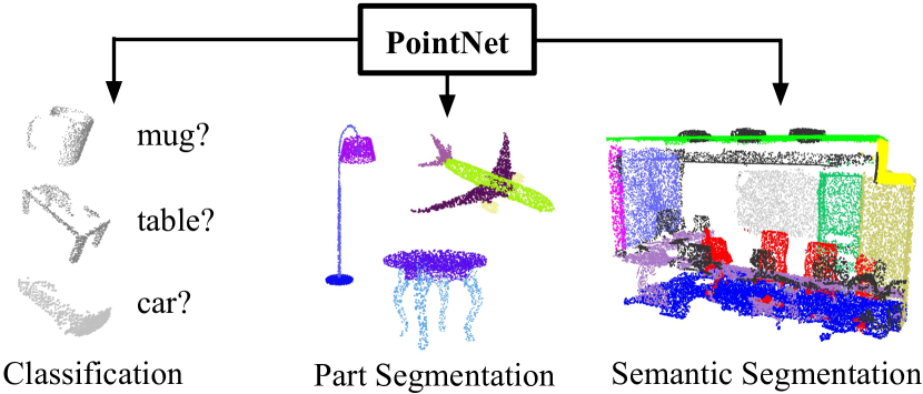
Our PointNet is a unified architecture that directly takes point clouds as input and outputs either class labels for the entire input or per point segment/part labels for each point of the input. The basic architecture of our network is surprisingly simple as in the initial stages each point is processed identically and independently. In the basic setting each point is represented by just its three coordinates . Additional dimensions may be added by computing normals and other local or global features.
Key to our approach is the use of a single symmetric function, max pooling. Effectively the network learns a set of optimization functions/criteria that select interesting or informative points of the point cloud and encode the reason for their selection. The final fully connected layers of the network aggregate these learnt optimal values into the global descriptor for the entire shape as mentioned above (shape classification) or are used to predict per point labels (shape segmentation).
Our input format is easy to apply rigid or affine transformations to, as each point transforms independently. Thus we can add a data-dependent spatial transformer network that attempts to canonicalize the data before the PointNet processes them, so as to further improve the results.
We provide both a theoretical analysis and an experimental evaluation of our approach. We show that our network can approximate any set function that is continuous. More interestingly, it turns out that our network learns to summarize an input point cloud by a sparse set of key points, which roughly corresponds to the skeleton of objects according to visualization. The theoretical analysis provides an understanding why our PointNet is highly robust to small perturbation of input points as well as to corruption through point insertion (outliers) or deletion (missing data).
On a number of benchmark datasets ranging from shape classification, part segmentation to scene segmentation, we experimentally compare our PointNet with state-of-the-art approaches based upon multi-view and volumetric representations. Under a unified architecture, not only is our PointNet much faster in speed, but it also exhibits strong performance on par or even better than state of the art.
The key contributions of our work are as follows:
-
•
We design a novel deep net architecture suitable for consuming unordered point sets in 3D;
-
•
We show how such a net can be trained to perform 3D shape classification, shape part segmentation and scene semantic parsing tasks;
-
•
We provide thorough empirical and theoretical analysis on the stability and efficiency of our method;
-
•
We illustrate the 3D features computed by the selected neurons in the net and develop intuitive explanations for its performance.
The problem of processing unordered sets by neural nets is a very general and fundamental problem – we expect that our ideas can be transferred to other domains as well.
2 Related Work
Point Cloud Features
Most existing features for point cloud are handcrafted towards specific tasks. Point features often encode certain statistical properties of points and are designed to be invariant to certain transformations, which are typically classified as intrinsic [2, 24, 3] or extrinsic [20, 19, 14, 10, 5]. They can also be categorized as local features and global features. For a specific task, it is not trivial to find the optimal feature combination.
Deep Learning on 3D Data
3D data has multiple popular representations, leading to various approaches for learning. Volumetric CNNs: [28, 17, 18] are the pioneers applying 3D convolutional neural networks on voxelized shapes. However, volumetric representation is constrained by its resolution due to data sparsity and computation cost of 3D convolution. FPNN [13] and Vote3D [26] proposed special methods to deal with the sparsity problem; however, their operations are still on sparse volumes, it’s challenging for them to process very large point clouds. Multiview CNNs: [23, 18] have tried to render 3D point cloud or shapes into 2D images and then apply 2D conv nets to classify them. With well engineered image CNNs, this line of methods have achieved dominating performance on shape classification and retrieval tasks [21]. However, it’s nontrivial to extend them to scene understanding or other 3D tasks such as point classification and shape completion. Spectral CNNs: Some latest works [4, 16] use spectral CNNs on meshes. However, these methods are currently constrained on manifold meshes such as organic objects and it’s not obvious how to extend them to non-isometric shapes such as furniture. Feature-based DNNs: [6, 8] firstly convert the 3D data into a vector, by extracting traditional shape features and then use a fully connected net to classify the shape. We think they are constrained by the representation power of the features extracted.
Deep Learning on Unordered Sets
From a data structure point of view, a point cloud is an unordered set of vectors. While most works in deep learning focus on regular input representations like sequences (in speech and language processing), images and volumes (video or 3D data), not much work has been done in deep learning on point sets.
One recent work from Oriol Vinyals et al [25] looks into this problem. They use a read-process-write network with attention mechanism to consume unordered input sets and show that their network has the ability to sort numbers. However, since their work focuses on generic sets and NLP applications, there lacks the role of geometry in the sets.
3 Problem Statement
We design a deep learning framework that directly consumes unordered point sets as inputs. A point cloud is represented as a set of 3D points , where each point is a vector of its coordinate plus extra feature channels such as color, normal etc. For simplicity and clarity, unless otherwise noted, we only use the coordinate as our point’s channels.
For the object classification task, the input point cloud is either directly sampled from a shape or pre-segmented from a scene point cloud. Our proposed deep network outputs scores for all the candidate classes. For semantic segmentation, the input can be a single object for part region segmentation, or a sub-volume from a 3D scene for object region segmentation. Our model will output scores for each of the points and each of the semantic sub-categories.
4 Deep Learning on Point Sets
4.1 Properties of Point Sets in
Our input is a subset of points from an Euclidean space. It has three main properties:
-
•
Unordered. Unlike pixel arrays in images or voxel arrays in volumetric grids, point cloud is a set of points without specific order. In other words, a network that consumes 3D point sets needs to be invariant to permutations of the input set in data feeding order.
-
•
Interaction among points. The points are from a space with a distance metric. It means that points are not isolated, and neighboring points form a meaningful subset. Therefore, the model needs to be able to capture local structures from nearby points, and the combinatorial interactions among local structures.
-
•
Invariance under transformations. As a geometric object, the learned representation of the point set should be invariant to certain transformations. For example, rotating and translating points all together should not modify the global point cloud category nor the segmentation of the points.
4.2 PointNet Architecture
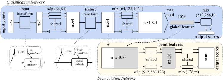
Our full network architecture is visualized in Fig 2, where the classification network and the segmentation network share a great portion of structures. Please read the caption of Fig 2 for the pipeline.
Our network has three key modules: the max pooling layer as a symmetric function to aggregate information from all the points, a local and global information combination structure, and two joint alignment networks that align both input points and point features.
We will discuss our reason behind these design choices in separate paragraphs below.
Symmetry Function for Unordered Input
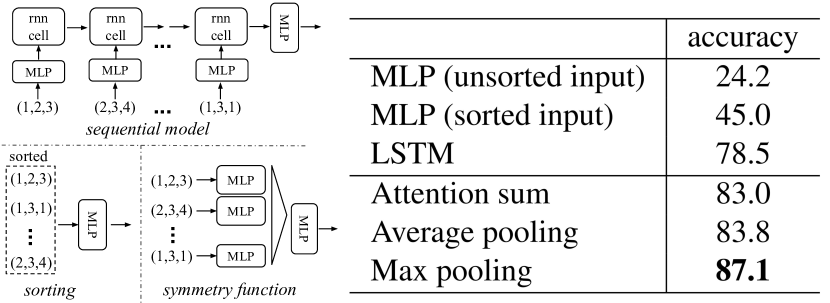
In order to make a model invariant to input permutation, three strategies exist: 1) sort input into a canonical order; 2) treat the input as a sequence to train an RNN, but augment the training data by all kinds of permutations; 3) use a simple symmetric function to aggregate the information from each point. Here, a symmetric function takes vectors as input and outputs a new vector that is invariant to the input order. For example, and operators are symmetric binary functions.
While sorting sounds like a simple solution, in high dimensional space there in fact does not exist an ordering that is stable w.r.t. point perturbations in the general sense. This can be easily shown by contradiction. If such an ordering strategy exists, it defines a bijection map between a high-dimensional space and a real line. It is not hard to see, to require an ordering to be stable w.r.t point perturbations is equivalent to requiring that this map preserves spatial proximity as the dimension reduces, a task that cannot be achieved in the general case. Therefore, sorting does not fully resolve the ordering issue, and it’s hard for a network to learn a consistent mapping from input to output as the ordering issue persists. As shown in experiments (Fig 5), we find that applying a MLP directly on the sorted point set performs poorly, though slightly better than directly processing an unsorted input.
The idea to use RNN considers the point set as a sequential signal and hopes that by training the RNN with randomly permuted sequences, the RNN will become invariant to input order. However in “OrderMatters” [25] the authors have shown that order does matter and cannot be totally omitted. While RNN has relatively good robustness to input ordering for sequences with small length (dozens), it’s hard to scale to thousands of input elements, which is the common size for point sets. Empirically, we have also shown that model based on RNN does not perform as well as our proposed method (Fig 5).
Our idea is to approximate a general function defined on a point set by applying a symmetric function on transformed elements in the set:
| (1) |
where , and is a symmetric function.
Empirically, our basic module is very simple: we approximate by a multi-layer perceptron network and by a composition of a single variable function and a max pooling function. This is found to work well by experiments. Through a collection of , we can learn a number of ’s to capture different properties of the set.
Local and Global Information Aggregation
The output from the above section forms a vector , which is a global signature of the input set. We can easily train a SVM or multi-layer perceptron classifier on the shape global features for classification. However, point segmentation requires a combination of local and global knowledge. We can achieve this by a simple yet highly effective manner.
Our solution can be seen in Fig 2 (Segmentation Network). After computing the global point cloud feature vector, we feed it back to per point features by concatenating the global feature with each of the point features. Then we extract new per point features based on the combined point features - this time the per point feature is aware of both the local and global information.
With this modification our network is able to predict per point quantities that rely on both local geometry and global semantics. For example we can accurately predict per-point normals (fig in supplementary), validating that the network is able to summarize information from the point’s local neighborhood. In experiment session, we also show that our model can achieve state-of-the-art performance on shape part segmentation and scene segmentation.
Joint Alignment Network
The semantic labeling of a point cloud has to be invariant if the point cloud undergoes certain geometric transformations, such as rigid transformation. We therefore expect that the learnt representation by our point set is invariant to these transformations.
A natural solution is to align all input set to a canonical space before feature extraction. Jaderberg et al. [9] introduces the idea of spatial transformer to align 2D images through sampling and interpolation, achieved by a specifically tailored layer implemented on GPU.
Our input form of point clouds allows us to achieve this goal in a much simpler way compared with [9]. We do not need to invent any new layers and no alias is introduced as in the image case. We predict an affine transformation matrix by a mini-network (T-net in Fig 2) and directly apply this transformation to the coordinates of input points. The mini-network itself resembles the big network and is composed by basic modules of point independent feature extraction, max pooling and fully connected layers. More details about the T-net are in the supplementary.
This idea can be further extended to the alignment of feature space, as well. We can insert another alignment network on point features and predict a feature transformation matrix to align features from different input point clouds. However, transformation matrix in the feature space has much higher dimension than the spatial transform matrix, which greatly increases the difficulty of optimization. We therefore add a regularization term to our softmax training loss. We constrain the feature transformation matrix to be close to orthogonal matrix:
| (2) |
where is the feature alignment matrix predicted by a mini-network. An orthogonal transformation will not lose information in the input, thus is desired. We find that by adding the regularization term, the optimization becomes more stable and our model achieves better performance.
4.3 Theoretical Analysis
Universal approximation
We first show the universal approximation ability of our neural network to continuous set functions. By the continuity of set functions, intuitively, a small perturbation to the input point set should not greatly change the function values, such as classification or segmentation scores.
Formally, let , is a continuous set function on w.r.t to Hausdorff distance , i.e., , for any , if , then . Our theorem says that can be arbitrarily approximated by our network given enough neurons at the max pooling layer, i.e., in (1) is sufficiently large.
Theorem 1.
Suppose is a continuous set function w.r.t Hausdorff distance . , a continuous function and a symmetric function , such that for any ,
where is the full list of elements in ordered arbitrarily, is a continuous function, and MAX is a vector max operator that takes vectors as input and returns a new vector of the element-wise maximum.
The proof to this theorem can be found in our supplementary material. The key idea is that in the worst case the network can learn to convert a point cloud into a volumetric representation, by partitioning the space into equal-sized voxels. In practice, however, the network learns a much smarter strategy to probe the space, as we shall see in point function visualizations.
Bottleneck dimension and stability
Theoretically and experimentally we find that the expressiveness of our network is strongly affected by the dimension of the max pooling layer, i.e., in (1). Here we provide an analysis, which also reveals properties related to the stability of our model.
We define to be the sub-network of which maps a point set in to a -dimensional vector. The following theorem tells us that small corruptions or extra noise points in the input set are not likely to change the output of our network:
Theorem 2.
Suppose such that and . Then,
-
(a)
, if ;
-
(b)
We explain the implications of the theorem. (a) says that is unchanged up to the input corruption if all points in are preserved; it is also unchanged with extra noise points up to . (b) says that only contains a bounded number of points, determined by in (1). In other words, is in fact totally determined by a finite subset of less or equal to elements. We therefore call the critical point set of and the bottleneck dimension of .
Combined with the continuity of , this explains the robustness of our model w.r.t point perturbation, corruption and extra noise points. The robustness is gained in analogy to the sparsity principle in machine learning models. Intuitively, our network learns to summarize a shape by a sparse set of key points. In experiment section we see that the key points form the skeleton of an object.
5 Experiment
| input | #views | accuracy | accuracy | |
| avg. class | overall | |||
| SPH [11] | mesh | - | 68.2 | - |
| 3DShapeNets [28] | volume | 1 | 77.3 | 84.7 |
| VoxNet [17] | volume | 12 | 83.0 | 85.9 |
| Subvolume [18] | volume | 20 | 86.0 | 89.2 |
| LFD [28] | image | 10 | 75.5 | - |
| MVCNN [23] | image | 80 | 90.1 | - |
| Ours baseline | point | - | 72.6 | 77.4 |
| Ours PointNet | point | 1 | 86.2 | 89.2 |
Experiments are divided into four parts. First, we show PointNets can be applied to multiple 3D recognition tasks (Sec 5.1). Second, we provide detailed experiments to validate our network design (Sec 5.2). At last we visualize what the network learns (Sec 5.3) and analyze time and space complexity (Sec 5.4).
| mean | aero | bag | cap | car | chair | ear | guitar | knife | lamp | laptop | motor | mug | pistol | rocket | skate | table | |
|---|---|---|---|---|---|---|---|---|---|---|---|---|---|---|---|---|---|
| phone | board | ||||||||||||||||
| # shapes | 2690 | 76 | 55 | 898 | 3758 | 69 | 787 | 392 | 1547 | 451 | 202 | 184 | 283 | 66 | 152 | 5271 | |
| Wu [27] | - | 63.2 | - | - | - | 73.5 | - | - | - | 74.4 | - | - | - | - | - | - | 74.8 |
| Yi [29] | 81.4 | 81.0 | 78.4 | 77.7 | 75.7 | 87.6 | 61.9 | 92.0 | 85.4 | 82.5 | 95.7 | 70.6 | 91.9 | 85.9 | 53.1 | 69.8 | 75.3 |
| 3DCNN | 79.4 | 75.1 | 72.8 | 73.3 | 70.0 | 87.2 | 63.5 | 88.4 | 79.6 | 74.4 | 93.9 | 58.7 | 91.8 | 76.4 | 51.2 | 65.3 | 77.1 |
| Ours | 83.7 | 83.4 | 78.7 | 82.5 | 74.9 | 89.6 | 73.0 | 91.5 | 85.9 | 80.8 | 95.3 | 65.2 | 93.0 | 81.2 | 57.9 | 72.8 | 80.6 |
5.1 Applications
In this section we show how our network can be trained to perform 3D object classification, object part segmentation and semantic scene segmentation 111More application examples such as correspondence and point cloud based CAD model retrieval are included in supplementary material.. Even though we are working on a brand new data representation (point sets), we are able to achieve comparable or even better performance on benchmarks for several tasks.
3D Object Classification
Our network learns global point cloud feature that can be used for object classification. We evaluate our model on the ModelNet40 [28] shape classification benchmark. There are 12,311 CAD models from 40 man-made object categories, split into 9,843 for training and 2,468 for testing. While previous methods focus on volumetric and mult-view image representations, we are the first to directly work on raw point cloud.
We uniformly sample 1024 points on mesh faces according to face area and normalize them into a unit sphere. During training we augment the point cloud on-the-fly by randomly rotating the object along the up-axis and jitter the position of each points by a Gaussian noise with zero mean and 0.02 standard deviation.
In Table 1, we compare our model with previous works as well as our baseline using MLP on traditional features extracted from point cloud (point density, D2, shape contour etc.). Our model achieved state-of-the-art performance among methods based on 3D input (volumetric and point cloud). With only fully connected layers and max pooling, our net gains a strong lead in inference speed and can be easily parallelized in CPU as well. There is still a small gap between our method and multi-view based method (MVCNN [23]), which we think is due to the loss of fine geometry details that can be captured by rendered images.
3D Object Part Segmentation
Part segmentation is a challenging fine-grained 3D recognition task. Given a 3D scan or a mesh model, the task is to assign part category label (e.g. chair leg, cup handle) to each point or face.
We evaluate on ShapeNet part data set from [29], which contains 16,881 shapes from 16 categories, annotated with 50 parts in total. Most object categories are labeled with two to five parts. Ground truth annotations are labeled on sampled points on the shapes.
We formulate part segmentation as a per-point classification problem. Evaluation metric is mIoU on points. For each shape S of category C, to calculate the shape’s mIoU: For each part type in category C, compute IoU between groundtruth and prediction. If the union of groundtruth and prediction points is empty, then count part IoU as 1. Then we average IoUs for all part types in category C to get mIoU for that shape. To calculate mIoU for the category, we take average of mIoUs for all shapes in that category.
In this section, we compare our segmentation version PointNet (a modified version of Fig 2, Segmentation Network) with two traditional methods [27] and [29] that both take advantage of point-wise geometry features and correspondences between shapes, as well as our own 3D CNN baseline. See supplementary for the detailed modifications and network architecture for the 3D CNN.
In Table 2, we report per-category and mean IoU(%) scores. We observe a 2.3% mean IoU improvement and our net beats the baseline methods in most categories.
| mean IoU | overall accuracy | |
|---|---|---|
| Ours baseline | 20.12 | 53.19 |
| Ours PointNet | 47.71 | 78.62 |
| table | chair | sofa | board | mean | |
|---|---|---|---|---|---|
| # instance | 455 | 1363 | 55 | 137 | |
| Armeni et al. [1] | 46.02 | 16.15 | 6.78 | 3.91 | 18.22 |
| Ours | 46.67 | 33.80 | 4.76 | 11.72 | 24.24 |
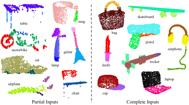
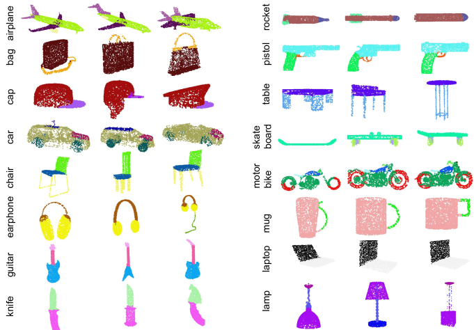
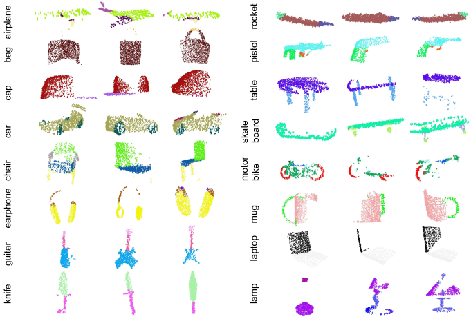
We also perform experiments on simulated Kinect scans to test the robustness of these methods. For every CAD model in the ShapeNet part data set, we use Blensor Kinect Simulator [7] to generate incomplete point clouds from six random viewpoints. We train our PointNet on the complete shapes and partial scans with the same network architecture and training setting. Results show that we lose only 5.3% mean IoU. In Fig 3, we present qualitative results on both complete and partial data. One can see that though partial data is fairly challenging, our predictions are reasonable.
Semantic Segmentation in Scenes
Our network on part segmentation can be easily extended to semantic scene segmentation, where point labels become semantic object classes instead of object part labels.
We experiment on the Stanford 3D semantic parsing data set [1]. The dataset contains 3D scans from Matterport scanners in 6 areas including 271 rooms. Each point in the scan is annotated with one of the semantic labels from 13 categories (chair, table, floor, wall etc. plus clutter).
To prepare training data, we firstly split points by room, and then sample rooms into blocks with area 1m by 1m. We train our segmentation version of PointNet to predict per point class in each block. Each point is represented by a 9-dim vector of XYZ, RGB and normalized location as to the room (from 0 to 1). At training time, we randomly sample 4096 points in each block on-the-fly. At test time, we test on all the points. We follow the same protocol as [1] to use k-fold strategy for train and test.
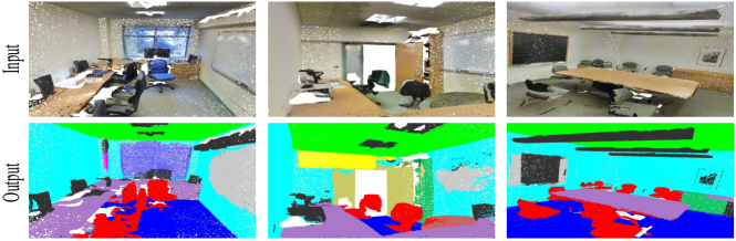
We compare our method with a baseline using handcrafted point features. The baseline extracts the same 9-dim local features and three additional ones: local point density, local curvature and normal. We use standard MLP as the classifier. Results are shown in Table 3, where our PointNet method significantly outperforms the baseline method. In Fig 4, we show qualitative segmentation results. Our network is able to output smooth predictions and is robust to missing points and occlusions.
Based on the semantic segmentation output from our network, we further build a 3D object detection system using connected component for object proposal (see supplementary for details). We compare with previous state-of-the-art method in Table 4. The previous method is based on a sliding shape method (with CRF post processing) with SVMs trained on local geometric features and global room context feature in voxel grids. Our method outperforms it by a large margin on the furniture categories reported.
5.2 Architecture Design Analysis
In this section we validate our design choices by control experiments. We also show the effects of our network’s hyperparameters.
Comparison with Alternative Order-invariant Methods
As mentioned in Sec 4.2, there are at least three options for consuming unordered set inputs. We use the ModelNet40 shape classification problem as a test bed for comparisons of those options, the following two control experiment will also use this task.
The baselines (illustrated in Fig 5) we compared with include multi-layer perceptron on unsorted and sorted points as arrays, RNN model that considers input point as a sequence, and a model based on symmetry functions. The symmetry operation we experimented include max pooling, average pooling and an attention based weighted sum. The attention method is similar to that in [25], where a scalar score is predicted from each point feature, then the score is normalized across points by computing a softmax. The weighted sum is then computed on the normalized scores and the point features. As shown in Fig 5, max-pooling operation achieves the best performance by a large winning margin, which validates our choice.
Effectiveness of Input and Feature Transformations
In Table 5 we demonstrate the positive effects of our input and feature transformations (for alignment). It’s interesting to see that the most basic architecture already achieves quite reasonable results. Using input transformation gives a performance boost. The regularization loss is necessary for the higher dimension transform to work. By combining both transformations and the regularization term, we achieve the best performance.
| Transform | accuracy |
|---|---|
| none | 87.1 |
| input (3x3) | 87.9 |
| feature (64x64) | 86.9 |
| feature (64x64) + reg. | 87.4 |
| both | 89.2 |
Robustness Test
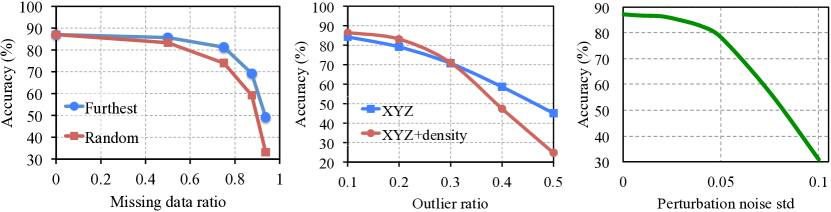
We show our PointNet, while simple and effective, is robust to various kinds of input corruptions. We use the same architecture as in Fig 5’s max pooling network. Input points are normalized into a unit sphere. Results are in Fig 6.
As to missing points, when there are points missing, the accuracy only drops by and w.r.t. furthest and random input sampling. Our net is also robust to outlier points, if it has seen those during training. We evaluate two models: one trained on points with coordinates; the other on plus point density. The net has more than accuracy even when of the points are outliers. Fig 6 right shows the net is robust to point perturbations.
5.3 Visualizing PointNet
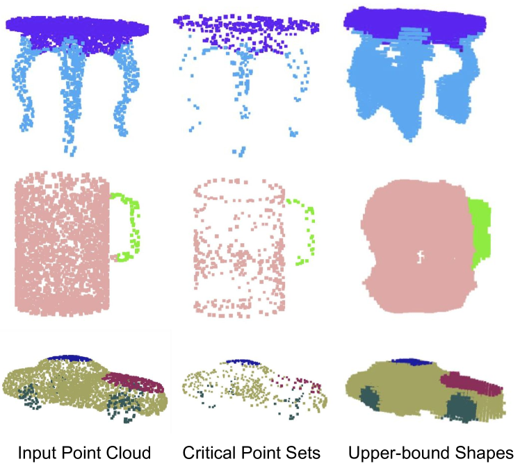
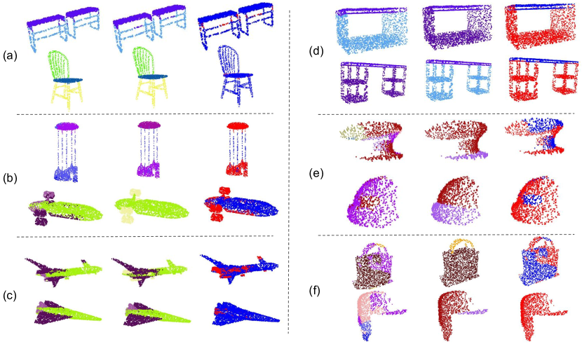
In Fig 7, we visualize critical point sets and upper-bound shapes (as discussed in Thm 2) for some sample shapes . The point sets between the two shapes will give exactly the same global shape feature .
We can see clearly from Fig 7 that the critical point sets , those contributed to the max pooled feature, summarizes the skeleton of the shape. The upper-bound shapes illustrates the largest possible point cloud that give the same global shape feature as the input point cloud . and reflect the robustness of PointNet, meaning that losing some non-critical points does not change the global shape signature at all.
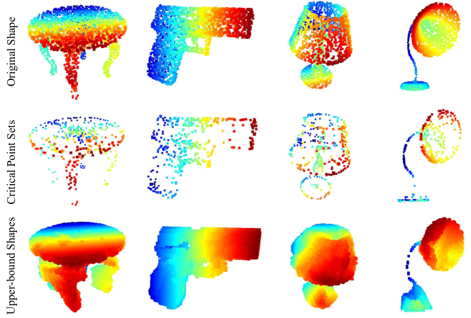
The is constructed by forwarding all the points in a edge-length-2 cube through the network and select points whose point function values are no larger than the global shape descriptor.
5.4 Time and Space Complexity Analysis
Table 6 summarizes space (number of parameters in the network) and time (floating-point operations/sample) complexity of our classification PointNet. We also compare PointNet to a representative set of volumetric and multi-view based architectures in previous works.
While MVCNN [23] and Subvolume (3D CNN) [18] achieve high performance, PointNet is orders more efficient in computational cost (measured in FLOPs/sample: 141x and 8x more efficient, respectively). Besides, PointNet is much more space efficient than MVCNN in terms of #param in the network (17x less parameters). Moreover, PointNet is much more scalable – it’s space and time complexity is – linear in the number of input points. However, since convolution dominates computing time, multi-view method’s time complexity grows squarely on image resolution and volumetric convolution based method grows cubically with the volume size.
Empirically, PointNet is able to process more than one million points per second for point cloud classification (around 1K objects/second) or semantic segmentation (around 2 rooms/second) with a 1080X GPU on TensorFlow, showing great potential for real-time applications.
| #params | FLOPs/sample | |
|---|---|---|
| PointNet (vanilla) | 0.8M | 148M |
| PointNet | 3.5M | 440M |
| Subvolume [18] | 16.6M | 3633M |
| MVCNN [23] | 60.0M | 62057M |
6 Conclusion
In this work, we propose a novel deep neural network PointNet that directly consumes point cloud. Our network provides a unified approach to a number of 3D recognition tasks including object classification, part segmentation and semantic segmentation, while obtaining on par or better results than state of the arts on standard benchmarks. We also provide theoretical analysis and visualizations towards understanding of our network.
Acknowledgement.
The authors gratefully acknowledge the support of a Samsung GRO grant, ONR MURI N00014-13-1-0341 grant, NSF grant IIS-1528025, a Google Focused Research Award, a gift from the Adobe corporation and hardware donations by NVIDIA.
References
- [1] I. Armeni, O. Sener, A. R. Zamir, H. Jiang, I. Brilakis, M. Fischer, and S. Savarese. 3d semantic parsing of large-scale indoor spaces. In Proceedings of the IEEE International Conference on Computer Vision and Pattern Recognition, 2016.
- [2] M. Aubry, U. Schlickewei, and D. Cremers. The wave kernel signature: A quantum mechanical approach to shape analysis. In Computer Vision Workshops (ICCV Workshops), 2011 IEEE International Conference on, pages 1626–1633. IEEE, 2011.
- [3] M. M. Bronstein and I. Kokkinos. Scale-invariant heat kernel signatures for non-rigid shape recognition. In Computer Vision and Pattern Recognition (CVPR), 2010 IEEE Conference on, pages 1704–1711. IEEE, 2010.
- [4] J. Bruna, W. Zaremba, A. Szlam, and Y. LeCun. Spectral networks and locally connected networks on graphs. arXiv preprint arXiv:1312.6203, 2013.
- [5] D.-Y. Chen, X.-P. Tian, Y.-T. Shen, and M. Ouhyoung. On visual similarity based 3d model retrieval. In Computer graphics forum, volume 22, pages 223–232. Wiley Online Library, 2003.
- [6] Y. Fang, J. Xie, G. Dai, M. Wang, F. Zhu, T. Xu, and E. Wong. 3d deep shape descriptor. In Proceedings of the IEEE Conference on Computer Vision and Pattern Recognition, pages 2319–2328, 2015.
- [7] M. Gschwandtner, R. Kwitt, A. Uhl, and W. Pree. BlenSor: Blender Sensor Simulation Toolbox Advances in Visual Computing. volume 6939 of Lecture Notes in Computer Science, chapter 20, pages 199–208. Springer Berlin / Heidelberg, Berlin, Heidelberg, 2011.
- [8] K. Guo, D. Zou, and X. Chen. 3d mesh labeling via deep convolutional neural networks. ACM Transactions on Graphics (TOG), 35(1):3, 2015.
- [9] M. Jaderberg, K. Simonyan, A. Zisserman, et al. Spatial transformer networks. In NIPS 2015.
- [10] A. E. Johnson and M. Hebert. Using spin images for efficient object recognition in cluttered 3d scenes. IEEE Transactions on pattern analysis and machine intelligence, 21(5):433–449, 1999.
- [11] M. Kazhdan, T. Funkhouser, and S. Rusinkiewicz. Rotation invariant spherical harmonic representation of 3 d shape descriptors. In Symposium on geometry processing, volume 6, pages 156–164, 2003.
- [12] Y. LeCun, L. Bottou, Y. Bengio, and P. Haffner. Gradient-based learning applied to document recognition. Proceedings of the IEEE, 86(11):2278–2324, 1998.
- [13] Y. Li, S. Pirk, H. Su, C. R. Qi, and L. J. Guibas. Fpnn: Field probing neural networks for 3d data. arXiv preprint arXiv:1605.06240, 2016.
- [14] H. Ling and D. W. Jacobs. Shape classification using the inner-distance. IEEE transactions on pattern analysis and machine intelligence, 29(2):286–299, 2007.
- [15] L. v. d. Maaten and G. Hinton. Visualizing data using t-sne. Journal of Machine Learning Research, 9(Nov):2579–2605, 2008.
- [16] J. Masci, D. Boscaini, M. Bronstein, and P. Vandergheynst. Geodesic convolutional neural networks on riemannian manifolds. In Proceedings of the IEEE International Conference on Computer Vision Workshops, pages 37–45, 2015.
- [17] D. Maturana and S. Scherer. Voxnet: A 3d convolutional neural network for real-time object recognition. In IEEE/RSJ International Conference on Intelligent Robots and Systems, September 2015.
- [18] C. R. Qi, H. Su, M. Nießner, A. Dai, M. Yan, and L. Guibas. Volumetric and multi-view cnns for object classification on 3d data. In Proc. Computer Vision and Pattern Recognition (CVPR), IEEE, 2016.
- [19] R. B. Rusu, N. Blodow, and M. Beetz. Fast point feature histograms (fpfh) for 3d registration. In Robotics and Automation, 2009. ICRA’09. IEEE International Conference on, pages 3212–3217. IEEE, 2009.
- [20] R. B. Rusu, N. Blodow, Z. C. Marton, and M. Beetz. Aligning point cloud views using persistent feature histograms. In 2008 IEEE/RSJ International Conference on Intelligent Robots and Systems, pages 3384–3391. IEEE, 2008.
- [21] M. Savva, F. Yu, H. Su, M. Aono, B. Chen, D. Cohen-Or, W. Deng, H. Su, S. Bai, X. Bai, et al. Shrec’16 track large-scale 3d shape retrieval from shapenet core55.
- [22] P. Y. Simard, D. Steinkraus, and J. C. Platt. Best practices for convolutional neural networks applied to visual document analysis. In ICDAR, volume 3, pages 958–962, 2003.
- [23] H. Su, S. Maji, E. Kalogerakis, and E. G. Learned-Miller. Multi-view convolutional neural networks for 3d shape recognition. In Proc. ICCV, to appear, 2015.
- [24] J. Sun, M. Ovsjanikov, and L. Guibas. A concise and provably informative multi-scale signature based on heat diffusion. In Computer graphics forum, volume 28, pages 1383–1392. Wiley Online Library, 2009.
- [25] O. Vinyals, S. Bengio, and M. Kudlur. Order matters: Sequence to sequence for sets. arXiv preprint arXiv:1511.06391, 2015.
- [26] D. Z. Wang and I. Posner. Voting for voting in online point cloud object detection. Proceedings of the Robotics: Science and Systems, Rome, Italy, 1317, 2015.
- [27] Z. Wu, R. Shou, Y. Wang, and X. Liu. Interactive shape co-segmentation via label propagation. Computers & Graphics, 38:248–254, 2014.
- [28] Z. Wu, S. Song, A. Khosla, F. Yu, L. Zhang, X. Tang, and J. Xiao. 3d shapenets: A deep representation for volumetric shapes. In Proceedings of the IEEE Conference on Computer Vision and Pattern Recognition, pages 1912–1920, 2015.
- [29] L. Yi, V. G. Kim, D. Ceylan, I.-C. Shen, M. Yan, H. Su, C. Lu, Q. Huang, A. Sheffer, and L. Guibas. A scalable active framework for region annotation in 3d shape collections. SIGGRAPH Asia, 2016.
Supplementary
Appendix A Overview
This document provides additional quantitative results, technical details and more qualitative test examples to the main paper.
In Sec B we extend the robustness test to compare PointNet with VoxNet on incomplete input. In Sec C we provide more details on neural network architectures, training parameters and in Sec D we describe our detection pipeline in scenes. Then Sec E illustrates more applications of PointNet, while Sec F shows more analysis experiments. Sec G provides a proof for our theory on PointNet. At last, we show more visualization results in Sec H.
Appendix B Comparison between PointNet and VoxNet (Sec 5.2)
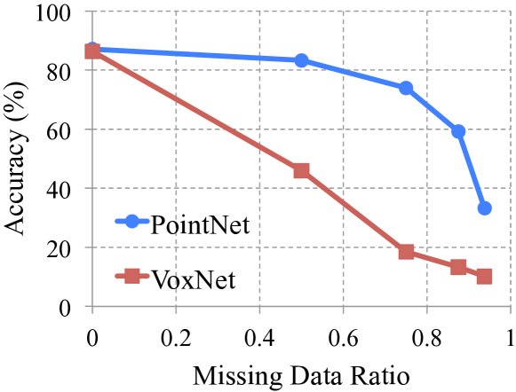
We extend the experiments in Sec 5.2 Robustness Test to compare PointNet and VoxNet [17] (a representative architecture for volumetric representation) on robustness to missing data in the input point cloud. Both networks are trained on the same train test split with 1024 number of points as input. For VoxNet we voxelize the point cloud to occupancy grids and augment the training data by random rotation around up-axis and jittering.
At test time, input points are randomly dropped out by a certain ratio. As VoxNet is sensitive to rotations, its prediction uses average scores from 12 viewpoints of a point cloud. As shown in Fig 8, we see that our PointNet is much more robust to missing points. VoxNet’s accuracy dramatically drops when half of the input points are missing, from to with a difference, while our PointNet only has a performance drop. This can be explained by the theoretical analysis and explanation of our PointNet – it is learning to use a collection of critical points to summarize the shape, thus it is very robust to missing data.
Appendix C Network Architecture and Training Details (Sec 5.1)
PointNet Classification Network
As the basic architecture is already illustrated in the main paper, here we provides more details on the joint alignment/transformation network and training parameters.
The first transformation network is a mini-PointNet that takes raw point cloud as input and regresses to a matrix. It’s composed of a shared network (with layer output sizes 64, 128, 1024) on each point, a max pooling across points and two fully connected layers with output sizes , . The output matrix is initialized as an identity matrix. All layers, except the last one, include ReLU and batch normalization. The second transformation network has the same architecture as the first one except that the output is a matrix. The matrix is also initialized as an identity. A regularization loss (with weight 0.001) is added to the softmax classification loss to make the matrix close to orthogonal.
We use dropout with keep ratio on the last fully connected layer, whose output dimension , before class score prediction. The decay rate for batch normalization starts with and is gradually increased to . We use adam optimizer with initial learning rate , momentum and batch size . The learning rate is divided by 2 every 20 epochs. Training on ModelNet takes 3-6 hours to converge with TensorFlow and a GTX1080 GPU.
PointNet Segmentation Network
The segmentation network is an extension to the classification PointNet. Local point features (the output after the second transformation network) and global feature (output of the max pooling) are concatenated for each point. No dropout is used for segmentation network. Training parameters are the same as the classification network.
As to the task of shape part segmentation, we made a few modifications to the basic segmentation network architecture (Fig 2 in main paper) in order to achieve best performance, as illustrated in Fig 9. We add a one-hot vector indicating the class of the input and concatenate it with the max pooling layer’s output. We also increase neurons in some layers and add skip links to collect local point features in different layers and concatenate them to form point feature input to the segmentation network.
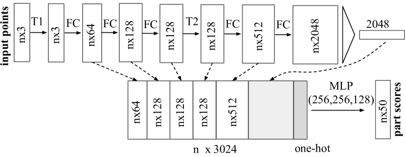
While [27] and [29] deal with each object category independently, due to the lack of training data for some categories (the total number of shapes for all the categories in the data set are shown in the first line), we train our PointNet across categories (but with one-hot vector input to indicate category). To allow fair comparison, when testing these two models, we only predict part labels for the given specific object category.
As to semantic segmentation task, we used the architecture as in Fig 2 in the main paper.
It takes around six to twelve hours to train the model on ShapeNet part dataset and around half a day to train on the Stanford semantic parsing dataset.
Baseline 3D CNN Segmentation Network
In ShapeNet part segmentation experiment, we compare our proposed segmentation version PointNet to two traditional methods as well as a 3D volumetric CNN network baseline. In Fig 10, we show the baseline 3D volumetric CNN network we use. We generalize the well-known 3D CNN architectures, such as VoxNet [17] and 3DShapeNets [28] to a fully convolutional 3D CNN segmentation network.
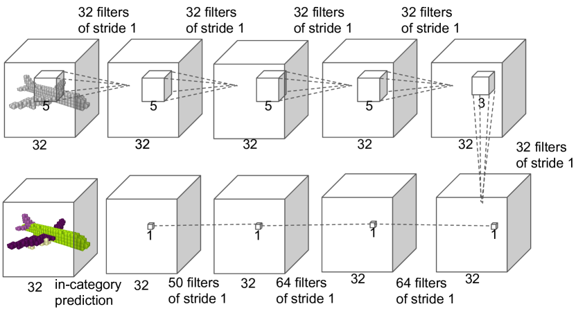
For a given point cloud, we first convert it to the volumetric representation as a occupancy grid with resolution . Then, five 3D convolution operations each with 32 output channels and stride of 1 are sequentially applied to extract features. The receptive field is 19 for each voxel. Finally, a sequence of 3D convolutional layers with kernel size is appended to the computed feature map to predict segmentation label for each voxel. ReLU and batch normalization are used for all layers except the last one. The network is trained across categories, however, in order to compare with other baseline methods where object category is given, we only consider output scores in the given object category.
Appendix D Details on Detection Pipeline (Sec 5.1)
We build a simple 3D object detection system based on the semantic segmentation results and our object classification PointNet.
We use connected component with segmentation scores to get object proposals in scenes. Starting from a random point in the scene, we find its predicted label and use BFS to search nearby points with the same label, with a search radius of meter. If the resulted cluster has more than 200 points (assuming a 4096 point sample in a 1m by 1m area), the cluster’s bounding box is marked as one object proposal. For each proposed object, it’s detection score is computed as the average point score for that category. Before evaluation, proposals with extremely small areas/volumes are pruned. For tables, chairs and sofas, the bounding boxes are extended to the floor in case the legs are separated with the seat/surface.
We observe that in some rooms such as auditoriums lots of objects (e.g. chairs) are close to each other, where connected component would fail to correctly segment out individual ones. Therefore we leverage our classification network and uses sliding shape method to alleviate the problem for the chair class. We train a binary classification network for each category and use the classifier for sliding window detection. The resulted boxes are pruned by non-maximum suppression. The proposed boxes from connected component and sliding shapes are combined for final evaluation.
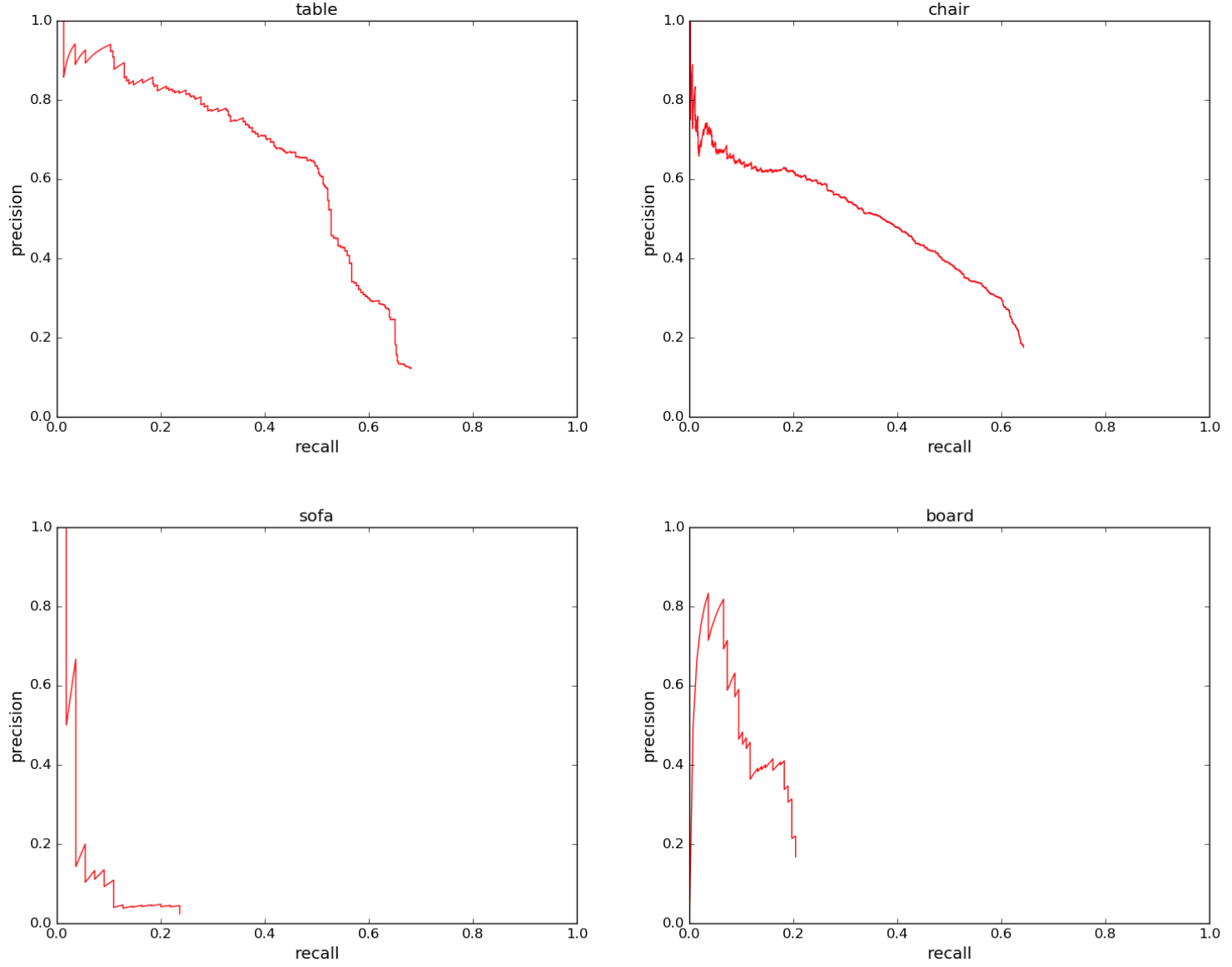
In Fig 11, we show the precision-recall curves for object detection. We trained six models, where each one of them is trained on five areas and tested on the left area. At test phase, each model is tested on the area it has never seen. The test results for all six areas are aggregated for the PR curve generation.
Appendix E More Applications (Sec 5.1)
Model Retrieval from Point Cloud
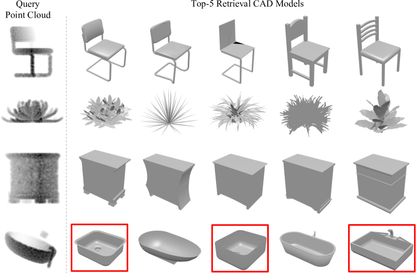
Our PointNet learns a global shape signature for every given input point cloud. We expect geometrically similar shapes have similar global signature. In this section, we test our conjecture on the shape retrieval application. To be more specific, for every given query shape from ModelNet test split, we compute its global signature (output of the layer before the score prediction layer) given by our classification PointNet and retrieve similar shapes in the train split by nearest neighbor search. Results are shown in Fig 12.
Shape Correspondence
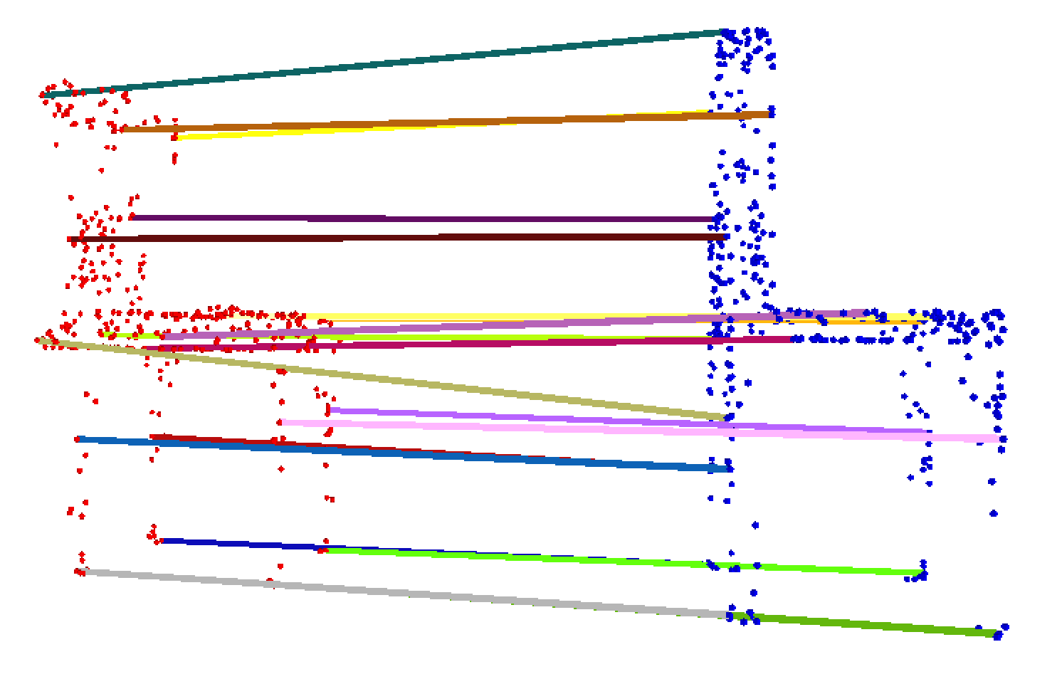
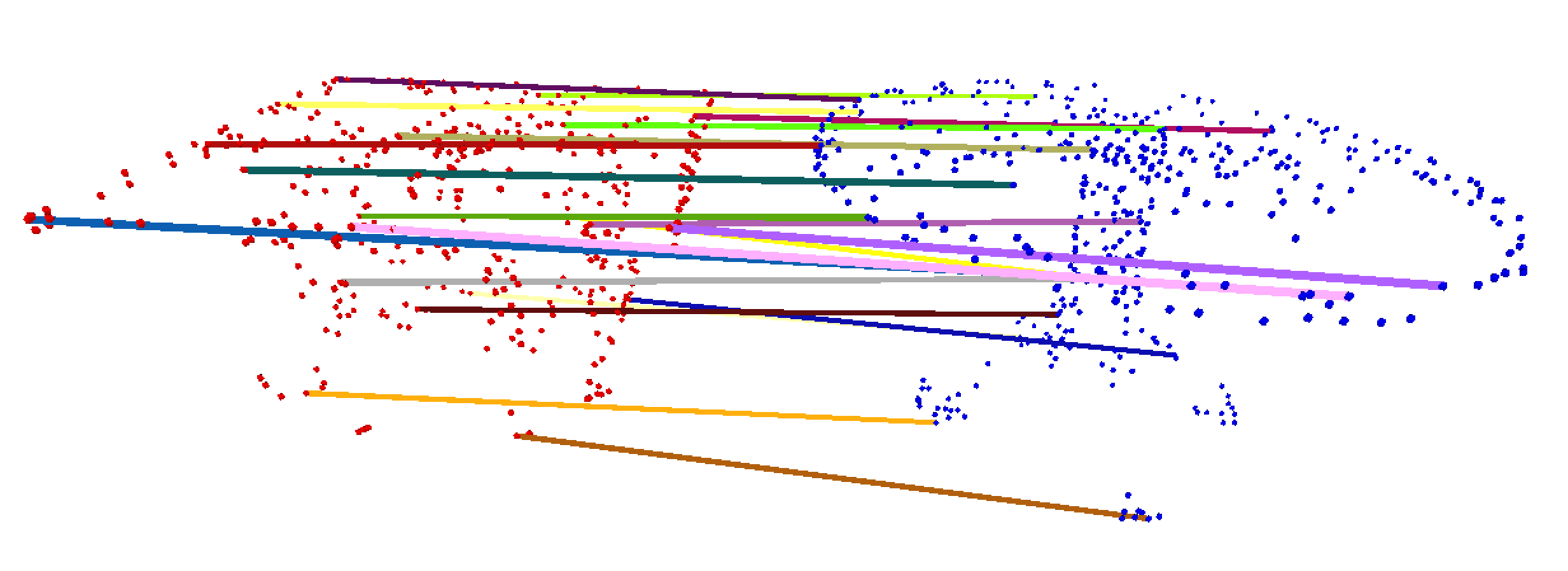
In this section, we show that point features learnt by PointNet can be potentially used to compute shape correspondences. Given two shapes, we compute the correspondence between their critical point sets ’s by matching the pairs of points that activate the same dimensions in the global features. Fig 13 and Fig 14 show the detected shape correspondence between two similar chairs and tables.
Appendix F More Architecture Analysis (Sec 5.2)
Effects of Bottleneck Dimension and Number of Input Points
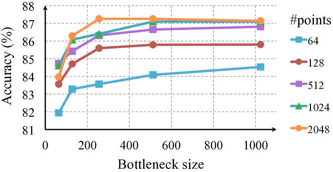
Here we show our model’s performance change with regard to the size of the first max layer output as well as the number of input points. In Fig 15 we see that performance grows as we increase the number of points however it saturates at around 1K points. The max layer size plays an important role, increasing the layer size from 64 to 1024 results in a performance gain. It indicates that we need enough point feature functions to cover the 3D space in order to discriminate different shapes.
It’s worth notice that even with 64 points as input (obtained from furthest point sampling on meshes), our network can achieve decent performance.
MNIST Digit Classification
While we focus on 3D point cloud learning, a sanity check experiment is to apply our network on a 2D point clouds - pixel sets.
To convert an MNIST image into a 2D point set we threshold pixel values and add the pixel (represented as a point with coordinate in the image) with values larger than 128 to the set. We use a set size of 256. If there are more than 256 pixels int he set, we randomly sub-sample it; if there are less, we pad the set with the one of the pixels in the set (due to our max operation, which point to use for the padding will not affect outcome).
As seen in Table 7, we compare with a few baselines including multi-layer perceptron that considers input image as an ordered vector, a RNN that consider input as sequence from pixel (0,0) to pixel (27,27), and a vanilla version CNN. While the best performing model on MNIST is still well engineered CNNs (achieving less than error rate), it’s interesting to see that our PointNet model can achieve reasonable performance by considering image as a 2D point set.
| input | error (%) | |
|---|---|---|
| Multi-layer perceptron [22] | vector | 1.60 |
| LeNet5 [12] | image | 0.80 |
| Ours PointNet | point set | 0.78 |
Normal Estimation
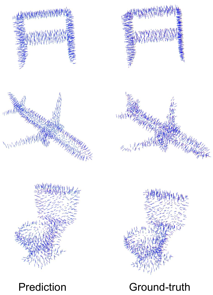
In segmentation version of PointNet, local point features and global feature are concatenated in order to provide context to local points. However, it’s unclear whether the context is learnt through this concatenation. In this experiment, we validate our design by showing that our segmentation network can be trained to predict point normals, a local geometric property that is determined by a point’s neighborhood.
We train a modified version of our segmentation PointNet in a supervised manner to regress to the ground-truth point normals. We just change the last layer of our segmentation PointNet to predict normal vector for each point. We use absolute value of cosine distance as loss.
Fig. 16 compares our PointNet normal prediction results (the left columns) to the ground-truth normals computed from the mesh (the right columns). We observe a reasonable normal reconstruction. Our predictions are more smooth and continuous than the ground-truth which includes flipped normal directions in some region.
Segmentation Robustness
As discussed in Sec 5.2 and Sec B, our PointNet is less sensitive to data corruption and missing points for classification tasks since the global shape feature is extracted from a collection of critical points from the given input point cloud. In this section, we show that the robustness holds for segmentation tasks too. The per-point part labels are predicted based on the combination of per-point features and the learnt global shape feature. In Fig 17, we illustrate the segmentation results for the given input point clouds (the left-most column), the critical point sets (the middle column) and the upper-bound shapes .
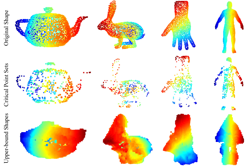
Network Generalizability to Unseen Shape Categories
In Fig 18, we visualize the critical point sets and the upper-bound shapes for new shapes from unseen categories (face, house, rabbit, teapot) that are not present in ModelNet or ShapeNet. It shows that the learnt per-point functions are generalizable. However, since we train mostly on man-made objects with lots of planar structures, the reconstructed upper-bound shape in novel categories also contain more planar surfaces.
Appendix G Proof of Theorem (Sec 4.3)
Let .
is a continuous function on w.r.t to Hausdorff distance if the following condition is satisfied:
, for any , if , then .
We show that can be approximated arbitrarily by composing a symmetric function and a continuous function.
Theorem 1.
Suppose is a continuous set function w.r.t Hausdorff distance . , a continuous function and a symmetric function , where is a continuous function, MAX is a vector max operator that takes vectors as input and returns a new vector of the element-wise maximum, such that for any ,
where are the elements of extracted in certain order,
Proof.
By the continuity of , we take so that for any .
Define , which split into intervals evenly and define an auxiliary function that maps a point to the left end of the interval it lies in:
Let , then
because .
Let be a soft indicator function where is the point to set (interval) distance. Let , then .
Let , indicating the occupancy of the -th interval by points in . Let , then is a symmetric function, indicating the occupancy of each interval by points in .
Define as , which maps the occupancy vector to a set which contains the left end of each occupied interval. It is easy to show:
where are the elements of extracted in certain order.
Let be a continuous function such that for . Then,
Note that can be rewritten as follows:
Obviously is a symmetric function. ∎
Next we give the proof of Theorem 2. We define to be the sub-network of which maps a point set in to a -dimensional vector. The following theorem tells us that small corruptions or extra noise points in the input set is not likely to change the output of our network:
Theorem 2.
Suppose such that and . Then,
-
(a)
, if ;
-
(b)
Proof.
Obviously, , is determined by . So we only need to prove that .
For the th dimension as the output of , there exists at least one such that , where is the th dimension of the output vector from . Take as the union of all for . Then, satisfies the above condition.
Adding any additional points such that at all dimensions to does not change , hence . Therefore, can be obtained adding the union of all such points to .
∎
Appendix H More Visualizations
Classification Visualization
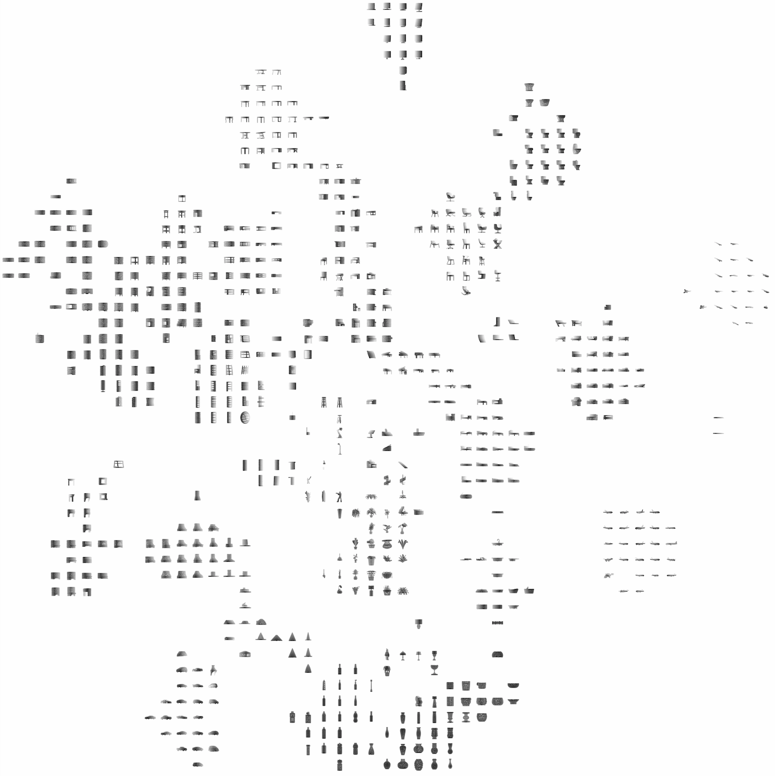
We use t-SNE[15] to embed point cloud global signature (1024-dim) from our classification PointNet into a 2D space. Fig 20 shows the embedding space of ModelNet 40 test split shapes. Similar shapes are clustered together according to their semantic categories.
Segmentation Visualization
We present more segmentation results on both complete CAD models and simulated Kinect partial scans. We also visualize failure cases with error analysis. Fig 21 and Fig 22 show more segmentation results generated on complete CAD models and their simulated Kinect scans. Fig 23 illustrates some failure cases. Please read the caption for the error analysis.
Scene Semantic Parsing Visualization
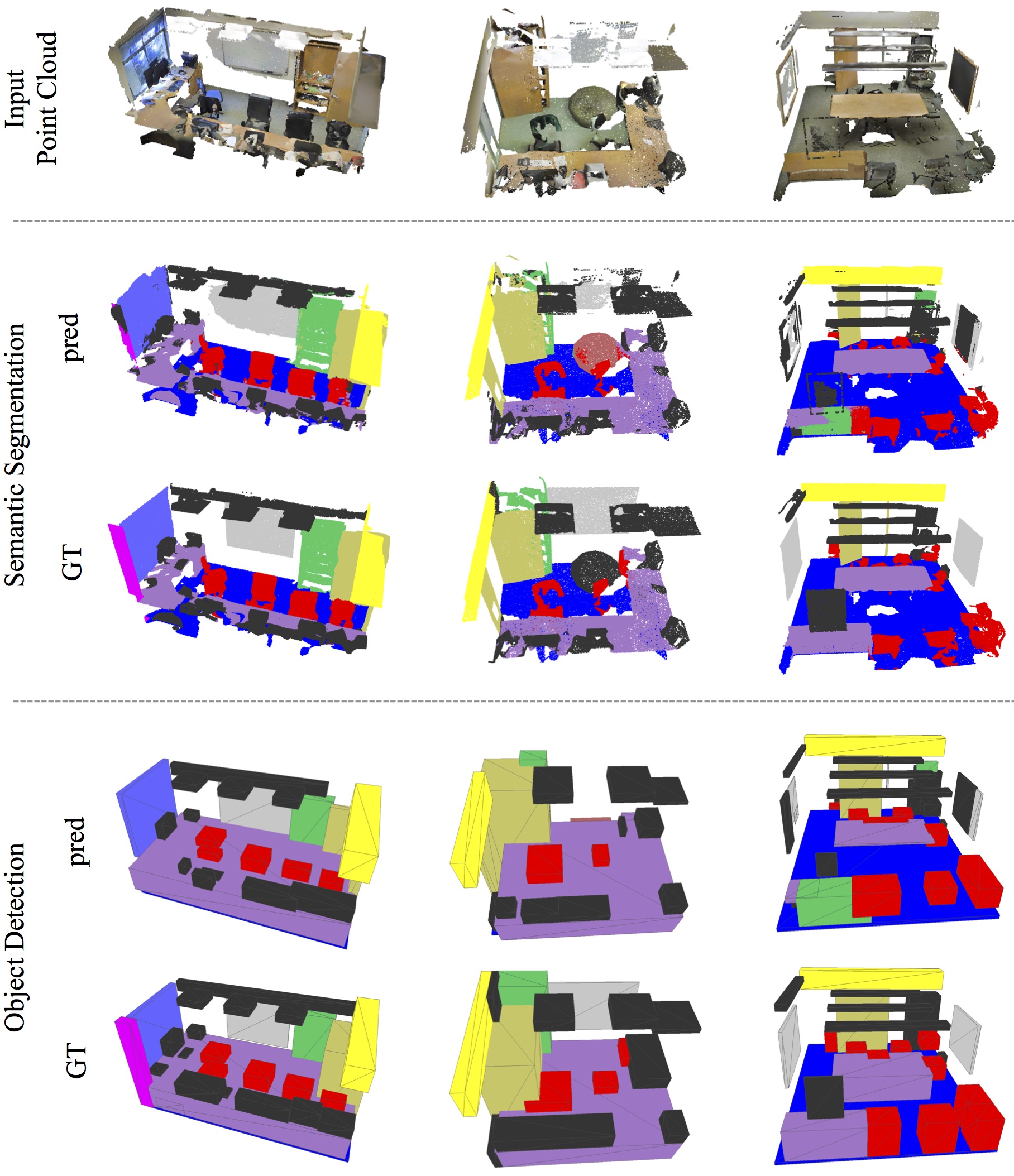
We give a visualization of semantic parsing in Fig 24 where we show input point cloud, prediction and ground truth for both semantic segmentation and object detection for two office rooms and one conference room. The area and the rooms are unseen in the training set.
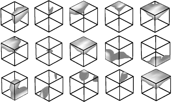
Point Function Visualization
Our classification PointNet computes (we take in this visualization) dimension point features for each point and aggregates all the per-point local features via a max pooling layer into a single -dim vector, which forms the global shape descriptor.
To gain more insights on what the learnt per-point functions ’s detect, we visualize the points ’s that give high per-point function value in Fig 19. This visualization clearly shows that different point functions learn to detect for points in different regions with various shapes scattered in the whole space.