A Calculus of Cyber-Physical Systems

Abstract

We propose a hybrid process calculus for modelling and reasoning on cyber-physical systems (CPSs). The dynamics of the calculus is expressed in terms of a labelled transition system in the SOS style of Plotkin. This is used to define a bisimulation-based behavioural semantics which support compositional reasonings. Finally, we prove run-time properties and system equalities for a non-trivial case study.

1 Introduction

Cyber-Physical Systems (CPSs) are integrations of networking and distributed computing systems with physical processes, where feedback loops allow physical processes to affect computations and vice versa. For example, in real-time control systems, a hierarchy of sensors, actuators and control processing components are connected to control stations. Different kinds of CPSs include supervisory control and data acquisition (SCADA), programmable logic controllers (PLC) and distributed control systems.

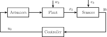
Figure 1: Structure of a CPS

The physical plant of a CPS is typically represented by means of a discrete-time state-space model consisting of two equations of the form

$\begin{array}[]{rcl}x_{k+1}&=&Ax_{k}+Bu_{k}+w_{k}\\[2.0pt] y_{k}&=&Cx_{k}+e_{k}\end{array}$

where $x_{k}\in\mathbb{R}^{n}$ is the current (physical) state, $u_{k}\in\mathbb{R}^{m}$ is the input (i.e., the control actions implemented through actuators) and $y_{k}\in\mathbb{R}^{p}$ is the output (i.e., the measurements from the sensors). The uncertainty $w_{k}\in\mathbb{R}^{n}$ and the measurement error $e_{k}\in\mathbb{R}^{p}$ represent perturbation and sensor noise, respectively, and $A$, $B$, and $C$ are matrices modelling the dynamics of the physical system. The next state $x_{k+1}$ depends on the current state $x_{k}$ and the corresponding control actions $u_{k}$, at the sampling instant $k\in\mathbb{N}$. Note that, the state $x_{k}$ cannot be directly observed: only its measurements $y_{k}$ can be observed.

The physical plant is supported by a communication network through which the sensor measurements and actuator data are exchanged with the controller(s), i.e., the cyber component, also called logics, of a CPS (see Figure 1).

The range of CPSs applications is rapidly increasing and already covers several domains [10]: advanced automotive systems, energy conservation, environmental monitoring, avionics, critical infrastructure control (electric power, water resources, and communications systems for example), etc.

However, there is still a lack of research on the modelling and validation of CPSs through formal methodologies that might allow to model the interactions among the system components, and to verify the correctness of a CPS, as a whole, before its practical implementation. A straightforward utilisation of these techniques is for model-checking, i.e. to statically assess whether the current system deployment can guarantee the expected behaviour. However, they can also be an important aid for system planning, for instance to decide whether different deployments for a given application are behavioural equivalent.

In this paper, we propose a contribution in the area of formal methods for CPSs, by defining a hybrid process calculus, called CCPS, with a clearly-defined behavioural semantics for specifying and reasoning on CPSs. In CCPS, systems are represented as terms of the form $E\,{\Join}\,P$, where $E$ denotes the physical plant (also called environment) of the system, containing information on state variables, actuators, sensors, evolution law, etc., while $P$ represents the cyber component of the system, i.e., the controller that governs sensor reading and actuator writing, as well as channel-based communication with other cyber components. Thus, channels are used for logical interactions between cyber components, whereas sensors and actuators make possible the interaction between cyber and physical components. Despite this conceptual similarity, messages transmitted via channels are “consumed” upon reception, whereas actuators’ states (think of a valve) remains unchanged until its controller modifies it.

CCPS is equipped with a labelled transition semantics (LTS) in the SOS style of Plotkin [19]. We prove that our labelled transition semantics satisfies some standard time properties such as: time determinism, patience, maximal progress, and well-timedness. Based on our LTS, we define a natural notion of weak bisimilarity. As a main result, we prove that our bisimilarity is a congruence and it is hence suitable for compositional reasoning. We are not aware of similar results in the context of CPSs. Finally, we provide a non-trivial case study, taken from an engineering application, and use it to illustrate our definitions and our semantic theory for CPSs. Here, we wish to remark that while we have kept the example simple, it is actually far from trivial and designed to show that various CPSs can be modelled in this style.

Outline

In § 2, we give syntax and operational semantics of CCPS. In § 3 we provide a bisimulation-based behavioural semantics for CCPS and prove its compositionality. In § 4 we model in CCPS our case study, and prove for it run-time properties as well as system equalities. In § 5, we discuss related and future work.

2 The Calculus

In this section, we introduce our Calculus of Cyber-Physical Systems CCPS. Let us start with some preliminary notations. We use $x,x_{k}\in\cal X$ for state variables; $c,d\in\cal C$ for communication channels, $a,a_{k}\in\cal A$ for actuator devices, $s,s_{k}\in\cal S$ for sensors devices. Actuator names are metavariables for actuator devices like $\mathit{valve}$, $\mathit{light}$, etc. Similarly, sensor names are metavariables for sensor devices, e.g., a sensor $\mathit{thermometer}$ that measures, with a given precision, a state variable called $\mathit{temperature}$. Values, ranged over by $v,v^{\prime}\in\cal V$, are built from basic values, such as Booleans, integers and real numbers; they also include names.

Given a generic set of names $\cal N$, we write $\mathbb{R}^{\cal N}$ to denote the set of functions assigning a real value to each name in $\cal N$. For $\xi\in\mathbb{R}^{\cal N}$, $n\in\cal N$ and $v\in\mathbb{R}$, we write $\xi[n\mapsto v]$ to denote the function $\psi\in\mathbb{R}^{\cal N}$ such that $\psi(m)=\xi(m)$, for any $m\neq n$, and $\psi(n)=v$. For $\xi,\xi^{\prime}\in\mathbb{R}^{\cal N}$, we write $\xi\leq\xi^{\prime}$ if $\xi(x)\leq\xi^{\prime}(x)$, for any $x\in{\cal N}$. Given $\xi_{1}\in\mathbb{R}^{{\cal N}_{1}}$ and $\xi_{2}\in\mathbb{R}^{{\cal N}_{2}}$ such that ${{\cal N}_{1}}\cap{{\cal N}_{2}}=\emptyset$, we denote with $\xi_{1}\uplus\xi_{2}$ the function in $\mathbb{R}^{{\cal N}_{1}\cup{\cal N}_{2}}$ such that $(\xi_{1}\uplus\xi_{2})(x)=\xi_{1}(x)$, if $x\in{{\cal N}_{1}}$, and $(\xi_{1}\uplus\xi_{2})(x)=\xi_{2}(x)$, if $x\in{{\cal N}_{2}}$. Finally, given $\xi\in\mathbb{R}^{{\cal N}}$ and a set of names ${\cal M}\subseteq{\cal N}$, we write $\xi\raise-2.15277pt\hbox{$|$}_{\cal M}$ for the restriction of function $\xi$ to the set ${{\cal M}}$.

In CCPS, a cyber-physical system consists of two components: a physical environment $E$ that encloses all physical aspects of a system (state variables, physical devices, evolution law, etc) and a cyber component, represented as a concurrent process $P$ that interacts with the physical devices (sensors and actuators) of the system, and can communicate, via channels, with other processes of the same CPS or with processes of other CPSs.

We write $E\,{\Join}\,P$ to denote the resulting CPS, and use $M$ and $N$ to range over CPSs. Let us formally define physical environments.

Definition 1 (Physical environment)

Let $\hat{\mathcal{X}}\subseteq\mathcal{X}$ be a set of state variables, $\hat{\mathcal{A}}\subseteq\mathcal{A}$ be a set of actuators, and $\hat{\mathcal{S}}\subseteq\mathcal{S}$ be a set of sensors. A physical environment $E$ is 7-tuple $\langle\xi_{\mathrm{x}}{},\xi_{\mathrm{u}}{},\xi_{\mathrm{w}}{},\mathit{evol}{},\xi_{\mathrm{e}}{},\mathit{meas}{},\mathit{inv}{}\rangle$, where:

• $\xi_{\mathrm{x}}{}\in\mathbb{R}^{\hat{\cal X}}$ is the state function,

• $\xi_{\mathrm{u}}{}\in\mathbb{R}^{\hat{\cal A}}$ is the actuator function,

• $\xi_{\mathrm{w}}{}\in\mathbb{R}^{\hat{\cal X}}$ is the uncertainty function,

• $\mathit{evol}{}:\mathbb{R}^{\hat{\cal X}}\times\mathbb{R}^{\hat{\cal A}}\times\mathbb{R}^{\hat{\cal X}}\rightarrow 2^{\mathbb{R}^{\hat{\cal X}}}$ is the evolution map,

• $\xi_{\mathrm{e}}{}\in\mathbb{R}^{\hat{\cal S}}$ is the sensor-error function,

• $\mathit{meas}{}:\mathbb{R}^{\hat{\cal X}}\times\mathbb{R}^{\hat{\cal S}}\rightarrow 2^{\mathbb{R}^{\hat{\cal S}}}$ is the measurement map,

• $\mathit{inv}{}:\mathbb{R}^{\hat{\cal X}}\rightarrow\{\mathsf{true},\mathsf{false}\}$ is the invariant function.

All the functions defining an environment are total functions.

The state function $\xi_{\mathrm{x}}{}$ returns the current value (in $\mathbb{R}$) associated to each state variable of the system. The actuator function $\xi_{\mathrm{u}}{}$ returns the current value associated to each actuator. The uncertainty function $\xi_{\mathrm{w}}{}$ returns the uncertainty associated to each state variable. Thus, given a state variable $x\in\hat{\cal X}$, $\xi_{\mathrm{w}}{}(x)$ returns the maximum distance between the real value of $x$ and its representation in the model. Both the state function and the actuator function are supposed to change during the evolution of the system, whereas the uncertainty function is supposed to be constant.

Given a state function, an actuator function, and an uncertainty function, the evolution map $\mathit{evol}{}$ returns the set of next admissible state functions. This function models the evolution law of the physical system, where changes made on actuators may reflect on state variables. Since we assume an uncertainty in our models, the evolution map does not return a single state function but a set of possible state functions. The evolution map is obviously monotone with respect to uncertainty: if $\xi_{\mathrm{w}}{}\leq\xi_{\mathrm{w}}^{\prime}{}$ then $\mathit{evol}{}(\xi_{\mathrm{x}}{},\xi_{\mathrm{u}}{},\xi_{\mathrm{w}}{})\subseteq\mathit{evol}{}(\xi_{\mathrm{x}}{},\xi_{\mathrm{u}}{},\xi_{\mathrm{w}}^{\prime}{})$. Note also that, although the uncertainty function is constant, it can be used in the evolution map in an arbitrary way (e.g., it could have a heavier weight when a state variable reaches extreme values).

The sensor-error function $\xi_{\mathrm{e}}{}$ returns the maximum error associated to each sensor in $\hat{\cal S}$. Again due to the presence of the sensor-error function, the measurement map $\mathit{meas}{}$, given the current state function, returns a set of admissible measurement functions rather than a single one.

Finally, the invariant function $\mathit{inv}{}$ represents the conditions that the state variables must satisfy to allow for the evolution of the system. A CPS whose state variables don’t satisfy the invariant is in deadlock.

Let us now formalise in CCPS the cyber components of CPSs. Our (logical) processes build on the timed process algebra TPL [9] (basically CCS enriched with a discrete notion of time). We extend TPL with two constructs: one to read values detected at sensors, and one to write values on actuators. The remaining processes of the calculus are the same as those of TPL.

Definition 2 (Processes)

Processes are defined by the grammar:
$\begin{array}[]{rl}P,Q\>\;::=&\mathsf{nil}\>\;\,\big{|}\>\;\mathsf{idle}.P\>\;\big{|}\>\;P\parallel Q\>\;\big{|}\>\;\lfloor\pi.P\rfloor Q\>\;\big{|}\>\;[b]\{P\},\{Q\}\>\;\big{|}\>\;P{\setminus}c\>\;\big{|}\>\;X\>\;\big{|}\>\;{\mathsf{rec}}\,X.P\,.\end{array}$

We write $\mathsf{nil}$ for the terminated process. The process $\mathsf{idle}.P$ sleeps for one time unit and then continues as $P$. We write $P\parallel Q$ to denote the parallel composition of concurrent processes $P$ and $Q$. The process $\lfloor\pi.P\rfloor Q$, with $\pi\in\{\mathsf{snd}\,c\langle{v}\rangle,\mathsf{rcv}\,c({x}),\mathsf{read}\,s(x),\mathsf{write}\,a\langle v\rangle\}$, denotes prefixing with timeout. Thus, $\lfloor\mathsf{snd}\,c\langle{v}\rangle.P\rfloor Q$ sends the value $v$ on channel $c$ and, after that, it continues as $P$; otherwise, if no communication partner is available within one time unit, it evolves into $Q$. The process $\lfloor\mathsf{rcv}\,c({x}).P\rfloor Q$ is the obvious counterpart for receiving. $\lfloor\mathsf{read}\,s(x).P\rfloor Q$ reads the value $v$ detected by the sensor $s$ and, after that, it continues as $P$, where $x$ is replaced by $v$; otherwise, after one time unit, it evolves into $Q$. $\lfloor\mathsf{write}\,a\langle v\rangle.P\rfloor Q$ writes the value $v$ on the actuator $a$ and, after that, it continues as $P$; otherwise, after one time unit, it evolves into $Q$. The process $P{\setminus}c$ is the channel restriction operator of CCS. It is quantified over the set $\cal C$ of communication channels but we often use the shorthand $P{\setminus}C$ to mean $P{\setminus}{c_{1}}{\setminus}{c_{2}}\cdots{\setminus}{c_{n}}$, for $C=\{c_{1},c_{2},\ldots,c_{n}\}$. The process $[b]\{P\},\{Q\}$ is the standard conditional, where $b$ is a decidable guard. For simiplicity, as in CCS, we identify process $[b]\{P\},\{Q\}$ with $P$, if $b$ evaluates to true, and $[b]\{P\},\{Q\}$ with $Q$, if $b$ evaluates to false. In processes of the form $\mathsf{idle}.Q$ and $\lfloor\pi.P\rfloor Q$, the occurrence of $Q$ is said to be time-guarded. The process ${\mathsf{rec}}\,X.P$ denotes time-guarded recursion as all occurrences of the process variable $X$ may only occur time-guarded in $P$.

In the two constructs $\lfloor\mathsf{rcv}\,c({x}).P\rfloor Q$ and $\lfloor\mathsf{read}\,s(x).P\rfloor Q$, the variable $x$ is said to be bound. Similarly, the process variable $X$ is bound in ${\mathsf{rec}}\,X.P$. This gives rise to the standard notions of free/bound (process) variables and $\alpha$-conversion. We identify processes up to $\alpha$-conversion (similarly, we identify CPSs up to renaming of state variables, sensor names, and actuator names). A term is closed if it does not contain free (process) variables, and we assume to always work with closed processes: the absence of free variables is preserved at run-time. As further notation, we write $T{\{^{v}\!/\!_{x}\}}$ for the substitution of the variable $x$ with the value $v$ in any expression $T$ of our language. Similarly, $T{\{^{P}\!/\!_{X}\}}$ is the substitution of the process variable $X$ with the process $P$ in $T$.

The syntax of our CPSs is slightly too permissive as a process might use sensors and/or actuators which are not defined in the physical environment.

Definition 3 (Well-formedness)

Given a process $P$ and an environment $E=\langle\xi_{\mathrm{x}}{},\xi_{\mathrm{u}}{},\xi_{\mathrm{w}}{},\mathit{evol}{},\xi_{\mathrm{e}}{},\mathit{meas}{},\mathit{inv}{}\rangle$, the CPS $E\,{\Join}\,P$ is well-formed if: (i) for any sensor $s$ mentioned in $P$, the function $\xi_{\mathrm{e}}{}$ is defined in $s$; (ii) for any actuator $a$ mentioned in $P$, the function $\xi_{\mathrm{u}}{}$ is defined in $a$.

Hereafter, we will always work with well-formed networks.

Finally, we assume a number of notational conventions. We write $\pi.P$ instead of ${\mathsf{rec}}\,X.\lfloor\pi.P\rfloor X$, when $X$ does not occur in $P$. We write $\mathsf{snd}\,c$ (resp. $\mathsf{rcv}\,c$) when channel $c$ is used for pure synchronisation. For $k\geq 0$, we write $\mathsf{idle}^{k}.P$ as a shorthand for $\mathsf{idle}.\mathsf{idle}.\ldots\mathsf{idle}.P$, where the prefix $\mathsf{idle}$ appears $k$ consecutive times. Given $M=E\,{\Join}\,P$, we write $M\parallel Q$ for $E\,{\Join}\,(P\parallel Q)$, and $M{\setminus}c$ for $E\,{\Join}\,P{\setminus}c$.

2.1 Labelled Transition Semantics

In this section, we provide the dynamics of CCPS in terms of a labelled transition system (LTS) in the SOS style of Plotkin. In Definition 4, for convenience, we define some auxiliary operators on environments.

Definition 4

Let $E=\langle\xi_{\mathrm{x}}{},\xi_{\mathrm{u}}{},\xi_{\mathrm{w}}{},\mathit{evol}{},\xi_{\mathrm{e}}{},\mathit{meas}{},\mathit{inv}{}\rangle$.

• $\mathit{read\_sensor}(E,s)=\{\xi(s):\xi\in\mathit{meas}{}(\xi_{\mathrm{x}}{},\xi_{\mathrm{e}}{})\}$,

• $\mathit{update\_act}(E,a,v)=\langle\xi_{\mathrm{x}}{},\xi_{\mathrm{u}}{}[a{\mapsto}v],\xi_{\mathrm{w}}{},\mathit{evol}{},\xi_{\mathrm{e}}{},\mathit{meas}{},\allowbreak\mathit{inv}{}\rangle$,

• $\mathit{next}(E)=\bigcup_{\xi\in\mathit{evol}{}(\xi_{\mathrm{x}}{},\xi_{\mathrm{u}}{},\xi_{\mathrm{w}}{})}\{\langle\xi,\xi_{\mathrm{u}}{},\xi_{\mathrm{w}}{},\mathit{evol}{},\xi_{\mathrm{e}}{},\mathit{meas}{},\mathit{inv}{}\rangle\}$,

• $\mathit{inv}{}(E)=\mathit{inv}{}(\xi_{\mathrm{x}}{})$.

The operator $\mathit{read\_sensor}(E,s)$ returns the set of possible measurements detected by sensor $s$ in the environment $E$; it returns a set of possible values rather than a single value due to the error $\xi_{\mathrm{e}}{}(s)$ of sensor $s$. $\mathit{update\_act}(E,a,v)$ returns the new environment in which the actuator function is updated in such a manner to associate the actuator $a$ with the value $v$. $\mathit{next}(E)$ returns the set of the next admissible environments reachable from $E$, by an application of the evolution map. $\mathit{inv}{}(E)$ checks whether the state variables satisfy the invariant (here, with an abuse of notation, we overload the meaning of the function $\mathit{inv}{}$).

$$\begin{array}[]{l@{\hspace*{3mm}}l}{\mbox{\small(Outp)}}\>\;\begin{array}[]{c}-\\[2.0pt] \hline\cr{\lfloor\mathsf{snd}\,c\langle{v}\rangle.P\rfloor Q}\mathrel{\;\raisebox{0.0pt}{$\stackrel{{\scriptstyle\,\overline{c}v}}{{\makebox[16.31091pt]{\rule{0.0pt}{4.30554pt}\mbox{}\leavevmode\xleaders\hbox{$\mkern-2.6mu\relbar\mkern-2.6mu$}\hfill\mbox{}}}}$}\rightarrow}P\end{array}\hfil\hskip 8.53581pt&{\mbox{\small(Inpp)}}\>\;\begin{array}[]{c}-\\[2.0pt] \hline\cr{\lfloor\mathsf{rcv}\,c({x}).P\rfloor Q}\mathrel{\;\raisebox{0.0pt}{$\stackrel{{\scriptstyle\,cv}}{{\makebox[14.34018pt]{\rule{0.0pt}{4.30554pt}\mbox{}\leavevmode\xleaders\hbox{$\mkern-2.6mu\relbar\mkern-2.6mu$}\hfill\mbox{}}}}$}\rightarrow}{P{\{^{v}\!/\!_{x}\}}}\end{array}\par\\[14.0pt] {\mbox{\small(Write)}}\>\;\begin{array}[]{c}-\\[2.0pt] \hline\cr{\lfloor\mathsf{write}\,a\langle v\rangle.P\rfloor Q}\mathrel{\;\raisebox{0.0pt}{$\stackrel{{\scriptstyle\,a!v}}{{\makebox[16.95546pt]{\rule{0.0pt}{4.30554pt}\mbox{}\leavevmode\xleaders\hbox{$\mkern-2.6mu\relbar\mkern-2.6mu$}\hfill\mbox{}}}}$}\rightarrow}P\end{array}\hfil\hskip 8.53581pt&{\mbox{\small(Read)}}\>\;\begin{array}[]{c}-\\[2.0pt] \hline\cr{\lfloor\mathsf{read}\,s(x).P\rfloor Q}\mathrel{\;\raisebox{0.0pt}{$\stackrel{{\scriptstyle\,s?v}}{{\makebox[17.8977pt]{\rule{0.0pt}{4.30554pt}\mbox{}\leavevmode\xleaders\hbox{$\mkern-2.6mu\relbar\mkern-2.6mu$}\hfill\mbox{}}}}$}\rightarrow}{P{\{^{v}\!/\!_{x}\}}}\end{array}\\[14.0pt] {\mbox{\small(Com)}}\>\;\begin{array}[]{c}P\mathrel{\;\raisebox{0.0pt}{$\stackrel{{\scriptstyle\,\overline{c}v}}{{\makebox[16.31091pt]{\rule{0.0pt}{4.30554pt}\mbox{}\leavevmode\xleaders\hbox{$\mkern-2.6mu\relbar\mkern-2.6mu$}\hfill\mbox{}}}}$}\rightarrow}{P^{\prime}}\quad Q\mathrel{\;\raisebox{0.0pt}{$\stackrel{{\scriptstyle\,cv}}{{\makebox[14.34018pt]{\rule{0.0pt}{4.30554pt}\mbox{}\leavevmode\xleaders\hbox{$\mkern-2.6mu\relbar\mkern-2.6mu$}\hfill\mbox{}}}}$}\rightarrow}{Q^{\prime}}\\[2.0pt] \hline\cr P\parallel Q\mathrel{\;\raisebox{0.0pt}{$\stackrel{{\scriptstyle\,\tau}}{{\makebox[10.72676pt]{\rule{0.0pt}{4.30554pt}\mbox{}\leavevmode\xleaders\hbox{$\mkern-2.6mu\relbar\mkern-2.6mu$}\hfill\mbox{}}}}$}\rightarrow}{P^{\prime}\parallel Q^{\prime}}\end{array}\hfil\hskip 8.53581pt&{\mbox{\small(Par)}}\>\;\begin{array}[]{c}P\mathrel{\;\raisebox{0.0pt}{$\stackrel{{\scriptstyle\,\lambda}}{{\makebox[11.75003pt]{\rule{0.0pt}{4.30554pt}\mbox{}\leavevmode\xleaders\hbox{$\mkern-2.6mu\relbar\mkern-2.6mu$}\hfill\mbox{}}}}$}\rightarrow}P^{\prime}\quad\lambda\neq\mathsf{idle}\\[2.0pt] \hline\cr{P\parallel Q}\mathrel{\;\raisebox{0.0pt}{$\stackrel{{\scriptstyle\,\lambda}}{{\makebox[11.75003pt]{\rule{0.0pt}{4.30554pt}\mbox{}\leavevmode\xleaders\hbox{$\mkern-2.6mu\relbar\mkern-2.6mu$}\hfill\mbox{}}}}$}\rightarrow}{P^{\prime}\parallel Q}\end{array}\\[14.0pt] {\mbox{\small(ChnRes)}}\>\;\begin{array}[]{c}P\mathrel{\;\raisebox{0.0pt}{$\stackrel{{\scriptstyle\,\lambda}}{{\makebox[11.75003pt]{\rule{0.0pt}{4.30554pt}\mbox{}\leavevmode\xleaders\hbox{$\mkern-2.6mu\relbar\mkern-2.6mu$}\hfill\mbox{}}}}$}\rightarrow}P^{\prime}\quad\lambda\not\in\{{cv},{\overline{c}v}\}\\[2.0pt] \hline\cr P{\setminus}c\mathrel{\;\raisebox{0.0pt}{$\stackrel{{\scriptstyle\,\lambda}}{{\makebox[11.75003pt]{\rule{0.0pt}{4.30554pt}\mbox{}\leavevmode\xleaders\hbox{$\mkern-2.6mu\relbar\mkern-2.6mu$}\hfill\mbox{}}}}$}\rightarrow}{P^{\prime}}{\setminus}c\end{array}\hfil\hskip 8.53581pt&{\mbox{\small(Rec)}}\>\;\begin{array}[]{c}{P{\{^{{\mathsf{rec}}\,X.P}\!/\!_{X}\}}}\mathrel{\;\raisebox{0.0pt}{$\stackrel{{\scriptstyle\,\lambda}}{{\makebox[11.75003pt]{\rule{0.0pt}{4.30554pt}\mbox{}\leavevmode\xleaders\hbox{$\mkern-2.6mu\relbar\mkern-2.6mu$}\hfill\mbox{}}}}$}\rightarrow}Q\\[2.0pt] \hline\cr{{\mathsf{rec}}\,X.P}\mathrel{\;\raisebox{0.0pt}{$\stackrel{{\scriptstyle\,\lambda}}{{\makebox[11.75003pt]{\rule{0.0pt}{4.30554pt}\mbox{}\leavevmode\xleaders\hbox{$\mkern-2.6mu\relbar\mkern-2.6mu$}\hfill\mbox{}}}}$}\rightarrow}Q\end{array}\\[14.0pt] {\mbox{\small(TimeNil)}}\>\;\begin{array}[]{c}-\\[2.0pt] \hline\cr\mathsf{nil}\mathrel{\;\raisebox{0.0pt}{$\stackrel{{\scriptstyle\,\mathsf{idle}}}{{\makebox[18.55559pt]{\rule{0.0pt}{4.30554pt}\mbox{}\leavevmode\xleaders\hbox{$\mkern-2.6mu\relbar\mkern-2.6mu$}\hfill\mbox{}}}}$}\rightarrow}\mathsf{nil}\end{array}\hfil\hskip 8.53581pt&{\mbox{\small(Delay)}}\>\;\begin{array}[]{c}-\\[2.0pt] \hline\cr{\mathsf{idle}.P}\mathrel{\;\raisebox{0.0pt}{$\stackrel{{\scriptstyle\,\mathsf{idle}}}{{\makebox[18.55559pt]{\rule{0.0pt}{4.30554pt}\mbox{}\leavevmode\xleaders\hbox{$\mkern-2.6mu\relbar\mkern-2.6mu$}\hfill\mbox{}}}}$}\rightarrow}P\end{array}\\[14.0pt] {\mbox{\small(Timeout)}}\>\;\begin{array}[]{c}-\\[2.0pt] \hline\cr{\lfloor\pi.P\rfloor Q}\mathrel{\;\raisebox{0.0pt}{$\stackrel{{\scriptstyle\,\mathsf{idle}}}{{\makebox[18.55559pt]{\rule{0.0pt}{4.30554pt}\mbox{}\leavevmode\xleaders\hbox{$\mkern-2.6mu\relbar\mkern-2.6mu$}\hfill\mbox{}}}}$}\rightarrow}Q\end{array}\hfil\hskip 8.53581pt&{\mbox{\small(TimePar)}}\>\;\begin{array}[]{c}P\mathrel{\;\raisebox{0.0pt}{$\stackrel{{\scriptstyle\,\mathsf{idle}}}{{\makebox[18.55559pt]{\rule{0.0pt}{4.30554pt}\mbox{}\leavevmode\xleaders\hbox{$\mkern-2.6mu\relbar\mkern-2.6mu$}\hfill\mbox{}}}}$}\rightarrow}{P^{\prime}}\>\;\,Q\mathrel{\;\raisebox{0.0pt}{$\stackrel{{\scriptstyle\,\mathsf{idle}}}{{\makebox[18.55559pt]{\rule{0.0pt}{4.30554pt}\mbox{}\leavevmode\xleaders\hbox{$\mkern-2.6mu\relbar\mkern-2.6mu$}\hfill\mbox{}}}}$}\rightarrow}{Q^{\prime}}\>\;\,P\parallel Q\not\!\!\!\mathrel{\;\raisebox{0.0pt}{$\stackrel{{\scriptstyle\,\tau}}{{\makebox[10.72676pt]{\rule{0.0pt}{4.30554pt}\mbox{}\leavevmode\xleaders\hbox{$\mkern-2.6mu\relbar\mkern-2.6mu$}\hfill\mbox{}}}}$}\rightarrow}\\[2.0pt] \hline\cr{P\parallel Q}\mathrel{\;\raisebox{0.0pt}{$\stackrel{{\scriptstyle\,\mathsf{idle}}}{{\makebox[18.55559pt]{\rule{0.0pt}{4.30554pt}\mbox{}\leavevmode\xleaders\hbox{$\mkern-2.6mu\relbar\mkern-2.6mu$}\hfill\mbox{}}}}$}\rightarrow}{P^{\prime}\parallel Q^{\prime}}\end{array}\end{array}$$

Table 1: LTS for processes

$$\begin{array}[]{c}{\mbox{\small(Out)}}\>\;\begin{array}[]{c}P\mathrel{\;\raisebox{0.0pt}{$\stackrel{{\scriptstyle\,\overline{c}v}}{{\makebox[16.31091pt]{\rule{0.0pt}{4.30554pt}\mbox{}\leavevmode\xleaders\hbox{$\mkern-2.6mu\relbar\mkern-2.6mu$}\hfill\mbox{}}}}$}\rightarrow}P^{\prime}\quad\mathit{inv}{}(E)\\[2.0pt] \hline\cr E\,{\Join}\,P\mathrel{\;\raisebox{0.0pt}{$\stackrel{{\scriptstyle\,\overline{c}v}}{{\makebox[16.31091pt]{\rule{0.0pt}{4.30554pt}\mbox{}\leavevmode\xleaders\hbox{$\mkern-2.6mu\relbar\mkern-2.6mu$}\hfill\mbox{}}}}$}\rightarrow}E\,{\Join}\,P^{\prime}\end{array}\quad\quad\quad\quad{\mbox{\small(Inp)}}\>\;\begin{array}[]{c}P\mathrel{\;\raisebox{0.0pt}{$\stackrel{{\scriptstyle\,cv}}{{\makebox[14.34018pt]{\rule{0.0pt}{4.30554pt}\mbox{}\leavevmode\xleaders\hbox{$\mkern-2.6mu\relbar\mkern-2.6mu$}\hfill\mbox{}}}}$}\rightarrow}P^{\prime}\quad\mathit{inv}{}(E)\\[2.0pt] \hline\cr E\,{\Join}\,P\mathrel{\;\raisebox{0.0pt}{$\stackrel{{\scriptstyle\,cv}}{{\makebox[14.34018pt]{\rule{0.0pt}{4.30554pt}\mbox{}\leavevmode\xleaders\hbox{$\mkern-2.6mu\relbar\mkern-2.6mu$}\hfill\mbox{}}}}$}\rightarrow}E\,{\Join}\,P^{\prime}\end{array}\\[16.0pt] {\mbox{\small(SensRead)}}\>\;\begin{array}[]{c}P\mathrel{\;\raisebox{0.0pt}{$\stackrel{{\scriptstyle\,s?v}}{{\makebox[17.8977pt]{\rule{0.0pt}{4.30554pt}\mbox{}\leavevmode\xleaders\hbox{$\mkern-2.6mu\relbar\mkern-2.6mu$}\hfill\mbox{}}}}$}\rightarrow}P^{\prime}\quad\mathit{inv}{}(E)\quad\mbox{\small{$v\in\mathit{read\_sensor}(E,s)$}}\\[2.0pt] \hline\cr E\,{\Join}\,P\mathrel{\;\raisebox{0.0pt}{$\stackrel{{\scriptstyle\,\tau}}{{\makebox[10.72676pt]{\rule{0.0pt}{4.30554pt}\mbox{}\leavevmode\xleaders\hbox{$\mkern-2.6mu\relbar\mkern-2.6mu$}\hfill\mbox{}}}}$}\rightarrow}E\,{\Join}\,P^{\prime}\end{array}\\[16.0pt] {\mbox{\small(ActWrite)}}\>\;\begin{array}[]{c}P\mathrel{\;\raisebox{0.0pt}{$\stackrel{{\scriptstyle\,a!v}}{{\makebox[16.95546pt]{\rule{0.0pt}{4.30554pt}\mbox{}\leavevmode\xleaders\hbox{$\mkern-2.6mu\relbar\mkern-2.6mu$}\hfill\mbox{}}}}$}\rightarrow}{P^{\prime}}\quad\mathit{inv}{}(E)\quad{E^{\prime}}=\mathit{update\_act}(E,a,v)\\[2.0pt] \hline\cr E\,{\Join}\,P\mathrel{\;\raisebox{0.0pt}{$\stackrel{{\scriptstyle\,\tau}}{{\makebox[10.72676pt]{\rule{0.0pt}{4.30554pt}\mbox{}\leavevmode\xleaders\hbox{$\mkern-2.6mu\relbar\mkern-2.6mu$}\hfill\mbox{}}}}$}\rightarrow}E^{\prime}\,{\Join}\,P^{\prime}\end{array}\\[16.0pt] {\mbox{\small(Tau)}}\>\;\begin{array}[]{c}P\mathrel{\;\raisebox{0.0pt}{$\stackrel{{\scriptstyle\,\tau}}{{\makebox[10.72676pt]{\rule{0.0pt}{4.30554pt}\mbox{}\leavevmode\xleaders\hbox{$\mkern-2.6mu\relbar\mkern-2.6mu$}\hfill\mbox{}}}}$}\rightarrow}P^{\prime}\quad\mathit{inv}{}(E)\\[2.0pt] \hline\cr E\,{\Join}\,P\mathrel{\;\raisebox{0.0pt}{$\stackrel{{\scriptstyle\,\tau}}{{\makebox[10.72676pt]{\rule{0.0pt}{4.30554pt}\mbox{}\leavevmode\xleaders\hbox{$\mkern-2.6mu\relbar\mkern-2.6mu$}\hfill\mbox{}}}}$}\rightarrow}E\,{\Join}\,P^{\prime}\end{array}\quad\;{\mbox{\small(Time)}}\>\;\begin{array}[]{c}P\mathrel{\;\raisebox{0.0pt}{$\stackrel{{\scriptstyle\,\mathsf{idle}}}{{\makebox[18.55559pt]{\rule{0.0pt}{4.30554pt}\mbox{}\leavevmode\xleaders\hbox{$\mkern-2.6mu\relbar\mkern-2.6mu$}\hfill\mbox{}}}}$}\rightarrow}{P^{\prime}}\>\;\;E\,{\Join}\,P\mathrel{{\mathrel{\;\raisebox{0.0pt}{$\stackrel{{\scriptstyle\,\tau}}{{\makebox[10.72676pt]{\rule{0.0pt}{4.30554pt}\mbox{}\leavevmode\xleaders\hbox{$\mkern-2.6mu\relbar\mkern-2.6mu$}\hfill\mbox{}}}}$}\rightarrow}}\makebox[0.0pt][r]{$\not$\hskip 8.61108pt}}{\!}\>\;\;\mathit{inv}{}(E)\>\;\;E^{\prime}\in\mathit{next}(E)\\[2.0pt] \hline\cr E\,{\Join}\,P\mathrel{\;\raisebox{0.0pt}{$\stackrel{{\scriptstyle\,\mathsf{idle}}}{{\makebox[18.55559pt]{\rule{0.0pt}{4.30554pt}\mbox{}\leavevmode\xleaders\hbox{$\mkern-2.6mu\relbar\mkern-2.6mu$}\hfill\mbox{}}}}$}\rightarrow}E^{\prime}\,{\Join}\,P^{\prime}\end{array}\end{array}$$

Table 2: LTS for CPSs

In Table 1, we provide transition rules for processes. Here, the meta-variable $\lambda$ ranges over labels in the set $\{\mathsf{idle},\tau,{\overline{c}v},{cv},\allowbreak a!v,s?v\}$. Rules (Outp), (Inpp) and (Com) serve to model channel communication, on some channel $c$. Rules (Write) denotes the writing of some data $v$ on an actuator $a$. Rule (Read) denotes the reading of some data $v$ via a sensor $s$. Rule (Par) propagates untimed actions over parallel components. Rules (ChnRes) and (Rec) are the standard rules for channel restriction and recursion, respectively. The following four rules are standard, and model the passage of one time unit. The symmetric counterparts of rules (Com) and (Par) are obvious and thus omitted from the table.
In Table 2, we lift the transition rules from processes to systems. All rules have a common premise $\mathit{inv}{}(E)$: a CPS can evolve only if the invariant is satisfied, otherwise it is deadlocked. Here, actions, ranged over by $\alpha$, are in the set $\{\tau,{\overline{c}v},{cv},\mathsf{idle}\}$. These actions denote: non-observable activities ($\tau$); observable logical activities, i.e., channel transmission (${\overline{c}v}$ and ${cv}$); the passage of time ($\mathsf{idle}$). Rules (Out) and (Inp) model transmission and reception, with an external system, on a channel $c$. Rule (SensRead) models the reading of the current data detected at sensor $s$. Rule (ActWrite) models the writing of a value $v$ on an actuator $a$. Rule (Tau) lifts non-observable actions from processes to systems. A similar lifting occurs in rule (Time) for timed actions, where $\mathit{next}(E)$ returns the set of possible environments for the next time slot. Thus, by an application of rule (Time) a CPS moves to the next physical state, in the next time slot.
Now, having defined the actions that can be performed by a CPS, we can easily concatenate these actions to define execution traces. Formally, given a trace $t=\alpha_{1}\ldots\alpha_{n}$, we will write $\mathrel{\;\raisebox{0.0pt}{$\stackrel{{\scriptstyle\,t}}{{\makebox[10.19447pt]{\rule{0.0pt}{4.30554pt}\mbox{}\leavevmode\xleaders\hbox{$\mkern-2.6mu\relbar\mkern-2.6mu$}\hfill\mbox{}}}}$}\rightarrow}$ as an abbreviation for $\mathrel{\;\raisebox{0.0pt}{$\stackrel{{\scriptstyle\,\alpha_{1}}}{{\makebox[14.14459pt]{\rule{0.0pt}{4.30554pt}\mbox{}\leavevmode\xleaders\hbox{$\mkern-2.6mu\relbar\mkern-2.6mu$}\hfill\mbox{}}}}$}\rightarrow}\ldots\mathrel{\;\raisebox{0.0pt}{$\stackrel{{\scriptstyle\,\alpha_{n}}}{{\makebox[14.54553pt]{\rule{0.0pt}{4.30554pt}\mbox{}\leavevmode\xleaders\hbox{$\mkern-2.6mu\relbar\mkern-2.6mu$}\hfill\mbox{}}}}$}\rightarrow}$.
Below, we report a few desirable time properties which hold in our calculus: (a) time determinism, (b) maximal progress, (c) patience, and (d) well-timedness (symbol $\equiv$ denotes standard structural congruence for timed processes [17, 15]).

Theorem 2.1 (Time properties)

Let $M=E\,{\Join}\,P$.

• If $M\mathrel{\;\raisebox{0.0pt}{$\stackrel{{\scriptstyle\,\mathsf{idle}}}{{\makebox[18.55559pt]{\rule{0.0pt}{4.30554pt}\mbox{}\leavevmode\xleaders\hbox{$\mkern-2.6mu\relbar\mkern-2.6mu$}\hfill\mbox{}}}}$}\rightarrow}\hat{E}\,{\Join}\,Q$ and $M\mathrel{\;\raisebox{0.0pt}{$\stackrel{{\scriptstyle\,\mathsf{idle}}}{{\makebox[18.55559pt]{\rule{0.0pt}{4.30554pt}\mbox{}\leavevmode\xleaders\hbox{$\mkern-2.6mu\relbar\mkern-2.6mu$}\hfill\mbox{}}}}$}\rightarrow}\tilde{E}\,{\Join}\,R$, then $\{\hat{E},\tilde{E}\}\subseteq\mathit{next}{(E)}$ and $Q\equiv R$.

• If $M\mathrel{\;\raisebox{0.0pt}{$\stackrel{{\scriptstyle\,\tau}}{{\makebox[10.72676pt]{\rule{0.0pt}{4.30554pt}\mbox{}\leavevmode\xleaders\hbox{$\mkern-2.6mu\relbar\mkern-2.6mu$}\hfill\mbox{}}}}$}\rightarrow}M^{\prime}$ then there is no $M^{\prime\prime}$ such that $M\mathrel{\;\raisebox{0.0pt}{$\stackrel{{\scriptstyle\,\mathsf{idle}}}{{\makebox[18.55559pt]{\rule{0.0pt}{4.30554pt}\mbox{}\leavevmode\xleaders\hbox{$\mkern-2.6mu\relbar\mkern-2.6mu$}\hfill\mbox{}}}}$}\rightarrow}M^{\prime\prime}$.

• If $M\mathrel{\;\raisebox{0.0pt}{$\stackrel{{\scriptstyle\,\mathsf{idle}}}{{\makebox[18.55559pt]{\rule{0.0pt}{4.30554pt}\mbox{}\leavevmode\xleaders\hbox{$\mkern-2.6mu\relbar\mkern-2.6mu$}\hfill\mbox{}}}}$}\rightarrow}M^{\prime}$ for no $M^{\prime}$ then either $\mathit{next}(E)=\emptyset$ or $\mathit{inv}{(M)}=\mathsf{false}$ or there is $N$ such that $M\mathrel{\;\raisebox{0.0pt}{$\stackrel{{\scriptstyle\,\tau}}{{\makebox[10.72676pt]{\rule{0.0pt}{4.30554pt}\mbox{}\leavevmode\xleaders\hbox{$\mkern-2.6mu\relbar\mkern-2.6mu$}\hfill\mbox{}}}}$}\rightarrow}N$.

• For any $M$ there is a $k\in\mathbb{N}$ such that if $M\mathrel{\;\raisebox{0.0pt}{$\stackrel{{\scriptstyle\,\alpha_{1}}}{{\makebox[14.14459pt]{\rule{0.0pt}{4.30554pt}\mbox{}\leavevmode\xleaders\hbox{$\mkern-2.6mu\relbar\mkern-2.6mu$}\hfill\mbox{}}}}$}\rightarrow}\dots\mathrel{\;\raisebox{0.0pt}{$\stackrel{{\scriptstyle\,\alpha_{n}}}{{\makebox[14.54553pt]{\rule{0.0pt}{4.30554pt}\mbox{}\leavevmode\xleaders\hbox{$\mkern-2.6mu\relbar\mkern-2.6mu$}\hfill\mbox{}}}}$}\rightarrow}N$, with $\alpha_{i}\neq\mathsf{idle}$, then $n\leq k$.

Well-timedness [15, 5] ensures the absence of infinite instantaneous traces which would prevent the passage of time, and hence the physical evolution of a CPS.

3 Bisimulation

Once defined the labelled transition semantics, we are ready to define our bisimulation-based behavioural equality for CPSs. We recall that the only observable activities in CCPS are: time passing and channel communication. As a consequence, the capability to observe physical events depends on the capability of the cyber components to recognise those events by acting on sensors and actuators, and then signalling them using (unrestricted) channels.

We adopt a standard notation for weak transitions: we write $\mathrel{\;\raisebox{0.0pt}{$\stackrel{{\scriptstyle\,}}{{\makebox[7.66669pt]{\mbox{}\leavevmode\xleaders\hbox{$\mkern-2.6mu\Relbar\mkern-2.6mu$}\hfill\mbox{}}}}$}\Rightarrow}$ for the reflexive and transitive closure of $\tau$-actions, namely $(\mathrel{\;\raisebox{0.0pt}{$\stackrel{{\scriptstyle\,\tau}}{{\makebox[10.72676pt]{\rule{0.0pt}{4.30554pt}\mbox{}\leavevmode\xleaders\hbox{$\mkern-2.6mu\relbar\mkern-2.6mu$}\hfill\mbox{}}}}$}\rightarrow})^{*}$, whereas $\mathrel{\;\raisebox{0.0pt}{$\stackrel{{\scriptstyle\,\alpha}}{{\makebox[12.14459pt]{\mbox{}\leavevmode\xleaders\hbox{$\mkern-2.6mu\Relbar\mkern-2.6mu$}\hfill\mbox{}}}}$}\Rightarrow}$ means $\Longrightarrow\mathrel{\;\raisebox{0.0pt}{$\stackrel{{\scriptstyle\,\alpha}}{{\makebox[12.14459pt]{\rule{0.0pt}{4.30554pt}\mbox{}\leavevmode\xleaders\hbox{$\mkern-2.6mu\relbar\mkern-2.6mu$}\hfill\mbox{}}}}$}\rightarrow}\Longrightarrow$, and finally $\stackrel{{\scriptstyle\,{\hat{\alpha}}\,}}{{\Longrightarrow}}$ denotes $\mathrel{\;\raisebox{0.0pt}{$\stackrel{{\scriptstyle\,}}{{\makebox[7.66669pt]{\mbox{}\leavevmode\xleaders\hbox{$\mkern-2.6mu\Relbar\mkern-2.6mu$}\hfill\mbox{}}}}$}\Rightarrow}$ if $\alpha=\tau$ and $\stackrel{{\scriptstyle\,{\alpha}\,}}{{\Longrightarrow}}$ otherwise.

Definition 5 (Bisimulation)

A binary symmetric relation ${{\mathcal{R}}}$ over CPSs is a bisimulation if $M\mathrel{{\mathcal{R}}}N$ and $M\mathrel{\;\raisebox{0.0pt}{$\stackrel{{\scriptstyle\,\alpha}}{{\makebox[12.14459pt]{\rule{0.0pt}{4.30554pt}\mbox{}\leavevmode\xleaders\hbox{$\mkern-2.6mu\relbar\mkern-2.6mu$}\hfill\mbox{}}}}$}\rightarrow}M^{\prime}$ implies that there exists $N^{\prime}$ such that $N\mathrel{\;\raisebox{0.0pt}{$\stackrel{{\scriptstyle\,\hat{\alpha}}}{{\makebox[13.22226pt]{\mbox{}\leavevmode\xleaders\hbox{$\mkern-2.6mu\Relbar\mkern-2.6mu$}\hfill\mbox{}}}}$}\Rightarrow}N^{\prime}$ and $M^{\prime}\mathrel{{\mathcal{R}}}N^{\prime}$. We say that $M$ and $N$ are bisimilar, written $M\approx N$, if $M\mathrel{{\mathcal{R}}}N$ for some bisimulation ${{\mathcal{R}}}$.

A main result of the paper is that our bisimilarity can be used to compare CPSs in a compositional manner. In particular, our bisimilarity is preserved by parallel composition of (non-interfering) CPSs, by parallel composition of (non-interfering) processes, and by channel restriction.

Two CPSs do not interfere with each other if they have a disjoint physical plant. Thus, let $E^{i}=\langle\xi_{\mathrm{x}}^{i}{},\xi_{\mathrm{u}}^{i}{},\xi_{\mathrm{w}}^{i}{},\mathit{evol}^{i}{},\xi_{\mathrm{e}}^{i}{},\mathit{meas}^{i}{},\mathit{inv}^{i}{}\rangle$ with sensors in $\hat{\mathcal{S}}_{i}$, actuators in $\hat{\mathcal{A}}_{i}$, and state variables in $\hat{\mathcal{X}}_{i}$, for $i\in\{1,2\}$. If $\hat{\mathcal{S}}_{1}\cap\hat{\mathcal{S}}_{2}=\emptyset$ and $\hat{\mathcal{A}}_{1}\cap\hat{\mathcal{A}}_{2}=\emptyset$ and $\hat{\mathcal{X}}_{1}\cap\hat{\mathcal{X}}_{2}=\emptyset$, then we define the disjoint union of the environments $E_{1}$ and $E_{2}$, written $E_{1}\uplus E_{2}$, to be the environment $\langle\xi_{\mathrm{x}}{},\xi_{\mathrm{u}}{},\xi_{\mathrm{w}}{},\mathit{evol}{},\xi_{\mathrm{e}}{},\mathit{meas}{},\mathit{inv}{}\rangle$ such that: ${\xi_{\mathrm{x}}{}}=\xi_{\mathrm{x}}^{1}{}\uplus\xi_{\mathrm{x}}^{2}{}$, ${\xi_{\mathrm{u}}{}}=\xi_{\mathrm{u}}^{1}{}\uplus\xi_{\mathrm{u}}^{2}{}$, ${\xi_{\mathrm{w}}{}}=\xi_{\mathrm{w}}^{1}{}\uplus\xi_{\mathrm{w}}^{2}{}$, ${\xi_{\mathrm{e}}{}}=\xi_{\mathrm{e}}^{1}{}\uplus\xi_{\mathrm{e}}^{2}{}$, and

$\begin{array}[]{rcl}{\mathit{evol}{}}(\xi,\psi,\phi)&=&\{\xi^{\prime}=\xi_{1}\uplus\xi_{2}\,:\,\xi_{i}\in{\mathit{evol}^{i}{}}(\xi\raise-2.15277pt\hbox{$|$}_{\hat{\mathcal{X}}_{i}},\psi\raise-2.15277pt\hbox{$|$}_{\hat{\mathcal{A}}_{i}},\phi\raise-2.15277pt\hbox{$|$}_{\hat{\mathcal{X}}_{i}}),\mbox{ for }i\in\{1,2\}\}\\ {\mathit{meas}{}}(\xi,\psi)&=&\{\xi^{\prime}=\xi_{1}\uplus\xi_{2}\,:\,\xi_{i}\in{\mathit{meas}^{i}{}}(\xi\raise-2.15277pt\hbox{$|$}_{\hat{\mathcal{X}}_{i}},\psi\raise-2.15277pt\hbox{$|$}_{\hat{\mathcal{S}}_{i}}),\mbox{ for }i\in\{1,2\}\}\\ \mathit{inv}{}(\xi)&=&\mathit{inv}^{1}{}(\xi\raise-2.15277pt\hbox{$|$}_{\hat{\mathcal{X}}_{1}})\wedge\mathit{inv}^{2}{}(\xi\raise-2.15277pt\hbox{$|$}_{\hat{\mathcal{X}}_{2}})\enspace.\end{array}$

Definition 6 (Non-interfering CPSs)

Let $M_{i}=E_{i}\,{\Join}\,P_{i}$, for $i\in\{1,2\}$. We say that $M_{1}$ and $M_{2}$ do not interfere with each other if $E_{1}$ and $E_{2}$ have disjoint sets of state variables, sensors and actuators. In this case, we write $M_{1}\uplus M_{2}$ to denote the CPS defined as $(E_{1}\uplus E_{2})\,{\Join}\,(P_{1}\parallel P_{2})$.

A similar but simpler definition can be given for processes. Let $M=E\,{\Join}\,P$, a non-interfering process $Q$ is a process which does not interfere with the plant $E$ as it never accesses its sensors and/or actuators. Thus, in the system $M\parallel Q$ the process $Q$ cannot interfere with the physical evolution of $M$. However, process $Q$ can definitely affect the observable behaviour of the whole system by communicating on channels. Notice that, as we only consider well-formed CPSs (Definition 3), a non-interfering processes is basically a (pure) TPL process [9].

Definition 7 (Non-interfering processes)

A process $P$ is called non-interfering if it never acts on sensors and/or actuators.

Now, everything is in place to prove the compositionality of our bisimilarity $\approx$.

Theorem 3.1 (Congruence results)

Let $M$ and $N$ be two CPSs.

1. $M\approx N$ implies $M\uplus O\approx N\uplus O$, for any non-interfering CPS $O$

2. $M\approx N$ implies $M\parallel P\approx N\parallel P$, for any non-interfering process $P$

3. $M\approx N$ implies $M{\setminus}c\;\approx\;M{\setminus}c$, for any channel $c$.

The presence of invariants in the definition of physical environment makes the proof of the second item of the theorem above non standard.

As we will see in the next section, these compositional properties will be very useful when reasoning about complex systems.

4 Case study

In this section, we model in CCPS an engine, called $\mathit{Eng}$, whose temperature is maintained within a specific range by means of a cooling system. The physical environment $\mathit{Env}$ of the engine is constituted by: (i) a state variable $\mathit{temp}$ containing the current temperature of the engine; (ii) an actuator $\mathit{cool}$ to turn on/off the cooling system; (iii) a sensor $s_{\mathrm{t}}$ (such as a thermometer or a thermocouple) measuring the temperature of the engine; (iv) an uncertainty $\delta=0.4$ associated to the only variable $\mathit{temp}$; (v) a simple evolution law that increases (resp., decreases) the value of $\mathit{temp}$ of one degree per time unit if the cooling system is inactive (resp., active) — the evolution law is obviously affected by the uncertainty $\delta$; (vi) an error $\epsilon=0.1$ associated to the only sensor $s_{\mathrm{t}}$; (vii) a measurement map to get the values detected by sensor $s_{\mathrm{t}}$, up to its error $\epsilon$; (viii) an invariant function saying that the system gets faulty when the temperature of the engine gets out of the range $[0,30]$.

Formally, $\mathit{Env}=\langle\xi_{\mathrm{x}}{},\xi_{\mathrm{u}}{},\xi_{\mathrm{w}}{},\mathit{evol}{},\xi_{\mathrm{e}}{},\mathit{meas}{},\mathit{inv}{}\rangle$ with:

• $\xi_{\mathrm{x}}{}\in\mathbb{R}^{\{\mathit{temp}\}}$ and $\xi_{\mathrm{x}}{}(\mathit{temp})=0$;

• $\xi_{\mathrm{u}}{}\in\mathbb{R}^{\{\mathit{cool}\}}$ and $\xi_{\mathrm{u}}{}(\mathit{cool})=\mathsf{off}$; for the sake of simplicity, we can assume $\xi_{\mathrm{u}}{}$ to be a mapping $\{\mathit{cool}\}\rightarrow\{\mathsf{on},\mathsf{off}\}$ such that $\xi_{\mathrm{u}}{}(\mathit{cool})=\mathsf{off}$ if $\xi_{\mathrm{u}}{}(\mathit{cool})\geq 0$, and $\xi_{\mathrm{u}}{}(\mathit{cool})=\mathsf{on}$ if $\xi_{\mathrm{u}}{}(\mathit{cool})<0$;

• $\xi_{\mathrm{w}}{}\in\mathbb{R}^{\{\mathit{temp}\}}$ and $\xi_{\mathrm{w}}{}(\mathit{temp})=0.4=\delta$;

• $\mathit{evol}{}(\xi_{\mathrm{x}}^{i}{},\xi_{\mathrm{u}}^{i}{},\xi_{\mathrm{w}}{})=\big{\{}\,\xi:\xi(\mathit{temp})=\xi_{\mathrm{x}}^{i}{}(\mathit{temp})+\mathit{\mathit{heat}}(\xi_{\mathrm{u}}^{i}{},\allowbreak\mathit{cool})+\gamma\;\,\wedge\;\,\gamma\in[-\delta,+\delta]\,\big{\}}$, where $\mathit{heat}(\xi_{\mathrm{u}}^{i}{},\mathit{cool})=-1$ if $\xi_{\mathrm{u}}^{i}{}(\mathit{cool})=\mathsf{on}$ (active cooling), and $\mathit{heat}(\xi_{\mathrm{u}}^{i}{},\mathit{cool})=+1$ if $\xi_{\mathrm{u}}^{i}{}(\mathit{cool})=\mathsf{off}$ (inactive cooling);

• $\xi_{\mathrm{e}}{}\in\mathbb{R}^{\{s_{\mathrm{t}}\}}$ and $\xi_{\mathrm{e}}(s_{\mathrm{t}})=0.1=\epsilon$;

• $\mathit{meas}{}(\xi_{\mathrm{x}}^{i}{},\xi_{\mathrm{e}}{})=\big{\{}\xi:\xi(s_{\mathrm{t}})\in[\xi_{\mathrm{x}}^{i}{}(\mathit{temp}){-}\epsilon\,,\,\allowbreak\xi_{\mathrm{x}}^{i}{}(\mathit{temp}){+}\epsilon]\big{\}}$;

• $\mathit{inv}{}(\xi_{\mathrm{x}}{})=\mathsf{true}$ if $0\leq\xi_{\mathrm{x}}{}(\mathit{temp})\leq 30$; $\mathit{inv}{}(\xi_{\mathrm{x}}{})=\mathsf{false}$, otherwise.

The cyber component of $\mathit{Eng}$ consists of a process $\mathit{Ctrl}$ which models the controller activity. Intuitively, process $\mathit{Ctrl}$ senses the temperature of the engine at each time interval. When the sensed temperature is above $10$, the controller activates the coolant. The cooling activity is maintained for $5$ consecutive time units. After that time, if the temperature does not drop below $10$ then the controller transmits its $\mathit{ID}$ on a specific channel for signalling a $\mathit{warning}$, it keeps cooling for another $5$ time units, and then checks again the sensed temperature; otherwise, if the sensed temperature is not above the threshold $10$, the controller turns off the cooling and moves to the next time interval. Formally,

$$\begin{array}[]{rcl}\mathit{Ctrl}&\;=&{\mathsf{rec}}\,X.\mathsf{read}\,s_{\mathit{t}}(x).[x>10]\{\mathit{Cooling}\},\{\mathsf{idle}.X\}\\[1.0pt] \mathit{Cooling}&\;=&\mathsf{write}\,\mathit{cool}\langle\mathsf{on}\rangle.{\mathsf{rec}}\,Y.\mathsf{idle}^{5}.\mathsf{read}\,s_{\mathit{t}}(x).\\ &&[x>10]\{\mathsf{snd}\,\mathit{warning}\langle{\mathrm{ID}}\rangle.Y\},\{\mathsf{write}\,\mathit{cool}\langle\mathsf{off}\rangle.\mathsf{idle}.X\}\enspace.\end{array}$$

The whole engine is defined as: $\mathit{Eng}\>=\>\mathit{Env}\,{\Join}\,\mathit{Ctrl}\,,$ where $\mathit{Env}$ is the physical environment defined before.

Our operational semantics allows us to formally prove a number of run-time properties of our engine. For instance, the following proposition says that our engine never reaches a warning state and never deadlocks. never reaches a warning state.

Proposition 1

Let $\mathit{Eng}$ be the CPS defined before. If $\mathit{Eng}\mathrel{\;\raisebox{0.0pt}{$\stackrel{{\scriptstyle\,\alpha_{1}}}{{\makebox[14.14459pt]{\rule{0.0pt}{4.30554pt}\mbox{}\leavevmode\xleaders\hbox{$\mkern-2.6mu\relbar\mkern-2.6mu$}\hfill\mbox{}}}}$}\rightarrow}\ldots\mathrel{\;\raisebox{0.0pt}{$\stackrel{{\scriptstyle\,\alpha_{n}}}{{\makebox[14.54553pt]{\rule{0.0pt}{4.30554pt}\mbox{}\leavevmode\xleaders\hbox{$\mkern-2.6mu\relbar\mkern-2.6mu$}\hfill\mbox{}}}}$}\rightarrow}\mathit{Eng}^{\prime}$, for some $\mathit{Eng}^{\prime}$, then $\alpha_{i}\in\{\tau,\mathsf{idle}\}$, for $1\leq i\leq n$, and there is $\mathit{Eng}^{\prime\prime}$ such that $\mathit{Eng}^{\prime}\mathrel{\;\raisebox{0.0pt}{$\stackrel{{\scriptstyle\,\alpha}}{{\makebox[12.14459pt]{\rule{0.0pt}{4.30554pt}\mbox{}\leavevmode\xleaders\hbox{$\mkern-2.6mu\relbar\mkern-2.6mu$}\hfill\mbox{}}}}$}\rightarrow}\mathit{Eng}^{\prime\prime}$, for some $\alpha_{i}\in\{\tau,\mathsf{idle}\}$.

Actually, we can be quite precise on the temperature reached by the engine before and after the cooling activity: in each of the $5$ time slots of cooling, the temperature will drop of a value laying in the interval $[1{-}\delta,1{+}\delta]$, where $\delta$ is the uncertainty of the model. Formally,

Proposition 2

For any execution trace of $\mathit{Eng}$, we have:

• when $\mathit{Eng}$ turns on the cooling, the value of the state variable $\mathit{temp}$ ranges over $(10-\epsilon\,,\,11+\epsilon+\delta]$;

• when $\mathit{Eng}$ turns off the cooling, the value of the variable $\mathit{temp}$ ranges over $(10-\epsilon-5{*}(1{+}\delta)\,,\,11+\epsilon+\delta-5{*}(1{-}\delta)]$.

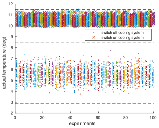
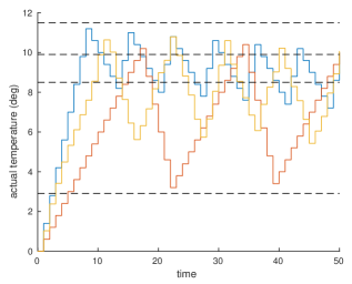
Figure 2: Simulations in MATLAB of the engine $\mathit{Eng}$

In Figure 2, the left graphic collects a campaign of 100 simulations, lasting 250 time units each, showing that the value of the state variable $\mathit{temp}$ when the cooling system is turned on (resp., off) lays in the interval $(9.9,11.5]$ (resp., $(2.9,8.5]$); these bounds are represented by the dashed horizontal lines. Since $\delta=0.4$, these results are in line with those of Proposition 2. The right graphic shows three examples of possible evolutions in time of the state variable $\mathit{temp}$.

Now, the reader may wonder whether it is possible to design a variant of our engine which meets the same specifications with better performances. For instance, an engine consuming less coolant. Let us consider a variant of the engine described before:

$\overline{\mathit{Eng}}\>=\>\overline{\mathit{Env}}\,{\Join}\,\mathit{Ctrl}\enspace.$

Here, $\overline{\mathit{Env}}$ is the same as $\mathit{Env}$ except for the evolution map, as we set $\mathit{heat}(\xi_{\mathrm{u}}^{i}{},\mathit{cool})=-0.8$ if $\xi_{\mathrm{u}}^{i}{}(\mathit{cool})=\mathsf{on}$. This means that in $\overline{\mathit{Eng}}$ we reduce the power of the cooling system by $20\%$. In Figure 3, we report the results of our simulations over $10000$ runs lasting $10000$ time units each. From this graph, $\overline{\mathit{Eng}}$ saves in average more than $10\%$ of coolant with respect to $\mathit{Eng}$. So, the new question is: are these two engines behavioural equivalent? Do they meet the same specifications?

Our bisimilarity provides us with a precise answer to these questions.

Proposition 3

The two variants of the engine are bisimilar: $\mathit{Eng}\approx\overline{\mathit{Eng}}$.

At this point, one may wonder whether it is possible to improve the performances of our engine even more. For instance, by reducing the power of the cooling system by a further $10\%$, by setting $\mathit{heat}(\xi_{\mathrm{u}}^{i}{},\mathit{cool})=-0.7$ if $\xi_{\mathrm{u}}^{i}{}(\mathit{cool})=\mathsf{on}$. We can formally prove that this is not the case.

Proposition 4

Let $\widehat{\mathit{Eng}}$ be the same as $\mathit{Eng}$, except for the evolution map, in which $\mathit{heat}(\xi_{\mathrm{u}}^{i}{},\mathit{cool})=-0.7$ if $\xi_{\mathrm{u}}^{i}{}(\mathit{cool})=\mathsf{on}$. Then, $\mathit{Eng}\not\approx\widehat{\mathit{Eng}}$.

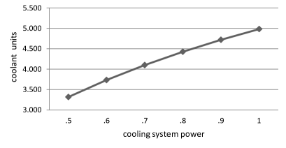
Figure 3: Simulations in MATLAB of coolant consumption

Finally, we show how we can use the compositionality of our behavioural semantics (Theorem 3.1) to deal with bigger CPSs. Suppose that $\mathit{Eng}$ denotes the modelisation of an airplane engine. In this case, we could define in CCPS a very simple airplane control system that checks whether the left engine ($\mathit{Eng}_{\mathrm{L}}$) and the right engine ($\mathit{Eng}_{\mathrm{R}}$) are signalling warnings. The whole CPS is defined as follows:

$$\mathit{Airplane}\>=\>\big{(}(\mathit{Eng}_{\mathrm{L}}\uplus\mathit{Eng}_{\mathrm{R}})\parallel\mathit{Check}\big{)}{\setminus}\{warning\}$$

where $\mathit{Eng}_{\mathrm{L}}=\mathit{Eng}\{^{\mathrm{L}}\!/\!_{\mathrm{ID}}\}\{^{\mathit{temp{\_}l}}\!/\!_{\mathit{temp}}\}\{^{\mathit{cool{\_}l}}\!/\!_{\mathit{cool}}\}\{^{s_{\mathrm{t}{\_}l}}\!/\!_{s_{\mathrm{t}}}\}$, and, similarly, $\mathit{Eng}_{\mathrm{R}}=\mathit{Eng}\{^{\mathrm{R}}\!/\!_{\mathrm{ID}}\}\{^{\mathit{temp{\_}r}}\!/\!_{\mathit{temp}}\}\{^{\mathit{cool{\_}r}}\!/\!_{\mathit{cool}}\}\{^{s_{\mathrm{t}{\_}r}}\!/\!_{s_{\mathrm{t}}}\}$, and process $\mathit{Check}$ is defined as:

$\begin{array}[]{rcl}\mathit{Check}&=&{\mathsf{rec}}\,X.\lfloor\mathsf{rcv}\,\mathit{warning}({x}).[x={\mathrm{L}}]\{\mathit{Check}^{\mathrm{L}}_{1}\},\{\mathit{Check}^{\mathrm{R}}_{1}\}\rfloor X\\[3.0pt] \mathit{Check}^{\mathit{id}}_{i}&=&\lfloor\mathsf{rcv}\,\mathit{warning}({y}).[y\neq{\mathit{id}}]\{\mathsf{snd}\,\mathit{alarm}.\mathsf{idle}.X\},\{\mathsf{idle}.\mathit{Check}^{\mathit{id}}_{i+1}\}\rfloor\mathit{Check}^{\mathit{id}}_{i+1}\\[3.0pt] \mathit{Check}^{\mathit{id}}_{5}&=&\lfloor{\mathsf{rcv}\,\mathit{warning}({z}).[z\neq{\mathit{id}}]\{\mathsf{snd}\,\mathit{alarm}.\mathsf{idle}.X\},\{\mathsf{snd}\,\mathit{failure}\langle{\mathit{id}}\rangle.\mathsf{idle}.X\}}\rfloor\\ &&{\mathsf{snd}\,\mathit{failure}\langle{\mathit{id}}\rangle.X}\end{array}$

for $1\leq i\leq 5$. Intuitively, if one of the two engines is in a warning state then the process $\mathit{Check}^{\mathit{id}}_{i}$, for ${\mathit{id}}\in\{\mathrm{L},\mathrm{R}\}$, checks whether also the second engine moves into a warning state, in the following $5$ time intervals (i.e. during the cooling cycle). If both engines gets in a warning state then an $\mathit{alarm}$ is sent, otherwise, if only one engine is facing a warning then the airplane control system yields a failure signalling which engine is not working properly.

So, since we know that $\mathit{Eng}\approx\overline{\mathit{Eng}}$, the final question becomes the following: can we safely equip our airplane with the more performant engines, $\overline{\mathit{Eng}_{\mathrm{L}}}$ and $\overline{\mathit{Eng}_{\mathrm{R}}}$, in which $\mathit{heat}(\xi_{\mathrm{u}}^{i}{},\mathit{cool})=-0.8$ if $\xi_{\mathrm{u}}^{i}{}(\mathit{cool})=\mathsf{on}$, without affecting the whole observable behaviour of the airplane? The answer is “yes”, and this result can be formally proved by applying Proposition 3 and Theorem 3.1.

Proposition 5

Let $\overline{\mathit{Airplane}}=\big{(}(\overline{\mathit{Eng}_{\mathrm{L}}}\uplus\overline{\mathit{Eng}_{\mathrm{R}}})\parallel\mathit{Check}\big{)}{\setminus}\{warning\}$. Then, $\mathit{Airplane}\approx\overline{\mathit{Airplane}}$.

5 Related and Future Work

A number of approaches have been proposed for modelling CPSs using formal methods. For instance, hybrid automata [1] combine finite state transition systems with discrete variables (whose values capture the state of the modelled discrete or cyber components) and continuous variables (whose values capture the state of the modelled continuous or physical components).

Hybrid process algebras [6] are a powerful tool for reasoning about physical systems and provide techniques for analysing and verifying protocols for hybrid automata. CCPS shares some similarities with the $\phi$-calculus [20], a hybrid extension of the $\pi$-calculus [17]. In the $\phi$-calculus, a hybrid system is represented as a pair $(E,P)$, where $E$ is the environment and $P$ is the process interacting with the environment. Unlike CCPS, in $\phi$-calculus, given a system $(E,P)$ the process $P$ can dynamically change both the evolution law and the invariant of the system. However, the $\phi$-calculus does not have a representation of physical devices and measurement law. Concerning behavioural semantics, the $\phi$-calculus is equipped with a weak bisimilarity between systems that is not compositional.

In the HYPE process algebra [8], the continuous part of the system is represented by appropriate variables whose changes are determined by active influences (i.e., commands on actuators). The authors defines a strong bisimulation that extends the ic-bisimulation of [3]. Unlike ic-bisimulation, the bisimulation in HYPE is preserved by a notion of parallel composition that is slightly more permessive than ours. However, bisimilar systems in HYPE must always have the same influence. Thus, in HYPE we cannot compare CPSs sending different commands on actuators at the same time, as we do in Proposition 3.

Vigo et al. [21] proposed a calculus for wireless-based cyber-physical systems endowed with a theory to study cryptographic primitives, together with explicit notions of communication failure and unwanted communication. The calculus does not provide any notion of behavioural equivalence. It also lacks a clear distinction between physical and logical components.

Lanese et al. [11] proposed an untimed calculus of mobile IoT devices interacting with the physical environment by means of sensors and actuators. The calculus does not allow any representation of the physical environment, and the bisimilarity is not preserved by parallel composition (compositionality is recovered by significantly strengthening the discriminating power).

Lanotte and Merro [13] extended and generalised the work of [11] in a timed setting by providing a bisimulation-based semantic theory that is suitable for compositional reasoning. As in [11], the physical environment is not represented.

Bodei et al. [4] proposed an untimed process calculus supporting a control flow analysis to track how data spread from sensors to the logics of the network, and how physical data are manipulated. Sensors and actuators are modelled as value-passing CCS channels. The dynamics of the calculus is given in terms of a reduction relation and no behavioural equivalence is defined.

As regards future works, we believe that our paper can lay and streamline theoretical foundations for the development of formal and automated tools to verify CPSs before their practical implementation. To that end, we will consider applying, possibly after proper enhancements, existing tools and frameworks for automated verification, such as Maude [18], Ariadne [2], and SMC UPPAAL [7], resorting to the development of an dedicated tool if existing ones prove not up to the task. Finally, in [14], we developed an extended version of CCPS to provide a formal study of a variety of cyber-physical attacks targeting physical devices. Also in this case, the final goal is to develop formal and automated tools to analyse security properties of CPSs.

Acknowledgements

We thank Riccardo Muradore for providing us with simulations in MATLAB.

Appendix 0.A Proofs

We recall that the cyber-components our CPSs are basically TPL-processes [9] extended with constructs to read sensors and write actuators. TPL already enjoys time determinism, patience and maximal progress. The well-timedness property is present in many process calculi with a discrete notion of time (e.g. [15]) similar to ours. Thus, it is straightforward to rewrite the proofs of those results for our slight variant of TPL.

Proposition 6 (Processes time properties [9, 15])

• If $P\mathrel{\;\raisebox{0.0pt}{$\stackrel{{\scriptstyle\,\mathsf{idle}}}{{\makebox[18.55559pt]{\rule{0.0pt}{4.30554pt}\mbox{}\leavevmode\xleaders\hbox{$\mkern-2.6mu\relbar\mkern-2.6mu$}\hfill\mbox{}}}}$}\rightarrow}Q$ and $P\mathrel{\;\raisebox{0.0pt}{$\stackrel{{\scriptstyle\,\mathsf{idle}}}{{\makebox[18.55559pt]{\rule{0.0pt}{4.30554pt}\mbox{}\leavevmode\xleaders\hbox{$\mkern-2.6mu\relbar\mkern-2.6mu$}\hfill\mbox{}}}}$}\rightarrow}{R}$, then $Q\equiv R$.

• If $P\mathrel{\;\raisebox{0.0pt}{$\stackrel{{\scriptstyle\,\tau}}{{\makebox[10.72676pt]{\rule{0.0pt}{4.30554pt}\mbox{}\leavevmode\xleaders\hbox{$\mkern-2.6mu\relbar\mkern-2.6mu$}\hfill\mbox{}}}}$}\rightarrow}P^{\prime}$ then there is no $P^{\prime\prime}$ such that $P\mathrel{\;\raisebox{0.0pt}{$\stackrel{{\scriptstyle\,\mathsf{idle}}}{{\makebox[18.55559pt]{\rule{0.0pt}{4.30554pt}\mbox{}\leavevmode\xleaders\hbox{$\mkern-2.6mu\relbar\mkern-2.6mu$}\hfill\mbox{}}}}$}\rightarrow}P^{\prime\prime}$.

• If $P\mathrel{\;\raisebox{0.0pt}{$\stackrel{{\scriptstyle\,\mathsf{idle}}}{{\makebox[18.55559pt]{\rule{0.0pt}{4.30554pt}\mbox{}\leavevmode\xleaders\hbox{$\mkern-2.6mu\relbar\mkern-2.6mu$}\hfill\mbox{}}}}$}\rightarrow}P^{\prime}$ for no $P^{\prime}$ then there is $Q$ such that $P\mathrel{\;\raisebox{0.0pt}{$\stackrel{{\scriptstyle\,\tau}}{{\makebox[10.72676pt]{\rule{0.0pt}{4.30554pt}\mbox{}\leavevmode\xleaders\hbox{$\mkern-2.6mu\relbar\mkern-2.6mu$}\hfill\mbox{}}}}$}\rightarrow}Q$.

• For any $P$ there is a $k\in\mathbb{N}$ such that if $P\mathrel{\;\raisebox{0.0pt}{$\stackrel{{\scriptstyle\,\lambda_{1}}}{{\makebox[13.75003pt]{\rule{0.0pt}{4.30554pt}\mbox{}\leavevmode\xleaders\hbox{$\mkern-2.6mu\relbar\mkern-2.6mu$}\hfill\mbox{}}}}$}\rightarrow}\dots\mathrel{\;\raisebox{0.0pt}{$\stackrel{{\scriptstyle\,\lambda_{n}}}{{\makebox[14.15097pt]{\rule{0.0pt}{4.30554pt}\mbox{}\leavevmode\xleaders\hbox{$\mkern-2.6mu\relbar\mkern-2.6mu$}\hfill\mbox{}}}}$}\rightarrow}P$, with $\lambda_{i}\neq\mathsf{idle}$, then $n\leq k$.

The challenge in the proof of Theorem 2.1 is to lift the results of Proposition 6 to the CPSs of CCPS.

In its standard formulation, time determinism says that a system reaches at most one new state by executing a $\mathsf{idle}$-action. However, by an application of Rule (Time), our CPSs may nondeterministically move into a new physical environment, according to the evolution law.

Proposition 7 (Time determinism for CPSs)

If $M\mathrel{\;\raisebox{0.0pt}{$\stackrel{{\scriptstyle\,\mathsf{idle}}}{{\makebox[18.55559pt]{\rule{0.0pt}{4.30554pt}\mbox{}\leavevmode\xleaders\hbox{$\mkern-2.6mu\relbar\mkern-2.6mu$}\hfill\mbox{}}}}$}\rightarrow}\hat{E}\,{\Join}\,Q$ and $M\mathrel{\;\raisebox{0.0pt}{$\stackrel{{\scriptstyle\,\mathsf{idle}}}{{\makebox[18.55559pt]{\rule{0.0pt}{4.30554pt}\mbox{}\leavevmode\xleaders\hbox{$\mkern-2.6mu\relbar\mkern-2.6mu$}\hfill\mbox{}}}}$}\rightarrow}\tilde{E}\,{\Join}\,R$, then $\{\hat{E},\tilde{E}\}\subseteq\mathit{next}{(E)}$ and $Q\equiv R$.

Proof

Let $M=E\,{\Join}\,P$. Since the only possible rule to derive $\mathrel{\;\raisebox{0.0pt}{$\stackrel{{\scriptstyle\,\mathsf{idle}}}{{\makebox[18.55559pt]{\rule{0.0pt}{4.30554pt}\mbox{}\leavevmode\xleaders\hbox{$\mkern-2.6mu\relbar\mkern-2.6mu$}\hfill\mbox{}}}}$}\rightarrow}$ is rule (Time), then we have that there is $Q$, $R$, $\hat{E}$, $\tilde{E}$ such that

$$\begin{array}[]{c}P\mathrel{\;\raisebox{0.0pt}{$\stackrel{{\scriptstyle\,\mathsf{idle}}}{{\makebox[18.55559pt]{\rule{0.0pt}{4.30554pt}\mbox{}\leavevmode\xleaders\hbox{$\mkern-2.6mu\relbar\mkern-2.6mu$}\hfill\mbox{}}}}$}\rightarrow}{Q}\>\;\;M\mathrel{{\mathrel{\;\raisebox{0.0pt}{$\stackrel{{\scriptstyle\,\tau}}{{\makebox[10.72676pt]{\rule{0.0pt}{4.30554pt}\mbox{}\leavevmode\xleaders\hbox{$\mkern-2.6mu\relbar\mkern-2.6mu$}\hfill\mbox{}}}}$}\rightarrow}}\makebox[0.0pt][r]{$\not$\hskip 8.61108pt}}{\!}\>\;\;\mathit{inv}{}(E)\>\;\;{\hat{E}}\in\mathit{next}(E)\\[2.0pt] \hline\cr M\mathrel{\;\raisebox{0.0pt}{$\stackrel{{\scriptstyle\,\mathsf{idle}}}{{\makebox[18.55559pt]{\rule{0.0pt}{4.30554pt}\mbox{}\leavevmode\xleaders\hbox{$\mkern-2.6mu\relbar\mkern-2.6mu$}\hfill\mbox{}}}}$}\rightarrow}\hat{E}\,{\Join}\,Q\end{array}$$

and

$$\begin{array}[]{c}P\mathrel{\;\raisebox{0.0pt}{$\stackrel{{\scriptstyle\,\mathsf{idle}}}{{\makebox[18.55559pt]{\rule{0.0pt}{4.30554pt}\mbox{}\leavevmode\xleaders\hbox{$\mkern-2.6mu\relbar\mkern-2.6mu$}\hfill\mbox{}}}}$}\rightarrow}{R}\>\;\;M\mathrel{{\mathrel{\;\raisebox{0.0pt}{$\stackrel{{\scriptstyle\,\tau}}{{\makebox[10.72676pt]{\rule{0.0pt}{4.30554pt}\mbox{}\leavevmode\xleaders\hbox{$\mkern-2.6mu\relbar\mkern-2.6mu$}\hfill\mbox{}}}}$}\rightarrow}}\makebox[0.0pt][r]{$\not$\hskip 8.61108pt}}{\!}\>\;\;\mathit{inv}{}(E)\>\;\;{\tilde{E}}\in\mathit{next}(E)\\[2.0pt] \hline\cr M\mathrel{\;\raisebox{0.0pt}{$\stackrel{{\scriptstyle\,\mathsf{idle}}}{{\makebox[18.55559pt]{\rule{0.0pt}{4.30554pt}\mbox{}\leavevmode\xleaders\hbox{$\mkern-2.6mu\relbar\mkern-2.6mu$}\hfill\mbox{}}}}$}\rightarrow}\tilde{E}\,{\Join}\,R\end{array}\enspace.$$

The result follows by Proposition 6.

According to [9], the maximal progress property says that processes communicate as soon as a possibility of communication arises. In our calculus, we generalise this property saying that $\tau$-actions cannot be delayed, independently on how they are generated.

Proposition 8 (Maximal progress for CPSs)

If $M\mathrel{\;\raisebox{0.0pt}{$\stackrel{{\scriptstyle\,\tau}}{{\makebox[10.72676pt]{\rule{0.0pt}{4.30554pt}\mbox{}\leavevmode\xleaders\hbox{$\mkern-2.6mu\relbar\mkern-2.6mu$}\hfill\mbox{}}}}$}\rightarrow}M^{\prime}$ then there is no $M^{\prime\prime}$ such that $M\mathrel{\;\raisebox{0.0pt}{$\stackrel{{\scriptstyle\,\mathsf{idle}}}{{\makebox[18.55559pt]{\rule{0.0pt}{4.30554pt}\mbox{}\leavevmode\xleaders\hbox{$\mkern-2.6mu\relbar\mkern-2.6mu$}\hfill\mbox{}}}}$}\rightarrow}M^{\prime\prime}$.

Proof

The proof is by contradiction. Let us suppose $M\mathrel{\;\raisebox{0.0pt}{$\stackrel{{\scriptstyle\,\mathsf{idle}}}{{\makebox[18.55559pt]{\rule{0.0pt}{4.30554pt}\mbox{}\leavevmode\xleaders\hbox{$\mkern-2.6mu\relbar\mkern-2.6mu$}\hfill\mbox{}}}}$}\rightarrow}M^{\prime\prime}$, for some $M^{\prime\prime}$. This is only possible by an application of rule (Time):

$$\begin{array}[]{c}P\mathrel{\;\raisebox{0.0pt}{$\stackrel{{\scriptstyle\,\mathsf{idle}}}{{\makebox[18.55559pt]{\rule{0.0pt}{4.30554pt}\mbox{}\leavevmode\xleaders\hbox{$\mkern-2.6mu\relbar\mkern-2.6mu$}\hfill\mbox{}}}}$}\rightarrow}{P^{\prime}}\>\;\;M\mathrel{{\mathrel{\;\raisebox{0.0pt}{$\stackrel{{\scriptstyle\,\tau}}{{\makebox[10.72676pt]{\rule{0.0pt}{4.30554pt}\mbox{}\leavevmode\xleaders\hbox{$\mkern-2.6mu\relbar\mkern-2.6mu$}\hfill\mbox{}}}}$}\rightarrow}}\makebox[0.0pt][r]{$\not$\hskip 8.61108pt}}{\!}\>\;\;\mathit{inv}{}(E)\>\;\;E^{\prime}\in\mathit{next}(E)\\[2.0pt] \hline\cr M\mathrel{\;\raisebox{0.0pt}{$\stackrel{{\scriptstyle\,\mathsf{idle}}}{{\makebox[18.55559pt]{\rule{0.0pt}{4.30554pt}\mbox{}\leavevmode\xleaders\hbox{$\mkern-2.6mu\relbar\mkern-2.6mu$}\hfill\mbox{}}}}$}\rightarrow}M^{\prime\prime}\end{array}$$

with $M^{\prime\prime}=E^{\prime}\,{\Join}\,P^{\prime}$. However, the premises requires $M\mathrel{{\mathrel{\;\raisebox{0.0pt}{$\stackrel{{\scriptstyle\,\tau}}{{\makebox[10.72676pt]{\rule{0.0pt}{4.30554pt}\mbox{}\leavevmode\xleaders\hbox{$\mkern-2.6mu\relbar\mkern-2.6mu$}\hfill\mbox{}}}}$}\rightarrow}}\makebox[0.0pt][r]{$\not$\hskip 8.61108pt}}{\!}$ which contradicts the fact that $M\mathrel{\;\raisebox{0.0pt}{$\stackrel{{\scriptstyle\,\tau}}{{\makebox[10.72676pt]{\rule{0.0pt}{4.30554pt}\mbox{}\leavevmode\xleaders\hbox{$\mkern-2.6mu\relbar\mkern-2.6mu$}\hfill\mbox{}}}}$}\rightarrow}M^{\prime}$.

Patience in CCPS is more involved with respect to the same property in TPL. It basically says that if a CPS cannot evolve in time, then either (i) the physical plant does not contemplate an evolution, or (ii) the invariant is violated, or (iii) the CPS can perform an internal action.

Proposition 9 (Patience for CPS)

If $M\mathrel{\;\raisebox{0.0pt}{$\stackrel{{\scriptstyle\,\mathsf{idle}}}{{\makebox[18.55559pt]{\rule{0.0pt}{4.30554pt}\mbox{}\leavevmode\xleaders\hbox{$\mkern-2.6mu\relbar\mkern-2.6mu$}\hfill\mbox{}}}}$}\rightarrow}M^{\prime}$ for no $M^{\prime}$ then either $\mathit{next}(E)=\emptyset$ or $\mathit{inv}{(M)}=\mathsf{false}$ or there is $N$ such that $M\mathrel{\;\raisebox{0.0pt}{$\stackrel{{\scriptstyle\,\tau}}{{\makebox[10.72676pt]{\rule{0.0pt}{4.30554pt}\mbox{}\leavevmode\xleaders\hbox{$\mkern-2.6mu\relbar\mkern-2.6mu$}\hfill\mbox{}}}}$}\rightarrow}N$.

Proof

The proof is by contradiction. Let us suppose that $M\mathrel{\;\raisebox{0.0pt}{$\stackrel{{\scriptstyle\,\mathsf{idle}}}{{\makebox[18.55559pt]{\rule{0.0pt}{4.30554pt}\mbox{}\leavevmode\xleaders\hbox{$\mkern-2.6mu\relbar\mkern-2.6mu$}\hfill\mbox{}}}}$}\rightarrow}M^{\prime}$ for no $M^{\prime}$, and $M\mathrel{{\mathrel{\;\raisebox{0.0pt}{$\stackrel{{\scriptstyle\,\tau}}{{\makebox[10.72676pt]{\rule{0.0pt}{4.30554pt}\mbox{}\leavevmode\xleaders\hbox{$\mkern-2.6mu\relbar\mkern-2.6mu$}\hfill\mbox{}}}}$}\rightarrow}}\makebox[0.0pt][r]{$\not$\hskip 8.61108pt}}{\!}$ and $\mathit{inv}{}(E)=\mathsf{true}$ and $E^{\prime}\in\mathit{next}(E)$, for some $E^{\prime}$. Since the only possible rule to derive $\mathrel{\;\raisebox{0.0pt}{$\stackrel{{\scriptstyle\,\mathsf{idle}}}{{\makebox[18.55559pt]{\rule{0.0pt}{4.30554pt}\mbox{}\leavevmode\xleaders\hbox{$\mkern-2.6mu\relbar\mkern-2.6mu$}\hfill\mbox{}}}}$}\rightarrow}$ is rule (Time), then $M\mathrel{\;\raisebox{0.0pt}{$\stackrel{{\scriptstyle\,\mathsf{idle}}}{{\makebox[18.55559pt]{\rule{0.0pt}{4.30554pt}\mbox{}\leavevmode\xleaders\hbox{$\mkern-2.6mu\relbar\mkern-2.6mu$}\hfill\mbox{}}}}$}\rightarrow}M^{\prime}$ for no $M^{\prime}$, implies that the following derivation is not admissible for any $P^{\prime}$ and $E^{\prime}$:

$$\begin{array}[]{c}P\mathrel{\;\raisebox{0.0pt}{$\stackrel{{\scriptstyle\,\mathsf{idle}}}{{\makebox[18.55559pt]{\rule{0.0pt}{4.30554pt}\mbox{}\leavevmode\xleaders\hbox{$\mkern-2.6mu\relbar\mkern-2.6mu$}\hfill\mbox{}}}}$}\rightarrow}{P^{\prime}}\>\;\;M\mathrel{{\mathrel{\;\raisebox{0.0pt}{$\stackrel{{\scriptstyle\,\tau}}{{\makebox[10.72676pt]{\rule{0.0pt}{4.30554pt}\mbox{}\leavevmode\xleaders\hbox{$\mkern-2.6mu\relbar\mkern-2.6mu$}\hfill\mbox{}}}}$}\rightarrow}}\makebox[0.0pt][r]{$\not$\hskip 8.61108pt}}{\!}\>\;\;\mathit{inv}{}(E)\>\;\;E^{\prime}{\in}\mathit{next}(E)\\[2.0pt] \hline\cr M\mathrel{\;\raisebox{0.0pt}{$\stackrel{{\scriptstyle\,\mathsf{idle}}}{{\makebox[18.55559pt]{\rule{0.0pt}{4.30554pt}\mbox{}\leavevmode\xleaders\hbox{$\mkern-2.6mu\relbar\mkern-2.6mu$}\hfill\mbox{}}}}$}\rightarrow}E^{\prime}\,{\Join}\,P^{\prime}\end{array}\enspace.$$

Since $M\mathrel{{\mathrel{\;\raisebox{0.0pt}{$\stackrel{{\scriptstyle\,\tau}}{{\makebox[10.72676pt]{\rule{0.0pt}{4.30554pt}\mbox{}\leavevmode\xleaders\hbox{$\mkern-2.6mu\relbar\mkern-2.6mu$}\hfill\mbox{}}}}$}\rightarrow}}\makebox[0.0pt][r]{$\not$\hskip 8.61108pt}}{\!}$ and $\mathit{inv}{}(E)=\mathsf{true}$ and $E^{\prime}\in\mathit{next}(E)$, for some $E^{\prime}$, the only possibility is $P\mathrel{\;\raisebox{0.0pt}{$\stackrel{{\scriptstyle\,\mathsf{idle}}}{{\makebox[18.55559pt]{\rule{0.0pt}{4.30554pt}\mbox{}\leavevmode\xleaders\hbox{$\mkern-2.6mu\relbar\mkern-2.6mu$}\hfill\mbox{}}}}$}\rightarrow}{P^{\prime}}$ for no $P^{\prime}$. Since $P\mathrel{\;\raisebox{0.0pt}{$\stackrel{{\scriptstyle\,\mathsf{idle}}}{{\makebox[18.55559pt]{\rule{0.0pt}{4.30554pt}\mbox{}\leavevmode\xleaders\hbox{$\mkern-2.6mu\relbar\mkern-2.6mu$}\hfill\mbox{}}}}$}\rightarrow}{P^{\prime}}$ for no $P^{\prime}$, by Proposition 6 we have that $P\mathrel{\;\raisebox{0.0pt}{$\stackrel{{\scriptstyle\,\tau}}{{\makebox[10.72676pt]{\rule{0.0pt}{4.30554pt}\mbox{}\leavevmode\xleaders\hbox{$\mkern-2.6mu\relbar\mkern-2.6mu$}\hfill\mbox{}}}}$}\rightarrow}{P^{\prime}}$. Since $\mathit{inv}{}(E)=\mathsf{true}$, by an application of rule (Tau) there is $N$ such that $M\mathrel{\;\raisebox{0.0pt}{$\stackrel{{\scriptstyle\,\tau}}{{\makebox[10.72676pt]{\rule{0.0pt}{4.30554pt}\mbox{}\leavevmode\xleaders\hbox{$\mkern-2.6mu\relbar\mkern-2.6mu$}\hfill\mbox{}}}}$}\rightarrow}N$. This contradicts the initial hypothesis that $M\mathrel{{\mathrel{\;\raisebox{0.0pt}{$\stackrel{{\scriptstyle\,\tau}}{{\makebox[10.72676pt]{\rule{0.0pt}{4.30554pt}\mbox{}\leavevmode\xleaders\hbox{$\mkern-2.6mu\relbar\mkern-2.6mu$}\hfill\mbox{}}}}$}\rightarrow}}\makebox[0.0pt][r]{$\not$\hskip 8.61108pt}}{\!}$. [5, 16, 12]

The following property is well-timedness. It basically says that time passing cannot be prevented by infinite sequences of internal actions.

Proposition 10 (Well-timedness for CPSs)

For any $M$ there is a $k\in\mathbb{N}$ such that if $M\mathrel{\;\raisebox{0.0pt}{$\stackrel{{\scriptstyle\,\alpha_{1}}}{{\makebox[14.14459pt]{\rule{0.0pt}{4.30554pt}\mbox{}\leavevmode\xleaders\hbox{$\mkern-2.6mu\relbar\mkern-2.6mu$}\hfill\mbox{}}}}$}\rightarrow}\dots\mathrel{\;\raisebox{0.0pt}{$\stackrel{{\scriptstyle\,\alpha_{n}}}{{\makebox[14.54553pt]{\rule{0.0pt}{4.30554pt}\mbox{}\leavevmode\xleaders\hbox{$\mkern-2.6mu\relbar\mkern-2.6mu$}\hfill\mbox{}}}}$}\rightarrow}N$, with $\alpha_{i}\neq\mathsf{idle}$, then $n\leq k$.

Proof

The proof is by contradiction. Suppose there is no $k$ satisfying the statement above. Hence there exists an unbounded derivation

$$M=M_{1}\mathrel{\;\raisebox{0.0pt}{$\stackrel{{\scriptstyle\,\alpha_{1}}}{{\makebox[14.14459pt]{\rule{0.0pt}{4.30554pt}\mbox{}\leavevmode\xleaders\hbox{$\mkern-2.6mu\relbar\mkern-2.6mu$}\hfill\mbox{}}}}$}\rightarrow}\dots\mathrel{\;\raisebox{0.0pt}{$\stackrel{{\scriptstyle\,\alpha_{n}}}{{\makebox[14.54553pt]{\rule{0.0pt}{4.30554pt}\mbox{}\leavevmode\xleaders\hbox{$\mkern-2.6mu\relbar\mkern-2.6mu$}\hfill\mbox{}}}}$}\rightarrow}M_{n+1}\mathrel{\;\raisebox{0.0pt}{$\stackrel{{\scriptstyle\,\alpha_{n+1}}}{{\makebox[19.65665pt]{\rule{0.0pt}{4.30554pt}\mbox{}\leavevmode\xleaders\hbox{$\mkern-2.6mu\relbar\mkern-2.6mu$}\hfill\mbox{}}}}$}\rightarrow}\dots$$

with $M_{i}=E_{i}\,{\Join}\,P_{i}$ and $\alpha_{i}\neq\mathsf{idle}$.

By inspection of rules of Table 2 we have that, for any $i$, $M_{i}\mathrel{\;\raisebox{0.0pt}{$\stackrel{{\scriptstyle\,\alpha_{i}}}{{\makebox[13.52264pt]{\rule{0.0pt}{4.30554pt}\mbox{}\leavevmode\xleaders\hbox{$\mkern-2.6mu\relbar\mkern-2.6mu$}\hfill\mbox{}}}}$}\rightarrow}M_{i+1}$ and $\alpha_{i}\neq\mathsf{idle}$ implies that $P_{i}\mathrel{\;\raisebox{0.0pt}{$\stackrel{{\scriptstyle\,\lambda_{i}}}{{\makebox[13.12808pt]{\rule{0.0pt}{4.30554pt}\mbox{}\leavevmode\xleaders\hbox{$\mkern-2.6mu\relbar\mkern-2.6mu$}\hfill\mbox{}}}}$}\rightarrow}P_{i+1}$, for some $\lambda_{i}\neq\mathsf{idle}$. Hence we have the following unbounded derivation

$$P_{1}\mathrel{\;\raisebox{0.0pt}{$\stackrel{{\scriptstyle\,\lambda_{1}}}{{\makebox[13.75003pt]{\rule{0.0pt}{4.30554pt}\mbox{}\leavevmode\xleaders\hbox{$\mkern-2.6mu\relbar\mkern-2.6mu$}\hfill\mbox{}}}}$}\rightarrow}\dots\mathrel{\;\raisebox{0.0pt}{$\stackrel{{\scriptstyle\,\lambda_{n}}}{{\makebox[14.15097pt]{\rule{0.0pt}{4.30554pt}\mbox{}\leavevmode\xleaders\hbox{$\mkern-2.6mu\relbar\mkern-2.6mu$}\hfill\mbox{}}}}$}\rightarrow}P_{n+1}\mathrel{\;\raisebox{0.0pt}{$\stackrel{{\scriptstyle\,\lambda_{n+1}}}{{\makebox[19.26208pt]{\rule{0.0pt}{4.30554pt}\mbox{}\leavevmode\xleaders\hbox{$\mkern-2.6mu\relbar\mkern-2.6mu$}\hfill\mbox{}}}}$}\rightarrow}\dots$$

with $\lambda_{i}\neq\mathsf{idle}$. In contradiction with Proposition 6.

Proof of Theorem 2.1

Proof

The result follows by an application of Proposition 7, Proposition 8, Proposition 9 and Proposition 10.

In order to prove the compositionality or our bisimilarity, i.e. Theorem 3.1, we divide its statement in three different propositions.

In order to prove that $\approx$ preserves contextuality, we need a number of technical lemmas. Lemma 1 formalises a number of properties of the compound environment $E_{1}\uplus E_{2}$.

Lemma 1

Let $E_{1}$ and $E_{2}$ be two physical environments. If defined, the environment $E_{1}\uplus E_{2}$ has the following properties:

1. $\mathit{read\_sensor}(E_{1}\uplus E_{2},s)$ is equal to $\mathit{read\_sensor}(E_{1},s)$, if $s$ is a sensor of $E_{1}$, and it is equal to $\mathit{read\_sensor}(E_{2},s)$, if $s$ is a sensor of $E_{2}$;

2. $v\in\mathit{read\_sensor}(E_{1},s)$ implies that $v\in\mathit{read\_sensor}(E_{1}\uplus E_{2},s)$ for any sensor $s$ in $E_{1}$ and for any environment $E_{2}$;

3. $\mathit{update\_act}(E_{1}\uplus E_{2},a,v)$ is equal to $\mathit{update\_act}(E_{1},a,v)\uplus E_{2}$, if $a$ is an actuator of $E_{1}$, and it is equal to $E_{1}\uplus\mathit{update\_act}(E_{2},a,v)$, if $a$ is an actuator of $E_{2}$;

4. $\mathit{update\_act}(E_{1},a,v)\uplus E_{2}$ is equal to $\mathit{update\_act}(E_{1}\uplus E_{2},a,v)$ for any actuator $a$ in $E_{1}$ and for any environment $E_{2}$;

5. $\mathit{next}(E_{1}\uplus E_{2})=\{\,E_{1}^{\prime}\uplus E_{2}^{\prime}\,:\,E_{1}^{\prime}\in\mathit{next}(E_{1})\mbox{ and }E_{2}^{\prime}\in\mathit{next}(E_{2})\,\}$;

6. $\mathit{inv}{}(E_{1}\uplus E_{2})=\mathit{inv}{}(E_{1})\wedge\mathit{inv}{}(E_{2})$.

Proof

By definition of the operator $\uplus$ on physical environments.

Lemma 2 serves to propagate untimed actions on parallel CPSs.

Lemma 2

If $M\mathrel{\;\raisebox{0.0pt}{$\stackrel{{\scriptstyle\,\alpha}}{{\makebox[12.14459pt]{\rule{0.0pt}{4.30554pt}\mbox{}\leavevmode\xleaders\hbox{$\mkern-2.6mu\relbar\mkern-2.6mu$}\hfill\mbox{}}}}$}\rightarrow}M^{\prime}$, with $\alpha\neq\mathsf{idle}$, then $M\uplus O\mathrel{\;\raisebox{0.0pt}{$\stackrel{{\scriptstyle\,\alpha}}{{\makebox[12.14459pt]{\rule{0.0pt}{4.30554pt}\mbox{}\leavevmode\xleaders\hbox{$\mkern-2.6mu\relbar\mkern-2.6mu$}\hfill\mbox{}}}}$}\rightarrow}M^{\prime}\uplus O$, for any non-interfering CPS $O$, with $\mathit{inv}{}(O)=\mathsf{true}$.

Proof

The proof is by rule induction on why $M\mathrel{\;\raisebox{0.0pt}{$\stackrel{{\scriptstyle\,\alpha}}{{\makebox[12.14459pt]{\rule{0.0pt}{4.30554pt}\mbox{}\leavevmode\xleaders\hbox{$\mkern-2.6mu\relbar\mkern-2.6mu$}\hfill\mbox{}}}}$}\rightarrow}M^{\prime}$. Let us suppose that $M=E_{1}\,{\Join}\,P_{1}$ and $O=E_{2}\,{\Join}\,P_{2}$, for some $E_{1}$, $E_{2}$, $P_{1}$ and $P_{2}$. We can distinguish several cases on why $M\mathrel{\;\raisebox{0.0pt}{$\stackrel{{\scriptstyle\,\alpha}}{{\makebox[12.14459pt]{\rule{0.0pt}{4.30554pt}\mbox{}\leavevmode\xleaders\hbox{$\mkern-2.6mu\relbar\mkern-2.6mu$}\hfill\mbox{}}}}$}\rightarrow}M^{\prime}$. We prove the case in which $M\mathrel{\;\raisebox{0.0pt}{$\stackrel{{\scriptstyle\,\alpha}}{{\makebox[12.14459pt]{\rule{0.0pt}{4.30554pt}\mbox{}\leavevmode\xleaders\hbox{$\mkern-2.6mu\relbar\mkern-2.6mu$}\hfill\mbox{}}}}$}\rightarrow}M^{\prime}$ is derived by an application of rule (SensRead). The other cases can be proved in a similar manner. In this case, we have $\alpha=\tau$ and there are $s$, $v$, and $P^{\prime}_{1}$ such that

$$\begin{array}[]{c}P_{1}\mathrel{\;\raisebox{0.0pt}{$\stackrel{{\scriptstyle\,s?v}}{{\makebox[17.8977pt]{\rule{0.0pt}{4.30554pt}\mbox{}\leavevmode\xleaders\hbox{$\mkern-2.6mu\relbar\mkern-2.6mu$}\hfill\mbox{}}}}$}\rightarrow}P_{1}^{\prime}\quad\mathit{inv}{}(E_{1})\quad\mbox{\small{$v\in\mathit{read\_sensor}(E_{1},s)$}}\\[2.0pt] \hline\cr M\mathrel{\;\raisebox{0.0pt}{$\stackrel{{\scriptstyle\,\tau}}{{\makebox[10.72676pt]{\rule{0.0pt}{4.30554pt}\mbox{}\leavevmode\xleaders\hbox{$\mkern-2.6mu\relbar\mkern-2.6mu$}\hfill\mbox{}}}}$}\rightarrow}M^{\prime}\end{array}$$

with $M^{\prime}=E_{1}\,{\Join}\,P^{\prime}_{1}$.

Since $P_{1}\mathrel{\;\raisebox{0.0pt}{$\stackrel{{\scriptstyle\,s?v}}{{\makebox[17.8977pt]{\rule{0.0pt}{4.30554pt}\mbox{}\leavevmode\xleaders\hbox{$\mkern-2.6mu\relbar\mkern-2.6mu$}\hfill\mbox{}}}}$}\rightarrow}P^{\prime}_{1}$, by an applicaiton of rule (Par) we can derive $P_{1}\parallel P_{2}\mathrel{\;\raisebox{0.0pt}{$\stackrel{{\scriptstyle\,s?v}}{{\makebox[17.8977pt]{\rule{0.0pt}{4.30554pt}\mbox{}\leavevmode\xleaders\hbox{$\mkern-2.6mu\relbar\mkern-2.6mu$}\hfill\mbox{}}}}$}\rightarrow}P^{\prime}_{1}\parallel P_{2}$. Since $\mathit{inv}{}(E_{1})=\mathsf{true}$ and, by hypothesis, $\mathit{inv}{}(E_{2})=\mathsf{true}$, by an application of Lemma 1(6) we derive that $\mathit{inv}{}(E_{1}\uplus E_{2})=\mathsf{true}$. Since $v\in\mathit{read\_sensor}(E_{1},s)$, by an application of Lemma 1(2) we derive that $v\in\mathit{read\_sensor}(E_{1}\uplus E_{2},s)$. This is enough to derive that:

$$\begin{array}[]{c}P_{1}\parallel P_{2}\mathrel{\;\raisebox{0.0pt}{$\stackrel{{\scriptstyle\,s?v}}{{\makebox[17.8977pt]{\rule{0.0pt}{4.30554pt}\mbox{}\leavevmode\xleaders\hbox{$\mkern-2.6mu\relbar\mkern-2.6mu$}\hfill\mbox{}}}}$}\rightarrow}P^{\prime}_{1}\parallel P_{2}\quad\mathit{inv}{}(E_{1}\uplus E_{2})\quad\mbox{\small{$v\in\mathit{read\_sensor}(E_{1}\uplus E_{2},s)$}}\\[2.0pt] \hline\cr M\uplus O\mathrel{\;\raisebox{0.0pt}{$\stackrel{{\scriptstyle\,\tau}}{{\makebox[10.72676pt]{\rule{0.0pt}{4.30554pt}\mbox{}\leavevmode\xleaders\hbox{$\mkern-2.6mu\relbar\mkern-2.6mu$}\hfill\mbox{}}}}$}\rightarrow}E_{1}\uplus E_{2}\,{\Join}\,P^{\prime}_{1}\parallel P_{2}\end{array}\enspace.$$

Hence the result follows by assuming $M^{\prime}=E_{1}\,{\Join}\,P^{\prime}$ and $M^{\prime}\uplus O=E_{1}\uplus E_{2}\,{\Join}\,P^{\prime}_{1}\parallel P_{2}$.

Next lemma says the invariants of bisimilar CPSs must agree.

Lemma 3

$M\approx N$ implies $\mathit{inv}{}(M)=\mathit{inv}{}(N)$.

Proof

The proof is by contradiction. Suppose that $M\approx N$, $\mathit{inv}{}(M)=\mathsf{true}$ and $\mathit{inv}{}(N)=\mathsf{false}$ (the other case is similar). By Proposition 10, there exists a finite derivation $M\mathrel{\;\raisebox{0.0pt}{$\stackrel{{\scriptstyle\,\tau}}{{\makebox[10.72676pt]{\rule{0.0pt}{4.30554pt}\mbox{}\leavevmode\xleaders\hbox{$\mkern-2.6mu\relbar\mkern-2.6mu$}\hfill\mbox{}}}}$}\rightarrow}M_{1}\mathrel{\;\raisebox{0.0pt}{$\stackrel{{\scriptstyle\,\tau}}{{\makebox[10.72676pt]{\rule{0.0pt}{4.30554pt}\mbox{}\leavevmode\xleaders\hbox{$\mkern-2.6mu\relbar\mkern-2.6mu$}\hfill\mbox{}}}}$}\rightarrow}\dots\mathrel{\;\raisebox{0.0pt}{$\stackrel{{\scriptstyle\,\tau}}{{\makebox[10.72676pt]{\rule{0.0pt}{4.30554pt}\mbox{}\leavevmode\xleaders\hbox{$\mkern-2.6mu\relbar\mkern-2.6mu$}\hfill\mbox{}}}}$}\rightarrow}M_{n}$, with $M_{n}\mathrel{{\mathrel{\;\raisebox{0.0pt}{$\stackrel{{\scriptstyle\,\tau}}{{\makebox[10.72676pt]{\rule{0.0pt}{4.30554pt}\mbox{}\leavevmode\xleaders\hbox{$\mkern-2.6mu\relbar\mkern-2.6mu$}\hfill\mbox{}}}}$}\rightarrow}}\makebox[0.0pt][r]{$\not$\hskip 8.61108pt}}{\!}$. Since $\mathit{inv}{}(N)=\mathsf{false}$, the CPSs $N$ cannot perform any action, and in particular, $N\mathrel{{\mathrel{\;\raisebox{0.0pt}{$\stackrel{{\scriptstyle\,\tau}}{{\makebox[10.72676pt]{\rule{0.0pt}{4.30554pt}\mbox{}\leavevmode\xleaders\hbox{$\mkern-2.6mu\relbar\mkern-2.6mu$}\hfill\mbox{}}}}$}\rightarrow}}\makebox[0.0pt][r]{$\not$\hskip 8.61108pt}}{\!}$. From $M\approx N$ we derive that $M_{i}\approx N$, for $1\leq i\leq n$. Since $M_{n}\mathrel{{\mathrel{\;\raisebox{0.0pt}{$\stackrel{{\scriptstyle\,\tau}}{{\makebox[10.72676pt]{\rule{0.0pt}{4.30554pt}\mbox{}\leavevmode\xleaders\hbox{$\mkern-2.6mu\relbar\mkern-2.6mu$}\hfill\mbox{}}}}$}\rightarrow}}\makebox[0.0pt][r]{$\not$\hskip 8.61108pt}}{\!}$, by Proposition 8 it follows that $M_{n}\mathrel{\;\raisebox{0.0pt}{$\stackrel{{\scriptstyle\,\mathsf{idle}}}{{\makebox[18.55559pt]{\rule{0.0pt}{4.30554pt}\mbox{}\leavevmode\xleaders\hbox{$\mkern-2.6mu\relbar\mkern-2.6mu$}\hfill\mbox{}}}}$}\rightarrow}M^{\prime}$, for some $M^{\prime}$. Since $\mathit{inv}{}(N)=\mathsf{false}$ , we have $N\mathrel{{\mathrel{\;\raisebox{0.0pt}{$\stackrel{{\scriptstyle\,\mathsf{idle}}}{{\makebox[18.55559pt]{\rule{0.0pt}{4.30554pt}\mbox{}\leavevmode\xleaders\hbox{$\mkern-2.6mu\relbar\mkern-2.6mu$}\hfill\mbox{}}}}$}\rightarrow}}\makebox[0.0pt][r]{$\not$\hskip 8.61108pt}}{\!}$ and hene also $N\not\!\!\!\!\mathrel{\;\raisebox{0.0pt}{$\stackrel{{\scriptstyle\,\mathsf{idle}}}{{\makebox[18.55559pt]{\mbox{}\leavevmode\xleaders\hbox{$\mkern-2.6mu\Relbar\mkern-2.6mu$}\hfill\mbox{}}}}$}\Rightarrow}$.

Summarising: $M_{n}\approx N$, $M_{n}\mathrel{\;\raisebox{0.0pt}{$\stackrel{{\scriptstyle\,\mathsf{idle}}}{{\makebox[18.55559pt]{\rule{0.0pt}{4.30554pt}\mbox{}\leavevmode\xleaders\hbox{$\mkern-2.6mu\relbar\mkern-2.6mu$}\hfill\mbox{}}}}$}\rightarrow}M^{\prime}$ and $N\not\!\!\!\!\mathrel{\;\raisebox{0.0pt}{$\stackrel{{\scriptstyle\,\mathsf{idle}}}{{\makebox[18.55559pt]{\mbox{}\leavevmode\xleaders\hbox{$\mkern-2.6mu\Relbar\mkern-2.6mu$}\hfill\mbox{}}}}$}\Rightarrow}$ which contradict the definition of bisimilarity.

Here comes one of the main technical result: the bisimilarity is preserved by the parallel composition of non-interfering CPSs.

Proposition 11

$M\approx N$ implies $M\uplus O\approx N\uplus O$, for any non-interfering CPS $O$.

Proof

We show that the relation $\mathcal{R}=\mathcal{R}_{1}\cup\mathcal{R}_{2}$ is a bisimulation where:

$$\begin{array}[]{rcl}\mathcal{R}_{1}&=&\left\{(M\uplus O,\;N\uplus O):M\approx N\right\}\\[2.0pt] \mathcal{R}_{2}&=&\left\{(M,N):\mathit{inv}{}(M)=\mathit{inv}{}(N)=\mathsf{false}\right\}\enspace.\end{array}$$

The relation $\mathcal{R}_{2}$ is trivially a bisimulation because it contains pairs of deadlocked CPSs. Thus, we focus on when $(M\uplus O,\;N\uplus O)\in\mathcal{R}_{1}$.

We proceed by case analysis on why $M\uplus O\mathrel{\;\raisebox{0.0pt}{$\stackrel{{\scriptstyle\,\alpha}}{{\makebox[12.14459pt]{\rule{0.0pt}{4.30554pt}\mbox{}\leavevmode\xleaders\hbox{$\mkern-2.6mu\relbar\mkern-2.6mu$}\hfill\mbox{}}}}$}\rightarrow}\hat{M}$ (the case when $N\uplus O\mathrel{\;\raisebox{0.0pt}{$\stackrel{{\scriptstyle\,\alpha}}{{\makebox[12.14459pt]{\rule{0.0pt}{4.30554pt}\mbox{}\leavevmode\xleaders\hbox{$\mkern-2.6mu\relbar\mkern-2.6mu$}\hfill\mbox{}}}}$}\rightarrow}\hat{N}$ is symmetric).

• Let $M\uplus O\mathrel{\;\raisebox{0.0pt}{$\stackrel{{\scriptstyle\,\tau}}{{\makebox[10.72676pt]{\rule{0.0pt}{4.30554pt}\mbox{}\leavevmode\xleaders\hbox{$\mkern-2.6mu\relbar\mkern-2.6mu$}\hfill\mbox{}}}}$}\rightarrow}\hat{M}$, with $M=E_{1}\,{\Join}\,P_{1}$ and $O=E_{2}\,{\Join}\,P_{2}$, for some $E_{1}$, $E_{2}$, $P_{1}$ and $P_{2}$, by an application of rule (SensRead). This implies that

  $$\begin{array}[]{c}P_{1}\parallel P_{2}\mathrel{\;\raisebox{0.0pt}{$\stackrel{{\scriptstyle\,s?v}}{{\makebox[17.8977pt]{\rule{0.0pt}{4.30554pt}\mbox{}\leavevmode\xleaders\hbox{$\mkern-2.6mu\relbar\mkern-2.6mu$}\hfill\mbox{}}}}$}\rightarrow}P^{\prime}\quad\mathit{inv}{}(E_{1}\uplus E_{2})\quad\mbox{\small{$v\in\mathit{read\_sensor}(E_{1}\uplus E_{2},s)$}}\\[2.0pt] \hline\cr M\uplus O\mathrel{\;\raisebox{0.0pt}{$\stackrel{{\scriptstyle\,\tau}}{{\makebox[10.72676pt]{\rule{0.0pt}{4.30554pt}\mbox{}\leavevmode\xleaders\hbox{$\mkern-2.6mu\relbar\mkern-2.6mu$}\hfill\mbox{}}}}$}\rightarrow}\hat{M}\end{array}$$

  with $\hat{M}=E_{1}\uplus E_{2}\,{\Join}\,P^{\prime}$. We recall that by definition of $\uplus$ the environments $E_{1}$ and $E_{2}$ have different physical devices. Thus, there are two cases:

  • $s$ is a sensor of $E_{1}$.

    In this case, $P_{1}\mathrel{\;\raisebox{0.0pt}{$\stackrel{{\scriptstyle\,s?v}}{{\makebox[17.8977pt]{\rule{0.0pt}{4.30554pt}\mbox{}\leavevmode\xleaders\hbox{$\mkern-2.6mu\relbar\mkern-2.6mu$}\hfill\mbox{}}}}$}\rightarrow}P^{\prime}_{1}$, for some $P^{\prime}_{1}$, and hence $P^{\prime}=P^{\prime}_{1}\parallel P_{2}$. Since $\mathit{inv}{}(E_{1}\uplus E_{2})=\mathsf{true}$ and $v\in\mathit{read\_sensor}(E_{1}\uplus E_{2},s)$, by an application of Lemma 1(1) and Lemma 1(6), we derive $\mathit{inv}{}(E_{1})=\mathit{inv}{}(E_{2})=\mathsf{true}$ and $v\in\mathit{read\_sensor}(E_{1},s)$. Now, let $M^{\prime}=E_{1}\,{\Join}\,P_{1}^{\prime}$; it follows that $\hat{M}=M^{\prime}\uplus O$. Since $P_{1}\mathrel{\;\raisebox{0.0pt}{$\stackrel{{\scriptstyle\,s?v}}{{\makebox[17.8977pt]{\rule{0.0pt}{4.30554pt}\mbox{}\leavevmode\xleaders\hbox{$\mkern-2.6mu\relbar\mkern-2.6mu$}\hfill\mbox{}}}}$}\rightarrow}P^{\prime}_{1}$, $\mathit{inv}{}(E_{1})=\mathsf{true}$, and $v\in\mathit{read\_sensor}(E_{1},s)$, by an application of rule (SensRead) we have $M\mathrel{\;\raisebox{0.0pt}{$\stackrel{{\scriptstyle\,\tau}}{{\makebox[10.72676pt]{\rule{0.0pt}{4.30554pt}\mbox{}\leavevmode\xleaders\hbox{$\mkern-2.6mu\relbar\mkern-2.6mu$}\hfill\mbox{}}}}$}\rightarrow}M^{\prime}$. As $M\approx N$, there is $N^{\prime}$ such that $N\mathrel{\;\raisebox{0.0pt}{$\stackrel{{\scriptstyle\,}}{{\makebox[7.66669pt]{\mbox{}\leavevmode\xleaders\hbox{$\mkern-2.6mu\Relbar\mkern-2.6mu$}\hfill\mbox{}}}}$}\Rightarrow}N^{\prime}$ with $M^{\prime}\approx N^{\prime}$. Since $\mathit{inv}{}(E_{2})=\mathsf{true}$, by several applications of Lemma 2 it follows that $N\uplus O\mathrel{\;\raisebox{0.0pt}{$\stackrel{{\scriptstyle\,}}{{\makebox[7.66669pt]{\mbox{}\leavevmode\xleaders\hbox{$\mkern-2.6mu\Relbar\mkern-2.6mu$}\hfill\mbox{}}}}$}\Rightarrow}N^{\prime}\uplus O=\hat{N}$, with $(\hat{M},\hat{N})\in\mathcal{R}_{1}\subseteq\mathcal{R}$.

  • $s$ is a sensor of $E_{2}$.

    In this case, $P_{2}\mathrel{\;\raisebox{0.0pt}{$\stackrel{{\scriptstyle\,s?v}}{{\makebox[17.8977pt]{\rule{0.0pt}{4.30554pt}\mbox{}\leavevmode\xleaders\hbox{$\mkern-2.6mu\relbar\mkern-2.6mu$}\hfill\mbox{}}}}$}\rightarrow}P^{\prime}_{2}$, for some $P^{\prime}_{2}$, and hence $P^{\prime}=P_{1}\parallel P^{\prime}_{2}$. Let $O^{\prime}=E_{2}\,{\Join}\,P_{2}^{\prime}$; it follows that $\hat{M}=M\uplus O^{\prime}=E_{1}\uplus E_{2}\,{\Join}\,({P_{1}}\parallel{P^{\prime}_{2}})$. Let $N=E_{3}\,{\Join}\,P_{3}$, for some $E_{3}$ and $P_{3}$. By an application of rule (Par) we have that $P_{3}\parallel P_{2}\mathrel{\;\raisebox{0.0pt}{$\stackrel{{\scriptstyle\,s?v}}{{\makebox[17.8977pt]{\rule{0.0pt}{4.30554pt}\mbox{}\leavevmode\xleaders\hbox{$\mkern-2.6mu\relbar\mkern-2.6mu$}\hfill\mbox{}}}}$}\rightarrow}P_{3}\parallel P_{2}^{\prime}$. Since $\mathit{inv}{}(E_{1}\uplus E_{2})$ and $v\in\mathit{read\_sensor}(E_{1}\uplus E_{2},s)$, by an application of Lemma 1(1) and Lemma 1(6), we derive $\mathit{inv}{}(E_{1})=\mathit{inv}{}(E_{2})=\mathsf{true}$ and $v\in\mathit{read\_sensor}(E_{2},s)$. As $M\approx N$, by Lemma 3 it follows that $\mathit{inv}{}(E_{3})=\mathsf{true}$, and hence $\mathit{inv}{}(E_{3}\uplus E_{2})=\mathsf{true}$. Since $v\in\mathit{read\_sensor}(E_{2},s)$, by Lemma 1(2), it follows that $v\in\mathit{read\_sensor}(E_{3}\uplus E_{2},s)$.

    Summarising $P_{3}\parallel P_{2}\mathrel{\;\raisebox{0.0pt}{$\stackrel{{\scriptstyle\,s?v}}{{\makebox[17.8977pt]{\rule{0.0pt}{4.30554pt}\mbox{}\leavevmode\xleaders\hbox{$\mkern-2.6mu\relbar\mkern-2.6mu$}\hfill\mbox{}}}}$}\rightarrow}P_{3}\parallel P_{2}^{\prime}$, $v\in\mathit{read\_sensor}(E_{3}\uplus E_{2},s)$, and $\mathit{inv}{}(E_{3}\uplus E_{2})=\mathsf{true}$. Thus, by an application of rule (SensRead) we have $N\uplus O\mathrel{\;\raisebox{0.0pt}{$\stackrel{{\scriptstyle\,\tau}}{{\makebox[10.72676pt]{\rule{0.0pt}{4.30554pt}\mbox{}\leavevmode\xleaders\hbox{$\mkern-2.6mu\relbar\mkern-2.6mu$}\hfill\mbox{}}}}$}\rightarrow}N\uplus O^{\prime}$, with $(M\uplus O^{\prime},N\uplus O^{\prime})\in\mathcal{R}_{1}\subseteq\mathcal{R}$.

• Let $M\uplus O\mathrel{\;\raisebox{0.0pt}{$\stackrel{{\scriptstyle\,\tau}}{{\makebox[10.72676pt]{\rule{0.0pt}{4.30554pt}\mbox{}\leavevmode\xleaders\hbox{$\mkern-2.6mu\relbar\mkern-2.6mu$}\hfill\mbox{}}}}$}\rightarrow}\hat{M}$, with $M=E_{1}\,{\Join}\,P_{1}$ and $O=E_{2}\,{\Join}\,P_{2}$, for some $E_{1}$, $E_{2}$, $P_{1}$ and $P_{2}$, by an application of rule (ActWrite). This case is similar to the previous ones. Basically we apply Lemma 1(3) instead of Lemma 1(1), and Lemma 1(4) instead of Lemma 1(2).

• Let $M\uplus O\mathrel{\;\raisebox{0.0pt}{$\stackrel{{\scriptstyle\,\tau}}{{\makebox[10.72676pt]{\rule{0.0pt}{4.30554pt}\mbox{}\leavevmode\xleaders\hbox{$\mkern-2.6mu\relbar\mkern-2.6mu$}\hfill\mbox{}}}}$}\rightarrow}\hat{M}$, with $M=E_{1}\,{\Join}\,P_{1}$ and $O=E_{2}\,{\Join}\,P_{2}$, for some $E_{1}$, $E_{2}$, $P_{1}$ and $P_{2}$, by an application of rule (Tau):

  $$\begin{array}[]{c}P_{1}\parallel P_{2}\mathrel{\;\raisebox{0.0pt}{$\stackrel{{\scriptstyle\,\tau}}{{\makebox[10.72676pt]{\rule{0.0pt}{4.30554pt}\mbox{}\leavevmode\xleaders\hbox{$\mkern-2.6mu\relbar\mkern-2.6mu$}\hfill\mbox{}}}}$}\rightarrow}P^{\prime}\quad\mathit{inv}{}(E_{1}\uplus E_{2})\\[2.0pt] \hline\cr M\uplus O\mathrel{\;\raisebox{0.0pt}{$\stackrel{{\scriptstyle\,\tau}}{{\makebox[10.72676pt]{\rule{0.0pt}{4.30554pt}\mbox{}\leavevmode\xleaders\hbox{$\mkern-2.6mu\relbar\mkern-2.6mu$}\hfill\mbox{}}}}$}\rightarrow}\hat{M}\end{array}$$

  with $\hat{M}=E_{1}\uplus E_{2}\,{\Join}\,P^{\prime}$. We can distinguish four cases.

  • Let $P_{1}\parallel P_{2}\mathrel{\;\raisebox{0.0pt}{$\stackrel{{\scriptstyle\,\tau}}{{\makebox[10.72676pt]{\rule{0.0pt}{4.30554pt}\mbox{}\leavevmode\xleaders\hbox{$\mkern-2.6mu\relbar\mkern-2.6mu$}\hfill\mbox{}}}}$}\rightarrow}P^{\prime}$ by an application of rule (Par), because $P_{1}\mathrel{\;\raisebox{0.0pt}{$\stackrel{{\scriptstyle\,\tau}}{{\makebox[10.72676pt]{\rule{0.0pt}{4.30554pt}\mbox{}\leavevmode\xleaders\hbox{$\mkern-2.6mu\relbar\mkern-2.6mu$}\hfill\mbox{}}}}$}\rightarrow}P_{1}^{\prime}$ and $P^{\prime}=P_{1}^{\prime}\parallel P_{2}$, for some $P^{\prime}_{1}$. Since $\mathit{inv}{}(E_{1}\uplus E_{2})$, by Lemma 1(6), $\mathit{inv}{}(E_{1})=\mathit{inv}{}(E_{2})=\mathsf{true}$. Let $M^{\prime}=E_{1}\,{\Join}\,P_{1}^{\prime}$; we have that $\hat{M}=M^{\prime}\uplus O$. Since $P_{1}\mathrel{\;\raisebox{0.0pt}{$\stackrel{{\scriptstyle\,\tau}}{{\makebox[10.72676pt]{\rule{0.0pt}{4.30554pt}\mbox{}\leavevmode\xleaders\hbox{$\mkern-2.6mu\relbar\mkern-2.6mu$}\hfill\mbox{}}}}$}\rightarrow}P_{1}^{\prime}$ and $\mathit{inv}{}(E_{1})=\mathsf{true}$, by an application of rule (Tau) we derive $M\mathrel{\;\raisebox{0.0pt}{$\stackrel{{\scriptstyle\,\tau}}{{\makebox[10.72676pt]{\rule{0.0pt}{4.30554pt}\mbox{}\leavevmode\xleaders\hbox{$\mkern-2.6mu\relbar\mkern-2.6mu$}\hfill\mbox{}}}}$}\rightarrow}M^{\prime}$. As $M\approx N$, there is $N^{\prime}$ such that $N\mathrel{\;\raisebox{0.0pt}{$\stackrel{{\scriptstyle\,}}{{\makebox[7.66669pt]{\mbox{}\leavevmode\xleaders\hbox{$\mkern-2.6mu\Relbar\mkern-2.6mu$}\hfill\mbox{}}}}$}\Rightarrow}N^{\prime}$ with $M^{\prime}\approx N^{\prime}$. Since $\mathit{inv}{}(E_{2})=\mathsf{true}$, by several applications of Lemma 2 we have that $N\uplus O\stackrel{{\scriptstyle\,{}\,}}{{\Longrightarrow}}=N^{\prime}\uplus O=\hat{N}$, with $(\hat{M},\hat{N})\in\mathcal{R}_{1}\subseteq\mathcal{R}$.

  • Let $P_{1}\parallel P_{2}\mathrel{\;\raisebox{0.0pt}{$\stackrel{{\scriptstyle\,\tau}}{{\makebox[10.72676pt]{\rule{0.0pt}{4.30554pt}\mbox{}\leavevmode\xleaders\hbox{$\mkern-2.6mu\relbar\mkern-2.6mu$}\hfill\mbox{}}}}$}\rightarrow}P^{\prime}$ by an application of rule (Par), because $P_{2}\mathrel{\;\raisebox{0.0pt}{$\stackrel{{\scriptstyle\,\tau}}{{\makebox[10.72676pt]{\rule{0.0pt}{4.30554pt}\mbox{}\leavevmode\xleaders\hbox{$\mkern-2.6mu\relbar\mkern-2.6mu$}\hfill\mbox{}}}}$}\rightarrow}P_{2}^{\prime}$ and $P^{\prime}=P_{1}\parallel P_{2}^{\prime}$, for some $P^{\prime}_{2}$. Let $O^{\prime}=E_{2}\,{\Join}\,P_{2}^{\prime}$; it follows that $\hat{M}=M\uplus O^{\prime}=E_{1}\uplus E_{2}\,{\Join}\,({P_{1}}\parallel{P^{\prime}_{2}})$. Let $N=E_{3}\,{\Join}\,P_{3}$, for some $E_{3}$ and $P_{3}$. By an application of rule (Par) we have that $P_{3}\parallel P_{2}\mathrel{\;\raisebox{0.0pt}{$\stackrel{{\scriptstyle\,\tau}}{{\makebox[10.72676pt]{\rule{0.0pt}{4.30554pt}\mbox{}\leavevmode\xleaders\hbox{$\mkern-2.6mu\relbar\mkern-2.6mu$}\hfill\mbox{}}}}$}\rightarrow}P_{3}\parallel P_{2}^{\prime}$. Since $\mathit{inv}{}(E_{1}\uplus E_{2})$, by an application of Lemma 1(6), we derive $\mathit{inv}{}(E_{1})=\mathit{inv}{}(E_{2})=\mathsf{true}$. As $M\approx N$, by Lemma 3 it follows that $\mathit{inv}{}(E_{3})=\mathsf{true}$, and hence $\mathit{inv}{}(E_{3}\uplus E_{2})=\mathsf{true}$.

    Summarising $P_{3}\parallel P_{2}\mathrel{\;\raisebox{0.0pt}{$\stackrel{{\scriptstyle\,\tau}}{{\makebox[10.72676pt]{\rule{0.0pt}{4.30554pt}\mbox{}\leavevmode\xleaders\hbox{$\mkern-2.6mu\relbar\mkern-2.6mu$}\hfill\mbox{}}}}$}\rightarrow}P_{3}\parallel P_{2}^{\prime}$ and $\mathit{inv}{}(E_{3}\uplus E_{2})=\mathsf{true}$. Thus, by an application of rule (Tau) we have $N\uplus O\mathrel{\;\raisebox{0.0pt}{$\stackrel{{\scriptstyle\,\tau}}{{\makebox[10.72676pt]{\rule{0.0pt}{4.30554pt}\mbox{}\leavevmode\xleaders\hbox{$\mkern-2.6mu\relbar\mkern-2.6mu$}\hfill\mbox{}}}}$}\rightarrow}N\uplus O^{\prime}=\hat{N}$, with $(\hat{M},\hat{N})\in\mathcal{R}_{1}\subseteq\mathcal{R}$.

  • Let $P_{1}\parallel P_{2}\mathrel{\;\raisebox{0.0pt}{$\stackrel{{\scriptstyle\,\tau}}{{\makebox[10.72676pt]{\rule{0.0pt}{4.30554pt}\mbox{}\leavevmode\xleaders\hbox{$\mkern-2.6mu\relbar\mkern-2.6mu$}\hfill\mbox{}}}}$}\rightarrow}P^{\prime}$ by an application of rule (Com) because $P_{1}\mathrel{\;\raisebox{0.0pt}{$\stackrel{{\scriptstyle\,\overline{c}v}}{{\makebox[16.31091pt]{\rule{0.0pt}{4.30554pt}\mbox{}\leavevmode\xleaders\hbox{$\mkern-2.6mu\relbar\mkern-2.6mu$}\hfill\mbox{}}}}$}\rightarrow}P_{1}^{\prime}$ and $P_{2}\mathrel{\;\raisebox{0.0pt}{$\stackrel{{\scriptstyle\,cv}}{{\makebox[14.34018pt]{\rule{0.0pt}{4.30554pt}\mbox{}\leavevmode\xleaders\hbox{$\mkern-2.6mu\relbar\mkern-2.6mu$}\hfill\mbox{}}}}$}\rightarrow}P_{2}^{\prime}$ and $P^{\prime}=P_{1}^{\prime}\parallel P_{2}^{\prime}$, for some $P^{\prime}_{1}$ and $P^{\prime}_{2}$. Since $\mathit{inv}{}(E_{1}\uplus E_{2})=\mathsf{true}$, by Lemma 1(6) follows that $\mathit{inv}{}(E_{1})=\mathit{inv}{}(E_{2})=\mathsf{true}$. Let $M^{\prime}=E_{1}\,{\Join}\,P_{1}^{\prime}$ and $O^{\prime}=E_{2}\,{\Join}\,P_{2}^{\prime}$; we have that $\hat{M}=M^{\prime}\uplus O^{\prime}$. Since $P_{1}\mathrel{\;\raisebox{0.0pt}{$\stackrel{{\scriptstyle\,\overline{c}v}}{{\makebox[16.31091pt]{\rule{0.0pt}{4.30554pt}\mbox{}\leavevmode\xleaders\hbox{$\mkern-2.6mu\relbar\mkern-2.6mu$}\hfill\mbox{}}}}$}\rightarrow}P_{1}^{\prime}$ and $\mathit{inv}{}(E_{1})=\mathsf{true}$, by an application of rule (Out) we have $M\mathrel{\;\raisebox{0.0pt}{$\stackrel{{\scriptstyle\,\overline{c}v}}{{\makebox[16.31091pt]{\rule{0.0pt}{4.30554pt}\mbox{}\leavevmode\xleaders\hbox{$\mkern-2.6mu\relbar\mkern-2.6mu$}\hfill\mbox{}}}}$}\rightarrow}M^{\prime}$. As $M\approx N$, there are $N_{1}$, $N_{2}$ and $N^{\prime}$ such that $N\mathrel{\;\raisebox{0.0pt}{$\stackrel{{\scriptstyle\,}}{{\makebox[7.66669pt]{\mbox{}\leavevmode\xleaders\hbox{$\mkern-2.6mu\Relbar\mkern-2.6mu$}\hfill\mbox{}}}}$}\Rightarrow}N_{1}\mathrel{\;\raisebox{0.0pt}{$\stackrel{{\scriptstyle\,\overline{c}v}}{{\makebox[16.31091pt]{\rule{0.0pt}{4.30554pt}\mbox{}\leavevmode\xleaders\hbox{$\mkern-2.6mu\relbar\mkern-2.6mu$}\hfill\mbox{}}}}$}\rightarrow}N_{2}\mathrel{\;\raisebox{0.0pt}{$\stackrel{{\scriptstyle\,}}{{\makebox[7.66669pt]{\mbox{}\leavevmode\xleaders\hbox{$\mkern-2.6mu\Relbar\mkern-2.6mu$}\hfill\mbox{}}}}$}\Rightarrow}N^{\prime}$, with $M^{\prime}\approx N^{\prime}$. Since $\mathit{inv}{}(E_{2})=\mathsf{true}$, by an appropriate number of applications of Lemma 2 we have that $N\uplus O\mathrel{\;\raisebox{0.0pt}{$\stackrel{{\scriptstyle\,}}{{\makebox[7.66669pt]{\mbox{}\leavevmode\xleaders\hbox{$\mkern-2.6mu\Relbar\mkern-2.6mu$}\hfill\mbox{}}}}$}\Rightarrow}N_{1}\uplus O$. Moreover, $N_{1}\mathrel{\;\raisebox{0.0pt}{$\stackrel{{\scriptstyle\,\overline{c}v}}{{\makebox[16.31091pt]{\rule{0.0pt}{4.30554pt}\mbox{}\leavevmode\xleaders\hbox{$\mkern-2.6mu\relbar\mkern-2.6mu$}\hfill\mbox{}}}}$}\rightarrow}N_{2}$ implies that $P_{3}\mathrel{\;\raisebox{0.0pt}{$\stackrel{{\scriptstyle\,\overline{c}v}}{{\makebox[16.31091pt]{\rule{0.0pt}{4.30554pt}\mbox{}\leavevmode\xleaders\hbox{$\mkern-2.6mu\relbar\mkern-2.6mu$}\hfill\mbox{}}}}$}\rightarrow}P_{3}^{\prime}$ for some $P_{3}$ and $P_{3}^{\prime}$ and $E_{3}$ such that $N_{1}=E_{3}\,{\Join}\,P_{3}$ and $N_{2}=E_{3}\,{\Join}\,P_{3}^{\prime}$ and $\mathit{inv}{}(E_{3})=\mathsf{true}$. Since $P_{2}\mathrel{\;\raisebox{0.0pt}{$\stackrel{{\scriptstyle\,cv}}{{\makebox[14.34018pt]{\rule{0.0pt}{4.30554pt}\mbox{}\leavevmode\xleaders\hbox{$\mkern-2.6mu\relbar\mkern-2.6mu$}\hfill\mbox{}}}}$}\rightarrow}P_{2}^{\prime}$ we can use rules (Com) to derive $P_{2}\parallel P_{3}\mathrel{\;\raisebox{0.0pt}{$\stackrel{{\scriptstyle\,\tau}}{{\makebox[10.72676pt]{\rule{0.0pt}{4.30554pt}\mbox{}\leavevmode\xleaders\hbox{$\mkern-2.6mu\relbar\mkern-2.6mu$}\hfill\mbox{}}}}$}\rightarrow}P_{2}^{\prime}\parallel P_{3}^{\prime}$. Moreover from the fact that both $\mathit{inv}{}(E_{2})=\mathsf{true}$ and $\mathit{inv}{}(E_{3})=\mathsf{true}$ we can derive, by Lemma 1(6), that $\mathit{inv}{}(E_{3}\uplus E_{2})=\mathsf{true}$.

    Summarising $P_{2}\parallel P_{3}\mathrel{\;\raisebox{0.0pt}{$\stackrel{{\scriptstyle\,\tau}}{{\makebox[10.72676pt]{\rule{0.0pt}{4.30554pt}\mbox{}\leavevmode\xleaders\hbox{$\mkern-2.6mu\relbar\mkern-2.6mu$}\hfill\mbox{}}}}$}\rightarrow}P_{2}^{\prime}\parallel P_{3}^{\prime}$ and $\mathit{inv}{}(E_{3}\uplus E_{2})=\mathsf{true}$, and, for $O=E_{2}\,{\Join}\,P_{2}$ and $O^{\prime}=E_{2}\,{\Join}\,P_{2}^{\prime}$, we can use rule (Tau) to derive $N_{1}\uplus O\mathrel{\;\raisebox{0.0pt}{$\stackrel{{\scriptstyle\,\tau}}{{\makebox[10.72676pt]{\rule{0.0pt}{4.30554pt}\mbox{}\leavevmode\xleaders\hbox{$\mkern-2.6mu\relbar\mkern-2.6mu$}\hfill\mbox{}}}}$}\rightarrow}N_{2}\uplus O^{\prime}$. Since $\mathit{inv}{}(E_{2})=\mathsf{true}$, by an appropriate number of applications of Lemma 2, we get $N_{2}\uplus O^{\prime}\mathrel{\;\raisebox{0.0pt}{$\stackrel{{\scriptstyle\,}}{{\makebox[7.66669pt]{\mbox{}\leavevmode\xleaders\hbox{$\mkern-2.6mu\Relbar\mkern-2.6mu$}\hfill\mbox{}}}}$}\Rightarrow}N^{\prime}\uplus O^{\prime}$. As $M^{\prime}\approx N^{\prime}$, it follows that $\big{(}M^{\prime}\uplus O^{\prime}\,,\,N^{\prime}\uplus O^{\prime}\big{)}\in\mathcal{R}_{1}\subseteq\mathcal{R}$.

  • Let $P_{1}\parallel P_{2}\mathrel{\;\raisebox{0.0pt}{$\stackrel{{\scriptstyle\,\tau}}{{\makebox[10.72676pt]{\rule{0.0pt}{4.30554pt}\mbox{}\leavevmode\xleaders\hbox{$\mkern-2.6mu\relbar\mkern-2.6mu$}\hfill\mbox{}}}}$}\rightarrow}P^{\prime}$ by an application of rule (Com) because $P_{1}\mathrel{\;\raisebox{0.0pt}{$\stackrel{{\scriptstyle\,cv}}{{\makebox[14.34018pt]{\rule{0.0pt}{4.30554pt}\mbox{}\leavevmode\xleaders\hbox{$\mkern-2.6mu\relbar\mkern-2.6mu$}\hfill\mbox{}}}}$}\rightarrow}P_{1}^{\prime}$ and $P_{2}\mathrel{\;\raisebox{0.0pt}{$\stackrel{{\scriptstyle\,\overline{c}v}}{{\makebox[16.31091pt]{\rule{0.0pt}{4.30554pt}\mbox{}\leavevmode\xleaders\hbox{$\mkern-2.6mu\relbar\mkern-2.6mu$}\hfill\mbox{}}}}$}\rightarrow}P_{2}^{\prime}$, for some $P^{\prime}_{1}$ and $P^{\prime}_{2}$. This case is similar to the previous one.

• Let $M\uplus O\mathrel{\;\raisebox{0.0pt}{$\stackrel{{\scriptstyle\,\mathsf{idle}}}{{\makebox[18.55559pt]{\rule{0.0pt}{4.30554pt}\mbox{}\leavevmode\xleaders\hbox{$\mkern-2.6mu\relbar\mkern-2.6mu$}\hfill\mbox{}}}}$}\rightarrow}\hat{M}$, with $M=E_{1}\,{\Join}\,P_{1}$ and $O=E_{2}\,{\Join}\,P_{2}$ , for some $E_{1}$, $E_{2}$, $P_{1}$ and $P_{2}$. This action can be derived only by an application of rule (Time):

  $$\begin{array}[]{c}P_{1}\parallel P_{2}\mathrel{\;\raisebox{0.0pt}{$\stackrel{{\scriptstyle\,\mathsf{idle}}}{{\makebox[18.55559pt]{\rule{0.0pt}{4.30554pt}\mbox{}\leavevmode\xleaders\hbox{$\mkern-2.6mu\relbar\mkern-2.6mu$}\hfill\mbox{}}}}$}\rightarrow}{P^{\prime}}\quad M\uplus O\mathrel{{\mathrel{\;\raisebox{0.0pt}{$\stackrel{{\scriptstyle\,\tau}}{{\makebox[10.72676pt]{\rule{0.0pt}{4.30554pt}\mbox{}\leavevmode\xleaders\hbox{$\mkern-2.6mu\relbar\mkern-2.6mu$}\hfill\mbox{}}}}$}\rightarrow}}\makebox[0.0pt][r]{$\not$\hskip 8.61108pt}}{\!}\quad\mathit{inv}{}(E_{1}\uplus E_{2})\quad E^{\prime}\in\mathit{next}(E_{1}\uplus E_{2})\\[2.0pt] \hline\cr M\uplus O\mathrel{\;\raisebox{0.0pt}{$\stackrel{{\scriptstyle\,\mathsf{idle}}}{{\makebox[18.55559pt]{\rule{0.0pt}{4.30554pt}\mbox{}\leavevmode\xleaders\hbox{$\mkern-2.6mu\relbar\mkern-2.6mu$}\hfill\mbox{}}}}$}\rightarrow}\hat{M}\end{array}$$

  with $\hat{M}=E^{\prime}\,{\Join}\,P^{\prime}$.

  The derivation $P_{1}\parallel P_{2}\mathrel{\;\raisebox{0.0pt}{$\stackrel{{\scriptstyle\,\mathsf{idle}}}{{\makebox[18.55559pt]{\rule{0.0pt}{4.30554pt}\mbox{}\leavevmode\xleaders\hbox{$\mkern-2.6mu\relbar\mkern-2.6mu$}\hfill\mbox{}}}}$}\rightarrow}{P^{\prime}}$ follows by an application of rule (TimePar) because $P_{1}\mathrel{\;\raisebox{0.0pt}{$\stackrel{{\scriptstyle\,\mathsf{idle}}}{{\makebox[18.55559pt]{\rule{0.0pt}{4.30554pt}\mbox{}\leavevmode\xleaders\hbox{$\mkern-2.6mu\relbar\mkern-2.6mu$}\hfill\mbox{}}}}$}\rightarrow}{P^{\prime}_{1}}$ and $P_{2}\mathrel{\;\raisebox{0.0pt}{$\stackrel{{\scriptstyle\,\mathsf{idle}}}{{\makebox[18.55559pt]{\rule{0.0pt}{4.30554pt}\mbox{}\leavevmode\xleaders\hbox{$\mkern-2.6mu\relbar\mkern-2.6mu$}\hfill\mbox{}}}}$}\rightarrow}{P^{\prime}_{2}}$, for some $P_{1}^{\prime}$ and $P_{2}^{\prime}$, such that $P^{\prime}=P_{1}^{\prime}\parallel P_{2}^{\prime}$. Since $\mathit{inv}{}(E_{1}\uplus E_{2})$, by Lemma 1(6) follows that $\mathit{inv}{}(E_{1})=\mathit{inv}{}(E_{2})=\mathsf{true}$. Since $E^{\prime}\in\mathit{next}(E_{1}\uplus E_{2})$, by Lemma 1(5) follows that $E^{\prime}=E_{1}^{\prime}\uplus E_{2}^{\prime}$, for some $E_{1}^{\prime}\in\mathit{next}(E_{1})$ and $E_{2}^{\prime}\in\mathit{next}(E_{1})$. Furthermore, since $M\uplus O\mathrel{{\mathrel{\;\raisebox{0.0pt}{$\stackrel{{\scriptstyle\,\tau}}{{\makebox[10.72676pt]{\rule{0.0pt}{4.30554pt}\mbox{}\leavevmode\xleaders\hbox{$\mkern-2.6mu\relbar\mkern-2.6mu$}\hfill\mbox{}}}}$}\rightarrow}}\makebox[0.0pt][r]{$\not$\hskip 8.61108pt}}{\!}$, by Lemma 2 follows that $M\mathrel{{\mathrel{\;\raisebox{0.0pt}{$\stackrel{{\scriptstyle\,\tau}}{{\makebox[10.72676pt]{\rule{0.0pt}{4.30554pt}\mbox{}\leavevmode\xleaders\hbox{$\mkern-2.6mu\relbar\mkern-2.6mu$}\hfill\mbox{}}}}$}\rightarrow}}\makebox[0.0pt][r]{$\not$\hskip 8.61108pt}}{\!}$ and $O\mathrel{{\mathrel{\;\raisebox{0.0pt}{$\stackrel{{\scriptstyle\,\tau}}{{\makebox[10.72676pt]{\rule{0.0pt}{4.30554pt}\mbox{}\leavevmode\xleaders\hbox{$\mkern-2.6mu\relbar\mkern-2.6mu$}\hfill\mbox{}}}}$}\rightarrow}}\makebox[0.0pt][r]{$\not$\hskip 8.61108pt}}{\!}$.

  Thus, since $P_{1}\mathrel{\;\raisebox{0.0pt}{$\stackrel{{\scriptstyle\,\mathsf{idle}}}{{\makebox[18.55559pt]{\rule{0.0pt}{4.30554pt}\mbox{}\leavevmode\xleaders\hbox{$\mkern-2.6mu\relbar\mkern-2.6mu$}\hfill\mbox{}}}}$}\rightarrow}P^{\prime}_{1}$, $M\mathrel{{\mathrel{\;\raisebox{0.0pt}{$\stackrel{{\scriptstyle\,\tau}}{{\makebox[10.72676pt]{\rule{0.0pt}{4.30554pt}\mbox{}\leavevmode\xleaders\hbox{$\mkern-2.6mu\relbar\mkern-2.6mu$}\hfill\mbox{}}}}$}\rightarrow}}\makebox[0.0pt][r]{$\not$\hskip 8.61108pt}}{\!}$, $\mathit{inv}{}(E_{1})=\mathsf{true}$, and $E_{1}^{\prime}\in\mathit{next}(E_{1})$, by an application of rule (Time) it follows that $M\mathrel{\;\raisebox{0.0pt}{$\stackrel{{\scriptstyle\,\mathsf{idle}}}{{\makebox[18.55559pt]{\rule{0.0pt}{4.30554pt}\mbox{}\leavevmode\xleaders\hbox{$\mkern-2.6mu\relbar\mkern-2.6mu$}\hfill\mbox{}}}}$}\rightarrow}M^{\prime}$, with $M^{\prime}=E_{1}^{\prime}\,{\Join}\,P_{1}^{\prime}$. Similarly, from $P_{2}\mathrel{\;\raisebox{0.0pt}{$\stackrel{{\scriptstyle\,\mathsf{idle}}}{{\makebox[18.55559pt]{\rule{0.0pt}{4.30554pt}\mbox{}\leavevmode\xleaders\hbox{$\mkern-2.6mu\relbar\mkern-2.6mu$}\hfill\mbox{}}}}$}\rightarrow}{P^{\prime}_{2}}$, $O\mathrel{{\mathrel{\;\raisebox{0.0pt}{$\stackrel{{\scriptstyle\,\tau}}{{\makebox[10.72676pt]{\rule{0.0pt}{4.30554pt}\mbox{}\leavevmode\xleaders\hbox{$\mkern-2.6mu\relbar\mkern-2.6mu$}\hfill\mbox{}}}}$}\rightarrow}}\makebox[0.0pt][r]{$\not$\hskip 8.61108pt}}{\!}$, $\mathit{inv}{}(E_{2})=\mathsf{true}$, and $E_{2}^{\prime}\in\mathit{next}(E_{2})$, we can derive that $O\mathrel{\;\raisebox{0.0pt}{$\stackrel{{\scriptstyle\,\mathsf{idle}}}{{\makebox[18.55559pt]{\rule{0.0pt}{4.30554pt}\mbox{}\leavevmode\xleaders\hbox{$\mkern-2.6mu\relbar\mkern-2.6mu$}\hfill\mbox{}}}}$}\rightarrow}O^{\prime}$, with $O^{\prime}=E_{2}^{\prime}\,{\Join}\,P_{2}^{\prime}$. As a consequence, $\hat{M}=M^{\prime}\uplus O^{\prime}=E_{1}^{\prime}\uplus E_{2}^{\prime}\,{\Join}\,P_{1}^{\prime}\parallel P_{2}^{\prime}$.

  Now, from $M\approx N$ and $M\mathrel{\;\raisebox{0.0pt}{$\stackrel{{\scriptstyle\,\mathsf{idle}}}{{\makebox[18.55559pt]{\rule{0.0pt}{4.30554pt}\mbox{}\leavevmode\xleaders\hbox{$\mkern-2.6mu\relbar\mkern-2.6mu$}\hfill\mbox{}}}}$}\rightarrow}M^{\prime}$, there are $N_{1}$, $N_{2}$ and $N^{\prime}$ such that $N\mathrel{\;\raisebox{0.0pt}{$\stackrel{{\scriptstyle\,}}{{\makebox[7.66669pt]{\mbox{}\leavevmode\xleaders\hbox{$\mkern-2.6mu\Relbar\mkern-2.6mu$}\hfill\mbox{}}}}$}\Rightarrow}N_{1}\mathrel{\;\raisebox{0.0pt}{$\stackrel{{\scriptstyle\,\mathsf{idle}}}{{\makebox[18.55559pt]{\rule{0.0pt}{4.30554pt}\mbox{}\leavevmode\xleaders\hbox{$\mkern-2.6mu\relbar\mkern-2.6mu$}\hfill\mbox{}}}}$}\rightarrow}N_{2}\mathrel{\;\raisebox{0.0pt}{$\stackrel{{\scriptstyle\,}}{{\makebox[7.66669pt]{\mbox{}\leavevmode\xleaders\hbox{$\mkern-2.6mu\Relbar\mkern-2.6mu$}\hfill\mbox{}}}}$}\Rightarrow}N^{\prime}$, with $M^{\prime}\approx N^{\prime}$. Since $\mathit{inv}{}(E_{2})=\mathsf{true}$, by an appropriate number of applications of Lemma 2 we have that $N\uplus O\mathrel{\;\raisebox{0.0pt}{$\stackrel{{\scriptstyle\,}}{{\makebox[7.66669pt]{\mbox{}\leavevmode\xleaders\hbox{$\mkern-2.6mu\Relbar\mkern-2.6mu$}\hfill\mbox{}}}}$}\Rightarrow}N_{1}\uplus O$. Next, we show that we can apply rule (Time) to derive $N_{1}\uplus O\mathrel{\;\raisebox{0.0pt}{$\stackrel{{\scriptstyle\,\mathsf{idle}}}{{\makebox[18.55559pt]{\rule{0.0pt}{4.30554pt}\mbox{}\leavevmode\xleaders\hbox{$\mkern-2.6mu\relbar\mkern-2.6mu$}\hfill\mbox{}}}}$}\rightarrow}N_{2}\uplus O^{\prime}$. For that we only need to prove that $N_{1}\uplus O\mathrel{{\mathrel{\;\raisebox{0.0pt}{$\stackrel{{\scriptstyle\,\tau}}{{\makebox[10.72676pt]{\rule{0.0pt}{4.30554pt}\mbox{}\leavevmode\xleaders\hbox{$\mkern-2.6mu\relbar\mkern-2.6mu$}\hfill\mbox{}}}}$}\rightarrow}}\makebox[0.0pt][r]{$\not$\hskip 8.61108pt}}{\!}$. We reason by contradiction. Since $M\approx N$ and $N\mathrel{\;\raisebox{0.0pt}{$\stackrel{{\scriptstyle\,}}{{\makebox[7.66669pt]{\mbox{}\leavevmode\xleaders\hbox{$\mkern-2.6mu\Relbar\mkern-2.6mu$}\hfill\mbox{}}}}$}\Rightarrow}N_{1}$, there is $M_{1}$ such that $M\mathrel{\;\raisebox{0.0pt}{$\stackrel{{\scriptstyle\,}}{{\makebox[7.66669pt]{\mbox{}\leavevmode\xleaders\hbox{$\mkern-2.6mu\Relbar\mkern-2.6mu$}\hfill\mbox{}}}}$}\Rightarrow}M_{1}$, with $M_{1}\approx N_{1}$. Since $M\mathrel{{\mathrel{\;\raisebox{0.0pt}{$\stackrel{{\scriptstyle\,\tau}}{{\makebox[10.72676pt]{\rule{0.0pt}{4.30554pt}\mbox{}\leavevmode\xleaders\hbox{$\mkern-2.6mu\relbar\mkern-2.6mu$}\hfill\mbox{}}}}$}\rightarrow}}\makebox[0.0pt][r]{$\not$\hskip 8.61108pt}}{\!}$, it follows that $M=M_{1}\approx N_{1}$. Since $N_{1}\mathrel{\;\raisebox{0.0pt}{$\stackrel{{\scriptstyle\,\mathsf{idle}}}{{\makebox[18.55559pt]{\rule{0.0pt}{4.30554pt}\mbox{}\leavevmode\xleaders\hbox{$\mkern-2.6mu\relbar\mkern-2.6mu$}\hfill\mbox{}}}}$}\rightarrow}N_{2}$ and $O\mathrel{\;\raisebox{0.0pt}{$\stackrel{{\scriptstyle\,\mathsf{idle}}}{{\makebox[18.55559pt]{\rule{0.0pt}{4.30554pt}\mbox{}\leavevmode\xleaders\hbox{$\mkern-2.6mu\relbar\mkern-2.6mu$}\hfill\mbox{}}}}$}\rightarrow}O^{\prime}$, by an application of item(b) we can derive $N_{1}\mathrel{{\mathrel{\;\raisebox{0.0pt}{$\stackrel{{\scriptstyle\,\tau}}{{\makebox[10.72676pt]{\rule{0.0pt}{4.30554pt}\mbox{}\leavevmode\xleaders\hbox{$\mkern-2.6mu\relbar\mkern-2.6mu$}\hfill\mbox{}}}}$}\rightarrow}}\makebox[0.0pt][r]{$\not$\hskip 8.61108pt}}{\!}$ and $O\mathrel{{\mathrel{\;\raisebox{0.0pt}{$\stackrel{{\scriptstyle\,\tau}}{{\makebox[10.72676pt]{\rule{0.0pt}{4.30554pt}\mbox{}\leavevmode\xleaders\hbox{$\mkern-2.6mu\relbar\mkern-2.6mu$}\hfill\mbox{}}}}$}\rightarrow}}\makebox[0.0pt][r]{$\not$\hskip 8.61108pt}}{\!}$. Thus, $N_{1}\uplus O\mathrel{\;\raisebox{0.0pt}{$\stackrel{{\scriptstyle\,\tau}}{{\makebox[10.72676pt]{\rule{0.0pt}{4.30554pt}\mbox{}\leavevmode\xleaders\hbox{$\mkern-2.6mu\relbar\mkern-2.6mu$}\hfill\mbox{}}}}$}\rightarrow}$ could be derived only by an application of rule (Com) where $N_{1}$ interact with $O$, via some channel $c$. However, as $N_{1}\approx M$ the network $M$ could mimic the same interaction (via the same channel $c$) with $O$, giving rise to a reduction of the form $M\uplus O\mathrel{\;\raisebox{0.0pt}{$\stackrel{{\scriptstyle\,}}{{\makebox[7.66669pt]{\mbox{}\leavevmode\xleaders\hbox{$\mkern-2.6mu\Relbar\mkern-2.6mu$}\hfill\mbox{}}}}$}\Rightarrow}\mathrel{\;\raisebox{0.0pt}{$\stackrel{{\scriptstyle\,\tau}}{{\makebox[10.72676pt]{\rule{0.0pt}{4.30554pt}\mbox{}\leavevmode\xleaders\hbox{$\mkern-2.6mu\relbar\mkern-2.6mu$}\hfill\mbox{}}}}$}\rightarrow}$. This is in contradiction with the initial premises that $M\uplus O\mathrel{{\mathrel{\;\raisebox{0.0pt}{$\stackrel{{\scriptstyle\,\tau}}{{\makebox[10.72676pt]{\rule{0.0pt}{4.30554pt}\mbox{}\leavevmode\xleaders\hbox{$\mkern-2.6mu\relbar\mkern-2.6mu$}\hfill\mbox{}}}}$}\rightarrow}}\makebox[0.0pt][r]{$\not$\hskip 8.61108pt}}{\!}$. Thus, $N_{1}\uplus O\mathrel{{\mathrel{\;\raisebox{0.0pt}{$\stackrel{{\scriptstyle\,\tau}}{{\makebox[10.72676pt]{\rule{0.0pt}{4.30554pt}\mbox{}\leavevmode\xleaders\hbox{$\mkern-2.6mu\relbar\mkern-2.6mu$}\hfill\mbox{}}}}$}\rightarrow}}\makebox[0.0pt][r]{$\not$\hskip 8.61108pt}}{\!}$ and by an application of rule (Time) we can derive $N_{1}\uplus O\mathrel{\;\raisebox{0.0pt}{$\stackrel{{\scriptstyle\,\mathsf{idle}}}{{\makebox[18.55559pt]{\rule{0.0pt}{4.30554pt}\mbox{}\leavevmode\xleaders\hbox{$\mkern-2.6mu\relbar\mkern-2.6mu$}\hfill\mbox{}}}}$}\rightarrow}N_{2}\uplus O^{\prime}$. It remanins to determine the possible evolutions of $N_{2}\uplus O^{\prime}$.

  There are two cases:

  • The invariant of $O^{\prime}$ is true.

    In this case, by an appropriate number of applications of Lemma 2 we get $N_{2}\uplus O^{\prime}\mathrel{\;\raisebox{0.0pt}{$\stackrel{{\scriptstyle\,}}{{\makebox[7.66669pt]{\mbox{}\leavevmode\xleaders\hbox{$\mkern-2.6mu\Relbar\mkern-2.6mu$}\hfill\mbox{}}}}$}\Rightarrow}N^{\prime}\uplus O^{\prime}$. Thus, $N\uplus O\mathrel{\;\raisebox{0.0pt}{$\stackrel{{\scriptstyle\,\mathsf{idle}}}{{\makebox[18.55559pt]{\mbox{}\leavevmode\xleaders\hbox{$\mkern-2.6mu\Relbar\mkern-2.6mu$}\hfill\mbox{}}}}$}\Rightarrow}N^{\prime}\uplus O^{\prime}$, with $(M^{\prime}\uplus O^{\prime}\,,\,N^{\prime}\uplus O^{\prime})\in\mathcal{R}_{1}\subseteq\mathcal{R}$, because $M^{\prime}\approx N^{\prime}$.

  • The invariant of $O^{\prime}$ is false.

    In this case, we have that $N\uplus O\mathrel{\;\raisebox{0.0pt}{$\stackrel{{\scriptstyle\,\mathsf{idle}}}{{\makebox[18.55559pt]{\mbox{}\leavevmode\xleaders\hbox{$\mkern-2.6mu\Relbar\mkern-2.6mu$}\hfill\mbox{}}}}$}\Rightarrow}N_{2}\uplus O^{\prime}$, with $(M^{\prime}\uplus O^{\prime}\,,\,N^{\prime}\uplus O^{\prime})\in\mathcal{R}_{2}\subseteq\mathcal{R}$, because $\mathit{inv}{}(O^{\prime})=\mathsf{false}$.

• Let $M\uplus O\mathrel{\;\raisebox{0.0pt}{$\stackrel{{\scriptstyle\,cv}}{{\makebox[14.34018pt]{\rule{0.0pt}{4.30554pt}\mbox{}\leavevmode\xleaders\hbox{$\mkern-2.6mu\relbar\mkern-2.6mu$}\hfill\mbox{}}}}$}\rightarrow}\hat{M}$, with $M=E_{1}\,{\Join}\,P_{1}$ and $O=E_{2}\,{\Join}\,P_{2}$, for some $E_{1}$, $E_{2}$, $E^{\prime}$, $P_{1}$, $P_{2}$ and $P^{\prime}$. This derivation can be only due to an application of rule (Inp):

  $$\begin{array}[]{c}P_{1}\parallel P_{2}\mathrel{\;\raisebox{0.0pt}{$\stackrel{{\scriptstyle\,cv}}{{\makebox[14.34018pt]{\rule{0.0pt}{4.30554pt}\mbox{}\leavevmode\xleaders\hbox{$\mkern-2.6mu\relbar\mkern-2.6mu$}\hfill\mbox{}}}}$}\rightarrow}P^{\prime}\quad\mathit{inv}{}(E_{1}\uplus E_{2})\\[2.0pt] \hline\cr M\uplus O\mathrel{\;\raisebox{0.0pt}{$\stackrel{{\scriptstyle\,cv}}{{\makebox[14.34018pt]{\rule{0.0pt}{4.30554pt}\mbox{}\leavevmode\xleaders\hbox{$\mkern-2.6mu\relbar\mkern-2.6mu$}\hfill\mbox{}}}}$}\rightarrow}\hat{M}\end{array}$$

  with $\hat{M}=E_{1}\uplus E_{2}\,{\Join}\,P^{\prime}$. We distinguish two cases.

  • $P_{1}\mathrel{\;\raisebox{0.0pt}{$\stackrel{{\scriptstyle\,cv}}{{\makebox[14.34018pt]{\rule{0.0pt}{4.30554pt}\mbox{}\leavevmode\xleaders\hbox{$\mkern-2.6mu\relbar\mkern-2.6mu$}\hfill\mbox{}}}}$}\rightarrow}P_{1}^{\prime}$, for some $P_{1}^{\prime}$ such that $P=P_{1}^{\prime}\parallel P_{2}$.

    Then, let $M^{\prime}=E_{1}\,{\Join}\,P_{1}^{\prime}$; we have that $\hat{M}=M^{\prime}\uplus O$. Since $\mathit{inv}{}(E_{1}\uplus E_{2})$, by Lemma 1(6), it follows that $\mathit{inv}{}(E_{1})=\mathit{inv}{}(E_{2})=\mathsf{true}$. Since $P_{1}\mathrel{\;\raisebox{0.0pt}{$\stackrel{{\scriptstyle\,cv}}{{\makebox[14.34018pt]{\rule{0.0pt}{4.30554pt}\mbox{}\leavevmode\xleaders\hbox{$\mkern-2.6mu\relbar\mkern-2.6mu$}\hfill\mbox{}}}}$}\rightarrow}P_{1}^{\prime}$ and $\mathit{inv}{}(E_{1})=\mathsf{true}$, by an application of (Inp) on $M$ we can derive $M\mathrel{\;\raisebox{0.0pt}{$\stackrel{{\scriptstyle\,cv}}{{\makebox[14.34018pt]{\rule{0.0pt}{4.30554pt}\mbox{}\leavevmode\xleaders\hbox{$\mkern-2.6mu\relbar\mkern-2.6mu$}\hfill\mbox{}}}}$}\rightarrow}M^{\prime}$. As $M\approx N$, there is $N^{\prime}$ such that $N\stackrel{{\scriptstyle\,{cv}\,}}{{\Longrightarrow}}N^{\prime}$ with $M^{\prime}\approx N^{\prime}$. Since $\mathit{inv}{}(E_{2})=\mathsf{true}$, by several applications of Lemma 2 we have that $N\uplus O\stackrel{{\scriptstyle\,{cv}\,}}{{\Longrightarrow}}=N^{\prime}\uplus O=\hat{N}$, with $(\hat{M},\hat{N})\in\mathcal{R}_{1}\subseteq\mathcal{R}$.

  • $P_{2}\mathrel{\;\raisebox{0.0pt}{$\stackrel{{\scriptstyle\,cv}}{{\makebox[14.34018pt]{\rule{0.0pt}{4.30554pt}\mbox{}\leavevmode\xleaders\hbox{$\mkern-2.6mu\relbar\mkern-2.6mu$}\hfill\mbox{}}}}$}\rightarrow}P_{2}^{\prime}$, for some $P_{2}^{\prime}$ such that $P=P_{1}\parallel P_{2}^{\prime}$.

    Let $O^{\prime}=E_{2}\,{\Join}\,P_{2}^{\prime}$; we have that $\hat{M}=M\uplus O^{\prime}$. Since $\mathit{inv}{}(E_{1}\uplus E_{2})=\mathsf{true}$, by Lemma 1(6) it follows that $\mathit{inv}{}(E_{2})=\mathsf{true}$. Let $N=E_{3}\,{\Join}\,P_{3}$, for some $E_{3}$ and $P_{3}$. Since $M\approx N$ and $\mathit{inv}{}(E_{2})=\mathsf{true}$, by Lemma 3 we derive $\mathit{inv}{}(E_{3})=\mathsf{true}$. By Lemma 1(6) it follows that that $\mathit{inv}{}(E_{3}\uplus E_{2})=\mathsf{true}$. Furthermore, by an application of rule (Par) we have $P_{3}\parallel P_{2}\mathrel{\;\raisebox{0.0pt}{$\stackrel{{\scriptstyle\,cv}}{{\makebox[14.34018pt]{\rule{0.0pt}{4.30554pt}\mbox{}\leavevmode\xleaders\hbox{$\mkern-2.6mu\relbar\mkern-2.6mu$}\hfill\mbox{}}}}$}\rightarrow}P_{3}\parallel P_{2}^{\prime}$.

    Summarising: $P_{3}\parallel P_{2}\mathrel{\;\raisebox{0.0pt}{$\stackrel{{\scriptstyle\,cv}}{{\makebox[14.34018pt]{\rule{0.0pt}{4.30554pt}\mbox{}\leavevmode\xleaders\hbox{$\mkern-2.6mu\relbar\mkern-2.6mu$}\hfill\mbox{}}}}$}\rightarrow}P_{3}\parallel P_{2}^{\prime}$ and $\mathit{inv}{}(E_{3}\uplus E_{2})=\mathsf{true}$. Thus, by an application of rule (Inp) we derive $N\uplus O\stackrel{{\scriptstyle\,{cv}\,}}{{\Longrightarrow}}=N\uplus O^{\prime}=\hat{N}$, with $(\hat{M},\hat{N})\in\mathcal{R}_{1}\subseteq\mathcal{R}$.

• Let $M\uplus O\mathrel{\;\raisebox{0.0pt}{$\stackrel{{\scriptstyle\,\overline{c}v}}{{\makebox[16.31091pt]{\rule{0.0pt}{4.30554pt}\mbox{}\leavevmode\xleaders\hbox{$\mkern-2.6mu\relbar\mkern-2.6mu$}\hfill\mbox{}}}}$}\rightarrow}\hat{M}$. This case is similar to the previous one.

Now, let us prove the our bisimilarity is preserved by parallel composition of non-interfering processes. This is a special case of the previous result.

Proposition 12

$M\approx N$ implies $M\parallel P\approx N\parallel P$, for any non-interfering process $P$.

Proof

We have to prove that $M\approx N$ implies $M\parallel P\approx N\parallel P$, for any process $P$ which does not access any physical device.

Let $E_{\emptyset}$ be the environment with an empty set of state variables, sensors and actuators. It is straightforward to prove that $M\parallel P\approx M\uplus(E_{\emptyset}\,{\Join}\,P)$ and $N\parallel P\approx N\uplus(E_{\emptyset}\,{\Join}\,P)$. Since $\approx$ is preserved by the operator $\uplus$, the result follows by transitivity of $\approx$.

Finally, we prove that bisimilarity is preserved by channel restriction.

Proposition 13

$M\approx N$ implies $M{\setminus}c\approx N{\setminus}c$, for any channel $c$.

Proof

It is enough to show that the relation $\{\big{(}M{\setminus}c\,,\,N{\setminus}c\big{)}:M\approx N\}$ is a bisimulation. The proof proceeds by case analysis on why $M\setminus c\mathrel{\;\raisebox{0.0pt}{$\stackrel{{\scriptstyle\,\alpha}}{{\makebox[12.14459pt]{\rule{0.0pt}{4.30554pt}\mbox{}\leavevmode\xleaders\hbox{$\mkern-2.6mu\relbar\mkern-2.6mu$}\hfill\mbox{}}}}$}\rightarrow}\hat{M}$.

Proof of Theorem 3.1

Proof

By Proposition 11, Proposition 12 and Proposition 13.

In order to prove Proposition 1 and Proposition 2 we use the following lemma that formalises the invariant properties binding the state variable $\mathit{temp}$ with the activity of the cooling system.

Intuitively, when the cooling system is inactive the value of the state variable $\mathit{temp}$ lays in the interval $[0,11+\epsilon+\delta]$. Furthermore, if the coolant is not active and the variable $\mathit{temp}$ lays in the interval $(10+\epsilon,11+\epsilon+\delta]$ then the cooling will be turned on in the next time slot. Finally, when active then cooling system will remain so for $k\in 1..5$ time slots (counting also the current time slot) being the variable $\mathit{temp}$ in the real interval $(10-\epsilon-k{*}(1{+}\delta),11+\epsilon+\delta-k{*}(1{-}\delta)]$.

Lemma 4

Let $\mathit{Eng}$ be the system defined in § 4. Let

$$\mathit{Eng}=\mathit{Eng_{1}}\mathrel{\;\raisebox{0.0pt}{$\stackrel{{\scriptstyle\,t_{1}}}{{\makebox[10.97507pt]{\rule{0.0pt}{3.87498pt}\mbox{}\leavevmode\xleaders\hbox{$\mkern-2.6mu\relbar\mkern-2.6mu$}\hfill\mbox{}}}}$}\rightarrow}\mathrel{\;\raisebox{0.0pt}{$\stackrel{{\scriptstyle\,\mathsf{idle}}}{{\makebox[16.70006pt]{\rule{0.0pt}{3.87498pt}\mbox{}\leavevmode\xleaders\hbox{$\mkern-2.6mu\relbar\mkern-2.6mu$}\hfill\mbox{}}}}$}\rightarrow}\mathit{Eng_{2}}\mathrel{\;\raisebox{0.0pt}{$\stackrel{{\scriptstyle\,t_{2}}}{{\makebox[10.97507pt]{\rule{0.0pt}{3.87498pt}\mbox{}\leavevmode\xleaders\hbox{$\mkern-2.6mu\relbar\mkern-2.6mu$}\hfill\mbox{}}}}$}\rightarrow}\mathrel{\;\raisebox{0.0pt}{$\stackrel{{\scriptstyle\,\mathsf{idle}}}{{\makebox[16.70006pt]{\rule{0.0pt}{3.87498pt}\mbox{}\leavevmode\xleaders\hbox{$\mkern-2.6mu\relbar\mkern-2.6mu$}\hfill\mbox{}}}}$}\rightarrow}\dots\mathrel{\;\raisebox{0.0pt}{$\stackrel{{\scriptstyle\,t_{n-1}}}{{\makebox[14.3359pt]{\rule{0.0pt}{3.87498pt}\mbox{}\leavevmode\xleaders\hbox{$\mkern-2.6mu\relbar\mkern-2.6mu$}\hfill\mbox{}}}}$}\rightarrow}\mathrel{\;\raisebox{0.0pt}{$\stackrel{{\scriptstyle\,\mathsf{idle}}}{{\makebox[16.70006pt]{\rule{0.0pt}{3.87498pt}\mbox{}\leavevmode\xleaders\hbox{$\mkern-2.6mu\relbar\mkern-2.6mu$}\hfill\mbox{}}}}$}\rightarrow}\mathit{Eng_{n}}$$

such that the traces $t_{j}$ contain no $\mathsf{idle}$-actions, for any $j\in 1..n{-}1$, and for any $i\in 1..n$ $\mathit{Eng_{i}}=E_{i}\,{\Join}\,P_{i}$ with $E_{i}=\langle\xi_{\mathrm{x}}^{i}{},\xi_{\mathrm{u}}^{i}{},\delta,\mathit{evol}{},\epsilon,\mathit{meas}{},\mathit{inv}{}\rangle$. Then, for any $i\in 1..n{-}1$ we have the following:

1. if $\xi_{\mathrm{u}}^{i}{}(\mathit{cool})=\mathsf{off}$ then $\xi_{\mathrm{x}}^{i}{}(\mathit{temp})\in[0,11+\epsilon+\delta]$;

2. if $\xi_{\mathrm{u}}^{i}{}(\mathit{cool})=\mathsf{off}$ and $\xi_{\mathrm{x}}^{i}{}(\mathit{temp})\in(10+\epsilon,11+\epsilon+\delta]$ then, in the next time slot, $\xi_{\mathrm{u}}^{i{+}1}{}(\mathit{cool})=\mathsf{on}$;

3. if $\xi_{\mathrm{u}}^{i}{}(\mathit{cool})=\mathsf{on}$ then $\xi_{\mathrm{x}}^{i}{}(\mathit{temp})\in(10-\epsilon-k{*}(1{+}\delta),11+\epsilon+\delta-k{*}(1{-}\delta)]$, for some $k\in 1..5$ such that $\xi_{\mathrm{u}}^{i-k}{}(\mathit{cool})=\mathsf{off}$ and $\xi_{\mathrm{u}}^{i-j}{}(\mathit{cool})=\mathsf{on}$, for $j\in 0..k{-}1$.

Proof

Let us denote with $v_{i}$ the values of the state variable $\mathit{temp}$ in the systems $\mathit{Eng_{i}}$, i.e., $\xi_{\mathrm{x}}^{i}{}(\mathit{temp})=v_{i}$. Moreover we will say that the coolant is active (resp., is not active) in $\mathit{Eng_{i}}$ if $\xi_{\mathrm{u}}^{i}{}(\mathit{cool})=\mathsf{on}$ (resp., $\xi_{\mathrm{u}}^{i}{}(\mathit{cool})=\mathsf{off}$).

The proof is by mathematical induction on $n$, i.e., the number $\mathsf{idle}$-actions of our traces.

The case base $n=1$ follows directly from the definition of $\mathit{Eng}$.

Let prove the inductive case. We assume that the three statements holds for $n-1$ and we prove that they also hold for $n$.

1. Let us assume that the cooling is not active in $\mathit{Eng_{n}}$, then we prove that $v_{n}\in[0,11+\epsilon+\delta]$.

   We consider separately the cases in which the coolant is active or not in $\mathit{Eng_{n-1}}$

   • Suppose the coolant is not active in $\mathit{Eng_{n{-}1}}$ (and inactive in $\mathit{Eng_{n}}$).

     By inductive hypothesis we have $v_{n-1}\in[0,11+\epsilon+\delta]$. Furthermore, if $v_{n-1}\in(10+\epsilon,11+\epsilon+\delta]$ then, by inductive hypotheses, the coolant must be active in $\mathit{Eng_{n}}$. Since we know in $\mathit{Eng_{n}}$ the cooling is not active it follows that $v_{n-1}\in[0,10+\epsilon]$. Furthermore, $\mathit{Eng_{n}}$ the temperature will increase of a value laying in the interval $[1-\delta,1+\delta]=[0.6,1.4]$. Thus $v_{n}$ will be in $[0.6,11+\epsilon+\delta]\subseteq[0,11+\epsilon+\delta]$.

   • Suppose the coolant is active in $\mathit{Eng_{n{-}1}}$ (and inactive in $\mathit{Eng_{n}}$).

     By inductive hypothesis $v_{n-1}\in(10-\epsilon-k*(1+\delta),11+\epsilon+\delta-k*(1-\delta)]$ for some $k\in 1..5$ such that the coolant is not active in $\mathit{Eng_{n{-}1{-}k}}$ and is active in $\mathit{Eng_{n{-}k}},\ldots,\mathit{Eng_{n-1}}$.

     The case $k\in\{1,\ldots,4\}$ is not admissible. In fact if $k\in\{1,\ldots,4\}$ then the coolant would be active for less than $5$ $\mathsf{idle}$-actions as we know that $\mathit{Eng_{n}}$ is inactive.

     Hence it must be $k=5$. Since $\delta=0.4$, $\epsilon=0.1$ and $k=5$, it holds that $v_{n-1}\in(10-0.1-5*1.4,11+0.1+0.4-5*0.6]=(2.8,8.6]$. Moreover, since the coolant is active for $5$ $\mathsf{idle}$ actions, the controller of $\mathit{Eng_{n{-}1}}$ checks the temperature. However, since $v_{n-1}\in(2.8,8.6]$ then the coolant is turned off. Thus, in the next time slot, the temperature will increase of a value in $[1-\delta,1+\delta]=[0.6,1.4]$. As a consequence in $\mathit{Eng_{n}}$ we will have $v_{n}\in[2.8+0,6,8.6+1.4]=[3.4,10]\subseteq[0,11+\epsilon+\delta]$.

2. Let us assume that the coolant is not active in $\mathit{Eng_{n}}$ and $v_{n}\in(10+\epsilon,11+\epsilon+\delta]$, then we prove that the coolant is active in $\mathit{Eng_{n{+}1}}$. Since the coolant is not active in $\mathit{Eng_{n}}$ then it will check the temperature before the next time slot. Since $v_{n}\in(10+\epsilon,11+\epsilon+\delta]$ and $\epsilon=0.1$, then the process $\mathit{Ctrl}$ will sense a temperature greater than $10$ and the coolant will be turned on. Thus the coolant will be active in $\mathit{Eng_{n{+}1}}$.

3. Let us assume that the coolant is active in $\mathit{Eng_{n}}$, then we prove that $v_{n}\in(10-\epsilon-k*(1+\delta),11+\epsilon+\delta-k*(1-\delta)]$ for some $k\in 1..5$ and the coolant is not active in $\mathit{Eng_{n{-}k}}$ and active in $\mathit{Eng_{n-k+1}},\dots,\mathit{Eng_{n}}$.

   We separate the case in which the coolant is active in $\mathit{Eng_{n{-}1}}$ from that in which is not active.

   • Suppose the coolant is not active in $\mathit{Eng_{n{-}1}}$ (and active in $\mathit{Eng_{n}}$).

     In this case $k=1$ as the coolant is not active in $\mathit{Eng_{n-1}}$ and it is active in $\mathit{Eng_{n}}$. Since $k=1$, we have to prove $v_{n}\in(10-\epsilon-(1+\delta),11+\epsilon+\delta-(1-\delta)]$.

     However, since the coolant is not active in $\mathit{Eng_{n-1}}$ and is active in $\mathit{Eng_{n}}$ it means that the coolant has been switched on in $\mathit{Eng_{n-1}}$ because the sensed temperature was above $10$ (this may happen only if $v_{n-1}>10-\epsilon$). By inductive hypothesis, since the coolant is not active in $\mathit{Eng_{n-1}}$, we have that $v_{n-1}\in[0,11+\epsilon+\delta]$. Therefore, from $v_{n-1}>10-\epsilon$ and $v_{n-1}\in[0,11+\epsilon+\delta]$ it follows that $v_{n-1}\in(10-\epsilon,11+\epsilon+\delta]$. Furthermore, since the coolant is active in $\mathit{Eng_{n}}$, the temperature will decrease of a value in $[1-\delta,1+\delta]$ and therefore $v_{n}\in(10-\epsilon-(1+\delta),11+\epsilon+\delta-(1-\delta)]$ which concludes this case of the proof.

   • Suppose the coolant is active in $\mathit{Eng_{n{-}1}}$ (and active in $\mathit{Eng_{n}}$ as well).

     By inductive hypothesis there is $h\in 1..5$ such that $v_{n-1}\in(10-\epsilon-h*(1+\delta),11+\epsilon+\delta-h*(1-\delta)]$ and the coolant is not active in $\mathit{Eng_{n{-}1{-}h}}$ and is active in $\mathit{Eng_{n{-}h}},\ldots,\mathit{Eng_{n{-}1}}$.

     The case $h=5$ is not admissible. In fact, since $\delta=0.4$ and $\epsilon=0.1$, if $h=5$ then $v_{n-1}\in(10-0.1-5*1.4,11+0.1+\delta-5*0.6]=(2.8,8.6]$. Furthermore, since the coolant is already active since $5$ $\mathsf{idle}$ actions, the controller of $\mathit{Eng_{n{-}1}}$ is supposed to check the temperature. As $v_{n-1}\in(2.8,8.6]$ the coolant should be turned off. In contradiction with the the fact that the coolant is active in $\mathit{Eng_{n}}$.

     Hence it must be $h\in 1..4$. Let us prove that for $k=h+1$ we obtain our result. Namely we have to prove that, for $k=h+1$, (i) $v_{n}\in(10-\epsilon-k*(1+\delta),11+\epsilon+\delta-k*(1-\delta)]$, and (ii) the coolant is not active in $\mathit{Eng_{n{-}k}}$ and active in $\mathit{Eng_{n-k+1}},\dots,\mathit{Eng_{n}}$.

     Let us prove the statement (i). By inductive hypotheses, it holds that $v_{n-1}\in(10-\epsilon-h*(1+\delta),11+\epsilon+\delta-h*(1-\delta)]$. Since the coolant is active in $\mathit{Eng_{n}}$ then the temperature will decrease Hence, $v_{n}\in(10-\epsilon-(h+1)*(1+\delta),11+\epsilon+\delta-(h+1)*(1-\delta)]$. Therefore, since $k=h+1$, we have that $v_{n}\in(10-\epsilon-k*(1+\delta),11+\epsilon+\delta-k*(1-\delta)]$.

     Let us prove the statement (ii). By inductive hypothesis the coolant is inactive in $\mathit{Eng_{n-1-h}}$ and it is active in $\mathit{Eng_{n-h}},\ldots,\mathit{Eng_{n-1}}$. Now, since the coolant is active in $\mathit{Eng_{n}}$, for $k=h+1$, we have that the coolant is not active in $\mathit{Eng_{n-k}}$ and is active in $\mathit{Eng_{n-k+1}},\ldots,\mathit{Eng_{n}}$ which concludes this case of the proof.

Proof of Proposition 1

Proof

By Lemma 4 and since $\delta=0.4$ and $\epsilon=0.1$, the value of the state variable $\mathit{temp}$ is always in the real interval $[0,11.5]$. As a consequence, the invariant of the system is never violated and the system never deadlocks. Moreover, after $5$ $\mathsf{idle}$ -actions of cooling the state variable $\mathit{temp}$ is always in the real interval $(10-0.1-5*1.4,11+0.1+0.4-5*0.6]=(2.9,8.5]$. Hence the process $\mathit{Ctrl}$ will never transmit on the channel $\mathit{warning}$.

Proof of Proposition 2

Proof

Let us prove the two statements separately.

• If process $\mathit{Ctrl}$ senses a temperature above $10$ (and hence $\mathit{Eng}$ turns on the cooling) then the value of the state variable $\mathit{temp}$ is greater than $10-\epsilon$. By Lemma 4 the value of the state variable $\mathit{temp}$ is always less or equal than $11+\epsilon+\delta$. Therefore, if $\mathit{Ctrl}$ senses a temperature above $10$, then the value of the state variable $\mathit{temp}$ is in $(10-\epsilon,11+\epsilon+\delta]$.

• By Lemma 4 (third item) the coolant can be active for no more than $5$ time slots. Hence, by Lemma 4, when $\mathit{Eng}$ turns off the cooling system the state variable $\mathit{temp}$ ranges over $(10-\epsilon-5*(1+\delta),11+\epsilon+\delta-5*(1-\delta)]$.

In order to prove Proposition 3 we use the following lemma that is a variant of Lemma 4. Differently from Lemma 4, when active then cooling system will remain so for $k\in 1..5$ time slots (counting also the current time slot) being the variable $\mathit{temp}$ in the real interval $(10-\epsilon-k{*}(0.8{+}\delta),11.5-k{*}(0.8{-}\delta)]$.

Lemma 5

Let $\overline{\mathit{Eng}}$ be the system defined in § 4. Let

$$\overline{\mathit{Eng}}=\overline{\mathit{Eng_{1}}}\mathrel{\;\raisebox{0.0pt}{$\stackrel{{\scriptstyle\,t_{1}}}{{\makebox[10.97507pt]{\rule{0.0pt}{3.87498pt}\mbox{}\leavevmode\xleaders\hbox{$\mkern-2.6mu\relbar\mkern-2.6mu$}\hfill\mbox{}}}}$}\rightarrow}\mathrel{\;\raisebox{0.0pt}{$\stackrel{{\scriptstyle\,\mathsf{idle}}}{{\makebox[16.70006pt]{\rule{0.0pt}{3.87498pt}\mbox{}\leavevmode\xleaders\hbox{$\mkern-2.6mu\relbar\mkern-2.6mu$}\hfill\mbox{}}}}$}\rightarrow}\overline{\mathit{Eng_{2}}}\mathrel{\;\raisebox{0.0pt}{$\stackrel{{\scriptstyle\,t_{2}}}{{\makebox[10.97507pt]{\rule{0.0pt}{3.87498pt}\mbox{}\leavevmode\xleaders\hbox{$\mkern-2.6mu\relbar\mkern-2.6mu$}\hfill\mbox{}}}}$}\rightarrow}\mathrel{\;\raisebox{0.0pt}{$\stackrel{{\scriptstyle\,\mathsf{idle}}}{{\makebox[16.70006pt]{\rule{0.0pt}{3.87498pt}\mbox{}\leavevmode\xleaders\hbox{$\mkern-2.6mu\relbar\mkern-2.6mu$}\hfill\mbox{}}}}$}\rightarrow}\dots\mathrel{\;\raisebox{0.0pt}{$\stackrel{{\scriptstyle\,t_{n-1}}}{{\makebox[14.3359pt]{\rule{0.0pt}{3.87498pt}\mbox{}\leavevmode\xleaders\hbox{$\mkern-2.6mu\relbar\mkern-2.6mu$}\hfill\mbox{}}}}$}\rightarrow}\mathrel{\;\raisebox{0.0pt}{$\stackrel{{\scriptstyle\,\mathsf{idle}}}{{\makebox[16.70006pt]{\rule{0.0pt}{3.87498pt}\mbox{}\leavevmode\xleaders\hbox{$\mkern-2.6mu\relbar\mkern-2.6mu$}\hfill\mbox{}}}}$}\rightarrow}\overline{\mathit{Eng_{n}}}$$

such that the traces $t_{j}$ contain no $\mathsf{idle}$-actions, for any $j\in 1..n{-}1$, and for any $i\in 1..n$ $\overline{\mathit{Eng_{i}}}=E_{i}\,{\Join}\,P_{i}$ with $E_{i}=\langle\xi_{\mathrm{x}}^{i}{},\xi_{\mathrm{u}}^{i}{},\delta,\mathit{evol}{},\epsilon,\mathit{meas}{},\mathit{inv}{}\rangle$. Then, for any $i\in 1..n{-}1$ we have the following:

1. if $\xi_{\mathrm{u}}^{i}{}(\mathit{cool})=\mathsf{off}$ then $\xi_{\mathrm{x}}^{i}{}(\mathit{temp})\in[0,11+\epsilon+\delta]$;

2. if $\xi_{\mathrm{u}}^{i}{}(\mathit{cool})=\mathsf{off}$ and $\xi_{\mathrm{x}}^{i}{}(\mathit{temp})\in(10+\epsilon,11+\epsilon+\delta]$ then, in the next time slot, $\xi_{\mathrm{u}}^{i{+}1}{}(\mathit{cool})=\mathsf{on}$;

3. if $\xi_{\mathrm{u}}^{i}{}(\mathit{cool})=\mathsf{on}$ then $\xi_{\mathrm{x}}^{i}{}(\mathit{temp})\in(10-\epsilon-k{*}(0.8{+}\delta),11+\epsilon+\delta-k{*}(0.8{-}\delta)]$, for some $k\in 1..5$ such that $\xi_{\mathrm{u}}^{i-k}{}(\mathit{cool})=\mathsf{off}$ and $\xi_{\mathrm{u}}^{i-j}{}(\mathit{cool})=\mathsf{on}$, for $j\in 0..k{-}1$.

Proof

Similar to the proof of Lemma 4.

Proof of Proposition 3

Proof

By Proposition 1 is sufficient to prove that $\overline{\mathit{Eng}}$ has no trace which deadlocks or emits an alarm.

By Lemma 5 and since $\delta=0.4$ and $\epsilon=0.1$, the value of the state variable $\mathit{temp}$ is always in the real interval $[0,11.5]$. As a consequence, the invariant of the system is never violated and the system never deadlocks. Moreover, after $5$ $\mathsf{idle}$ -actions of cooling the state variable $\mathit{temp}$ is always in the real interval $(10-0.1-5*1.2,11+0.1+0.4-5*0.4]=(3.9,9.5]$. Hence the process $\mathit{Ctrl}$ will never transmit on the channel $\mathit{warning}$.

Proof of Proposition 4

Proof

It is is enough to prove that there exists an execution trace of the engine $\widehat{\mathit{Eng}}$ containing an output along channel $\mathit{warning}$. Then the result follows by an application of Proposition 1.

We can easily build up a trace for $\widehat{\mathit{Eng}}$ in which, after $10$ $\mathsf{idle}$-actions, in the $11$-th time slot, the value of the state variable $\mathit{temp}$ is $10.1$. In fact, it is enough to increase the temperature of $1.01$ degrees for the first $10$ rounds. Notice that this is an admissible value since, $1.01\in[1-\delta,1+\delta]=[0.6,1.4]$. Being $10.1$ the value of the state variable $\mathit{temp}$, there is an execution trace in which the sensed temperature is $10$ (recall that $\epsilon=0.1$) and hence the cooling system is not activated. However, in the following time slot, i.e. the $12$-th time slot, the temperature may reach at most the value $10.1+1+\delta=11.5$, imposing the activation of the cooling system. After $5$ time units of cooling, in the $17$-th time slot, the variable $\mathit{temp}$ will be at most $11.5-5\ast(0.7-\delta)=11.5-1.5=10$. Since $\epsilon=0.1$, the sensed temperature would be in the real interval $[9.9,10.1]$. Thus, there is an execution trace in which the sensed temperature is $10.1$, which will be greater than $10$. As a consequence, the warning will be emitted, in the $17$-th time slot.

Proof of Proposition 5

Proof

By Proposition 3 we derive $\mathit{Eng}\approx\overline{\mathit{Eng}}$. By simple $\alpha$-conversion it follows that $\mathit{Eng}_{\mathrm{L}}\approx\overline{\mathit{Eng}_{\mathrm{L}}}$ and $\mathit{Eng}_{\mathrm{R}}\approx\overline{\mathit{Eng}_{\mathrm{R}}}$, respectively. By Theorem 3.1(1) (and transitivity of $\approx$) it follows that $\mathit{Eng}_{\mathrm{L}}\uplus\mathit{Eng}_{\mathrm{R}}\approx\overline{\mathit{Eng}_{\mathrm{L}}}\uplus\overline{\mathit{Eng}_{\mathrm{R}}}$. By Theorem 3.1(2) it follows that $(\mathit{Eng}_{\mathrm{L}}\uplus\mathit{Eng}_{\mathrm{R}})\parallel\mathit{Check}\approx(\overline{\mathit{Eng}_{\mathrm{L}}}\uplus\overline{\mathit{Eng}_{\mathrm{R}}})\parallel\mathit{Check}$. By Theorem 3.1(3) we obtain $\mathit{Airplane}\approx\overline{\mathit{Airplane}}$.

References

• [1] Alur, R., Courcoubetis, C., Henzinger, T., Ho, P.: Hybrid automata: An algorithmic approach to the specification and verification of hybrid systems. In: Hybrid Systems. LNCS, vol. 736, pp. 209–229. Springer (1992)
• [2] Benvenuti, L., Bresolin, D., Collins, P., Ferrari, A., Geretti, L., Villa, T.: Ariadne: Dominance checking of nonlinear hybrid automata using reachability analysis. In: RP. LNCS, vol. 7550, pp. 79–91. Springer (2012)
• [3] Bergstra, J.A., Middleburg, C.A.: Process algebra for hybrid systems. Theoretical Computer Science 335(2-3), 215–280 (2005)
• [4] Bodei, C., Degano, P., Ferrari, G.L., Galletta, L.: Where do your IoT ingredients come from? In: COORDINATION. LNCS, vol. 9686, pp. 35–50. Springer (2016)
• [5] Cerone, A., Hennessy, M., Merro, M.: Modelling mac-layer communications in wireless systems. Logical Methods in Computer Science 11(1:18) (2015)
• [6] Cuijpers, P.J.L., Reniers, M.A.: Hybrid process algebra. Journal of Logic and Algebraic Programming 62(2), 191–245 (2005)
• [7] David, D., Larsen, K.G., Legay, A., Mikucionis, M., Wang, Z.: Time for statistical model checking of real-time systems. In: CAV. LNCS, vol. 6806, pp. 349–355. Springer (2011)
• [8] Galpin, V., Bortolussi, L., Hillston, J.: HYPE: Hybrid modelling by composition of flows. Formal Aspects of Computing 25(4), 503–541 (2013)
• [9] Hennessy, M., Regan, T.: A Process Algebra for Timed Systems. Information and Computation 117(2), 221–239 (1995)
• [10] Khaitan, S.K., McCalley, J.D.: Design techniques and applications of cyberphysical systems: A survey. IEEE Systems Journal 9(2), 350–365 (2015)
• [11] Lanese, I., Bedogni, L., Di Felice, M.: Internet of things: a process calculus approach. In: ACM SAC. pp. 1339–1346. ACM (2013)
• [12] Lanotte, R., Merro, M.: Semantic analysis of gossip protocols for wireless sensor networks. In: 22nd International Conference on Concurrency Theory (CONCUR 2011). LNCS, vol. 6901, pp. 156–170. Springer (2011)
• [13] Lanotte, R., Merro, M.: A semantic theory of the internet of things. Information and Computation to appear (2018)
• [14] Lanotte, R., Merro, M., Muradore, R., Viganò, L.: A formal approach to cyber-physical attacks. In: CSF. pp. 436–450. IEEE Computer Society (2017)
• [15] Merro, M., Ballardin, F., Sibilio, E.: A timed calculus for wireless systems. Theoretical Computer Science 412(47), 6585–6611 (2011)
• [16] Merro, M., Kleist, J., Nestmann, U.: Mobile Objects as Mobile Processes. Information and Computation 177(2), 195–241 (2002)
• [17] Milner, R.: The polyadic $\pi$-calculus: a tutorial. Tech. Rep. ECS–LFCS–91–180, LFCS (1991)
• [18] Ölveczky, P.C., Meseguer, J.: Semantics and pragmatics of Real-Time Maude. Higher-Order and Symbolic Computation 20(1-2), 161–196 (2007)
• [19] Plotkin, G.: A structural approach to operational semantics. Tech. Rep. DAIMI FN-19, Aarhus University (1981)
• [20] Rounds, W.C., Song, H.: The $\phi$-calculus: A language for distributed control of reconfigurable embedded systems. In: HSCC. LNCS, vol. 2623, pp. 435–449. Springer (2003)
• [21] Vigo, R., Nielson, F., Riis Nielson, H.: Broadcast, denial-of-service, and secure communication. In: IFM. LNCS, vol. 7940, pp. 412–427. Springer (2013)
• [22] Zacchia Lun, Y., D’Innocenzo, A., Malavolta, I., Di Benedetto, M.D.: Cyber-physical systems security: a systematic mapping study. CoRR abs/1605.09641 (2016)