A Large–Scale Spectroscopic Survey of Methanol and OH Line Emission from the Galactic Center: Observations and Data

Abstract

Class I methanol masers are collisionally pumped and are generally correlated with outflows in star forming sites in the Galaxy. Using the VLA in its A-array configuration, we present a spectral line survey to identify methanol $J=4_{-1}\rightarrow 3_{0}E$ emission at 36.169 GHz. Over 900 pointings were used to cover a region 66^′ $\times$ 13^′ along the inner Galactic plane. A shallow survey of OH at 1612, 1665, 1667 and 1720 MHz was also carried out over the area covered by our methanol survey. We provide a catalog of 2240 methanol masers with narrow line-widths of $\sim 1$ km s^-1, spatial resolution of $\sim 0.14^{\prime\prime}\times 0.05^{\prime\prime}$ and RMS noise $\sim 20$ mJy beam^-1 per channel. Lower limits on the brightness temperature range from 27,000 K to 10,000,000 K showing the emission is of non-thermal origin. We also provide a list of 23 OH (1612), 14 OH (1665), 5 OH (1667) and 5 OH(1720 MHz) masers. The origin of such a large number of methanol masers is not clear. Many methanol masers appear to be associated with infrared dark clouds, though it appears unlikely that these masers trace early phase of star formation in the Galactic center.

1 Introduction

The inner few hundred pc of the Galactic center differs from the rest of the Galaxy in its ISM properties. This region is occupied by a large concentration of warm molecular gas with high column density, high velocity dispersion, high gas temperature and high cosmic ray flux Bally et al. (1988); Huettemeister et al. (1993); Dahmen et al. (1997); Oka et al. (1998); Tsuboi et al. (1999); Oka et al. (2005); LaRosa et al. (2005); Voronkov et al. (2006); Jones et al. (2012); Yusef-Zadeh et al. (2013). What is unusual about this region is that the gas characteristics resemble those of star forming molecular cores and yet few sites of star formation are recognized in the inner degree of the Galactic center. To investigate the origin of hot molecular gas, we surveyed the Galactic center region using the 36.2 GHz methanol line emission. The 36.2 GHz methanol maser is generally associated with collisionally excited outflow sources (Voronkov et al., 2006, eg).

The lower resolution C configuration survey of the region $-0.6^{\circ}<l<\ +0.5^{\circ}$ and $-0.1^{\circ}<b<+0.1^{\circ}$ by Yusef-Zadeh et al. (2013) with the Very Large Array found 356 methanol maser candidates at 36 GHz with a spatial and spectral resolutions of 1.8${}^{\prime\prime}\times 0.7^{\prime\prime}$ and 16.6 km s^-1, respectively, with RMS noise $\approx$25 mJy beam^-1 Yusef-Zadeh et al. (2013). These maser candidates were identified as part of continuum observations using the Ka band at 35 GHz. This maser transition was imaged using 41 channels of continuum data. The source list was divided into strong and weak maser candidates with line fluxes greater than or less than 10 Jy km s^-1 ($T_{b}\sim$446K for unresolved sources), respectively. This threshold was selected because the gas temperature of molecular clouds in the Galactic center is less than 446K, thus many methanol sources may be tracing thermal emission with broad line-widths.

We report the presence of 2240 methanol and 47 OH masers distributed toward the region surveyed by Yusef-Zadeh et al. (2013). The high abundance of methanol traced by quasi-thermal and maser emission is unlikely to be produced by gas-phase reactions, thus a different heating mechanism involving grain-surface chemistry is needed to evaporate methanol from dust grains Mehringer & Menten (1997). One possibility for the source of heating dust grains in the central molecular zone (CMZ) of the Galactic center is the interaction of cosmic rays and molecular clouds (Yusef-Zadeh et al., 2007). In this picture, the abundance of methanol can be enhanced by induced photodesorption by cosmic rays as they travel through a molecular core (Roberts et al., 2007; Yusef-Zadeh et al., 2013). Another byproduct of such an interaction is the increase in the abundance of OH, also known to be collisionally pumped and are produced at the interaction site when a supernova shock runs into a molecular cloud (Frail et al., 1994; Wardle, 1999). One of the signature of collisional pumping is that only the OH(1720 MHz) line is a maser whereas 1665/1665, 1612 MHz emission are thermal and are generally detected in absorption (see Hewitt et al. (2008) and references therein). The present work presents the methanol and OH data from this survey and future publications will explore the correlation of methanol masers with other probes of star formation activity such as radiatively excited methanol and water masers in detail.

2 Observations and Data Reductions

2.1 Methanol Observations using the Ka Band

The maser observations were centered on the rest frequency of the collisionally excited class I methanol $J=4_{-1}\rightarrow 3_{0}E$ masers ( adopted rest frequency 36.169265 GHz). This sub-band had 1024 $\times$ 62.5 kHz channels giving a velocity resolution of $\approx$ 1.0 km $s^{-1}$ after Hanning smoothing. The observations also contained eleven 128 MHz sub-bands with 2 MHz resolution between 35.3 and 36.5 GHz for continuum calibration. The region of galactic longitude -0.6^∘ to +0.5^∘ and galactic latitude -0.1^∘ to +0.1 ^∘ was covered in 900 pointings.

These observations were made in five sessions between 2014 May 2 and 2014 May 22. Each session included a 19 $\times$ 19 pointing hexagonal grid with 0.65^′ separation of the centers; the antenna FWHM is 1.25^′. The rasters were parallel to the galactic plane. Each pointing was allocated 40 seconds of which 32 were typically on source integrations. Every 5th observation was of the phase reference calibrator, J1744-3116, with pointing offsets measured hourly. 3C286 was used as the primary flux and band-pass calibrator. We did not apply Doppler corrections during our observations. The array was in the “A” configuration giving a maximum baseline of 35 km; due to the southern declination of the target fields, the synthesized beam is elongated north–south, typically 0.14^′′ $\times$ 0.05^′′. Antennas detected Right– and Left–hand circular polarization and all four correlation products were recorded. The 36 GHz pointing centers and half power radius is shown in Figure 2.

2.1.1 Calibration

Calibration and imaging used the Obit package (Cotton, 2008). Calibration and editing was done on each session independently and consisted of the following steps:

1. The correlated data were only crudely calibrated in group delay leaving strong derivatives of phase with frequency. Residual group delay offsets were determined from the continuum observations of 3C286 and J1744-3116 and applied to all data.

2. Residual variation of gain and phase with frequency was corrected by band-pass calibration using 3C286.

3. Flux density calibration was based on a standard spectrum of 3C286 which was used to determine the spectrum of the astrometric calibrator, J1744-3116. Observations of J1744-3116 were then used to calibrate the amplitudes and phases of all data.

The spectroscopic data also had the following corrections:

1. Doppler corrections for the earth’s motion were applied for each pointing.

2. Data were Hanning smoothed to reduce the Gibbs ringing of the stronger masers.

All data-sets were then subjected to a baseline dependent time averaging to reduce the data volume. This averaging was subject to the constraint that the amplitudes were reduced by no more than 1% to a radius of 0.6^′ and averaging was no more than 10 seconds.

2.1.2 Methanol Imaging

The 315 channels covering the velocity range 195 to -120 km $s^{-1}$ were imaged with a velocity resolution of 1.0 km $s^{-1}$. The masers generally have a line width no larger than the spectral resolution of 1 km$s^{-1}$ so are typically seen in a single channel. Each pointing was imaged to a radius of 0.82 arcminutes from the pointing with a grid spacing of $\approx$ 0.015^′′ and was CLEANed to 300 mJy or a maximum of 300 components. Images are typically 8000 $\times$ 8000 $\times$ 315 cells. The resolution is approximately 0.14^′′ $\times$ 0.05^′′. Due to the limited uv coverage and very large number of pixels in the images, sidelobe levels are high and autoboxing was used to guide the CLEAN. The RMS noise in channel images without significant emission is $\approx$ 20 mJy beam^-1. Each of the 900 single snapshot pointings was imaged independently and the results combined in a linear mosaic.

2.1.3 Spectral cube mosaic

Overlapping image cubes were combined into a “mosaic” for each pointing using a grid of 6000² with a pixel size of 0.015^′′. The images were combined channel–by–channel by multiplying each channel image by the primary antenna pattern. Grids of the image times the primary beam and the primary beam squared were interpolated and summed into the combined grid. When all overlapping pointing cubes were accumulated, the combined image was normalized by dividing the sum of the weighted images times antenna pattern by the sum of the antenna pattern squared. This results in an optimally weighted primary beam corrected image using all overlapping pointings.

2.1.4 Source finding

The relatively poor uv coverage of the single snapshot images results in a quite strong variation of the quality of the images from pointing to pointing depending on what emission is in the field. There are vastly more independent resolution elements in the image than independent uv samples in the data; this complicates the detection of maser components. For source detection the “mosaiced” image cubes were collapsed to a single plane by summing the “significant” pixels in each plane. These were pixels in each image plane which were in excess of eight times the off–source RMS and more than 0.25 times the brightest pixel in the channel image. This collapsed image was then searched for sources using Obit task FndSou with a minimum acceptable flux density of 200 mJy beam^-1. Candidate masers were then selected before they were fitted by 2-D Gaussians. Note, this procedure will select continuum as well as maser sources.

Candidate masers were then tested using the spectrum extracted at the appropriate location from the combined spectral cube. The average flux density in each pixel’s spectrum was subtracted to remove continuum emission. Spectral features were accepted if the channel with the highest flux density had a value in excess of 8 times the RMS measured within 50 pixels of the component. This removes continuum sources as well as the bulk of the imaging artifacts marked as candidate masers. The sparse uv-coverage and very large number of image pixels of the observations lead to a high level of imaging artifacts in regions with significant emission. In order to avoid including many of these artifacts as spurious sources, relatively conservative criteria are needed for source selection. The likelihood of artifacts being included in the maser list depends strongly on the number and strength of true maser emission in the antenna beam. However, note that in areas where deeper, comparable resolution images are available (Sjouwerman et al. 2010), the masers in Table 2 are confirmed. The maser velocity and width were determined from a moment analysis around the channel with the peak flux density.

Errors in positions given in Tables 1, and 2 are fitting errors accounting for the effects of correlated pixel noise (Condon, 1997) and do not include calibration errors. Astrometric calibration errors are dominated by the transfer of phases from the calibrator whose position is known to milliarcsecond accuracy to the target data. The calibrator, J1744-3116, is approximately 2^∘ away on the sky and was observed every 200 seconds and phases were interpolated to the times of the target data. Systematic errors should be under 1/3 of the sythesized beam which is of the order of 30 milliarcseconds.

Errors in peak flux densities are derived from the fitted Gaussians in the source finding step accounting for the effects of correlated noise but do not include calibration errors. Systematic flux density errors are dominated by 1) the transfer of the flux density of the primary calibrator (3C286) to the phase reference calibrator, 2) uncorrected atmospheric attenuation and 3) decorrelation due to atmospheric phase noise. The primary calibrator was generally observed at a much higher elevation than the phase reference calibrator which was at nearly the same, low, elevation as the target fields. Target fields with strong emission were phase self calibrated which should effectively eliminate atmospheric decorrelation for these pointings. Systematic flux density errors should be no more than 30%.

The final catalog was derived by combining the source lists from each mosaic image and removing redundant entries from the overlap regions.

2.1.5 Continuum Imaging

The data from each pointing were imaged with a field of view of 1^′ radius and CLEANed to a flux density of 0.5 mJy beam^-1 or a maximum of 300 components. Pointings containing Sgr A* were phase self calibrated. Overlapping pointings were combined on a “mosaic” at the position of each pointing center on a 8000$\times$8000 grid of 0.012^′′ cells. These images were searched for sources above 2 mJy beam^-1 or 8 times the RMS within 200 pixels. RMS noise levels are typically 0.25 mJy beam^-1.

2.2 Hydroxyl Observations Using L Band

The observations were made with spectral windows centered on the rest frequency of the OH lines at 1612, 1665, 1667 and 1720 MHz and were made on May 31, 2014 using the VLA in “A” configuration. This gives a typical resolution of $\approx$ 3.5^′′ $\times$ 1.2^′′ elongated north-south due to the declination of the region imaged. The region was covered by a mosaic of 11 overlapping pointings centered on positions given in Figure 1. The antenna beam size is $26^{\prime}$. Each spectral window had 1024 $\times$ 3.9 kHz channels giving a velocity resolution of $\approx$ 0.73 km $s^{-1}$. The velocity range covered was $\approx$ -420 to +235 km $s^{-1}$. The adopted rest frequencies were 1.612231, 1.66540184, 1.667359 and 1.72053 GHz. Each pointing was observed for 2 minutes in three scans separated by about 45 minutes. Flux density calibration used 3C286 and J1744-3116 was used as the phase reference calibrator. Calibration followed the procedure given in Section 2.1.1 except that Hanning smoothing was not required.

2.2.1 L Band Imaging

The L Band data were imaged using faceting to cover the primary beam. Continuum imaging was done on each pointing using all four sub-bands out to a radius of 30^′ and CLEANing 300 iterations. Up to 3 iterations of phase self calibration was used for fields with a peak brightness greater than 50 mJy beam^-1. In the quieter fields, the off source RMS in the continuum images was $\approx$1 mJy beam^-1 although with much variation and many artifacts from the strong, almost completely resolved emission

Spectral line channels were imaged to a radius of 13.6^′ and CLEANed up to 20 iterations or a minimum residual of 1 Jy. Typical RMSes in line free channels are $\approx$50 mJy beam^-1. AutoBoxing was used to guide the CLEAN. Combination of overlapping images was performed as for the 36 GHz data but using a grid of 4800$\times$4800 pixels with a size of 0.3$5^{\prime\prime}$ each. The OH emission spots are generally unresolved so only the lower limit to the brightness temperature can be estimated.

As for the 36 GHz observations, errors in positions given in Tables 3, 4, 5, 8 and 7 are fitting errors accounting for the effects of correlated pixel noise and do not include calibration errors. Systematic astrometric calibration errors are dominated by the transfer of phases from the calibrator whose position is known to milliarcsecond accuracy to the target data. The calibrator, J1744-3116, is approximately 2^∘ away on the sky and was observed every approximately 12 minutes and phases were interpolated to the times of the target data. Systematic errors should be under 1/10 of the sythesized beam which is of the order of 200 milliarcseconds.

Errors in peak flux densities are derived from the fitted Gaussians in the source finding step accounting for the effects of correlated noise but do not include calibration errors. Systematic flux density errors are dominated by 1) the transfer of the flux density of the primary calibrator (3C286) to the phase reference calibrator and 2) decorrelation due to atmospheric phase noise. Target fields with strong emission were phase self calibrated which should effectively eliminate atmospheric decorrelation for these pointings. Systematic flux density errors should be no more than 10%.

3 Results & Discussion

To distinguish between methanol masers and the broad line methanol sources of Yusef-Zadeh et al. 2013, we carried out follow-up methanol observations using the A-array of the Very Large Array (VLA) with a spatial and Hanning smoothed spectral resolutions of 0.14${}^{\prime\prime}\times 0.05^{\prime\prime}$ and $\sim$ 1 km s^-1, respectively, with RMS noise $\sim 20$ mJy beam^-1. We found a total of 2240 methanol masers. In addition, we carried out OH observations of the same region. Here we give details of these new observations and present a catalog of spectral line emission from methanol (36.1 GHz), OH (1612 MHz), OH (1665 MHz), OH (1667 MHz) and OH (1720 MHz) masers to examine the spectral and spatial correlations of these masers. There are two small regions that have already been studied in earlier spectroscopic measurements at the transition of 36.2 GHz methanol. One is the inner 3${}^{\prime}\times 3^{\prime}$ of Sgr A where the 20 and 50 km ^-1 clouds are located Sjouwerman et al. (2010). Another region that has also been studied at 36.2 GHz is G0.253+0.01 or the ”Brick cloud” (Mills et al., 2015). A more detailed analysis of the masers presented here and their correlations will be given elsewhere.

3.1 36.2 GHz Continuum and CH₃OH Masers

The list of continuum sources is shown in Table 1 listing 7 columns indicating the source name, celestial coordinates and the flux density with their corresponding errors. A sample of methanol sources is listed in Table 2 with 11 columns giving: the source name, RA, Dec with errors, Galactic longitude and latitude, the line flux with error, the center velocity, the line-width and the brightness temperature. Because the sources are only marginally resolved in velocity and generally unresolved spatially, only the lower limit to the brightness temperature can be obtained; these are given in the last column in Table 2. The methanol sources in Table 2 are widespread with very narrow line-widths. The large lower bounds on the brightness temperature (27,000 K to 10,000,000 K) given in Table 2 support the interpretation of maser emission. A sample of spectra is shown in Figure 5.

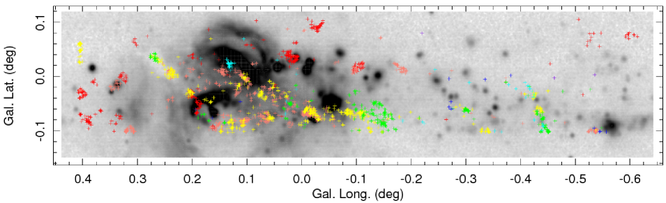
Figure 3: Reverse grayscale of the 21 micron MSX image of region surveyed with methanol masers shown as “+”. Velocity is color coded, red$>$80 km $s^{-1}$, salmon=60 km $s^{-1}$, yellow=30 km $s^{-1}$, green=0 km $s^{-1}$, cyan=-30 km $s^{-1}$, blue=-60 km $s^{-1}$, violet$<$-80 km $s^{-1}$,

Figure 3 shows the distribution of methanol masers on the 21 micron Midcourse Space Experiment (MSX) image Egan et al. (2003). While some masers are in regions of star formation, many are coincident with infrared dark clouds (IRDC) and many have no apparent association with either star forming regions or dark clouds. While these masers have a widespread distribution, Figure 3 shows them to be highly clustered with clusters having a relatively narrow range of velocities indicating that the cluster arises from a single cloud or group of clouds.

A detailed view of the region of an IRDC, “The Brick”, is given in Figure 4. This figure shows two clusters of methanol masers in prominent IR dark regions with radial velocities around 40 and 0 km s^-1. On the left side of this figure is the star forming region IRAS1743-2838 (0.33-0.02) (Avedisova, 2002) with a cluster of masers near 76 km s^-1.

We note a large number of new masers compared to the number of 36.2 GHz maser candidates found in our earlier continuum observations (Yusef-Zadeh et al., 2013). This is expected as the current data have the same sensitivity as the earlier data but 1/16 of the channel width. The narrow maser features would be reduced by a factor of $\approx$16 in the older data due to the wider ”continuum” channels. Mills et al. (2015) observe the Brick cloud (G0.253+0.016) and also find an order of magnitude more methanol masers than the number of candidate masers identified by Yusef-Zadeh et al. (2013) as well as differences in source lists. There are differences in the spatial resolution of these studies (1.6”$\times$1.5” vs. 1.8”$\times$0.7”) and in the methods in which masers were identified in Mills et al. (2015) and Yusef-Zadeh et al. (2013). Mills et al. (2015) apply the Clumpfind algorithm to identify maser sources and compare the positions of their cataloged sources with our earlier measurements and find discrepancies. In addition, the discrepancies in the identification of some masers toward this cloud in Yusef-Zadeh et al. (2013) and Mills et al. (2015) could be due to different sensitivity (30 sec. vs. 24 min on source integration) and frequency resolution (16.6 km s^-1 vs. $\sim$ 1 km s^-1). Variations in maser brightness cannot be ruled out. Yusef-Zadeh et al. (2013) reported maser candidates based on continuum observation and the maser sources needed to be confirmed with higher resolution spectral line observations. Present high resolution spectroscopic observations show maser sources. A number of sources identified in Mills et al. (2015) and Yusef-Zadeh et al. (2013) have no counterparts in our present high resolution survey. These studies indicate that the spatial resolution is critical for separating masers from quasi-thermal sources which are resolved out in the high resolution A configuraton observations.

Another Galactic center cloud that shows 36.2 GHz methanol masers is the Sgr A East molecular cloud. Sjouwerman et al. (2010) identify 10 methanol masers at the interaction site between the Sgr A East supernova remnant, the 50 km s^-1 molecular cloud and the 20 km ^-1 molecular cloud. We compared the methanol masers from Sjouwerman et al. (2010) with those listed in Table 3 and found that they agree well in both velocity and position.

3.2 1.7 GHz Continuum Results

The continuum images are strongly disturbed by the artifacts of the strong emission in the neighborhood of the Galactic center (HII regions, nonthermal arcs, filaments, etc.) which is nearly completely resolved by the high resolution of the data. However, it is possible to identify a number of small and isolated sources and these are given in Table 3. Due to the strongly variable nature of the images, it is not possible to characterize the selection criteria such as the minimum flux density.

3.3 OH (1612, 1665/7, 1720 MHz) Masers

Masers were identified in the combined spectral cubes in the manner described in Section 2.1.4 with a minimum peak flux density the greater of 8 times the local RMS and 15% of the channel peak flux density. Maser velocity and width were then determined from a moment analysis. A list of the 1612 MHz OH sources is given in Table 4 with 13 columns indicating the source name, celestial coordinates, Galactic coordinates, the flux density, the peak velocity, the line-width, spectrum type and the lower limit on the brightness temperature. The column “Type” identifies double (“D”) and single (“S”) peaked spectra. Sample spectra are shown in Figure 6. Spectra are in two distinct types, double peaked (“D”) typical of evolved stars and single peaked (“S”) with the former dominating the sample. Velocities and widths given in Table 4 for type “D” sources are those of the stronger component; the typical total velocity width is $\sim$40 km s^-1.

A list of the 1665 MHz OH sources is given in Table 5; sample spectra are shown in Figure 7. The 1667 MHz OH sources are given in Table 6 and spectra are shown in Figure 8. 1720 MHz OH sources are listed in Table 7 with spectra displayed in Figure 9.

The brightness temperature limits on the OH sources given in Tables 4–7 indicate a nonthermal, i.e. maser, origin of these sources. Most of the 1612 MHz masers have a double horned spectrum characteristic of evolved stars such as AGB stars although several are very narrow, single peaked spectrum sources. The 1665 MHz masers, as illustrated in Figure 7, have velocity structure over a range of a few to several 10’s of km $s^{-1}$. The negative features in the 1665 MHz spectra of GCA1665.09 and GCA1665.10 are due to nearby strong masers like GCA1665.12.

The few 1667 MHz masers detected have a relatively simple velocity structure with one or two components of width a few km $s^{-1}$. The 1720 MHz masers detected are all very narrow in velocity. The 1720 MHz maser GCA1720.05, is associated with a non thermal continuum source in Sgr B2(M) and is discussed in Yusef-Zadeh et al. (2016) as possibly associated with a SNR interacting with the Sgr B2 molecular cloud.

There have been numerous large scale OH surveys of the Galactic center over the last three decades. Sensitive OH observations of the inner degree of the Galactic center identified 1612 MHz masers associated with OHIR stars (Lundqvist et al. 1992, 1995; Sjowermann et al. 1998). The detection of OH(1612 MHz) masers, as listed in Table 4, have all been identified in past surveys. There have also been a large number of targeted OH surveys of the Sgr A complex and Sgr B2 at 1720 and 1665, 1667 MHz (e.g., Caswell & Haynes 1983; Gaume & Mutel 1987; Argon, Reid & Menten 2000; Yusef-Zadeh et al. 1996, 1999, 2016; Karlsson et al. 2003; Sjouwerman et al. 1998, 2002; Caswell, Green and Phillips 2013). The OH (1720 MHz) masers identified in Table 7 are concentrated in the Sgr A complex and Sgr B2, thus have been detected previously (Argon, Reid & Menten 2000; Yusef-Zadeh et al. 1999). Of the OH masers at 1665 and 1667 MHz, GCA1665.02, GCA1665.03, GCA1665.05, GCA1667.01, GCA1667.04, have not been identified in previous surveys.

Figure 1: Pointing centers of the L Band observations and locations of OH masers; large circles show the half power radius. “$\star$” = 1720 MHz, “*” = 1667 MHz, “$\circ$” = 1665 MHz, “$\times$” = 1612 MHz.

Figure 2: Pointing centers of the Ka band observations and circles showing the half power radius.

Figure 4: Closeup of the reverse grayscale of the 21 micron MSX image of an IRDC (“The Brick”) with methanol masers shown as crosses. Velocity is color coded, red$>$80 km $s^{-1}$, salmon=60 km $s^{-1}$, yellow=30 km $s^{-1}$, green=0 km $s^{-1}$, cyan=-30 km $s^{-1}$.

Figure 5: Sample methanol maser spectra, the source name is given above each plot.

Figure 6: Sample 1612 MHz OH maser spectra. The source name is given above each plot.

Figure 7: Sample 1665 MHz OH maser spectra.

Figure 8: 1667 MHz OH maser spectra

Figure 9: 1720 MHz OH maser spectra

Table 1: 36 GHz continuum Catalog

Name	RA 2000	$\pm$	Dec 2000	$\pm$	Flux	$\pm$
		′′		′′	mJy beam-1	mJy beam-1
GCA36.01	17 43 50.794	0.007	-29 22 01.72	0.009	3.44	0.39
GCA36.02	17 44 06.910	0.006	-29 24 16.42	0.006	4.62	0.24
GCA36.03	17 45 16.181	0.005	-29 03 15.43	0.006	2.83	0.22
GCA36.04	17 45 39.822	0.006	-29 00 23.52	0.008	62.78	6.46
GCA36.05	17 45 39.925	0.004	-29 00 25.00	0.009	73.21	7.17
GCA36.06	17 45 40.039	0.001	-29 00 27.92	0.001	1160.05	8.20
GCA36.07	17 45 40.094	0.006	-29 00 31.93	0.008	58.37	7.28
GCA36.08	17 45 58.318	0.001	-28 53 32.82	0.001	7.71	0.23
GCA36.09	17 46 04.468	0.006	-28 34 21.47	0.010	4.21	0.52
GCA36.10	17 46 10.536	0.001	-28 55 50.03	0.001	16.02	0.33

Table 2: Sample Detected Methanol Masers

Name	RA 2000	$\pm$	Dec 2000	$\pm$	G. long	G. lat	Flux	$\pm$	Vel	Width	TB
		′′		′′	$\circ$	$\circ$	mJy	mJy	km s-1	km s-1	105 K
GCACH3OH.0001	17 43 51.894	0.004	-29 25 16.61	0.008	-0.614	0.073	257	28	157.3	1.0	$>$ 0.34
GCACH3OH.0002	17 43 51.947	0.008	-29 24 53.59	0.013	-0.608	0.076	270	28	153.2	1.0	$>$ 0.36
GCACH3OH.0003	17 43 52.060	0.008	-29 24 49.26	0.007	-0.607	0.077	305	31	157.3	1.0	$>$ 0.41
GCACH3OH.0004	17 43 52.328	0.004	-29 24 16.16	0.006	-0.599	0.081	228	28	177.5	1.4	$>$ 0.30
GCACH3OH.0005	17 43 53.234	0.003	-29 24 18.79	0.006	-0.598	0.077	376	25	176.3	1.1	$>$ 0.50
GCACH3OH.0006	17 43 53.267	0.005	-29 24 19.24	0.007	-0.598	0.077	321	22	179.0	1.4	$>$ 0.43
GCACH3OH.0007	17 43 53.289	0.004	-29 24 15.71	0.006	-0.597	0.078	879	32	177.6	1.8	$>$ 1.17
GCACH3OH.0008	17 43 53.290	0.005	-29 24 17.05	0.009	-0.597	0.078	562	33	177.6	1.4	$>$ 0.75
GCACH3OH.0009	17 43 53.911	0.002	-29 24 10.93	0.002	-0.594	0.076	254	30	177.5	1.4	$>$ 0.34
GCACH3OH.0010	17 43 54.893	0.008	-29 24 06.48	0.012	-0.592	0.074	284	34	177.5	1.4	$>$ 0.38
GCACH3OH.0011	17 43 55.075	0.002	-29 24 34.19	0.002	-0.598	0.070	249	31	177.5	1.4	$>$ 0.33
GCACH3OH.0012	17 43 55.242	0.005	-29 24 15.75	0.009	-0.593	0.072	224	24	177.5	1.4	$>$ 0.30

Note. — Table 2 is published in its entirety in the electronic edition of the Astrophysical Journal.

A portion is shown here for guidance regarding its form and content.

Table 3: 1.7 GHz continuum Catalog

Name	RA 2000	$\pm$	Dec 2000	$\pm$	Flux	$\pm$
		′′		′′	mJy beam-1	mJy beam-1
GCA1.7.01	17 44 37.0792	0.11	-28 57 09.164	0.11	75.76	3.709
GCA1.7.02	17 45 01.4628	0.35	-29 03 35.031	0.19	26.20	2.430
GCA1.7.03	17 45 11.2478	0.20	-29 06 00.345	0.22	32.41	2.266
GCA1.7.04	17 45 11.3584	0.27	-29 05 46.326	0.21	34.41	3.068
GCA1.7.05	17 45 24.7825	0.33	-28 53 16.822	0.26	43.91	4.351
GCA1.7.06	17 45 40.0471	0.07	-29 00 27.992	0.05	649.34	18.690
GCA1.7.07	17 45 52.4887	0.06	-28 20 25.724	0.10	70.43	2.801
GCA1.7.08	17 46 05.8111	0.26	-28 49 04.330	0.31	35.05	3.442
GCA1.7.09	17 46 07.1865	0.32	-28 45 57.140	0.16	39.12	3.357
GCA1.7.10	17 46 07.2753	0.28	-28 45 52.439	0.17	28.56	2.275
GCA1.7.11	17 47 14.6736	0.14	-28 26 55.193	0.34	63.41	5.939
GCA1.7.12	17 47 14.7915	0.32	-28 26 51.494	0.20	54.11	5.271
GCA1.7.13	17 47 20.4756	0.08	-28 23 45.033	0.07	276.95	11.153

Table 4: Detected 1612 MHz OH Emission

Name	RA 2000	$\pm$	Dec 2000	$\pm$	G. long	G. lat	Flux	$\pm$	Vel	Width	Type	TB
		”		”	$\circ$	$\circ$	mJy	mJy	km s-1	km s-1		106 K
GCA1612.01	17 43 45.471	0.042	-29 26 16.80	0.06	-0.640	0.084	3520	63	-198.4	2.1	D	$>$ 0.35
GCA1612.02	17 44 06.894	0.101	-29 24 16.24	0.15	-0.571	0.036	1263	62	0.4	6.9	S?	$>$ 0.13
GCA1612.03	17 44 34.972	0.102	-29 04 35.54	0.15	-0.238	0.120	2249	107	10.0	2.4	D	$>$ 0.22
GCA1612.04	17 44 57.746	0.176	-29 20 42.14	0.27	-0.424	-0.091	613	73	-72.4	1.8	D	$>$ 0.06
GCA1612.05	17 45 31.439	0.200	-28 46 21.97	0.15	0.128	0.103	863	79	-40.6	3.1	D?	$>$ 0.09
GCA1612.06	17 45 33.502	0.109	-29 25 06.83	0.13	-0.419	-0.240	2819	120	-100.7	5.6	D	$>$ 0.28
GCA1612.07	17 45 38.620	0.194	-28 59 45.24	0.21	-0.048	-0.035	1113	98	96.8	2.8	S	$>$ 0.11
GCA1612.08	17 45 40.178	0.122	-28 59 47.49	0.15	-0.046	-0.041	2358	110	52.3	3.0	D	$>$ 0.24
GCA1612.09	17 45 40.482	0.109	-29 05 02.94	0.06	-0.120	-0.087	3946	118	-32.1	3.3	D	$>$ 0.39
GCA1612.10	17 45 46.432	0.111	-29 01 46.04	0.08	-0.062	-0.077	3285	107	-71.2	5.7	D	$>$ 0.33
GCA1612.11	17 45 49.416	0.246	-28 58 48.76	0.18	-0.014	-0.061	815	89	33.8	3.8	D	$>$ 0.08
GCA1612.12	17 45 51.916	0.203	-28 44 51.18	0.22	0.189	0.052	799	80	-8.3	2.1	D?	$>$ 0.08
GCA1612.13	17 45 54.208	0.162	-28 31 46.99	0.16	0.379	0.159	1112	77	126.1	3.3	D	$>$ 0.11
GCA1612.14	17 45 55.828	0.093	-28 45 18.24	0.12	0.190	0.036	2442	96	148.2	5.9	D	$>$ 0.24
GCA1612.15	17 46 19.130	0.121	-28 31 57.12	0.21	0.424	0.079	783	72	-21.4	3.3	D	$>$ 0.08
GCA1612.16	17 46 22.109	0.125	-28 46 22.81	0.21	0.225	-0.055	951	87	-88.6	0.9	D	$>$ 0.10
GCA1612.17	17 46 32.135	0.061	-28 41 04.16	0.09	0.319	-0.040	3128	85	92.6	4.5	D	$>$ 0.31
GCA1612.18	17 46 35.339	0.170	-28 58 57.19	0.16	0.071	-0.205	1517	112	127.2	2.4	D	$>$ 0.15
GCA1612.19	17 46 39.039	0.161	-28 28 06.75	0.10	0.517	0.050	980	69	185.3	1.4	D	$>$ 0.10
GCA1612.20	17 47 18.646	0.135	-28 22 54.14	0.19	0.666	-0.029	1349	83	72.2	2.3	D	$>$ 0.13
GCA1612.21	17 47 20.146	0.211	-28 23 05.10	0.13	0.667	-0.035	1657	97	65.2	8.9	D	$>$ 0.17
GCA1612.22	17 47 25.062	0.112	-28 36 33.31	0.16	0.484	-0.167	1529	77	153.4	3.6	D	$>$ 0.15
GCA1612.23	17 47 25.434	0.044	-28 23 36.38	0.06	0.669	-0.056	3363	92	68.4	1.2	S	$>$ 0.34

Table 5: Detected 1665 MHz OH Emission

Name	RA 2000	$\pm$	Dec 2000	$\pm$	G. long	G. lat	Flux	$\pm$	Vel	Width	TB
		′′		′′	$\circ$	$\circ$	mJy	mJy	km s-1	km s-1	106 K
GCA1665.01	17 44 40.572	0.027	-29 28 15.37	0.051	-0.564	-0.103	2957	54	-50.9	0.9	$>$ 0.30
GCA1665.02	17 45 39.085	0.064	-29 23 29.71	0.096	-0.385	-0.243	2282	71	21.8	3.9	$>$ 0.23
GCA1665.03	17 46 21.399	0.014	-28 35 38.99	0.026	0.376	0.040	6386	61	37.0	2.9	$>$ 0.64
GCA1665.04	17 46 28.696	0.156	-29 20 29.25	0.228	-0.249	-0.371	565	61	-6.7	0.7	$>$ 0.06
GCA1665.05	17 46 37.438	0.122	-28 37 29.91	0.398	0.380	-0.026	3760	448	68.5	0.7	$>$ 0.38
GCA1665.06	17 47 09.121	0.091	-28 46 15.82	0.145	0.315	-0.201	913	46	27.0	2.1	$>$ 0.09
GCA1665.07	17 47 19.908	0.051	-28 22 16.05	0.070	0.678	-0.027	4228	234	70.5	1.5	$>$ 0.42
GCA1665.08	17 47 20.000	0.131	-28 22 55.73	0.275	0.669	-0.033	589	50	84.3	0.9	$>$ 0.06
GCA1665.09	17 47 20.042	0.033	-28 22 40.75	0.063	0.672	-0.031	4139	94	55.2	2.4	$>$ 0.41
GCA1665.10	17 47 20.048	0.048	-28 23 46.24	0.118	0.657	-0.041	1733	59	49.6	2.1	$>$ 0.17
GCA1665.11	17 47 20.107	0.037	-28 23 05.12	0.040	0.667	-0.035	17827	201	61.6	2.5	$>$ 1.78
GCA1665.12	17 47 20.476	0.013	-28 23 45.00	0.023	0.658	-0.042	143454	1236	69.0	1.9	$>$14.33
GCA1665.13	17 47 45.067	0.014	-28 44 28.08	0.017	0.409	-0.298	1154	85	68.5	0.9	$>$ 0.12
GCA1665.14	17 47 47.351	0.023	-28 44 31.76	0.105	0.412	-0.305	471	54	69.4	1.7	$>$ 0.05

Table 6: Detected 1667 MHz OH Emission

Name	RA 2000	$\pm$	Dec 2000	$\pm$	G. long	G. lat	Flux	$\pm$	Vel	Width	TB
		′′		′′	$\circ$	$\circ$	mJy	mJy	km s-1	km s-1	106 K
GCA1667.01	17 44 51.304	0.081	-29 24 54.56	0.097	-0.496	-0.107	418	37	-61.8	0.9	$>$ 0.04
GCA1667.02	17 45 33.515	0.107	-29 25 06.92	0.170	-0.419	-0.240	507	47	-71.0	1.7	$>$ 0.05
GCA1667.03	17 45 38.605	0.077	-28 59 45.26	0.077	-0.048	-0.035	429	50	69.4	0.9	$>$ 0.04
GCA1667.04	17 46 15.345	0.064	-28 48 47.75	0.117	0.177	-0.055	505	33	-19.0	0.9	$>$ 0.05
GCA1667.05	17 47 20.402	0.508	-28 23 03.88	0.166	0.667	-0.036	893	99	53.3	1.7	$>$ 0.09

Table 7: Detected 1720 MHz OH Emission

Name	RA 2000	$\pm$	Dec 2000	$\pm$	G. long	G. lat	Flux	$\pm$	Vel	Width	TB
		′′		′′	$\circ$	$\circ$	mJy	mJy	km s-1	km s-1	106 K
GCA1720.01	17 45 38.800	0.106	-28 59 42.57	0.169	-0.047	-0.036	765	57	44.3	0.9	$>$ 0.08
GCA1720.02	17 45 40.605	0.171	-28 59 44.32	0.095	-0.044	-0.042	1303	61	133.1	1.0	$>$ 0.13
GCA1720.03	17 45 43.471	0.131	-29 01 31.80	0.237	-0.064	-0.066	443	45	58.4	0.8	$>$ 0.04
GCA1720.04	17 45 44.335	0.055	-29 01 18.98	0.031	-0.060	-0.067	4508	68	67.2	1.3	$>$ 0.45
GCA1720.05	17 47 20.029	0.148	-28 23 12.15	0.220	0.665	-0.036	748	74	62.3	0.7	$>$ 0.07

References

- Argon et al. (2000) Argon, A. L., Reid, M. J., & Menten, K. M. 2000, ApJS, 129, 159
- Avedisova (2002) Avedisova, V. S., 2002, ARep, 46, 193.
- Bally et al. (1988) Bally, J., Stark, A. A., Wilson, R. W., & Henkel, C. 1988, ApJ, 324, 223
- Caswell & Haynes (1983) Caswell, J. L., & Haynes, R. F. 1983, Australian Journal of Physics, 36, 361
- Caswell et al. (2013) Caswell, J. L., Green, J. A., & Phillips, C. J. 2013, MNRAS, 431, 1180
- Condon (1997) Condon, J. J. 1997, PASP, 109, 166
- Cotton (2008) Cotton, W. D. 2008, PASP, 120, 439
- Dahmen et al. (1997) Dahmen, G., Huettemeister, S., Wilson, T. L., et al. 1997, A&AS, 126
- Egan et al. (2003) Egan, M. P., Price, S. D., Kramer, K. E., et al. 2003, Air Force Research Laboratory Technical Report AFRL-VS-TR-2003-1589
- Frail et al. (1994) Frail, D. A., Goss, W. M., & Slysh, V. I. 1994, ApJ, 424, L111
- Gaume & Mutel (1987) Gaume, R. A., & Mutel, R. L. 1987, ApJS, 65, 193
- Hewitt et al. (2008) Hewitt, J. W., Yusef-Zadeh, F., & Wardle, M. 2008, ApJ, 683, 189
- Huettemeister et al. (1993) Huettemeister, S., Wilson, T. L., Bania, T. M., & Martin-Pintado, J. 1993, A&A, 280, 255
- Karlsson et al. (2003) Karlsson, R., Sjouwerman, L. O., Sandqvist, A., & Whiteoak, J. B. 2003, A&A, 403, 1011
- LaRosa et al. (2005) LaRosa, T. N., Brogan, C. L., Shore, S. N., et al. 2005, ApJ, 626, L23
- Lindqvist et al. (1992) Lindqvist, M., Habing, H. J., & Winnberg, A. 1992, A&A, 259, 118
- Lindqvist et al. (1992) Lindqvist, M., Winnberg, A., Habing, H. J., & Matthews, H. E. 1992, A&AS, 92, 43
- Jones et al. (2012) Jones, P. A., Burton, M. G., Cunningham, M. R., et al. 2012, MNRAS, 419, 2961
- Mehringer & Menten (1997) Mehringer, D. M., & Menten, K. M. 1997, ApJ, 474, 346
- Mills et al. (2015) Mills, E. A. C., Butterfield, N., Ludovici, D. A., et al. 2015, ApJ, 805, 72
- Oka et al. (1998) Oka, T., Hasegawa, T., Sato, F., Tsuboi, M., & Miyazaki, A. 1998, ApJS, 118, 455
- Oka et al. (2005) Oka, T., Geballe, T. R.,G oto, M., Usuda, T., & McCall, B. J. 2005, ApJ, 632, 882
- Roberts et al. (2007) Roberts, J. F., Rawlings, J. M. C., Viti, S., & Williams, D. A. 2007, MNRAS, 382, 733
- Sjouwerman et al. (1998) Sjouwerman, L. O., van Langevelde, H. J., Winnberg, A., & Habing, H. J. 1998, A&AS, 128, 35
- Sjouwerman et al. (2002) Sjouwerman, L. O., Lindqvist, M., van Langevelde, H. J., & Diamond, P. J. 2002, A&A, 391, 967
- Sjouwerman et al. (2010) Sjouwerman, L. O., Pihlström, Y, M. and Fish, V. L. 2010, ApJ 710, L111
- Tsuboi et al. (1999) Tsuboi, M., Handa, T., & Ukita, N. 1999, ApJS, 120, 1
- Voronkov et al. (2006) Voronkov, M. A., Brooks, K. J., Sobolev, A. M. et al. 2006, MNRAS, 373, 411
- Wardle (1999) Wardle, M. 1999, ApJ, 525, L101
- Yusef-Zadeh et al. (1996) Yusef-Zadeh, F., Roberts, D. A., Goss, W. M., Frail, D. A., & Green, A. J. 1996, ApJ, 466, L25
- Yusef-Zadeh et al. (1999) Yusef-Zadeh, F., Roberts, D. A., Goss, W. M., Frail, D. A., & Green, A. J. 1999, ApJ, 512, 230
- Yusef-Zadeh et al. (2013) Yusef-Zadeh, F., Cotton, W., Viti, S., Wardle, M., Royster, M. 2013 ApJ, 764, L19
- Yusef-Zadeh et al. (2007) Yusef-Zadeh, F., Wardle, M., & Roy, S. 2007, ApJ, 665, L123
- Yusef-Zadeh et al. (2013) Yusef-Zadeh, F., Wardle, M., Lis, D., et al. 2013, Journal of Physical Chemistry A, 117, 9404
- Yusef-Zadeh et al. (2016) Yusef-Zadeh, F. Cotton, W.,Wardle, M., Intema, H. 2016 ApJ, 819, L35