Spatially modulated instabilities of holographic gauge-gravitational anomaly

Abstract

We performed a study of the perturbative instabilities in Einstein-Maxwell-Chern-Simons theory with a gravitational Chern-Simons term, which is dual to a strongly coupled field theory with both chiral and mixed gauge-gravitational anomaly. With an analysis of the fluctuations in the near horizon regime at zero temperature, we found that there might be two possible sources of instabilities. The first one corresponds to a real mass-squared which is below the BF bound of AdS₂, and it leads to the bell-curve phase diagram at finite temperature. The effect of mixed gauge-gravitational anomaly is emphasised. Another source of instability is independent of gauge Chern-Simons coupling and exists for any finite gravitational Chern-Simons coupling. There is a singular momentum close to which unstable mode appears. The possible implications of this singular momentum are discussed. Our analysis suggests that the theory with a gravitational Chern-Simons term around Reissner-Nordström black hole is unreliable unless the gravitational Chern-Simons coupling is treated as a small perturbative parameter.

1 Introduction

It is well known that there is a novel spatially modulated instability for AdS Reissner-Nordström (RN) black hole in five dimensional Einstein-Maxwell theory with a Chern-Simons term Nakamura:2009tf ; Ooguri:2010kt ; Donos:2012wi . More precisely, for a large enough Chern-Simons coupling constant, below some critical temperature the translational invariance in one of the spatial directions of RN black hole is spontaneously broken and a spatially modulated black hole with helical current is the preferred state. From the perspective of gauge/gravity duality Zaanen:2015oix , one concludes that the dual field theory, namely a four dimensional strongly coupled chiral anomalous system, suffers from spatially modulated instability. Thus this holographic model may provide interesting dual descriptions of systems in nature, and clarify several aspects of their phase structures, including quark-gluon plasma and Weyl/Dirac (semi-)metals.

On the other hand, in a four dimensional chiral field theory system, besides pure gauge anomalies, there is another type of anomaly, the mixed gauge-gravitational anomaly, which is the gravitational contribution to the chiral anomaly (see e.g. AlvarezGaume:1983ig ). These two types of anomaly are distinguished depending on the three insertions in the triangle diagram being of spin one, or an insertion of spin one and the other two being of spin two. For an anomalous system at finite temperature and chemical potential, the dynamics of anomaly enters into the energy-momentum conservation and current conservation equations and will contribute to anomaly-induced transports Son:2009tf ; Jensen:2012kj . Remarkably, the mixed gauge-gravitational anomaly leads to important observable effects in many body physics at finite temperature including e.g. chiral vortical effect Landsteiner:2011cp , odd (Hall) viscosity Landsteiner:2016stv and negative thermal magnetoresistivity Lucas:2016omy .

However, so far a study on possible effects of spatially modulated instability due to the mixed gauge-gravitational anomaly is missing. In the holographic context the mixed gauge-gravitational anomaly is encoded in gravity via a gravitational Chern-Simons term Landsteiner:2011iq . Unlike the pure gauge Chern-Simons term, the gravitational one is higher order in derivatives endowing the theory with the subtleties of higher derivative gravity, we will come back to this point in section 2. Our aim is to explore the possible instability due to the mixed gauge-gravitational anomaly of an anomalous system. Our strategy to study the instability is by analysing the fluctuation around Reissner-Nordström black hole solution to examine the possible unstable modes.

At zero temperature we studied the fluctuations around the near horizon geometry AdS₂ $\times$ R³ and analyse the instabilities. From the AdS₂ point of view, we found two sources of instabilities. One is the Breitenlohner-Freedman (BF) bound violation which is essentially the same as the case without mixed gauge-gravitational anomaly. Another one is related to a degenerate point in the equations, which is characterized by a momentum that we will call singular momentum. At finite temperature the first source of instability plays as a sufficient condition for the bell-curve phase diagram. The second source of instability exists at any finite gravitational Chern-Simons coupling. There always exists a mode with BF bound violation close to the singular momentum, and we could expect the existence of a spontaneous symmetry breaking solution. We will discuss the implications of this singular momentum for finite temperature in section 3.2.1.

The rest of the paper is organised as follows. In section 2 we outline the setup of gravitational theory and fix the conventions of the paper. In section 3 we study the perturbative instabilities for the RN black hole on the gravity side to construct the phase diagram as well as discuss possible physical implications of a singular momentum. We conclude in section 4 with a summary of results and a list of open questions.

2 Setup

Let us first briefly review the basic setup for the holographic systems encoding both the gauge and mixed gauge-gravitational anomaly in the dual field theory Landsteiner:2011iq . The minimal setup of five dimensional gravitational action we consider is

$$\mathcal{S} = \frac{1}{2\kappa^{2}}\int d^{5}x\sqrt{-g}\bigg{[}R+\frac{12}{L^{2}}-\frac{L^{2}}{4}F^{2}+\epsilon^{\mu\nu\rho\sigma\tau}A_{\mu}\Big{(}\frac{\alpha L^{3}}{3}F_{\nu\rho}F_{\sigma\tau}+\lambda L^{3}R^{\beta}_{~{}\delta\nu\rho}R^{\delta}_{~{}\beta\sigma\tau}\Big{)}\bigg{]}~{}~{}~{}~{}~{}~{}$$ (2.1)

where $2\kappa^{2}$ is five-dimentional gravitational coupling constant, $L$ is the AdS radius and $F_{\mu\nu}=\partial_{\mu}A_{\nu}-\partial_{\nu}A_{\mu}$ is the gauge field strength. In the following we will set $2\kappa^{2}=L=1$. Note that $\alpha$ and $\lambda$ are dimensionless quantity.

The equations of motion for this system are

$$R_{\mu\nu}-\frac{1}{2}g_{\mu\nu}\Big{(}R+12-\frac{1}{4}F^{2}\Big{)}-\frac{1}{2}F_{\mu\rho}F_{\nu}^{~{}\rho}-2\lambda\epsilon_{\alpha\beta\rho\tau(\mu|}\nabla_{\delta}(F^{\beta\alpha}R^{\delta~{}~{}\rho\tau}_{~{}|\nu)}) = 0\,,$$ (2.2)

$$\nabla_{\nu}F^{\nu\mu}+\epsilon^{\mu\tau\beta\rho\sigma}\Big{[}\alpha F_{\tau\beta}F_{\rho\sigma}+\lambda R^{\delta}_{~{}\xi\tau\beta}R^{\xi}_{~{}\delta\rho\sigma}\Big{]} = 0\,,$$ (2.3)

where $A_{(\mu}B_{\nu)}=\frac{1}{2}(A_{\mu}B_{\nu}+A_{\nu}B_{\mu}).$

The Reissner-Nordström black brane is a solution of the system

$$ds^{2}=-Udt^{2}+\frac{dr^{2}}{U}+r^{2}(dx^{2}+dy^{2}+dz^{2})\,,~{}~{}A=\phi dt$$ (2.4)

where

$$U=r^{2}-\frac{r_{+}^{4}}{r^{2}}+\frac{\mu^{2}}{3}\bigg{(}\frac{r_{+}^{4}}{r^{4}}-\frac{r_{+}^{2}}{r^{2}}\bigg{)}\,,~{}~{}~{}\phi=\mu\Big{(}1-\frac{r_{+}^{2}}{r^{2}}\Big{)}\,.$$ (2.5)

From the AdS/CFT correspondence Zaanen:2015oix , the isotropic dual field theory lives at the conformal boundary $r\to\infty$ with the temperature

$$T=\frac{U^{\prime}(r_{+})}{4\pi}=\frac{r_{+}}{\pi}-\frac{\mu^{2}}{6\pi r_{+}}$$ (2.6)

and a finite (axial) chemical potential $\mu$. The Chern-Simons terms do not contribute to the thermodynamical quantities for Reissner-Nordström black brane. The pure gauge anomaly and mixed gauge-gravitational anomaly of this system are fixed by $\alpha$ and $\lambda$ respectively Landsteiner:2011iq . More precisely, the dual field theory describes a chiral fluid with an anomalous axial U(1) symmetry whose conservation equations in terms of covariant currents are

$$\nabla_{a}T^{ab} = F^{ba}J_{a}-2\lambda\nabla_{b}(\varepsilon^{cefl}F_{ce}R^{ba}_{~{}~{}fl})\,,$$ (2.7)

$$\nabla_{a}J^{a} = -\big{(}\alpha\varepsilon_{abcd}F^{ab}F^{cd}+\lambda\varepsilon^{abcd}R^{e}_{~{}fab}R^{f}_{~{}ecd}\big{)}\,.$$ (2.8)

In the context of the low energy effective field theory, other higher derivative terms should, in principle, be included in theory (2.1) and the four-derivatives terms should be treated as perturbative corrections. However, the particular theory (2.1), which is considered from a bottom-up holographic point of view has the advantage of being the minimal model from which the dual (non)-conservation equations precisely match the ones of chiral fluid. Therefore, to capture the physical effects due to the anomalies, including anomaly-induced transport and phase transitions, (2.1) is sufficient for simplicity.

There are reasons to treat the four-derivatives term non-perturbatively. In the pure AdS₅ case, the mixed anomaly term does not contribute to the linear fluctuations of the theory (2.1), and no ghost will appear, this means that one could treat $\lambda$ as an arbitrary constant. In the Schwartzschild black hole case, as we shown in the appendix A from the perspective of quasi-normal modes, no unstable modes seems to appear when treating $\lambda$ as an order one number. Moreover, for a single Weyl fermion, we have $\alpha\sim\lambda\sim\mathcal{O}(1)$, i.e. the mixed gravitational anomaly has the same importance of the chiral anomaly, and we remind the reader our motivation is purely phenomenological. From these perspectives, it is tempting to treat $\lambda$ as a non-perturbative parameter although in general the higher derivative terms might have potential causality issues Camanho:2014apa , and suffer of Ostrogradsky’s instabilities.

In the following, we shall study the effects due to “non-perturbative” gravitational Chern-Simons coupling on the stability of Reissner-Nordström black hole.

3 Perturbative instability at zero and finite temperature

In this section, we will study the perturbative instability of the gravitational system at zero and finite temperature respectively. The effect of the mixed gauge-gravitational anomaly on the instability will be explored.

3.1 Instability at zero temperature

In this subsection we will study the stability of the extremal RN black hole solution in the gravitational theory (2.1).

At zero temperature, i.e. extremal RN ($r_{+}=\mu/\sqrt{6}$), the near horizon geometry of RN black hole is AdS₂ $\times$ R³

$$ds^{2}=\frac{1}{12\rho^{2}}(-dt^{2}+d\rho^{2})+(dx^{2}+dy^{2}+dz^{2})\,,~{}~{}~{}A_{t}=\frac{1}{\sqrt{6}\rho}\,.$$ (3.9)

and the BF bound for the scalar mass squared in AdS₂ is $-3.$

Following Nakamura:2009tf , we consider fluctuations around the near horizon geometry (3.9)

$$\delta g_{ai}=h_{ai}(t,\rho)e^{ikx}\,,~{}~{}~{}\delta A_{i}=a_{i}(t,\rho)e^{ikx}$$ (3.10)

with $i\in\{y,z\}$ and $a\in\{t,x\}$ around the near horizon geometry (3.9). By plugging these fluctuations into the equations of motion (2.2, 2.3), we find that the equations from gravity sector are

$$-6\rho^{2}h_{ti}^{\prime\prime}-12\rho h_{ti}^{\prime}+\frac{k^{2}}{2}h_{ti}+\frac{ik}{2}\partial_{t}h_{xi}+\sqrt{6}a_{i}^{\prime}~{}~{}~{}~{}~{}~{}~{}$$

$$+i4\sqrt{6}k\lambda\epsilon^{ij}\big{(}12\rho^{2}h_{tj}^{\prime\prime}+24\rho h_{tj}^{\prime}-k^{2}h_{tj}-ik\partial_{t}h_{xj}+2\sqrt{6}a_{j}^{\prime}\big{)} = 0\,,$$ (3.11)

$$h_{xi}^{\prime\prime}-\partial_{t}^{2}h_{xi}+ik\partial_{t}h_{ti}-i8\sqrt{6}k\lambda\epsilon^{ij}\big{(}h_{xj}^{\prime\prime}-\partial_{t}^{2}h_{xj}+ik\partial_{t}h_{tj}\big{)} = 0\,,$$ (3.12)

$$\sqrt{6}i\partial_{t}a_{i}-6i\rho^{2}\partial_{t}h_{ti}^{\prime}-\frac{k}{2}h_{xi}^{\prime}+i4\sqrt{6}k\lambda\epsilon^{ij}\big{(}kh_{xj}^{\prime}+12i\rho^{2}\partial_{t}h_{tj}+2\sqrt{6}i\partial_{t}a_{j}\big{)} = 0$$ (3.13)

where the prime ^′ is the derivative with respect to $\rho$ and $\epsilon^{yz}=-\epsilon^{zy}=1$. Note that only two of them are independant since $-i\partial_{t}(\ref{eq:g1})+\frac{k}{2}(\ref{eq:g2})+\partial_{\rho}(\ref{eq:g3})=0$. Thus we shall focus on (3.11) and (3.13). The equation from gauge sector is

$$12\rho^{2}(a_{i}^{\prime\prime}-\partial_{t}^{2}a_{i})-k^{2}a_{i}-24\sqrt{6}\rho^{2}\big{(}h_{ti}^{\prime}+8\sqrt{6}ik\lambda\epsilon^{ij}h_{tj}^{\prime}\big{)}-16\sqrt{6}ik\alpha\epsilon^{ij}a_{j}=0\,.$$ (3.14)

Via the sequence of field redefinitions

$$\varphi_{i} = a_{i}+i8\sqrt{6}k\lambda\epsilon^{ij}a_{j}-\sqrt{6}\rho^{2}\big{(}h_{ti}^{\prime}-i8\sqrt{6}k\lambda\epsilon^{ij}h_{tj}^{\prime}\big{)}\,,$$ (3.15)

$$\Phi_{a} = (a_{y}+ia_{z},a_{y}-ia_{z},\varphi_{y}+i\varphi_{z},\varphi_{y}-i\varphi_{z})\,,$$ (3.16)

(3.13) can be rewritten as two first order PDEs

$$\partial_{t}\Phi_{a}+4ik\left((-1)^{a}k\lambda+\frac{1}{8\sqrt{6}}\right)\left(h^{\prime}_{xy}-i(-1)^{a}h^{\prime}_{xz}\right)=0\,,\quad a=3,4$$ (3.17)

from which we know that in general the dynamics of $h_{xi}$ is totally determined by $\Phi_{3,4}.$

The redefinition (3.16) has a special point $k=\pm k_{s}$ with

$$k_{s}=\frac{1}{8\sqrt{6}\lambda}\,,$$ (3.18)

such that the four new redefined fields are not independent. At this specific value redefinition (3.16) reduces to

$$\Phi_{3}=2\Phi_{1}\quad\text{for}\quad k=k_{s}\,,\text{~{}~{}~{}(or~{}~{}}\Phi_{4}=2\Phi_{2}\quad\text{for}\quad k=-k_{s})\,.$$ (3.19)

We will refer to it as the singular momentum, for reasons that will be clarified below.

In order to study the possibility of violating the BF bound, we will analyze first the system at the singular momentum, and then at arbitrary values of $k$. From (3.17) we have $\partial_{t}\Phi_{3}=0$ or $\partial_{t}\Phi_{4}=0$ respectively. The equations for the independent dynamical fields are

$$\Box_{\text{AdS}_{2}}\Phi_{4,3}-\frac{1}{384\lambda^{2}}\Phi_{4,3} = 0\,,$$ (3.20)

$$\Box_{\text{AdS}_{2}}\Phi_{2,1}-\left(\frac{1}{384\lambda^{2}}-\frac{2\alpha}{\lambda}\right)\Phi_{2,1} = 0\,,$$ (3.21)

where $\Box_{\text{AdS}_{2}}=12\rho^{2}(-\partial_{t}^{2}+\partial_{\rho}^{2})$. The other two dependent (nondynamical) degrees of freedom are determined via the relations

$$\Phi_{1,2}^{\prime}=\partial_{t}\Phi_{1,2} = 0\,,$$ (3.22)

$$48\sqrt{6}\rho^{2}h_{t\pm}^{\prime}+\left(\frac{2\alpha}{\lambda}+\frac{1}{384\lambda^{2}}\right)\Phi_{1,2} = 0\,,$$ (3.23)

with $h_{t\pm}=h_{ty}\pm ih_{tz}$.

Thus we only have two dynamical field $\Phi_{4,3}$ and $\Phi_{2,1}$ at this singular momentum. Furthermore, we observe that the system is automatically diagonal in these dynamical variables, and more important is the fact the $\Phi_{4,3}$ has a positive mass, therefore always above the BF bound, however the field $\Phi_{2,1}$ has a mass that can be negative depending on the values of $(\alpha,\lambda)$. The region of instability is given by the inequality

$$|\alpha|>\Big{|}\frac{3\lambda}{2}+\frac{1}{768\lambda}\Big{|}\quad\textrm{and}\quad\alpha\lambda>0\,.$$ (3.24)

Thus exactly at the singular momentum there is no instability if $|\alpha|<\frac{1}{8\sqrt{2}}.$

Now we will discus the case $k\neq\pm k_{s}$, in this case we recover the original four degrees of freedom and the equations they satisfy read

$$(\Box_{\text{AdS}_{2}}-\mathbb{M}_{\pm}^{2}){\bf\Phi}_{\pm}=0\,,$$ (3.25)

with ${\bf\Phi}_{+}=\left(\begin{array}[]{c}\Phi_{1}\\ \Phi_{3}\\ \end{array}\right)$, ${\bf\Phi}_{-}=\left(\begin{array}[]{c}\Phi_{2}\\ \Phi_{4}\\ \end{array}\right)$ and

$$\mathbb{M}_{\pm}^{2}=\left(\begin{array}[]{cc}k^{2}-72\pm 16\sqrt{6}k(\alpha-12\lambda)+\frac{96}{1\mp 8\sqrt{6}k\lambda}&24\left(1-\frac{2}{1\mp 8\sqrt{6}k\lambda}\right)\\ -k^{2}\left(1\pm 8\sqrt{6}k\lambda\right)&k^{2}\\ \end{array}\right)\,.$$ (3.28)

For generic $\alpha$ and $\lambda$, the eigenvalues are

$$m_{j\pm}^{2} = k^{2}-36\pm 8\sqrt{6}k(\alpha-12\lambda)+\frac{48k_{s}}{k_{s}\mp k}+$$

$$(-1)^{j}\sqrt{\bigg{(}-36\pm 8\sqrt{6}k(\alpha-12\lambda)+\frac{48k_{s}}{k_{s}\mp k}\bigg{)}^{2}+24\frac{k^{2}}{k_{s}}\frac{(k_{s}\pm k)^{2}}{k_{s}\mp k}}$$

with $j=1,2.$

There is a lot of information in the above formulae:

• In absence of the anomaly, i.e. $\alpha=\lambda=0$, we have ${m_{j}^{2}}_{+}={m_{j}^{2}}_{-}$ ($j=1,2$) and $\text{min}(m_{1}^{2},m_{2}^{2})=24-2\sqrt{6}$ which is above the BF bound of (3.9). This is the well-known fact that there is no spatially modulated instability for RN black hole in Einstein-Maxwell theory.

• For $\lambda=0$, we only have gauge anomaly and we have

  $$m_{j\pm}^{2}=k^{2}+12\pm 8\sqrt{6}k\alpha+(-1)^{j}2\sqrt{6}\sqrt{k^{2}+(\sqrt{6}\pm 4\alpha k)^{2}}\,,$$ (3.30)

  which violate the BF bound when $|\alpha|>\alpha_{c}\approx 0.1448$ as studied for the first time in Nakamura:2009tf . For $\alpha=\alpha_{c}$, the minimal value of mass square is at $k_{v}/\mu\approx 1.5349$. Thus it indicates a spatially modulated phase transition.

• When $k\to k_{s}$ (or $k\to-k_{s}$), either $m_{1+}^{2}$ or $m_{2+}^{2}$ (or $m_{1-}^{2}$ or $m_{2-}^{2}$ ) become negative/positive infinity while the other mass squares coincide with (3.20, 3.21). This is due to the degenerate definition of fields at $k=\pm k_{s}$ in (3.16) which leads to (3.19). Because of this artificial infinity in (3.1), we called $k_{s}$ singular momentum. Nevertheless, when $k\neq\pm k_{s}$, (3.1) applies. Thus we conclude that close to $\pm k_{s}$ BF bound is always violated and it is a source of instability in the system.

• $m_{j}^{2}$ is invariant under $(k,\alpha,\lambda)\to-(k,\alpha,\lambda)$. This means that in order to study the unstable modes in momentum space, we can simply focus on the case with one of the $k,\alpha,\lambda$ parameter space to be positive.

• The square root in (3.1) can become complex and this is totally different from the case without the mixed gauge-gravitational anomaly Nakamura:2009tf , if that happens the system will be unstable because the unitarity condition $m_{j}^{2}>m_{\text{BF}}^{2}$ will not be satisfied. We label the critical momentum beyond which the square root become complex as $k_{*}$. Note that $k_{*}$ is a function of $\alpha$ and $\lambda$ and it can be obtained by solving the equation

  $$\bigg{(}-36+8\sqrt{6}k_{*}(\alpha-12\lambda)+\frac{48k_{s}}{k_{s}-k_{*}}\bigg{)}^{2}+24\frac{k_{*}^{2}}{k_{s}}\frac{(k_{s}+k_{*})^{2}}{k_{s}-k_{*}}=0\,.$$ (3.31)

  If $k_{*}(\alpha,\lambda)$ is the solution for $m_{j+}^{2}$, $k_{*}(-\alpha,-\lambda)$ will be for $m_{j-}^{2}$. The number of solutions for $k_{*}$ of (3.31) depend on $\alpha$ and $\lambda$. There are two situations. One could have a unique solution $k_{*}$ and for $k_{*}<k$ the mass square become complex. Another case is that one may have three solutions $k_{*1}<k_{*2}<k_{*3}$. For $k_{*1}<k<k_{*2}$ or $k_{*3}<k$, the mass square is complex while for $k_{*2}<k<k_{*3}$ the mass square is real. We label the smallest $k_{*1}$ as $k_{*}$. It can be proved that

  $$k_{s}<|k_{*}|$$ (3.32)

  independent of the value of $\alpha$.

  It is more apparent to see the above statements in the limit $k\to\infty$, we have

  $$m_{j\pm}^{2}=k^{2}+(-1)^{j}8(54)^{1/4}\sqrt{\mp\lambda}k^{3/2}+\dots,~{}~{}~{}(j=1,2)\,,$$ (3.33)

  thus one of the mass square becomes complex when $\lambda\neq 0$. This indicates that for a non-zero value of the mixed anomaly coupling $\lambda$ and arbitrary value of Chern-Simons coupling $\alpha$, the theory should be unstable around RN black hole.

• For $\alpha=0$, the complex mass momentum $k_{*}$ can be solved to be

  $$\pm 3k_{s}k_{*} = 6+k_{s}^{2}+\frac{\left(k_{s}^{4}+48k_{s}^{2}+36\right)}{\left(\left(k_{s}^{4}+153k_{s}^{2}+432+9k_{s}\sqrt{2k_{s}^{4}+213k_{s}^{2}+144}\right)k_{s}^{2}+216\right)^{1/3}}+$$ (3.34)

  $$\left(\left(k_{s}^{4}+153k_{s}^{2}+432+9k_{s}\sqrt{2k_{s}^{4}+213k_{s}^{2}+144}\right)k_{s}^{2}+216\right)^{1/3}\,.$$

  This complicated function has a simple behaviour in the two following limits

  $$k_{*} = \pm 6k_{s}^{-1}\,,\quad k_{s}\to 0~{}~{}~{}~{}(\text{or~{}}\lambda\to\infty)$$ (3.35)

  $$k_{*} = \pm k_{s}\,,~{}~{}~{}\quad k_{s}\to\infty~{}~{}~{}(\text{or~{}}\lambda\to 0)\,.$$ (3.36)

  For generic $\alpha$, we show a numerical loglogplot in Fig. 1 and one observe that when $k_{s}\to 0$ or $k_{s}\to\infty$ we have the similar behaviour as the case $\alpha=0.$

  

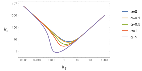
  Figure 1: The loglogplot of $k_{*}$ as a function of $k_{s}$ at different values of $\alpha$. The behaviour of $k_{*}$ at small $k_{s}$ or large $k_{s}$ is independent of $\alpha$. Note that one can always find a solution of $k_{*}$ at arbitrary $\alpha,\lambda$ and this means that the instability always exists whenever $\lambda\neq 0.$

• When $|k|<|k_{*}|$, the mass squares in (3.1) are real. We have $m_{1}^{2}<m_{2}^{2}$ and we can focus on the $m_{1}^{2}$ sector to explore the instability. For fixed $\alpha$ and $\lambda$, violating the BF bound (i.e. $\text{min}\{m_{j\pm}^{2}\}<-3$) will give a finite regime of $k$ in which there is an instability which is a generalisation of Nakamura:2009tf . After minimising (3.1) with respect to momentum, we obtain the location of the minima $k_{\textrm{min}}(\alpha,\lambda)$ as a function of the Chern-Simons couplings, plugin back this function into the mass function (3.1) and equating to the BF bound we obtain one of the Chern-Simons coupling in terms of the other, this function determines the critical values of the Chern-Simons couplings. In Fig. 2 we show the dependance of the critical Chern-Simons coupling $\alpha_{c}$ as a function of $\lambda$. For fixing $\lambda$, when $\alpha>\alpha_{c}$ the BF bound is violated. Interestingly, we found with finite $\lambda$, the critical $\alpha$ could be smaller than the gauged SUGRA bound in which $\alpha=1/(4\sqrt{3})\simeq 0.1443...>{\alpha_{c}}_{\text{min}}$. However, the complete action for SUGRA up to this order involves other higher derivative terms Cremonini:2008tw , it would be interesting to study the spatially modulated instability in the SUGRA.

  

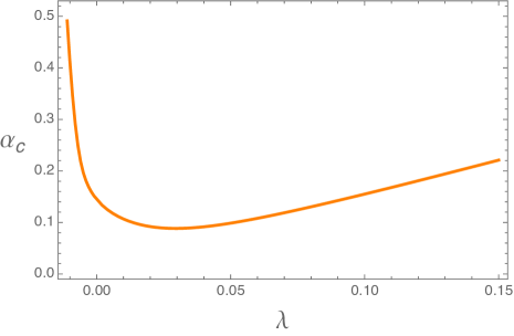
  Figure 2: The critical Chern-Simons coupling $\alpha_{c}$ as a function of $\lambda$ for the local minimum in the mass square being equal to the BF bound. Note that ${\alpha_{c}}_{\text{min}}=0.088$ at $\lambda=0.029.$ For fixed $\lambda$, when $\alpha_{c}<\alpha$, the minimal mass square is below the BF bound at value $k<k_{s}.$

• Now there might be three different momentum scales, $k_{s}$ defined in (3.18), $k_{*}$ in (3.31) and $k_{v}$ at which the BF bound is violated. These three scales may lead to an instability of the system for fixed $\alpha$ and $\lambda$. Since the reation (3.32) is always satisfied and the BF bound is always violated when $k>k_{s}$, we will not consider $k_{*}$ from now on.

  We can summarise as follows. The gravitational system around RN AdS black hole should have an instability as long as $\lambda\neq 0$. When $\alpha<\alpha_{c}$, the sources of instabilities are from $k_{s}$. When $\alpha_{c}<\alpha$, the sources of instabilities are from $k_{s}$ and also $k_{v}$.

  Let us illustrate the instabilities with the behaviour of $m_{1-}^{2}$ which is shown in Fig. 3. In both plots regions green and black refer to violation of BF bound, in the green region $m_{1-}^{2}<-3$, whereas in the black region $m_{1-}^{2}\in\mathcal{C}$ . When $\alpha$ takes values in the interval $0\leq\alpha<{\alpha_{c}}_{\text{min}}$ the instability is tuned by $k_{s}$, and for $\alpha>{\alpha_{c}}_{\text{min}}$ a new instability island (red region) appears in the middle of the stable (white) region. When $\alpha=0.21$, its behaviour is shown in the right plot. As similar to the the case $\alpha=0$ we always have instabilities from $k_{s}$ and $k_{*}$, while we also have a new instability island (red region) in which the mass square is below the BF bound. If we further increase $\alpha$, the unstable island become even bigger and will cross the $k=-k_{s}$ curve.

  

  

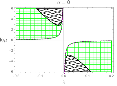
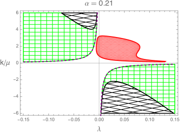
  Figure 3: The behaviour of $m_{1-}^{2}$ as a function of $k/\mu,\lambda$, at $\alpha=0$ (left) and $\alpha=0.21$ (right). In both plots, $m_{1-}^{2}$ is complex inside the black meshed region, below the BF bound in the green meshed region and above the BF bound in the rest of the white space. The dashed purple line corresponds with $k=-k_{s}$ in (3.18) and the green region are the instabilities inherited from the scale $k_{s}$. In the right plot $m_{1-}^{2}$ is also below the BF bound inside the red region (related to scale $k_{v}$) and this is related to gauge Chern-Simons term $\alpha$. The sector of $m_{1+}^{2}$ can be obtained by the transformation $k\to-k$. Since for real mass squares we have $m_{1\pm}^{2}\leq m_{2\pm}^{2}$, it is sufficient to study $m_{1}^{2}$ for the instability issue.

3.2 Instability and phase diagram

In the previous subsection, we studied the instability of the near horizon region of the extremal RN solution and we found the system has two different sources of instability. The first is intimate ligated with having $\alpha>\alpha_{c}$ and it will be the source of the typical bell curves that were found in the literature Nakamura:2009tf , the second exists if $\lambda\neq 0$ and essentially it is the BF bound violation when $k\to\pm k_{s}$. In this subsection, we will study the linear perturbation around the full Reissner-Nordström black hole in AdS₅ at both finite and zero temperature to study the effect of mixed gauge-gravitational anomaly on the stability of RN black hole. We will also comment on the nature of $k_{s}$.

Similar to the zero temperature near horizon analysis, we turn on the fluctuations (3.10) to study their equations in the full spacetime. We focus on the zero frequency limit to look for static solutions. It turns out we have $(a_{y}+ia_{z},h_{ty}+ih_{tz})$ sector decoupling from $(a_{y}-ia_{z},h_{ty}-ih_{tz})$ sector. Thus we consider the following static fluctuations around RN black hole geometry background (2.4) Donos:2012wi

$$\delta(ds^{2})=2Qdt\omega_{2}\,,~{}~{}~{}\delta A=a\omega_{2}$$ (3.37)

with the helical 1-forms of Bianchi VII₀ with pitch $k$

$$\omega_{1}=dx\,,~{}~{}~{}\omega_{2}=\cos(kx)dy+\sin(kx)dz\,,~{}~{}~{}\omega_{3}=\sin(kx)dy-\cos(kx)dz\,.$$ (3.38)

From the ansatz above, it is clear that the translational symmetry is preserved along $y$- and $z$- directions while broken along the $x$-direction. The residual symmetry is so-called helical symmetry, i.e. a one-parameter family with a translation in $x$- direction combined with rotation in ($y,z$) plane, $x\to x-\epsilon$, $(y,z)\to(y,z)+\epsilon k(z,-y)$.

After substituting (3.37) into the equations of motion (2.2, 2.3) we obtain

$$\Big{[}(r+4k\lambda\phi^{\prime})Q^{\prime}\Big{]}^{\prime}+\Big{(}-2r(k^{2}+4U)-8k\lambda(k^{2}-4U)\phi^{\prime}\Big{)}\frac{Q}{2r^{2}U}~{}~{}~{}~{}~{}$$ (3.39)

$$+\big{(}r\phi^{\prime}-\lambda(48k-\frac{24kU^{\prime}}{r}+2k\phi^{\prime 2})\big{)}a^{\prime}-4k\lambda U^{\prime\prime\prime}a = 0\,,$$

$$a^{\prime\prime}+\Big{(}\frac{U^{\prime}}{U}+\frac{1}{r}\Big{)}a^{\prime}-\big{(}k-8\alpha r\phi^{\prime}\big{)}\frac{k}{r^{2}U}a+\Big{(}r^{3}\phi^{\prime}-4k\lambda(r^{2}U^{\prime\prime}-2rU^{\prime}+2U)\Big{)}\frac{rQ^{\prime}-2Q}{r^{4}U} = 0\,.$$

First of all we observe that the system has the usual singularities at the boundary, horizon and a possible new singularity when $r_{s}+4k\lambda\phi^{\prime}=0$ has a real solution. In the case of having a real solution if $r_{s}$ is in between the horizon and the bulk, there will be subtleties to solve the system. Thus in the search of static normalisable solutions we will restrict the analysis to the cases when new singularity is behind the horizon $r_{s}<r_{+}$ or it does not exist. Later we will discuss the physical origin of this singularity and its possible implications in the full phase diagram of the theory.

Now let us analyse the near horizon and near boundary behaviours of the fields in (3.39). At finite temperature, near horizon $r\to r_{+}$, we have

$$Q=c_{1}(r-r_{+})+c_{2}(r-r_{+})^{2}+\dots\,,~{}~{}~{}~{}a=d_{0}+d_{1}(r-r_{+})\dots.$$ (3.40)

with

$$d_{1}=\frac{1}{r_{+}^{2}T}\left[\left(k^{2}-16\alpha k\mu\right)\frac{d_{0}}{4\pi}+\left(48k\lambda-\mu\right)\frac{c_{1}r_{+}}{2\pi}-36Tk\lambda c_{1}\right]$$ (3.41)

and

$$c_{2} = \frac{1}{4\pi Tr_{+}^{2}(r_{+}^{2}+8k\lambda\mu)}\left[\bigg{(}4\lambda k^{3}\mu+k^{2}\Big{(}\frac{r_{+}^{2}}{2}+1152\lambda^{2}(2r_{+}-3\pi T)^{2}\Big{)}+\right.$$ (3.42)

$$\left.~{}~{}~{}~{}~{}~{}~{}~{}48\lambda k\mu r_{+}(7\pi T-4r_{+})+2r_{+}^{2}\big{(}\mu^{2}-\pi r_{+}T\big{)}\bigg{)}c_{1}\right.+$$

$$\left.~{}~{}\Big{(}24\lambda k^{3}(2r_{+}-3\pi T)-k^{2}(\mu r_{+}+384\alpha\lambda\mu(2r_{+}-3\pi T))+\right.$$

$$\left.~{}~{}~{}~{}~{}~{}~{}~{}k\big{(}16\alpha\mu^{2}r_{+}+192\pi\lambda r_{+}T(8\pi T-7r_{+})\big{)}\Big{)}d_{0}\Big{]}\right.\,.$$

Notice that from Eq. (3.42) it is necessary to avoid the point $r_{+}^{2}+8k\lambda\mu=0$, which corresponds precisely with the finite temperature redefinition of the singular momentum $k=-k_{s}$, where

$$k_{s}(\lambda,T)=\frac{1}{288\mu\lambda}\left(3\pi T+\sqrt{6\mu^{2}+9\pi^{2}T^{2}}\right)^{2}.$$ (3.43)

This singular point appears as a consequence of the degeneration of the system at the characteristic surface $r_{s}+4k\lambda\phi^{\prime}=0$ in Eq. (3.39). In order to solve the system at this point, it would be necessary to find a new near horizon expansion. We leave the analysis of this case to the next subsection.

Near the boundary $r\to\infty$, we have

$$Q = Q_{0}r^{2}-\frac{k^{2}}{4}Q_{0}+\frac{k^{4}Q_{0}}{16}\frac{\ln r}{r^{2}}+\frac{Q_{2}}{r^{2}}+\ldots\,,$$

$$a = a_{0}-\frac{k^{2}a_{0}}{2}\frac{\ln r}{r^{2}}+\frac{a_{2}}{r^{2}}+\ldots\,.$$ (3.44)

We are interested in the normalisible solutions which signal the onset of instability, i.e. we look for solution with $a_{0}=Q_{0}=0.$ Thanks to the scaling properties of the background, we can always set $\mu=1$, the parameters $T$ and $k$ at which the static solution exists will be totally determined by the condition $a_{0}=Q_{0}=0.$ A convenient numerical method for seeking this static solution is the double shooting method. For details on the method, see e.g. Krikun:2013iha ; Kiritsis:2015hoa ; Andrade:2015iyf . The idea is as follows, one construct two independent solutions from the horizon to some matching point $r_{m}$ using the horizon data ($c_{1},d_{0}$). Then we shoot from the boundary to $r_{m}$ another pair of independent solutions using the boundary parameters $(a_{2},Q_{2})$ with $a_{0}=Q_{0}=0$. If the static solution exists, there will be a smooth connection between solutions at the matching point $r_{m}$, which is equivalent to the condition of vanishing the Wronskian at this point.

Starting from the normal state, i.e. RN black hole solution, we study the onset of $T/\mu$ at which static solution exists as a function of $k/\mu$ for different $(\alpha,\lambda)$. As shown in Fig. 4, we have the “bell-curve” phase diagrams of $T/\mu$ as a function of $k/\mu$ for finite $\alpha\simeq 0.213$ and different values of $\lambda$. The “bell-curve” behavior in the literature Nakamura:2009tf is not qualitatively modified by the mixed gauge-gravitational anomaly. Actually we find the bell-curves are consistent with the BF bound violation region at zero temperature, as shown in the red region of the right plot of Fig. 3. When we increase $\lambda$ from negative values the red island (see Fig. 3) becomes wider very fast, similar as we observe in left plot of Fig. 4. On the other hand, the upper momentum shows a turning point in Fig. 3 at some positive $\lambda$, such that the island becomes narrower. We observe a similar behavior in the right plot of Fig. 4. We also point out that the bell curves at $\lambda=-0.01,-0.012$ do not end at $T=0$, due to the fact that unstable region intersects $-k_{s}$ (Eq. 3.43), avoiding convergence of the numerics.

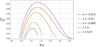
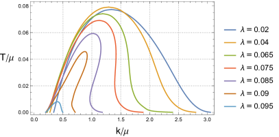
Figure 4: The “bell curve” phase diagram at $\alpha\simeq 0.213$ (i.e. $\alpha/\alpha_{c}(\lambda=0)=1.47$) for different values of $\lambda$. Note that when $\lambda=-0.01,-0.012$, the minimal temperature on the right side of bell-curve can not approach zero.

The static solution with the highest critical temperature $T_{c}$ which happens at $k_{c}$, corresponds to the onset of the spatially modulated phase. The behaviour of $T_{c}$ and $k_{c}$ depending on $\lambda$ can be found in Fig. 5. When $\lambda<0$, $T_{c}$ decreases, however the behaviour is not monotonic when $\lambda>0$. The corresponding $k_{c}/\mu$ behaves similarly as shown in the right plot. Hence, in the parameter space without possible singularity one can increase $\lambda$ or decrease $\lambda$ to tune $T_{c}$ to be zero. At the onset of this (possible) quantum phase transition, the pitch $k_{c}$ is nonzero.

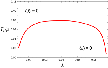
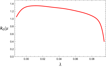
Figure 5: The critical temperature $T_{c}/\mu$ (left) which is the onset of the spatially modulated phase transition and the corresponding critical momentum $k_{c}/\mu$ (right) for different $\lambda$ when $\alpha\simeq 0.213$.

For the case without mixed gauge-gravitational anomaly it was proven in Nakamura:2009tf that the BF bound violation at zero temperature is a sufficient while not necessary condition for RN black hole to be unstable. To check the effect of the mixed anomaly we will construct static normalisable solutions at zero temperature. To do so, we build a near horizon expansion at zero temperature to be used in the numerical integration towards the boundary. The expansion reads

$$Q=q_{1}(r-r_{+})^{\beta_{1}}+q_{2}(r-r_{+})^{\beta_{2}}\,,~{}~{}~{}~{}~{}a=b_{1}(r-r_{+})^{\beta_{1}-1}+b_{2}(r-r_{+})^{\beta_{2}-1}$$ (3.45)

with

$$b_{j} = \frac{2\beta_{j}r_{+}(48k\lambda+\sqrt{6}r_{+})}{-12r_{+}^{2}\beta_{j}(\beta_{j}-1)+k^{2}+16\sqrt{6}kr_{+}\alpha}q_{j}\,,$$ (3.46)

$$\beta_{j} = \frac{1}{2}+\frac{\sqrt{3}}{6}\bigg{(}15+\frac{k^{2}}{r_{+}^{2}}+\frac{8\sqrt{6}k}{r_{+}}(\alpha-12\lambda)+\frac{384\sqrt{6}k\lambda}{r_{+}-8\sqrt{6}k\lambda}+$$

$$\frac{(-1)^{j}}{r_{+}^{2}}\sqrt{\bigg{(}-36r_{+}^{2}+8\sqrt{6}kr_{+}(\alpha-12\lambda)+\frac{48r_{+}^{3}}{r_{+}-8\sqrt{6}k\lambda}\bigg{)}^{2}+24k^{2}r_{+}\frac{(r_{+}+8\sqrt{6}k\lambda)^{2}}{r_{+}-8\sqrt{6}k\lambda}}~{}\Bigg{)}^{1/2}\,.$$

In units of $r_{+}=1$, i.e. $\mu=\sqrt{6}$, we have $\beta_{j}=\frac{1}{2}+\frac{\sqrt{3}}{6}\sqrt{3+m^{2}_{j-}}$ with $m^{2}_{j-}$ defined in (3.1). With this new near horizon condition and using the double shooting method, we find that static solutions with $k\leq k_{v}$ exist, which is shown in Fig. 6. In this plot we compare the momentum at which the BF bound is violated (red curve) with the lowest momentum found at which the static normalisable solution exists (blue curve). Note that when momentum takes value at the blue curve, it is above the BF bound (at least for $\lambda<0.06$). Thus we confirm for the system with the mixed gauge-gravitational anomaly, that BF violation at $T=0$ is a sufficient while not necessary condition for the instability.

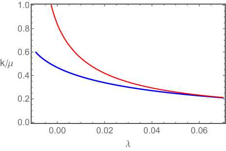
Figure 6: The blue line is the lowest critical value of momentum as a function of $\lambda$ (when $\alpha\simeq 0.213$) at which the static solution appears. It corresponds to the lower boundary of the bell curve in Fig. 4 at zero temperature. The red line is the boundary of $m^{2}_{1-}$ at which the BF bound is saturated.

3.2.1 Comments on the singularity and instability

Now let us comment on the other source of instability, $k_{s}$ at finite temperature. From (3.39) it is clear that $\lambda$ introduces a new “singular” point in the system at which the coefficient in front of $Q^{\prime\prime}$ vanishes. Besides the standard poles at the horizon ($r=r_{+}$) and the boundary ($r=\infty$), the new singular point appears as the solution of $r_{s}+4k\lambda\phi^{\prime}=0$, with the only real positive root being

$$r_{s}=\frac{1}{\sqrt{3}}(-2k\lambda\mu)^{1/4}\sqrt{3\pi T+\sqrt{9\pi^{2}T^{2}+6\mu^{2}}}\,,\quad\,k\lambda\mu<0\,.$$ (3.47)

There are two possibilities to avoid having a singularity in the bulk, either $k\lambda\mu>0$ ($r_{s}$ not real) or hiding the singular point behind the horizon ($r_{s}<r_{+}$), which imply

$$-\frac{1}{288}\left(3\pi T+\sqrt{6\mu^{2}+9\pi^{2}T^{2}}\right)^{2}<k\lambda\mu\,,$$ (3.48)

which at zero temperature reduces to $-\frac{1}{48}<\lambda k/\mu.$ Notice that the lower bound in (3.48) corresponds to $-k_{s}\lambda\mu$ with $k_{s}$ defined in Eq. (3.43). That gives the clear interpretation for $k_{s}$, as the momentum at which $r_{s}=r_{+}$.

Now let us make a generic discussion on the implication of the singularity. If we write an effective reduced action for fluctuations (3.37), we have

$$\mathcal{L}_{\text{eff}}\supset(r+4k\lambda\phi^{\prime})QQ^{\prime\prime}+\ldots.$$ (3.49)

When moving from the boundary to the horizon, Eq. (3.49) indicates that the kinetic term for $Q$ changes sign at $r=r_{s}$, suggesting therefore the existence of ghost-like modes.

Let us remind the reader that the full non-linear system is third order, that implies the holographic dictionary for the model should be properly studied and defined in detail. Also notice that the linearised problem around Reissner-Nordström is second order. If for example the charged black hole was a stationary axisymmetric-like, instead of a planar static one, the linear equations would be third order. On a background of this form, the singular point could disappear because the structure and existence of the characteristic surface is given by the coefficient of the highest derivative term in the equations. Of course, in this case a new problem emerge because the holographic dictionary needs to be understood.

From a top down point of view $\lambda$ should be small and treated as a perturbative parameter, which would solve the problem. For example, in $\mathcal{N}=4$ SYM, the chiral anomaly is of order $N_{c}^{2}$ while the mixed gauge-gravitational anomaly is zero, however, one might also attempt to add some flavors degrees of freedom to make the mixed gauge-gravitational anomaly $\lambda$ of order $N_{c}N_{f}$ Kimura:2011ef . Then we would have $\lambda/N_{c}^{2}\sim N_{f}/N_{c}\ll 1$. In the units $2\kappa^{2}=L=1$ that we use, this means the $\lambda$ term in (3.49) can be ignored. Nonetheless, our perspective is bottom up. Therefore, to better understand the physics of the singular surface we will study the case $r_{s}=r_{+}$ (i.e. $k=-k_{s}$), where no problematic sign in the kinetic term of the effective Lagrangian appears. The finite temperature near horizon expansion (3.40) has to be modified as follows

$$Q = (r-r_{+})^{\gamma_{1}}(q_{0}+...)+c_{0}+c_{1}(r-r_{+})+\dots\,,$$

$$a = (r-r_{+})^{\gamma_{1}}(a_{0}+...)+d_{0}+d_{1}(r-r_{+})+\dots\,,$$ (3.50)

with

$$\gamma_{1}=\frac{1}{2}\sqrt{\frac{3}{2}}\frac{\big{|}6r_{+}^{2}-5\mu^{2}\big{|}}{\sqrt{6\mu^{2}r_{+}^{2}-\mu^{4}}}\,,~{}~{}~{}~{}a_{0}=\frac{\text{sign}(6r_{+}^{2}-5\mu^{2})\sqrt{6}\,q_{0}}{\sqrt{6r_{+}^{2}-\mu^{2}}}\,,$$ (3.51)

where $(c_{i},d_{i})$ ($i=1,2,...$) are totally fixed by $(c_{0},d_{0})$. This expansion shows two problems, the first one is the presence of three integration constants ($q_{0},c_{0},d_{0}$), making the system undetermined. The second is even worst, each coefficients $(c_{i},d_{i})$ become singular when $T/\mu\simeq 0.05,0.08,0.14$, $0.36$, $0.53$, $0.72\ldots$ respectively.

In principle it is possible to understand our fluctuations around Reissner-Nordström as a special limit of the fully backreacted ansatz

$$ds^{2} = -ufdt^{2}+\frac{dr^{2}}{u}+h\omega_{1}^{2}+r^{2}e^{2\gamma}(\omega_{2}+Qdt)^{2}+r^{2}e^{-2\gamma}\omega_{3}^{2}$$ (3.52)

$$A = \phi dt+a\omega_{2}$$ (3.53)

with $\omega_{i}$ $(i=1,2,3)$ defined in (3.38). At the black hole horizon $u(r_{+})=Q(r_{+})=0$ have to be satisfied, which suggest the condition $c_{0}=0$ in the near horizon expansion (3.2.1), however we still have the problem of the singularities in the coefficients $(c_{i},d_{i})$. Anyhow after trying to find static solutions avoiding the singularities, we realized that no normalisable solution can be constructed.

Given the unreliability of the linear problem when $r_{s}=r_{+}$, we will proceed to compute the quasinormal modes for $r_{s}\lesssim r_{+}$. Considering the presence of the characteristic surface is insensitive to the values of $\alpha$, as we observe in Fig. 3, we will set it to zero. In Fig. 7 we show the lowest quasinormal modes after fixing the parameters as follow, $\mu=1$, $\lambda=1$ and $r_{+}=1$. The singular momentum in this case takes the value $k_{s}/(2\pi T)=-3/40$, the modes were computed for momenta within the values $k\in(k_{s}+4\times 10^{-4},-k_{s})(2\pi T)$. The second quasinormal mode (right plot) does not show any peculiarity in its trajectory in the complex frequency plane. On the other hand, the purely imaginary pole (left plot), which in the hydrodynamic regime obeys the dispersion relation $\omega\approx-i\frac{\eta}{\epsilon+P}k^{2}$, deviates from the parabolic behavior when the momentum approaches $k_{s}$. In fact, the closer we go to the singular momentum, the fastest the imaginary part grows, in consistency with the presence of an instability at $k=k_{s}$. Therefore, this naive quasinormal mode analysis suggests a relation of the singular point with a possible instability of the RN black hole.

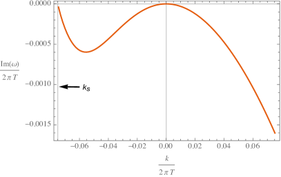
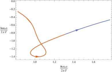
Figure 7: Left: Lowest purely imaginary quasinormal mode as a function of momentum. Right: Complex frequency plane for the second quasinormal mode parametrized by the momentum, blue and red lines correspond to positive and negative momentum respectively. The arrows indicate the direction the momentum grows or decreases. The singular momentum is $k_{s}/(2\pi T)=-0.075$. The parameters are fixed as $\mu=1$, $\lambda=1$, $\alpha=0$ and $r_{+}=1$.

On the other hand, we would also like to emphasize that the presence of the characteristic surface is a consequence of being at finite density, i.e. the Schwartzshild black hole does not have a singular momentum (see appendix A). That might be an indication that the RN black hole is not the real finite density groundstate of the system, and that the “good” background would propagate fluctuations without any characteristic surface in the bulk.

Finally, let us make an analogy to the holographic dual of a two dimensional pure gravitational anomaly, which is described by the three dimensional Einstein gravity with a gravitational Chern-Simons term, i.e. the so called topologically massive gravity (TMG) Kraus:2005zm . As it is well known anomaly-induced transport shows a lot of similarities between chiral four dimensional quantum field theories and the two dimensional one Jensen:2012kj . In particular, the mixed gauge-gravitational anomaly is the four dimensional cousin of the gravitational anomaly in two dimensions. The same is expected to be true for their holographic duals, i.e. the theory in consideration here (2.1) and TMG respectively. To make the analogies clearest let us enumerate them as follow

• Both TMG and the gravitational theory (2.1) are higher derivatives in the metric sector and the equations of motion are third order. On the TMG side, a lot of research have been done with finite Chern-Simons coupling and it is believed that for some values of the coupling it is a consistent holographic theory, without other higher derivative terms or other matter fields coming from string theory.

  In both cases the Chern-Simons couplings have been studied non-perturbatively. However, the consistency status is better understood in TMG, in Li:2008dq it was found that there always exist a bulk mode (either massless graviton or massive graviton) around AdS₃ with negative energy for generic Chern-Simons coupling except for the critical value, at which appropriate boundary conditions were established and a holographic duality in terms of a logarithmic CFT in Grumiller:2008qz was discussed. Subsequently it was conjectured that the stable backgrounds are given by the warped AdS₃ geometry Anninos:2008fx .

• Three and five dimensional Chern-Simons terms reproduce the right anomalous contribution in the Ward identities of a quantum field theory with either a pure gravitational anomaly in two dimensions or a mixed gauge-gravitational anomaly in four dimensions respectively.

• Due to the nature of the mixed gauge-gravitational Chern-Simons in 5-dimensions, either nontrivial gauge fields or finite temperature is needed in order to have a contribution into the equations of motion, in opposite with the TMG case, in which the Chern-Simons is purely gravitational. Therefore the analogous backgrounds to compare in the study should be AdS₅ black holes with AdS₃.

  The equations for the linearised graviton on AdS₅ are $\lambda$-independent, implying the stability and consistency of the linear problem as it happens with Einstein-Maxwell theory. At finite temperature but zero charge density, there is no signal of unstable modes in the five dimensional theory (see appendix A), and no singular point emerges in the bulk.

By the above analogy between TMG and the five dimensional gravitational theory (2.1) and the known studies on the consistency in TMG, one may expect that the five dimensional theory with finite Chern-Simons coupling, around Reissner-Nordström, is generically unstable but new stable groundstate could exist around which no puzzling singular momentum issue would emerge.

4 Conclusion and discussion

We have studied the perturbative instability for RN black hole in Einstein-Maxwell-Chern-Simons gravitational theory with a gravitational Chern-Simons term at both zero temperature and finite temperature. We have established that there exist two sources of instabilities. One is the BF bound violation on the AdS₂ near horizon geometry at zero temperature (similar to pure CS gauge theory case), and the resulting phase diagram at finite temperature is a bell curve which only exist when $\alpha>{\alpha_{c}}_{\text{min}}$. Another instability is associated to $k_{s}$ and close to it there are always unstable modes. Moreover, this instability happens at arbitrary gravitational Chern-Simons coupling $\lambda$. At finite temperature we studied the origin of this singular momentum and found that it indicates whether a characteristic surface appears in the bulk or behind the horizon, in particular, when $k=k_{s}$ the singular point coincides with the horizon. The presence of such surface in the bulk turns unreliable the IR boundary value problem, maybe related to the presence of ghost-like modes and/or potentially causality issues.

Thus our study suggests that the linearized problem of the theory with the gravitational Chern-Simons term around Reissner-Nordström is unreliable, for non-perturbative Chern-Simons coupling. However, considering the theory around AdS₅ is well defined, and the Schwartzshild black hole seems not to suffer of instabilities, at least at the quasinormal modes level. It could be possible that for finite charge density a new well defined background may exist, as it is conjecture to happen in TMG with the case of AdS₃ and warp AdS₃.

This project ended with several open questions that we hopefully will address in the future to properly understand the system. An incomplete list reads

• Stability, causality and consistency analysis of the full theory, taking into account the possible presence of the Orstrogodski instability Woodard:2015zca , positivity of time delay Camanho:2014apa and the method of characteristics Reall:2014pwa .

• Check the existence of a reliable new ground state at finite density for finite values of $\lambda$, and check its stability.

• Study the fully backreacted solution of the spatially modulated phase for the parameters inside the bell curve in Fig. 4.

• Consider a consistent truncation of SUGRA including a gravitational Chern-Simons term Cremonini:2008tw ; Myers:2009ij ; Aharony:1999rz and analyse the spatially modulated instability in this theory.

• A 4D gravitational analogue of the spatially modulated instability in 5D has been studied in the context of AdS/CFT in e.g. Donos:2011bh ; Bergman:2011rf . By including the effect of gravitational Chern-Simons term (e.g. Saremi:2011ab ; Liu:2014gto ), one may attempt to expect that a similar instability will happen.

Acknowledgments

We thank R. G. Cai, L. Y. Hung, K. Landsteiner, A. Marini, J. Ren, Y. W. Sun for helpful discussions. Y.L. has been supported by the Thousand Young Talents Program of China and grants ZG216S17A5 and KG12003301 from Beihang University. Y.L. thanks IFT-UAM/CSIC for the warm hospitality during the completion of the present work.

Appendix A QNMs for Schwartzshild black hole background

In this appendix, we shall show that the gravitational theory (2.1) with gravitational Chern-Simons term seems to be stable around the Schwartzschild black hole background, by the computation of the quasinormal modes spectra at zero density and finite or zero temperature.

By studying the $\lambda$ effects on the spectrum of quasi-normal modes (QNMs) around the Schwartzschild black hole background, which encodes the locations of poles of the retarded two-point correlators of the energy-momentum and axial current operators, we will show the poles are in the lower half of the complex frequency plane.

We consider the case of zero axial charge density. On the gravity side, we have the Schwartzschild AdS black hole

$$ds^{2}=-r^{2}f(r)dt^{2}+\frac{dr^{2}}{r^{2}f(r)}+r^{2}(dx^{2}+dy^{2}+dz^{2})\,,~{}~{}~{}A=0\,,$$ (A.54)

with $f(r)=1-\frac{r_{0}^{4}}{r^{4}}$. We introduce the metric and gauge field fluctuations of form $\delta g_{\mu\nu}=h_{\mu\nu}e^{-i\omega t+ikz},\delta A_{\mu}=a_{\mu}e^{-i\omega t+ikz}.$ We work in the radial gauge $h_{r\mu}=a_{r}=0$ and classify the fluctuations according to their transformation properties in the $(x,y)-$plane as follows,

• Helicity 2: $h_{xy},\frac{1}{2}(h_{xx}-h_{yy})$ ;

• Helicity 1: $h_{t\alpha},h_{z\alpha},a_{\alpha}$ with $\alpha\in(x,y)$ ;

• Helicity 0: $h_{tt},h_{tz},h_{xx}+h_{yy},h_{zz},a_{t},a_{z}$ .

For both, helicity 2 and helicity 0 sectors, there is no effect from $\lambda$ on the linearised EOM and they satisfied the same equations as the Einstein-Maxwell gravity case. There is no instability from these sectors Kovtun:2005ev . However, the gravitational anomaly term does have effects on the helicity 1 fluctuations. The independent equations are

$$h^{\prime\prime}_{t\alpha}+\frac{1}{r}h^{\prime}_{t\alpha}-\frac{k^{2}+4r^{2}f}{r^{4}f}h_{t\alpha}-\frac{k\omega}{r^{4}f}h_{z\alpha}+12ik\lambda f^{\prime}\epsilon^{\alpha\beta}\Big{(}a^{\prime}_{\beta}-\frac{2}{r}a_{\beta}\Big{)} = 0\,,$$ (A.55)

$$\frac{\omega}{f}h^{\prime}_{t\alpha}-\frac{2\omega}{rf}h_{t\alpha}+kh^{\prime}_{z\alpha}-\frac{2k}{r}h_{z\alpha}+\frac{12ik\lambda\omega f^{\prime}}{f}\epsilon^{\alpha\beta}a_{\beta} = 0\,,$$ (A.56)

$$a^{\prime\prime}_{\beta}+\Big{(}\frac{3}{r}+\frac{f^{\prime}}{f}\Big{)}a^{\prime}_{\beta}+\frac{1}{r^{4}f}\Big{(}\frac{\omega^{2}}{f}-k^{2}\Big{)}a_{\beta}+12ik\lambda\frac{f^{\prime}}{r^{2}f}\epsilon^{\beta\alpha}\Big{(}h^{\prime}_{t\alpha}-\frac{2}{r}h_{t\alpha}\Big{)} = 0\,.$$ (A.57)

where $\alpha\in(x,y)$ and $\epsilon^{xy}=-\epsilon^{yx}=1$.

The gauge invariant quantities for the fluctuations are constructed as

$$Z_{\alpha}=k\frac{h_{t\alpha}}{r^{2}}+\omega\frac{h_{z\alpha}}{r^{2}}\,,~{}~{}~{}E_{\alpha}=\omega a_{\alpha}\,.$$ (A.58)

In terms of the gauge invariant fields the above fluctuation equations can be written as

$$Z_{x}^{\prime\prime}+C_{1}Z_{x}^{\prime}+C_{2}Z_{x}+C_{3}E_{y}^{\prime}+C_{4}E_{y} = 0\,,$$

$$E_{y}^{\prime\prime}+D_{1}E_{y}^{\prime}+D_{2}E_{y}+D_{3}Z_{x}^{\prime} = 0\,,$$

$$Z_{y}^{\prime\prime}+C_{1}Z_{y}^{\prime}+C_{2}Z_{y}-C_{3}E_{x}^{\prime}-C_{4}E_{x} = 0\,,$$

$$E_{x}^{\prime\prime}+D_{1}E_{x}^{\prime}+D_{2}E_{x}-D_{3}Z_{y}^{\prime} = 0\,,$$ (A.59)

where the coefficients read

$$C_{1} = \frac{5}{r}-\frac{\omega^{2}}{k^{2}f-\omega^{2}}\frac{f^{\prime}}{f}\,,~{}~{}~{}~{}C_{2}=-\frac{1}{r^{4}f^{2}}\Big{(}k^{2}f-\omega^{2}\Big{)}\,,~{}~{}~{}~{}C_{3}=12i\lambda\frac{k^{2}f^{\prime}}{\omega r^{2}}\,,$$

$$C_{4} = -12i\lambda\frac{k^{2}f^{\prime}}{\omega r^{2}}\Big{(}\frac{2}{r}+\frac{\omega^{2}}{k^{2}f-\omega^{2}}\frac{f^{\prime}}{f}\Big{)}\,,~{}~{}~{}~{}D_{1}=\frac{3}{r}+\frac{f^{\prime}}{f}\,,$$

$$D_{2} = \frac{1}{r^{4}f^{2}}(\omega^{2}-k^{2}f)+144\lambda^{2}\frac{k^{2}\omega^{2}}{k^{2}f-\omega^{2}}\frac{f^{\prime 2}}{r^{2}f}\,,~{}~{}~{}~{}D_{3}=-12i\lambda\frac{k^{2}\omega f^{\prime}}{k^{2}f-\omega^{2}}\,.$$ (A.60)

Redefining the fields in term of $Z_{\pm}=Z_{x}\pm iZ_{y},E_{\pm}=E_{x}\pm iE_{y}$, we have two set of decoupled equations given the helicity of the fields

$$Z_{\pm}^{\prime\prime}+C_{1}Z_{\pm}^{\prime}+C_{2}Z_{\pm}\pm(-iC_{3})E_{\pm}^{\prime}\pm(-iC_{4})E_{\pm} = 0\,,$$ (A.61)

$$E_{\pm}^{\prime\prime}+D_{1}E_{\pm}^{\prime}+D_{2}E_{\pm}\pm(iD_{3})Z_{\pm}^{\prime} = 0\,.$$ (A.62)

In order to solve for the QNM spectra for the above coupled differential equations, we expand the fields near the horizon

$$Z_{\pm}=\Big{(}1-\frac{r_{0}^{4}}{r^{4}}\Big{)}^{-\frac{i\omega}{4r_{0}}}(z_{in}+...)\,,~{}~{}~{}~{}E_{\pm}=\Big{(}1-\frac{r_{0}^{4}}{r^{4}}\Big{)}^{-\frac{i\omega}{4r_{0}}}(e_{in}+...)\,,$$ (A.63)

and select the infalling modes. Near the AdS₅ boundary we have

$$Z_{\pm}=z_{0}(1+\dots)+\frac{z_{1}}{r^{4}}(1+\dots)\,,~{}~{}~{}~{}E_{\pm}=e_{0}(1+\dots)+\frac{e_{1}}{r^{2}}(1+\dots)\,.$$ (A.64)

The quasinormal frequencies are the values of complex $\omega$ for fixed real $k$, $z_{0}=e_{0}=0$. When $\omega/r_{0},k/r_{0}\ll 1$, following Kovtun:2005ev we can define $\zeta=\frac{\omega}{k}$, and solve the above equations peturbatively on $\zeta,k$. After doing so, we obtain the perturbative solutions in $\zeta,k$, which have a near boundary expansion

$$E_{\pm} \simeq \big{(}1-\frac{4ir_{0}\zeta}{k}\big{)}\beta+\mathcal{O}(k^{2})+\mathcal{O}\big{(}\frac{1}{r^{4}}\big{)},$$ (A.65)

$$Z_{\pm} \simeq \big{(}1-\frac{4ir_{0}\zeta}{k}\big{)}\alpha+\mathcal{O}(k^{2})+\mathcal{O}\big{(}\frac{1}{r^{2}}\big{)}.$$ (A.66)

The normalizability condition then implies $\omega=-i\frac{k^{2}}{4r_{0}}$, which does not depend on $\lambda$.

Next, we fixed $\frac{k}{4\pi T}=1$ and compute the three lowest quasinormal frequencies as a function of $\lambda$, we show them in figure 8. The Re$\frac{\omega}{2r_{0}}$ is shown in the right plot and the Im$\frac{\omega}{2r_{0}}$ at the left. In the left plot we observe that the quasinormal modes are always located in the lower half plane. We also notice that quasinormal modes are symmetric under $\lambda\to-\lambda$. Thus we can claim that the linear problem around Schwartzschild is well defined, and no instabilities seem to appear at the quasinormal frequencies level.

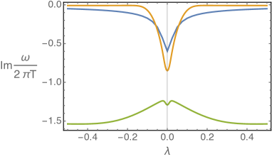
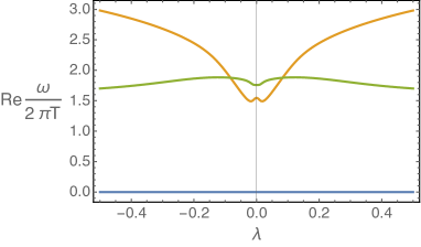
Figure 8: The imaginary and real parts of quasinormal frequency as a function of $\lambda$ at fixed $k=4\pi T$. The blue line is for the Diffusion pole, the orange line is for the first QNMs and the green line is the second QNMs.

References

- (1) S. Nakamura, H. Ooguri and C. S. Park, Gravity Dual of Spatially Modulated Phase, Phys. Rev. D 81, 044018 (2010), [arXiv:0911.0679].
- (2) H. Ooguri and C. S. Park, Holographic End-Point of Spatially Modulated Phase Transition, Phys. Rev. D 82, 126001 (2010), [arXiv:1007.3737].
- (3) A. Donos and J. P. Gauntlett, Black holes dual to helical current phases, Phys. Rev. D 86, 064010 (2012), [arXiv:1204.1734].
-
(4)
J. Zaanen, Y. W. Sun, Y. Liu and K. Schalm,
Holographic Duality in Condensed Matter Physics,
Cambridge University Press, 2015.
M. Ammon and J. Erdmenger, Gauge/Gravity Duality: Foundations and Applications, Cambridge University Press, 2015.
J.Casalderrey-Solana, H. Liu, D. Mateos, K. Rajagopal and U. A. Wiedemann, Gauge/String Duality, Hot QCD and Heavy Ion Collisions, Cambridge University Press, 2014. - (5) L. Alvarez-Gaume and E. Witten, Gravitational Anomalies, Nucl. Phys. B 234, 269 (1984).
-
(6)
D. T. Son and P. Surowka,
Hydrodynamics with Triangle Anomalies,
Phys. Rev. Lett. 103, 191601 (2009),
[arXiv:0906.5044].
Y. Neiman and Y. Oz, Relativistic Hydrodynamics with General Anomalous Charges, JHEP 1103, 023 (2011), [arXiv:1011.5107]. - (7) K. Jensen, R. Loganayagam and A. Yarom, Thermodynamics, gravitational anomalies and cones, JHEP 1302, 088 (2013), [arXiv:1207.5824].
- (8) K. Landsteiner, E. Megias and F. Pena-Benitez, Gravitational Anomaly and Transport, Phys. Rev. Lett. 107, 021601 (2011), [arXiv:1103.5006].
- (9) K. Landsteiner, Y. Liu and Y. W. Sun, Odd viscosity in the quantum critical region of a holographic Weyl semimetal, Phys. Rev. Lett. 117, no. 8, 081604 (2016), [arXiv:1604.01346].
- (10) A. Lucas, R. A. Davison and S. Sachdev, Hydrodynamic theory of thermoelectric transport and negative magnetoresistance in Weyl semimetals, Proc. Nat. Acad. Sci. 113, 9463 (2016), [arXiv:1604.08598].
- (11) K. Landsteiner, E. Megias, L. Melgar and F. Pena-Benitez, Holographic Gravitational Anomaly and Chiral Vortical Effect, JHEP 1109, 121 (2011), [arXiv:1107.0368].
- (12) M. Brigante, H. Liu, R. C. Myers, S. Shenker and S. Yaida, The Viscosity Bound and Causality Violation, Phys. Rev. Lett. 100, 191601 (2008), [arXiv:0802.3318].
- (13) R. C. Myers, S. Sachdev and A. Singh, Holographic Quantum Critical Transport without Self-Duality, Phys. Rev. D 83, 066017 (2011), [arXiv:1010.0443].
- (14) X. O. Camanho, J. D. Edelstein, J. Maldacena and A. Zhiboedov, Causality Constraints on Corrections to the Graviton Three-Point Coupling, JHEP 1602, 020 (2016), [arXiv:1407.5597].
-
(15)
S. Chapman, Y. Neiman and Y. Oz,
Fluid/Gravity Correspondence, Local Wald Entropy Current and Gravitational Anomaly,
JHEP 1207, 128 (2012),
[arXiv:1202.2469].
E. Megias and F. Pena-Benitez, Holographic Gravitational Anomaly in First and Second Order Hydrodynamics, JHEP 1305, 115 (2013), [arXiv:1304.5529].
K. Landsteiner, E. Megias and F. Pena-Benitez, Frequency dependence of the Chiral Vortical Effect, Phys. Rev. D 90, no. 6, 065026 (2014), [arXiv:1312.1204].
T. Azeyanagi, R. Loganayagam, G. S. Ng and M. J. Rodriguez, Covariant Noether Charge for Higher Dimensional Chern-Simons Terms, JHEP 1505, 041 (2015), [arXiv:1407.6364].
K. Rajagopal and A. V. Sadofyev, Chiral drag force, JHEP 1510, 018 (2015), [arXiv:1505.07379].
T. Azeyanagi, R. Loganayagam and G. S. Ng, Holographic Entanglement for Chern-Simons Terms, JHEP 1702, 001 (2017) [arXiv:1507.02298]. - (16) A. Bhattacharyya, L. Cheng and L. Y. Hung, Relative Entropy, Mixed Gauge-Gravitational Anomaly and Causality, JHEP 1607, 121 (2016), [arXiv:1605.02553].
- (17) S. Cremonini, K. Hanaki, J. T. Liu and P. Szepietowski, Black holes in five-dimensional gauged supergravity with higher derivatives, JHEP 0912, 045 (2009), [arXiv:0812.3572].
- (18) S. Takeuchi, Modulated Instability in Five-Dimensional U(1) Charged AdS Black Hole with R2-term, JHEP 1201, 160 (2012), [arXiv:1108.2064].
- (19) H. Reall, N. Tanahashi and B. Way, Causality and Hyperbolicity of Lovelock Theories, Class. Quant. Grav. 31, 205005 (2014), [arXiv:1406.3379].
- (20) A. Krikun, Charge density wave instability in holographic d-wave superconductor, JHEP 1404, 135 (2014), [arXiv:1312.1588].
- (21) E. Kiritsis and L. Li, Holographic Competition of Phases and Superconductivity, JHEP 1601, 147 (2016), [arXiv:1510.00020].
- (22) T. Andrade and A. Krikun, Commensurability effects in holographic homogeneous lattices, [arXiv:1512.02465].
- (23) M. Lippert, R. Meyer and A. Taliotis, A holographic model for the fractional quantum Hall effect, JHEP 1501, 023 (2015), [arXiv:1409.1369].
- (24) T. Kimura and T. Nishioka, The Chiral Heat Effect, Prog. Theor. Phys. 127, 1009 (2012), [arXiv:1109.6331].
- (25) P. Kraus and F. Larsen, Holographic gravitational anomalies, JHEP 0601, 022 (2006), [hep-th/0508218].
- (26) W. Li, W. Song and A. Strominger, Chiral Gravity in Three Dimensions, JHEP 0804, 082 (2008), [arXiv:0801.4566].
-
(27)
D. Grumiller and N. Johansson,
Instability in cosmological topologically massive gravity at the chiral point,
JHEP 0807, 134 (2008),
[arXiv:0805.2610].
A. Maloney, W. Song and A. Strominger, Chiral Gravity, Log Gravity and Extremal CFT, Phys. Rev. D 81, 064007 (2010), [arXiv:0903.4573].
K. Skenderis, M. Taylor and B. C. van Rees, Topologically Massive Gravity and the AdS/CFT Correspondence, JHEP 0909, 045 (2009), [arXiv:0906.4926]. - (28) D. Anninos, W. Li, M. Padi, W. Song and A. Strominger, Warped AdS(3) Black Holes, JHEP 0903, 130 (2009), [arXiv:0807.3040].
- (29) R. P. Woodard, Ostrogradsky’s theorem on Hamiltonian instability, Scholarpedia 10, no. 8, 32243 (2015), [arXiv:1506.02210].
- (30) R. C. Myers, M. F. Paulos and A. Sinha, Holographic Hydrodynamics with a Chemical Potential, JHEP 0906, 006 (2009), [arXiv:0903.2834].
- (31) O. Aharony, J. Pawelczyk, S. Theisen and S. Yankielowicz, A Note on anomalies in the AdS / CFT correspondence, Phys. Rev. D 60, 066001 (1999), [hep-th/9901134].
- (32) A. Donos and J. P. Gauntlett, Holographic striped phases, JHEP 1108, 140 (2011), [arXiv:1106.2004].
- (33) O. Bergman, N. Jokela, G. Lifschytz and M. Lippert, Striped instability of a holographic Fermi-like liquid, JHEP 1110, 034 (2011), [arXiv:1106.3883].
- (34) O. Saremi and D. T. Son, Hall viscosity from gauge/gravity duality, JHEP 1204, 091 (2012), [arXiv:1103.4851].
- (35) H. Liu, H. Ooguri and B. Stoica, Hall Viscosity and Angular Momentum in Gapless Holographic Models, Phys. Rev. D 90, no. 8, 086007 (2014), [arXiv:1403.6047].
- (36) P. K. Kovtun and A. O. Starinets, Quasinormal modes and holography, Phys. Rev. D 72, 086009 (2005), [hep-th/0506184].