Almost all quantum channels are equidistant

Abstract

In this work we analyze properties of generic quantum channels in the case of large system size. We use random matrix theory and free probability to show that the distance between two independent random channels converges to a constant value as the dimension of the system grows larger. As a measure of the distance we use the diamond norm. In the case of a flat Hilbert-Schmidt distribution on quantum channels, we obtain that the distance converges to $\frac{1}{2}+\frac{2}{\pi}$, giving also an estimate for the maximum success probability for distinguishing the channels. We also consider the problem of distinguishing two random unitary rotations.

1 Introduction

For any linear map $\Phi:M_{d_{1}}(\mathbb{C})\to M_{d_{2}}(\mathbb{C})$, we define its Choi-Jamiołkowski matrix as

$$J(\Phi):=\sum_{i,j=1}^{d_{1}}|i\rangle\langle j|\otimes\Phi(|i\rangle\langle j|)\in M_{d_{1}}(\mathbb{C})\otimes M_{d_{2}}(\mathbb{C}).$$ (1)

This isomorphism was first studied by Choi [11] and Jamiołkowski [26]. Note that some authors prefer to add a normalization factor of $d_{1}^{-1}$ if front of the expression for $J(\Phi)$. Other authors use the other order for the tensor product factors, a choice resulting in an awkward order for the space in which $J(\Phi)$ lives.

The rank of the matrix $J(\Phi)$ is called the Choi rank of $\Phi$; it is the minimum number $r$ such that the map $\Phi$ can be written as

$$\Phi(\cdot)=\sum_{i=1}^{r}A_{i}\cdot B_{i}^{*},$$

for some operators $A_{i},B_{i}\in M_{d_{2}\times d_{1}}(\mathbb{C})$.

The diamond norm was introduced in Quantum Information Theory by Kitaev [25, Section 3.3] as a counterpart to the $1$-norm in the task of distinguishing quantum channels. First, define the $1\to 1$ norm of a linear map $\Phi:M_{d_{!}}(\mathbb{C})\to M_{d_{2}}(\mathbb{C})$ as

$$\|\Phi\|_{1\to 1}:=\sum_{X\neq 0}\frac{\|\Phi(X)\|_{1}}{\|X\|_{1}}.$$

Kitaev noticed that the $1\to 1$ norm is not stable under tensor products (as it can easily be seen by looking at the transposition map), and considered the following ’’regularization‘‘:

$$\|\Phi\|_{\diamond}:=\sup_{n\geq 1}\|\Phi\otimes\operatorname{id}_{n}\|_{1\to 1}.$$

In operator theory, the diamond norm was known before as the completely bounded trace norm; indeed, the $1\to 1$ norm of an operator is the $\infty\to\infty$ norm of its dual, hence the diamond norm of $\Phi$ is equal to the completely bounded (operator) norm of $\Phi^{*}$ (see [35, Chapter 3]).

We shall need two simple properties of the diamond norm. First, note that the supremum in the definition can be replaced by taking the value $n=d_{1}$ (recall that $d_{1}$ is the dimension of the input Hilbert space of the linear map $\Phi$); actually, one could also take $n$ equal to the Choi rank of the map $\Phi$, see [44, Theorem 3.3] or [45, Theorem 3.66]. Second, using the fact that the extremal points of the unit ball of the $1$-norm are unit rank matrices, we always have

$$\|\Phi\|_{\diamond}=\sup\{\|(\Phi\otimes\operatorname{id}_{d_{1}})(|x\rangle\langle y|)\|_{1}\,:\,x,y\in\mathbb{C}^{d_{1}}\otimes\mathbb{C}^{d_{1}},\,\|x\|=\|y\|=1\}.$$

Moreover, if the map $\Phi$ is Hermiticity-preserving (e.g. $\Phi$ is the difference of two quantum channels), one can optimize over $x=y$ in the formula above, see [45, Theorem 3.53].

Given a map $\Phi$, it is in general difficult to compute its diamond norm. Computationally, there is a semidefinite program for the diamond norm, [46], which has a simple form and which has been implemented in various places (see, e.g. [29]). We will bound the diamond norm in terms of the partial trace of the absolute value of the Choi-Jamiołkowski matrix.

The diamond norm finds applications in the problem of quantum channel discrimination. Suppose we have an experiment in which our goal is to distinguish between two quantum channels $\Phi$ and $\Psi$. Each of the channels may appear with probability $\frac{1}{2}$. Then, celebrated results by Helstrom [21], Holevo [23], and Kitaev [25] give an upper bound on the probability of correct discrimination

$$p\leq\frac{1}{2}+\frac{1}{4}\|\Phi-\Psi\|_{\diamond}.$$ (2)

The main goal of this work is study the asymptotic behavior of the diamond norm of the difference of two independent quantum channels. To achieve this, in Section 2 we find a new upper bound of on the diamond norm of a general map. In our case, it has a nice form

$$\|\Phi-\Psi\|_{\diamond}\leq\|\mathrm{Tr}_{2}|J(\Phi-\Psi)|\|_{\infty}.$$ (3)

Next, in Section 4.1 we prove that the well known lower bound on the diamond norm, $\|J(\Phi-\Psi)\|_{1}\leq\|\Phi-\Psi\|_{\diamond}$, converges to a finite value for random independent quantum channels $\Phi$ and $\Psi$ in the limit $d_{1,2}\to\infty$. We obtain that for channel sampled from the flat Hilbert-Schmidt distribution, the value of the lower bound is

$$\lim_{d_{1,2}\to\infty}\frac{1}{d_{1}}\|J(\Phi-\Psi)\|_{1}=\frac{1}{2}+\frac{2}{\pi}\;\;\mathrm{a.s.}$$ (4)

Finally, in Section 4.2 we show that the upper bound (3) also converges to the same value as the lower bound. From these results, we infer that for independent random quantum channels sampled from the Hilbert-Schmidt distribution, we have

$$\lim_{d_{1,2}\to\infty}\|\Phi-\Psi\|_{\diamond}=\frac{1}{2}+\frac{2}{\pi}\;\;\mathrm{a.s.}$$ (5)

In particular, the optimal success probability of distinguishing the two channels (in the asymptotical regime) is

$$p\leq\frac{1}{2}+\frac{1}{4}\left(\frac{1}{2}+\frac{2}{\pi}\right)=\frac{5}{8}+\frac{1}{2\pi}\approx 0.7842.$$ (6)

Several generalizations of this type of results are gathered in Theorem 7, the main result of this paper.

In Sections 5 and 7 we address respectively two similar problems: distinguishing a random quantum channels from the maximally depolarizing channel and distinguishing two random unitary channels.

2 Some useful bounds for the diamond norm

We discuss in this section some bounds for the diamond norm. For a matrix $X$, we denote by $\sqrt{X^{*}X}$ and $\sqrt{XX^{*}}$ its right and left absolute values, i.e.

$$\sqrt{X^{*}X}=V\Sigma V^{*}\qquad\text{ and }\qquad\sqrt{XX^{*}}=U\Sigma U^{*},$$

when $X=U\Sigma V^{*}$ is the SVD of $X$. In the case where $X$ is self-adjoint, we obviously have $\sqrt{X^{*}X}=\sqrt{XX^{*}}$.

In the result below, the lower bound is well-known, while the upper bound appeared in a weaker and less general form in [27, Theorem 2].

Proposition 1

For any linear map $\Phi:M_{d_{1}}(\mathbb{C})\to M_{d_{2}}(\mathbb{C})$, we have

1. $$\frac{1}{d_{1}}\|J(\Phi)\|_{1}\leq\|\Phi\|_{\diamond}\leq\frac{\|\operatorname{Tr}_{2}\sqrt{J(\Phi)^{*}J(\Phi)}\|_{\infty}+\|\operatorname{Tr}_{2}\sqrt{J(\Phi)J(\Phi)^{*}}\|_{\infty}}{2}.$$ (7)

2. Above bounds are equal iff the PSD matrices $\varphi:=\operatorname{Tr}_{2}\sqrt{J(\Phi)^{*}J(\Phi)}$ and $\psi:=\operatorname{Tr}_{2}\sqrt{J(\Phi)J(\Phi)^{*}}$ are both scalar.

Proof. We start by proving item 1. Consider the semidefinite programs for the diamond norm given in [46, Section 3.2]:

Primal problem

maximize: $$\frac{1}{2}\langle X,J(\Phi)\rangle+\frac{1}{2}\langle X^{*},J(\Phi)^{*}\rangle$$

subject to: $$\begin{bmatrix}\rho_{0}\otimes I_{d_{2}}&X\\ X^{*}&\rho_{1}\otimes I_{d_{2}}\end{bmatrix}\geq 0$$

$$\rho_{0},\rho_{1}\in M_{d_{1}}^{1,+}(\mathbb{C})$$

$$X\in M_{d_{1}d_{2}}(\mathbb{C})$$

Dual problem

minimize: $$\frac{1}{2}\|\operatorname{Tr}_{2}Y_{0}\|_{\infty}+\frac{1}{2}\|\operatorname{Tr}_{2}Y_{1}\|_{\infty}$$

subject to: $$\begin{bmatrix}Y_{0}&-J(\Phi)\\ -J(\Phi)^{*}&Y_{1}\end{bmatrix}\geq 0$$

$$Y_{0},Y_{1}\in M_{d_{1}d_{2}}^{+}(\mathbb{C})$$

The lower and upper bounds will follow from very simple feasible points for the primal, resp. the dual problems. Let $J(\Phi)=U\Sigma V^{*}$ be a SVD of the Choi-Jamiołkowski state of the linear map. For the primal problem, consider the feasible point $\rho_{0,1}=d_{1}^{-1}I_{d_{1}}$ and $X=d_{1}^{-1}UV^{*}$. The value of the primal problem at this point is

$$\frac{1}{2d_{1}}\langle UV^{*},UV^{*}|J(\Phi)|\rangle+\frac{1}{2d_{1}}\langle VU^{*},|J(\Phi)|VU^{*}\rangle=\frac{1}{d_{1}}\|J(\Phi)\|_{1},$$

showing the lower bound.

For the upper bound, set $Y_{0}=\sqrt{J(\Phi)J(\Phi)^{*}}=U\Sigma U^{*}$ and $Y_{1}=\sqrt{J(\Phi)^{*}J(\Phi)}=V\Sigma V^{*}$, both PSD matrices. The condition in the dual problem is satisfied:

$$\begin{bmatrix}Y_{0}&-J(\Phi)\\ -J(\Phi)^{*}&Y_{1}\end{bmatrix}=\begin{bmatrix}U\Sigma U^{*}&-U\Sigma V^{*}\\ -V\Sigma U^{*}&V\Sigma V^{*}\end{bmatrix}=\begin{bmatrix}U&0\\ 0&V\end{bmatrix}\cdot\left(\begin{bmatrix}1&-1\\ -1&1\end{bmatrix}\otimes\Sigma\right)\cdot\begin{bmatrix}U&0\\ 0&V\end{bmatrix}^{*}\geq 0,$$

and the proof of item 1 is complete.

To show statement in item 2 note that the lower bound in (7) can be rewritten as

$$\frac{1}{d_{1}}\|J(\Phi)\|_{1}=\frac{1}{d_{1}}\operatorname{Tr}\varphi=\frac{1}{d_{1}}\operatorname{Tr}\psi,$$

and the two bounds are equal exactly when the spectra of $\varphi$ and $\psi$ are flat. This is also the necessary and sufficient condition for the saturation of the lower bound, see [30, 32].    

Corollary 2

If the map $\Phi$ is Hermiticity-preserving (i.e. the matrix $J(\Phi)$ is self-adjoint), the inequality in the statement reads simply

$$\frac{1}{d_{1}}\|J(\Phi)\|_{1}\leq\|\Phi\|_{\diamond}\leq\|\operatorname{Tr}_{2}|J(\Phi)|\|_{\infty}.$$

Let us now characterize the maps $\Phi$ for which the upper bound in (7) is saturated. Since our proof is SDP-based, we use the same technique as in [30, Theorem 18].

Proposition 3

A map $\Phi$ saturates the upper bound in (7) iff there exist unit vectors $a,b\in\mathbb{C}^{d_{1}}$ and a unitary operator $W\in\mathcal{U}_{d_{1}d_{2}}$ with the following properties (we write $J=J(\Phi)$):

• The vector $a$ achieves the operator norm for $\operatorname{Tr}_{2}\sqrt{JJ^{*}}$

• The vector $b$ achieves the operator norm for $\operatorname{Tr}_{2}\sqrt{J^{*}J}$

• $(aa^{*}\otimes I_{d_{2}})W=W(bb^{*}\otimes I_{d_{2}})$

• $J=WP$ for some positive semidefinite operator $P$; in other words, $W$ is the angular part in some polar decomposition of $J$.

Proof. The reasoning follows closely the proof of [30, Theorem 18], we only sketch the main lines. Writing the SDP in the standard form (see also [46, Section 3.2] for the notation). Optimal matrices for the primal and the dual program are, respectively

$$A_{opt}=\begin{bmatrix}\rho_{0}&.&.&.\\ .&\rho_{1}&.&.\\ .&.&\rho_{0}\otimes I_{d_{2}}&W\\ .&.&W^{*}&\rho_{1}\otimes I_{d_{2}}\end{bmatrix},B_{opt}=\frac{1}{2}\begin{bmatrix}\|\operatorname{Tr}_{2}\sqrt{JJ^{*}}\|_{\infty}&.&.&.\\ .&\|\operatorname{Tr}_{2}\sqrt{J^{*}J}\|_{\infty}&.&.\\ .&.&\sqrt{JJ^{*}}&.\\ .&.&.&\sqrt{J^{*}J}\end{bmatrix},$$

where . denotes an unimportant element. Since strong duality holds for our primal-dual pair [46, Section 3.2], complementary slackness holds and we have

$$\left(\|\operatorname{Tr}_{2}\sqrt{JJ^{*}}\|_{\infty}I-\operatorname{Tr}_{2}\sqrt{JJ^{*}}\right)\rho_{0} =0$$

$$\left(\|\operatorname{Tr}_{2}\sqrt{J^{*}J}\|_{\infty}I-\operatorname{Tr}_{2}\sqrt{J^{*}J}\right)\rho_{1} =0$$

$$U\Sigma U^{*}R =U\Sigma V^{*}(\rho_{1}\otimes I_{d_{2}})$$

$$V\Sigma V^{*}R^{*} =V\Sigma U^{*}(\rho_{0}\otimes I_{d_{2}}),$$

where $J=U\Sigma V^{*}$ is the singular value decomposition of $J$. Using an approximation argument, we can assume $J$ (and thus $\Sigma$) is invertible, and thus $W=UV^{*}$ is unique. We then set $\rho_{0}=aa^{*}$ and $\rho_{1}=bb^{*}$, and the result follows.    

Remark 4

The upper bound in (7) can be seen as a strengthening of the following inequality $\|\Phi\|_{\diamond}\leq\|J(\Phi)\|_{1}$, which already appeared in the literature (e.g. [45, Section 3.4]). Indeed, again in terms of $\varphi$ and $\psi$, we have $\|\varphi\|_{\infty}\leq\|\varphi\|_{1}$ and $\|\psi\|_{\infty}\leq\|\psi\|_{1}$. The inequality in (7) is much stronger: for example, it is always saturated for tensor product matrices $J=J_{1}\otimes J_{2}$ ($W$ from the result above is also product), whereas the weaker inequality $\|\Phi\|_{\diamond}\leq\|J(\Phi)\|_{1}$ is saturated in this case only when $J_{1}$ has rank one, see [30, 32].

3 Discriminating random quantum channels

3.1 Probability distributions on the set of quantum channels

There are several ways to endow the convex body of quantum channels with probability distributions. In this section, we discuss several possibilities and the relations between them.

Recall that the Choi-Jamiołkowski isomorphism puts into correspondence a quantum channel $\Phi:M_{d_{1}}(\mathbb{C})\to M_{d_{2}}(\mathbb{C})$ with a bipartite matrix $J(\Phi)\in M_{d_{1}}(\mathbb{C})\otimes M_{d_{2}}(\mathbb{C})$ having the following two properties

• $J(\Phi)$ is positive semidefinite

• $\operatorname{Tr}_{2}J(\Phi)=I_{d_{1}}$.

The above two properties correspond, respectively, to the fact that $\Phi$ is complete positive and trace preserving. Hence, it is natural to consider probability measures on quantum channels obtained as the image measures of probabilities on the set of bipartite matrices with the above properties. Henceforth we will denote the set of all quantum channels as $\Theta(d_{1},d_{2})$.

Given some fixed dimensions $d_{1},d_{2}$ and a parameter $s\geq d_{1}d_{2}$, let $G\in M_{d_{1}d_{2}\times s}(\mathbb{C})$ be a random matrix having i.i.d. standard complex Gaussian entries; such a matrix is called a Ginibre random matrix. Define then

$$W :=GG^{*}\in M_{d_{1}}(\mathbb{C})\otimes M_{d_{2}}(\mathbb{C})$$ (8)

$$D :=\left((\mathrm{Tr}_{2}W)^{-1/2}\otimes I_{d_{2}}\right)W\left((\mathrm{Tr}_{2}W)^{-1/2}\otimes I_{d_{2}}\right)\in M_{d_{1}}(\mathbb{C})\otimes M_{d_{2}}(\mathbb{C}).$$ (9)

The random matrices $W$ and $D$ are called, respectively, Wishart and partially normalized Wishart. The inverse square root in the definition of $D$ uses the Moore-Penrose convention if $W$ is not invertible; note however that this is almost never the case, since the Wishart matrices with parameter $s$ larger than its size is invertible with unit probability. It is for this reason we do not consider here smaller integer parameters $s$. Note that the matrix $D$ satisfies the two conditions discussed above: it is positive semidefinite and its partial trace over the second tensor factor is the identity:

$$\operatorname{Tr}_{2}D =\operatorname{Tr}_{2}\left[\left((\mathrm{Tr}_{2}W)^{-1/2}\otimes I_{d_{2}}\right)W\left((\mathrm{Tr}_{2}W)^{-1/2}\otimes I_{d_{2}}\right)\right]$$

$$=(\mathrm{Tr}_{2}W)^{-1/2}\left(\operatorname{Tr}_{2}W\right)(\mathrm{Tr}_{2}W)^{-1/2}=I_{d_{1}}.$$

Hence, there exists a quantum channel $\Phi_{G}$, such that $J(\Phi_{G})=D$ (note that $D$, and thus $\Phi$ are functions of the original Ginibre random matrix $G$).

Definition 1

The image measure of the Gaussian standard measure through the map $G\mapsto\Phi_{G}$ defined in (8), (9) and the equation $J(\Phi_{G})=D$ is called the partially normalized Wishart measure and is denoted by $\gamma^{W}_{d_{1},d_{2},s}$.

Of particular interest is the case $s=d_{1}d_{2}$; the measure obtained in this case will be called the Hilbert-Schmidt measure as it is induced from the Hilbert-Schmidt measure on the space of bipartite quantum states by partial normalization [10] and will be denoted by $\gamma^{HS}$ (see [41] for the case of random quantum states).

Let us mention here also other measures in the space of quantum operations discussed in the literature. One can use the Stinespring dilation theorem [42]: for any channel $\Phi:M_{d_{1}}(\mathbb{C})\to M_{d_{2}}(\mathbb{C})$, there exists, for some given $s\leq d_{1}d_{2}$, an isometry $V:\mathbb{C}^{d_{1}}\to\mathbb{C}^{d_{2}}\otimes\mathbb{C}^{s}$ such that

$$\Phi(\cdot)=\operatorname{Tr}_{2}(V\cdot V^{*}).$$ (10)

Definition 2

For any integer parameter $s$, let $\gamma^{Haar}_{d_{1},d_{2},s}$ be the image measure of the Haar distribution on isometries $V$ through the map in (10).

Finally, one can consider the Lebesgue measure on the convex body of quantum channels, $\gamma^{L}_{d_{1},d_{2}}$ which leads to the Euclidean geometry of this set [43]. In this work, we shall however be concerned only with the measure $\gamma^{W}$ coming from normalized Wishart matrices. The relations between all these probability measures on the set of quantum channels shall be investigated in some future work.

3.2 The (two–parameter) subtracted Marc̆enko–Pastur distribution

In this section we introduce and study the basic properties of a two-parameter family of probability measures which will appear later in the paper. This family generalizes the symmetrized Marc̆enko–Pastur distributions from [38], see also [34, 18] for other occurrences of some special cases. Before we start, recall that the Marc̆enko–Pastur (of free Poisson) distribution of parameter $x>0$ has density given by [33, Proposition 12.11]

$$d\mathcal{MP}_{x}=\max(1-x,0)\delta_{0}+\frac{\sqrt{4x-(u-1-x)^{2}}}{2\pi u}1_{[a,b]}(u)\,du,$$

where $a=(\sqrt{x}-1)^{2}$ and $b=(\sqrt{x}+1)^{2}$.

Definition 3

Let $a,b$ be two free random variables having Marc̆enko–Pastur distributions with respective parameters $x$ and $y$. The distribution of the random variable $a/x-b/y$ is called the subtracted Marc̆enko–Pastur distribution with parameters $x,y$ and is denoted by $\mathcal{SMP}_{x,y}$. In other words,

$$\mathcal{SMP}_{x,y}=D_{1/x}\mathcal{MP}_{x}\boxplus D_{-1/y}\mathcal{MP}_{y},$$ (11)

where $D_{c}\mathcal{P}$ is a distribution of a random variable $Z^{\prime}=cZ$ provided $Z$ is distributed according to $\mathcal{P}$.

We have the following result.

Proposition 5

Let $W_{x}$ (resp. $W_{y}$) be two Wishart matrices of parameters $(d,s_{x})$ (resp $(d,s_{y})$). Assuming that $s_{x}/d\to x$ and $s_{y}/d\to y$ for some constants $x,y>0$, then, almost surely as $d\to\infty$, we have

$$\lim_{d\to\infty}\|(xd^{2})^{-1}W_{x}-(yd^{2})^{-1}W_{y}\|_{1}=\int|u|\,d\mathcal{SMP}_{x,y}(u)=:\Delta(x,y).$$

Proof. The proof follows from standard arguments in random matrix theory, and from the fact that the Schatten $1$-norm is the sum of the singular values, which are the absolute values of the eigenvalues in the case of self-adjoint matrices.    

We gather next some properties of the probability measure $\mathcal{SMP}_{x,y}$. Examples of this distribution are shown in Fig. 1.

Proposition 6

Let $x,y>0$. Then,

1. If $x+y<1$, then the probability measure $\mathcal{SMP}_{x,y}$ has exactly one atom, located at 0, of mass $1-(x+y)$. If $x+y\geq 1$, then $\mathcal{SMP}_{x,y}$ is absolutely continuous with respect to the Lebesgue measure on $\mathbb{R}$.

2. Define

   $$\begin{split}a_{x,y}&=(x-y)(2x+y)(x+2y)\\ b_{x,y}&=2x^{3}+2y^{3}+(x+y)^{2}+xy(x+y+2)\\ c_{x,y}&=(x-y)(x+y+1-2(x+y)^{2})\\ U_{x,y}(u)&=-u^{3}a_{x,y}+3u^{2}b_{x,y}+3uc_{x,y}+2(x+y-1)^{3}\\ T_{x,y}(u)&=(x+y-1-u(x-y))^{2}+3u(y-x+uxy)\\ Y_{x,y}(u)&=U_{x,y}(u)+\sqrt{\left[U_{x,y}(u)\right]^{2}-4\left[T_{x,y}(u)\right]^{3}}.\end{split}$$ (12)

   The support of the absolutely continuous part of $\mathcal{SMP}_{x,y}$ is the set

   $$\{u\,:\,\left[U_{x,y}(u)\right]^{2}-4\left[T_{x,y}(u)\right]^{3}\geq 0\}.$$ (13)

3. On its support, the density of $\mathcal{SMP}_{x,y}$ is given by

   $$\frac{d\mathcal{SMP}_{x,y}}{du}=\left|\frac{\left[Y_{x,y}(u)\right]^{\frac{2}{3}}-2^{\frac{2}{3}}T_{x,y}(u)}{2^{\frac{4}{3}}\sqrt{3}\pi u\left[Y_{x,y}(u)\right]^{\frac{1}{3}}}\right|.$$ (14)

Proof. The statement regarding the atoms follows from [5, Theorem 7.4]. The formula for the density and equation (13) comes from Stieltjes inversion, see e.g. [33, Lecture 12]. Indeed, since the $R$-transform of the Marc̆enko–Pastur distribution $\mathcal{MP}_{x}$ reads $R_{x}(z)=x/(1-z)$, the $R$-transform of the subtracted measure reads

$$R(z)=\frac{1}{1-z/x}-\frac{1}{1+z/y}.$$

The Cauchy transform $G$ of $\mathcal{SMP}_{x,y}$ can be obtained from the functional equation

$$R(G)+1/G=z.$$

This leads to the following third degree polynomial equation for $G$

$$zG^{3}+[x(1-z)+y(1+z)-1]G^{2}+(x-y-xyz)G+xy=0.$$

Using Cardano‘s formulas for the solutions of a cubic, we can solve this equation and obtain a solution $G(z)$. The last step is to perform the Stieltjes inversion

$$\mathcal{SMP}_{x,y}(u)=-\frac{1}{\pi}\lim_{\varepsilon\to 0}\Im G(u+\mathrm{i}\varepsilon).$$

 

In the case where $x=y$, some of the formulas from the result above become simpler (see also [38]). When $x=y>1/2$, the distribution of $\mathcal{SMP}_{x,x}$ is supported between

$$u_{\pm}=\pm\frac{\sqrt{2+10x-x^{2}+(x+4)^{\frac{3}{2}}\sqrt{x}}}{\sqrt{2}x}.$$

When $x=y\leq 1/2$, $\mathcal{SMP}_{x,x}$ has an atom in $0$ of mass $1-2x$, and its absolutely continuous part is supported on $[u_{-},v_{-}]\cup[v_{+},u_{+}]$, where

$$v_{\pm}=\pm\frac{\sqrt{2+10x-x^{2}-(x+4)^{\frac{3}{2}}\sqrt{x}}}{\sqrt{2}x}.$$

Finally, in the case when $x=y=1$, which corresponds to a flat Hilbert-Schmidt measure on the set of quantum channels, we get that $\Delta(1,1)=\frac{1}{2}+\frac{2}{\pi}$.

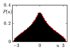
(a) $x=1$, $y=1$

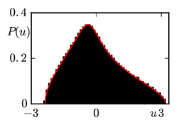
(b) $x=1$, $y=2$

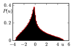
(c) $x=0.5$, $y=1$

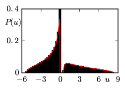
(d) $x=0.25$, $y=0.5$

Figure 1: Subtracted Marc̆enko–Pastur distribution for (x, y)=(1,1) (a), (1, 2) (b), (0.5, 1) (c) and (0.25, 0.5) (d). The red curve is the plot of (14), while the black histogram corresponds to Monte Carlo simulations. Notice the Dirac mass at zero in the last example.

4 The asymptotic diamond norm of the difference of two independent random quantum channels

We state here the main result of the paper. For the proof, see the following two subsections, each providing one of the bounds needed to conclude.

Theorem 7

Let $\Phi$, resp. $\Psi$, be two independent random quantum channels from $\Theta(d_{1},d_{2})$ having $\gamma^{W}$distribution with parameters $(d_{1},d_{2},s_{x})$, resp. $(d_{1},d_{2},s_{y})$. Then, almost surely as $d_{1,2}\to\infty$ in such a way that $s_{x}/(d_{1}d_{2})\to x$, $s_{y}/(d_{1}d_{2})\to y$ (for some positive constants $x,y$), and $d_{1}\ll d_{2}^{2}$,

$$\lim_{d_{1,2}\to\infty}\|\Phi-\Psi\|_{\diamond}=\Delta(x,y)=\int|u|\,d\mathcal{SMP}_{x,y}(u).$$

Proof. The proof follows from Theorems 10 and 14, which give the same asymptotic value.    

Remark 8

We think that the condition $d_{1}\ll d_{2}^{2}$ in the statement is purely technical, and could be replaced by a much weaker condition.

Corollary 9

Combining Theorem 7 with Hellstrom‘s theorem for quantum channels, we get that the optimal probability $p$ of distinguishing two quantum channels is equal to:

$$p=\frac{5}{8}+\frac{1}{2\pi}.$$ (15)

Additionally, any maximally entangled state may be used to achieve this value.

4.1 The lower bound

In this section we compute the asymptotic value of the lower bound in Theorem 7. Given two random quantum channels $\Phi,\Psi$, we are interested in the asymptotic value of the quantity $d_{1}^{-1}\|J(\Phi-\Psi)\|_{1}$.

Theorem 10

Let $\Phi$, resp. $\Psi$, be two independent random quantum channels from $\Theta(d_{1},d_{2})$ having $\gamma^{W}$distribution with parameters $(d_{1},d_{2},s_{x})$, resp. $(d_{1},d_{2},s_{y})$. Then, almost surely as $d_{1,2}\to\infty$ in such a way that $s_{x}/(d_{1}d_{2})\to x$ and $s_{y}/(d_{1}d_{2})\to y$ for some positive constants $x,y$,

$$\lim_{d_{1,2}\to\infty}\frac{1}{d_{1}}\|J(\Phi-\Psi)\|_{1}=\Delta(x,y)=\int|u|\,d\mathcal{SMP}_{x,y}(u).$$

The proof of this result (as well as the proof of Theorem 10) uses in a crucial manner the approximation result for partially normalized Wishart matrices.

Proposition 11

Let $W\in M_{d_{1}}(\mathbb{C})\otimes M_{d_{2}}(\mathbb{C})$ a random Wishart matrix of parameters $(d_{1}d_{2},s)$, and consider its ’’partial normalization‘‘ $D$ as in (9). Then, almost surely as $d_{1,2}\to\infty$ in such a way that $s\sim td_{1}d_{2}$ for a fixed parameter $t>0$,

$$\big{\|}D-(td_{1}d_{2}^{2})^{-1}W\big{\|}_{\infty}=O(d_{2}^{-2}).$$

Note that in the statement above, the matrix $W$ is not normalized; we have

$$\frac{1}{d_{1}d_{2}}\sum_{i=1}^{d_{1}d_{2}}\delta_{\lambda_{i}((d_{1}d_{2})^{-1}W)}\to\mathcal{MP}_{t},$$

the Marc̆henko–Pastur distribution of parameter $t$. In other words, $W=GG^{*}$, where $G$ is random matrix of size $d_{1}d_{2}\times s$, having i.i.d. standard complex Gaussian entries.

Let us introduce the random matrices

$$X=(td_{1}d_{2}^{2})^{-1}\operatorname{Tr}_{2}W\quad\text{and}\quad Y=X^{-1/2}\otimes I_{d_{2}}.$$

The first observation we make is that the random matrix $X$ is also a (rescaled) Wishart matrix. Indeed, the partial trace operation can be seen, via duality, as a matrix product, so we can write

$$X=\frac{1}{td_{1}d_{2}^{2}}\tilde{G}\tilde{G}^{*},$$

where $\tilde{G}$ is a complex Gaussian matrix of size $d_{1}\times d_{1}s$; remember that $s$ scales like $td_{1}d_{2}$. Since, in our model, both $d_{1}$, $d_{2}$ grow to infinity, the behavior of the random matrix $X$ follows from [15].

Lemma 12

As $d_{1,2}\to\infty$, the random matrix $\sqrt{t}d_{2}(X-I_{d_{1}})$ converges in moments toward a standard semicircular distribution. Moreover, almost surely, the limiting eigenvalues converge to the edges of the support of the limiting distribution:

$$\sqrt{t}d_{2}\lambda_{\min}(X-I_{d_{1}}) \rightarrow-2$$

$$\sqrt{t}d_{2}\lambda_{\max}(X-I_{d_{1}}) \rightarrow 2.$$

Proof. The proof is a direct application of [15, Corollary 2.5 and Theorem 2.7]; we just need to check the normalization factors. In the setting of [15, Section 2], the Wishart matrices are not normalized, so the convergence result deals with the random matrices (here $d=d_{1}$ and $s=td_{1}d_{2}^{2}$)

$$\sqrt{t}d_{1}d_{2}\left(\frac{\tilde{G}\tilde{G}^{*}}{td_{1}^{2}d_{2}^{2}}-\frac{I_{d_{1}}}{d_{1}}\right)=\sqrt{t}d_{2}(X-I_{d_{1}}).$$

 

We look now for a similar result for the matrix $Y$; the result follows by functional calculus.

Lemma 13

Almost surely as $d_{1,2}\to\infty$, the limiting eigenvalues of the random matrix $\sqrt{t}d_{2}(Y-I_{d_{1}d_{2}})$ converge respectively to $\pm 1$:

$$\sqrt{t}d_{2}\lambda_{\min}(Y-I_{d_{1}d_{2}}) \rightarrow-1$$

$$\sqrt{t}d_{2}\lambda_{\max}(Y-I_{d_{1}d_{2}}) \rightarrow 1.$$

Proof. By functional calculus, we have $\lambda_{\max}(Y)=[\lambda_{\min}(X)]^{-1/2}$, so, using the previous lemma, we get

$$\lambda_{\max}(Y)=\left[1-\frac{2}{\sqrt{t}d_{2}}+o(d_{2}^{-1})\right]^{-1/2}=1+\frac{1}{2}\frac{2}{\sqrt{t}d_{2}}+o(d_{2}^{-1}),$$

and the conclusion follows. The case of $\lambda_{\min}(Y)$ is similar.    

We have now all the ingredients to prove Proposition 11.

Proof of Proposition 11. We have

$$\big{\|}D-(td_{1}d_{2}^{2})^{-1}W\big{\|}_{\infty} =\big{\|}(td_{1}d_{2}^{2})^{-1}\left(YWY-W\right)\big{\|}_{\infty}$$

$$=(td_{1}d_{2}^{2})^{-1}\big{\|}(Y_{i}-I)W_{i}Y_{i}+W_{i}(Y_{i}-I)\big{\|}_{\infty}$$

$$\leq(td_{1}d_{2}^{2})^{-1}\|Y_{i}-I\|_{\infty}\|W_{i}\|_{\infty}\left(1+\|Y_{i}\|_{\infty}\right)$$

$$=\frac{t^{-3/2}}{d_{2}^{2}}\cdot\sqrt{t}d_{2}\|Y_{i}-I\|_{\infty}\cdot(d_{1}d_{2})^{-1}\|W_{i}\|_{\infty}\cdot\left(1+\|Y_{i}\|_{\infty}\right).$$

Note that, almost surely, the three random matrix norms in the last equation above converge respectively to the following finite quantities

$$\sqrt{t}d_{2}\|Y_{i}-I\|_{\infty} \to 1$$

$$(d_{1}d_{2})^{-1}\|W_{i}\|_{\infty} \to(\sqrt{t}+1)^{2}$$

$$1+\|Y_{i}\|_{\infty} \to 1.$$

The first and the third limit above follow from Lemma 13, while the second one is the Bai-Yin theorem [3, Theorem 2] or [2, Theorem 5.11].    

Let us now prove Theorem 10.

Proof of Theorem 10. The result follows easily by approximating the partially normalized Wishart matrices with scalar normalizations. By the triangle inequality, with $D_{x}:=J(\Phi)$ and $D_{y}:=J(\Psi)$, we have

$$\left|\frac{1}{d_{1}}\|D_{x}-D_{y}\|_{1}-\frac{1}{d_{1}}\|(xd_{1}d_{2}^{2})^{-1}W_{x}-(yd_{1}d_{2}^{2})^{-1}W_{y}\|_{1}\right|$$

$$\qquad\qquad\leq\frac{1}{d_{1}}\|D_{x}-(xd_{1}d_{2}^{2})^{-1}W_{x}\|_{1}+\frac{1}{d_{1}}\|D_{y}-(yd_{1}d_{2}^{2})^{-1}W_{y}\|_{1}$$

$$\qquad\qquad\leq d_{2}\|D_{x}-(xd_{1}d_{2}^{2})^{-1}W_{x}\|_{\infty}+d_{2}\|D_{y}-(yd_{1}d_{2}^{2})^{-1}W_{y}\|_{\infty}.$$

The conclusion follows from Propositions 5 and 11.    

4.2 The upper bound

The core technical result of this work consists of deriving the asymptotic value of the upper bound in Theorem 7. Given two random quantum channels $\Phi,\Psi$, we are interested in the asymptotic value of the quantity $\|\operatorname{Tr}_{2}|J(\Phi-\Psi)|\|_{\infty}$.

Theorem 14

Let $\Phi$, resp. $\Psi$, be two independent random quantum channels from $\Theta(d_{1},d_{2})$ having $\gamma^{W}$distribution with parameters $(d_{1},d_{2},s_{x})$, resp. $(d_{1},d_{2},s_{y})$. Then, almost surely as $d_{1,2}\to\infty$ in such a way that $s_{x}/(d_{1}d_{2})\to x$, $s_{y}/(d_{1}d_{2})\to y$ (for some positive constants $x,y$), and $d_{1}/d_{2}^{2}\to 0$,

$$\lim_{d_{1,2}\to\infty}\|\operatorname{Tr}_{2}|J(\Phi-\Psi)|\|_{\infty}=\Delta(x,y)=\int|u|\,d\mathcal{SMP}_{x,y}(u).$$

The proof of Theorem 14 is presented at the end of this Section. It is based on the following lemma which appears in [17]; see also [7, Eq. (5.10)] or [6, Chapter X].

Lemma 15

For any matrices $A,B$ of size $d$, the following holds:

$$\|\ |A|-|B|\ \|_{\infty}\leq C\log d\ \|A-B\|_{\infty},$$ (16)

for a universal constant $C$ which does not depend on the dimension $d$.

For the sake of completeness, we give here a proof, relying on a similar estimate for the Schatten classes proved in [17].

Proof. Using [17, Theorem 8], we have, for any $p\in[2,\infty)$:

$$\|\ |A|-|B|\ \|_{\infty} \leq\|\ |A|-|B|\ \|_{p}$$

$$\leq 4(1+cp)\|A-B\|_{p}$$

$$\leq 4(1+cp)d^{1/p}\|A-B\|_{\infty},$$

for some universal constant $c\geq 1$. Choosing $p=\log d$ gives the desired bound, for $d$ large enough. The case of small values of $d$ is obtained by a standard embedding argument.    

Proof of Theorem 14. Using the triangle inequality and Lemma 15, we first prove an approximation result (as before, we write $D_{x}:=J(\Phi)$ and $D_{y}:=J(\Psi)$):

$$\big{|}\ \|\ \mathrm{Tr}_{2}|D_{x} -D_{y}|\ \|_{\infty}-\|\ \mathrm{Tr}_{2}|(xd_{1}d_{2}^{2})^{-1}W_{x}-(yd_{1}d_{2}^{2})^{-1}W_{y}|\ \|_{\infty}\ \big{|}$$

$$\qquad\leq\big{\|}\mathrm{Tr}_{2}|D_{x}-D_{y}|-\mathrm{Tr}_{2}|(xd_{1}d_{2}^{2})^{-1}W_{x}-(yd_{1}d_{2}^{2})^{-1}W_{y}|\big{\|}_{\infty}$$

$$\qquad=\big{\|}\mathrm{Tr}_{2}\left(|D_{x}-D_{y}|-|(xd_{1}d_{2}^{2})^{-1}W_{x}-(yd_{1}d_{2}^{2})^{-1}W_{y}|\right)\big{\|}_{\infty}$$

$$\qquad\leq d_{2}\big{\|}\ |D_{x}-D_{y}|-|(xd_{1}d_{2}^{2})^{-1}W_{x}-(yd_{1}d_{2}^{2})^{-1}W_{y}|\ \big{\|}_{\infty}$$

$$\qquad\leq Cd_{2}\log(d_{1}d_{2})\big{\|}(D_{x}-D_{y})-((xd_{1}d_{2}^{2})^{-1}W_{x}-(yd_{1}d_{2}^{2})^{-1}W_{y})\big{\|}_{\infty}$$

$$\qquad\leq Cd_{2}\log(d_{1}d_{2})\left(\big{\|}D_{x}-(xd_{1}d_{2}^{2})^{-1}W_{x}\big{\|}_{\infty}+\big{\|}D_{y}-(yd_{1}d_{2}^{2})^{-1}W_{y}\big{\|}_{\infty}\right)$$

$$\qquad=\frac{\log(d_{1}d_{2})}{d_{2}}O(1)\to 0,$$

where we have used Proposition 11 and the fact that $d_{1}\ll d_{2}^{2}\implies\log(d_{1})\ll d_{2}$. This proves the approximation result, and we focus now on the simpler case of Wishart matrices. Let us define

$$Z :=(xd_{1}d_{2})^{-1}W_{x}-(yd_{1}d_{2})^{-1}W_{y}$$

$$\tilde{Z}_{1} :=\operatorname{tr}_{2}(|Z|)=\operatorname{Tr}_{2}|(xd_{1}d_{2}^{2})^{-1}W_{x}-(yd_{1}d_{2}^{2})^{-1}W_{y}|$$

It follows from [22, Proposition 4.4.9] that the random matrix $Z$ converges almost surely (see Appendix A for the definition of almost sure convergence for a sequence of random matrices) to a non-commutative random variable having distribution $\mathcal{SMP}_{x,y}$, see (11). Moreover, using a standard strong convergence argument [31], the extremal eigenvalues of $Z$ converge almost surely to the extremal points of the support of the limiting probability measure $\mathcal{SMP}_{x,y}$. Hence, the almost sure convergence extends from the traces of the powers of $Z$ to any continuous bounded function (on the support of $\mathcal{SMP}_{x,y}$), in particular to the absolute value, i.e. to $|Z|$. From Proposition 23, the asymptotic spectrum of the random matrix $\tilde{Z}_{1}$ is flat, with all the eigenvalues being equal to

$$a=\lim_{d_{1},d_{2}\to\infty}\mathbb{E}\frac{\operatorname{Tr}|(xd_{1}d_{2})^{-1}W_{x}-(yd_{1}d_{2})^{-1}W_{y}|}{d_{1}d_{2}}=\int|u|d\mathcal{SMP}_{x,y}(u),$$

which, by Proposition 5, is equal to $\Delta(x,y)$, finishing the proof.

 

5 Distance to the depolarizing channel

In this section we derive the asymptotic distance between a random quantum channel $\Phi$ and the maximally depolarizing channel

$$\Psi_{\text{dep}}:M_{d_{1}}(\mathbb{C})\to M_{d_{2}}(\mathbb{C}),\qquad\Psi_{\text{dep}}(X)=\frac{\operatorname{Tr}(X)}{d_{2}}I_{d_{2}}.$$

Let us define the function $g:(1/4,\infty)\to(0,\infty)$

$$g(x) :=\frac{3}{2}-x+\frac{\sqrt{4x-1}(2x+1)}{2\pi x}$$

$$\qquad-\frac{1}{\pi}\left((x-1)\operatorname{arctan}\left(\frac{3x-1}{(x-1)\sqrt{4x-1}}\right)+\operatorname{arctan}\left(\sqrt{4x-1}\right)+x\operatorname{arctan}\left(\frac{1}{\sqrt{4x-1}}\right)\right).$$

Theorem 16

Let $\Phi$ a random quantum channel from $\Theta(d_{1},d_{2})$ having distribution $\gamma^{W}$ with parameters $(d_{1},d_{2},s_{x})$. Then, almost surely as $d_{1},d_{2}\to\infty$ and $s_{x}\sim xd_{1}d_{2}$, we have

$$\lim_{d_{1},d_{2}\to\infty}\|\Phi-\Psi_{\text{dep}}\|_{\diamond}=\int\left|\frac{u}{x}-1\right|d\mathcal{MP}_{x}(u)=\begin{cases}2(1-x)&\qquad\text{ if }x\in(0,1/4]\\ g(x)&\qquad\text{ if }x\in(1/4,1)\\ g(x)+x-1&\qquad\text{ if }x\in[1,\infty).\end{cases}$$ (17)

In the case $x=1$, the limit above reads $3\sqrt{3}/(2\pi)$.

Remark 17

We plot in Figure 2 the value of the limit in (17) as a function of $x$. One can show that the limit is a decreasing function of $x$, converging to $0$ as $x\to\infty$. The function behaves as $8/(3\pi)x^{-1/2}$ as $x\to\infty$.

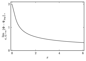
Figure 2: The asymptotic diamond-norm distance between a random quantum channel and the maximally depolarizing channel as a function of the channel parameter $x$.

Proof. We analyze separately the lower bound and the upper bound from Proposition 1. First, let us denote by $D_{x}$ the Choi-Jamiołkowski matrix of the channel $\Phi$, and note that $J(\Psi_{\text{dep}})=d_{2}^{-1}I_{d_{1}d_{2}}$. For the lower bound, first show that we can approximate the random matrix $D_{x}$ by a rescaled Wishart matrix:

$$\left|\frac{1}{d_{1}}\|D_{x}-d_{2}^{-1}I_{d_{1}d_{2}}\|_{1}-\frac{1}{d_{1}}\|(xd_{1}d_{2}^{2})^{-1}W_{x}-d_{2}^{-1}I_{d_{1}d_{2}}\|_{1}\right| \leq\frac{1}{d_{1}}\|D_{x}-(xd_{1}d_{2}^{2})^{-1}W_{x}\|_{1}$$

$$\leq d_{2}\|D_{x}-(xd_{1}d_{2}^{2})^{-1}W_{x}\|_{\infty},$$

which converges almost surely to 0, by Proposition 11. The quantity with which we approximate is then

$$\frac{1}{d_{1}}\|(xd_{1}d_{2}^{2})^{-1}W_{x}-d_{2}^{-1}I_{d_{1}d_{2}}\|_{1}=\frac{1}{d_{1}d_{2}}\sum_{i=1}^{d_{1}d_{2}}|\lambda_{i}[(xd_{1}d_{2})^{-1}W_{x}-I_{d_{1}d_{2}}]|.$$ (18)

The quantity above converges almost surely, as $d_{1}d_{2}\to\infty$, towards

$$\int\left|\frac{u}{x}-1\right|d\mathcal{MP}_{x}(u).$$

Let us now show that the upper bound from Proposition 1 converges to the same quantity. We follow the same steps as in the proof of Theorem 14: we first approximate the matrix $D_{x}$ by a rescaled Wishart random matrix, and then we argue that the partial trace appearing in the bound has ’’flat‘‘ eigenvalues, allowing us to replace the operator norm by the normalized trace. For the approximation step, we get, using again Proposition 11,

$$\big{|}\ \|\ \mathrm{Tr}_{2}|D_{x} -d_{2}^{-1}I_{d_{1}d_{2}}|\ \|_{\infty}-\|\ \mathrm{Tr}_{2}|(xd_{1}d_{2}^{2})^{-1}W_{x}-d_{2}^{-1}I_{d_{1}d_{2}}|\ \|_{\infty}\ \big{|}$$

$$\qquad\leq\big{\|}\mathrm{Tr}_{2}\left(|D_{x}-d_{2}^{-1}I_{d_{1}d_{2}}|-|(xd_{1}d_{2}^{2})^{-1}W_{x}-d_{2}^{-1}I_{d_{1}d_{2}}|\right)\big{\|}_{\infty}$$

$$\qquad\leq d_{2}\big{\|}\ |D_{x}-d_{2}^{-1}I_{d_{1}d_{2}}|-|(xd_{1}d_{2}^{2})^{-1}W_{x}-d_{2}^{-1}I_{d_{1}d_{2}}|\ \big{\|}_{\infty}$$

$$\qquad\leq Cd_{2}\log(d_{1}d_{2})\big{\|}D_{x}-(xd_{1}d_{2}^{2})^{-1}W_{x}\big{\|}_{\infty}$$

$$\qquad=\frac{\log(d_{1}d_{2})}{d_{2}}O(1)\to 0\quad\text{almost surely.}$$

We focus now on the quantity $\|\ \mathrm{Tr}_{2}|(xd_{1}d_{2}^{2})^{-1}W_{x}-d_{2}^{-1}I_{d_{1}d_{2}}|\ \|_{\infty}$. From Proposition 23, the spectrum of the random matrix $\mathrm{Tr}_{2}|(xd_{1}d_{2}^{2})^{-1}W_{x}-d_{2}^{-1}I_{d_{1}d_{2}}|$ is flat, so its operator norm has the same limit as $d_{1}^{-1}\operatorname{Tr}|(xd_{1}d_{2}^{2})^{-1}W_{x}-d_{2}^{-1}I_{d_{1}d_{2}}|$, which is the same as (18), finishing the proof.    

6 Distance to the nearest unitary channel

In this section we consider an asymptotic distance between a random quantum channel $\Phi:M_{d}(\mathbb{C})\to M_{d}(\mathbb{C})$ and a unitary channel. First we note, that if a quantum channel $\Phi$ is an interior point of the set of channels then, the best distinguishable one $\Psi$ is some unitary channel [37]. Below we show, that in the case of $d\to\infty$ almost all quantum channels are perfectly distinguishable from any unitary channel. To see it we write

$$\begin{split}\min_{\Psi_{U}}\|\Phi-\Psi_{U}\|_{\diamond}&\geq\frac{1}{d}\min_{\Psi_{U}}\|J(\Phi)-J(\Psi_{U})\|_{1}=\min_{U}\frac{1}{d}\|J(\Phi)-|U\rangle\langle U|\|_{1}\geq\min_{|x\rangle}\frac{1}{d}\|J(\Phi)-d|x\rangle\langle x|\|_{1}\\ &\geq\min_{|x\rangle}2(1-F(J(\Phi)/d,|x\rangle\langle x|))=2-2\|J(\Phi)/d\|_{\infty}.\end{split}$$ (19)

In the above we have used the inequality between diamond norm and the trace norm of Choi-Jamiołkowski matrices, see Proposition 1, and next the Fuchs - van de Graaf inequality [19] involving trace norm and fidelity function $F(\rho,\sigma)=(\mathrm{Tr}\sqrt{\sqrt{\rho}\sigma\sqrt{\rho}})^{2}$. Next we use the fact, that the largest eigenvalue os matrix $J(\Phi)/d$ tends to 0 almost surely.

7 Distance between random unitary channels

We consider in this section the problem of distinguishing two unitary channels,

$$\Phi(X)=UXU^{*}\qquad\text{and}\qquad\Psi(X)=VXV^{*},$$ (20)

where $U,V$ are two $d\times d$ unitary operators. The diamond norm of the difference $\|\Phi-\Psi\|_{\diamond}$ has already been considered in the literature, and we gather below the results from [45, Theorem 3.57] and [28, Theorem 12].

Proposition 18

For any two unitary operators $U,V$, the diamond norm of the difference of the unitary channels induced by $U,V$ is given by

• $\|\Phi-\Psi\|_{\diamond}=2\sqrt{1-\nu(U^{*}V)^{2}}$, where $\nu(U^{*}V)$ is the smallest absolute value of an element in the numerical range of the unitary operator $U^{*}V$. In other words, $\nu(U^{*}V)$ is the radius of the largest open disc centered at the origin which does not intersect the convex hull of the eigenvalues of $U^{*}V$ (i.e. the numerical range).

• $\|\Phi-\Psi\|_{\diamond}=2R(U^{*}V)$, where $R(U^{*}V)$ is the radius of the smallest disc (not necessarily centered at the origin) containing all the eigenvalues of $U^{*}V$.

• Let $2\alpha$ be the smallest arc containing the spectrum of $U^{*}V$. Then,

  $$\|\Phi-\Psi\|_{\diamond}=\begin{cases}2\sin\alpha,\qquad&\text{ if }\alpha<\pi/2\\ 2,\qquad&\text{ if }\alpha\geq\pi/2.\end{cases}$$

We represent in Figure 3 the eigenvalues of the operator $W:=U^{*}V$ and the numerical range of $W$. Recall that the numerical range of an operator $A$ is the set

$$\mathcal{N}(A)=\{\langle x,Ax\rangle\,:\,x\in\mathbb{C}^{d},\,\|x\|=1\}.$$

The numerical range is a convex body [24, Chapter 1], and in the case where $A$ is a normal operator ($AA^{*}=A^{*}A$) it coincides with the convex hull of the spectrum. One remarkable fact about the results in the proposition above is that two unitary operations $\Phi$ and $\Psi$ become perfectly distinguishable as soon as the convex hull of the eigenvalues of $U^{*}V$ contains the origin [45, Theorem 3.57], [28, Theorem 12].

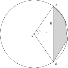
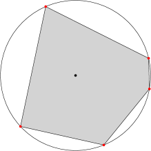
Figure 3: The eigenvalues of the unitary operator $A=U^{*}V$ (red dots, here $d=5$) and its numerical range $\mathcal{N}(A)$(gray filled area). On the left, the eigenvalues span an arc of length smaller than $\pi$, so the quantities $\nu$ and $R$ are non-trivial. On the right, the eigenvalues span an arc larger than half a circle, so the origin belongs to the numerical range; here, $\nu=0$ and $R=1$.

We consider next random unitary operators $U,V$. We analyze Haar-distributed operators and then the case where $U$ and $V$ are sampled from the distribution of two independent unitary Brownian motions stopped at different times. For independent, Haar-distributed unitary operators, in the limit of large dimension, the corresponding channels become perfectly distinguishable.

Proposition 19

Let $U,V\in\mathcal{U}(d)$ be two independent random variables, at least one of them being Haar-distributed. Then, with overwhelming probability as $d\to\infty$, the quantum channels $\Phi$ and $\Psi$ from (20) become perfectly distinguishable: for $d$ large enough,

$$\mathbb{P}\left[\|\Phi-\Psi\|_{\diamond}=2\right]\geq 1-\exp\left(-\frac{\log 2}{2}d^{2}\right).$$

Remark 20

The statement above includes the case where $U$ is a Haar-distributed random unitary matrix, and $V$ is the identity operator (hence, $\Psi$ is the identity channel).

Proof. From the hypothesis and the left / right invariance of the Haar distribution, it follows that the random matrix $W=U^{*}V$ is Haar-distributed. The estimate follows from [4, Section 3.1], where the probability of a Haar unitary matrix not having any eigenvalues in a given arc is related to a Toeplitz determinant, see equation (3.1) in [4].    

Let us now consider the case where the operators $U$ and $V$ are elements of two independent unitary Brownian motion processes. We shall not give the definition of this process, referring the reader to e.g. [8, 9, 39]. We shall only need here the following result of Biane, giving the asymptotic support of a unitary Brownian motion stopped at time $t$.

Proposition 21

[9, Proposition 10] Let $(U_{t})_{t\geq 0}$ be a unitary Brownian motion on $\mathcal{U}(d)$ starting at the identity. Then, asymtptically as $d\to\infty$, the support of the eigenvalue distribution (on the unit circle) of the operator $U_{t}$ is the full circle if $t\geq 4$ and the arc

$$\left\{\exp(i\alpha)\,:\,|\alpha|\leq\frac{1}{2}\sqrt{t(4-t)}+\arccos(1-t/2)\right\}\qquad\text{ if }0\leq t<4.$$

As a direct application of this result, we obtain the diamond norm of the difference of two unitary quantum channels stemming from independent unitary Brownian motions.

Proposition 22

Let $(U_{s})_{s\geq 0}$ and $(V_{t})_{t\geq 0}$ two independent unitary Brownian motions and consider the random unitary quantum channels $\Phi_{s}$ and $\Psi_{t}$ from (20) obtained from the operators $U_{s}$ and respectively $V_{t}$. Then, almost surely,

$$\lim_{d\to\infty}\|\Phi_{s}-\Psi_{t}\|_{\diamond}=\begin{cases}2\sin\left[\frac{1}{2}\sqrt{(s+t)(4-s-t)}+\arccos(1-(s+t)/2)\right],\quad&\text{ if }s+t<\tau\\ 2,\quad&\text{ if }s+t\geq\tau,\end{cases}$$

where $\tau\approx 0.6528$ is the unique solution of the equation

$$\frac{1}{2}\sqrt{t(4-t)}+\arccos(1-t/2)=\pi/2$$

on $(0,4)$.

Proof. The proof is an easy consequence of Biane‘s result (more precisely, of its ’’strong‘‘ formulation from [12, Theorem 1.1]), once we notice that the random unitary matrix $U_{s}^{*}V_{t}$ has the same distribution as $W_{s+t}$, where $W_{\cdot}$ is another unitary Brownian motion. We plot the diamond norm as a function of $s+t$ in Figure 4.    

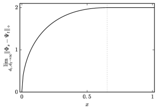
Figure 4: The diamond norm of a difference of two random unitary channels coming from two independent unitary Brownian motions stopped at times $s$ and $t$, as a function of $s+t$.

8 Concluding remarks

In this work we analyzed properties of generic quantum channels concentrating on the case of large system size. Using tools provided by the theory of random matrices and the free probability calculus we showed that the diamond norm of the difference between two random channels asymptotically tends to a constant specified in Theorem 7. In the case of channels corresponding to the simplest case $x=y=1$, the limit value of the diamond norm of the difference is $\Delta(1,1)=1/2+2/\pi$. Based on these results, in Fig. 5 we provide a sketch of the set of quantum channels. In Fig. 6 we illustrate the convergence of the upper and lower bound to the value $1/2+2/\pi$. This statement allows us to quantify the mean distinguishability between two random channels

Figure 5: Sketch of the set $\Theta(d,d)$ of all channels acting on $d$-dimensional states. A generic channel $\Phi$ belongs to a sphere of radius $r=3\sqrt{3}/2\pi$, centered at the maximally depolarizing channel, $\Phi_{\mathrm{dep}}$ in the metric induced by the diamond norm. The distance between generic channels, $\Phi,\Psi$ is $\Delta=1/2+2/\pi$, while the distance to the nearest unitary channel reads $a=2$.

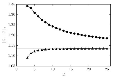
Figure 6: The convergence of upper (circles) and lower (triangles) bounds on the distance between two random quantum channels sampled from the Hilbert-Schmidt distribution ($d_{1}=d_{2}=d$). The results were obtained via Monte Carlo simulation with 100 samples for each data point.

To arrive at this result we considered an ensemble of normalized random density matrices, acting on a bipartite Hilbert space ${\mathcal{H}}_{A}\otimes{\mathcal{H}}_{B}$, and distributed according to the flat (Hilbert-Schmidt) measure. Such matrices, can be generated with help of a complex Ginibre matrix $G$ as $\rho=GG^{*}/{\rm Tr}GG^{*}$. In the simplest case of square matrices $G$ of order $d=d_{1}^{2}$ the average trace distance of a random state $\rho$ from the maximally mixed state $\rho_{*}={I}/d$ behaves asymptotically as $||\rho-\rho_{*}||_{1}\to 3\sqrt{3}/4\pi$ [38]. However, analyzing both reduced matrices $\rho_{A}={\rm Tr}_{B}\rho$ and $\rho_{B}={\rm Tr}_{A}\rho$ we can show that they become $\epsilon$ close to the maximally mixed state in sense of the operator norm, so that their smallest and largest eigenvalues do coincide. This is visualized in Fig. 7.

Figure 7: Set of all bipartite quantum states of dimension $d^{2}$, $\Omega_{d^{2}}$, (a) and its partial traces (b) and (c) containing states of dimension $d$. A generic bipartite state $\sigma_{AB}$, distant $r=3\sqrt{3}/4\pi$ from the maximally mixed state $I/d^{2}$, is mapped into $\sigma_{A}\approx\sigma_{B}\approx I/d$, while a typical pure state $|\phi_{AB}\rangle$ is sent into a generic mixed state $\rho_{A}\equiv\rho_{B}$ distant $r$ from $I/d$.

This observation implies that the state $\rho$ can be directly interpreted as a Jamiołkowski state $J$ representing a stochastic map $\Phi$, as its partial trace $\rho_{A}$ is proportional to identity. Furthermore, as it becomes asymptotically equal to the other partial trace $\rho_{B}$, it follows that a generic quantum channel (stochastic map) becomes unital and thus bistochastic.

The partial trace of a random bipartite state is shown to be close to identity provided the support of the limiting measure characterizing the bipartite state is bounded. In particular, this holds for a family of subtract Marc̆enko–Pastur distributions defined in Eq. (11) as a free additive convolution of two rescaled Marc̆enko–Pastur distributions with different parameters and determining the density of a difference of two random density matrices. In this way we could establish the upper bound for the average diamond norm between two channels and show that it asymptotically converges to the lower bound $\Delta(x,y)$ given in Theorem 10. The results obtained can be understood as an application of the measure concentration paradigm [1] to the space of quantum channels.

Acknowledgments. I.N. would like to thank Anna Jenc̆ová and David Reeb for very insightful discussion regarding the diamond norm, which led to several improvements and simplifications of the proof of Proposition 1. I.N.‘s research has been supported by the ANR projects RMTQIT ANR-12-IS01-0001-01 and StoQ ANR-14-CE25-0003-01, as well as by a von Humboldt fellowship. Financial support by the Polish National Science Centre under projects number 2016/22/E/ST6/00062 (ZP), 2015/17/B/ST6/01872 (ŁP) and 2011/02/A/ST1/00119 (KŻ) is gratefully acknowledged.

Appendix A On the partial traces of unitarily invariant random matrices

In this section we show a general result about unitarily invariant random matrices: under some technical convergence assumptions, the partial trace of a unitarily invariant random matrix is ’’flat‘‘, i.e. it is close in norm to its average.

Recall that the normalized trace functional can be extended to arbitrary permutations as follows: for a matrix $X\in M_{d}(\mathbb{C})$, write

$$\operatorname{tr}_{\pi}(X):=\prod_{c\in\pi}\frac{1}{d}\operatorname{Tr}(X^{|c|}).$$

Recall the following definition from [22, Section 4.3].

Definition 4

A sequence of random matrices $X_{d}\in M_{d}(\mathbb{C})$ is said to have almost surely limit distribution $\mu$ if

$$\forall p\geq 1,\quad\text{a.s.}-\lim_{d\to\infty}\operatorname{tr}(X^{p})=\int x^{p}d\mu(x),$$

Proposition 23

Consider a sequence of hermitian random matrices $A_{d}\in M_{d_{1}(d)}(\mathbb{C})\otimes M_{d_{2}(d)}(\mathbb{C})$ and assume that

1. Both functions $d_{1,2}(d)$ grow to infinity, in such a way that $d_{1}/d_{2}^{2}\to 0$.

2. The matrices $A_{d}$ are unitarily invariant.

3. The family $(A_{d})$ has almost surely limit distribution $\mu$, for some compactly supported probability measure $\mu$.

Then, the normalized partial traces $B_{d}:=d_{2}^{-1}[\operatorname{id}\otimes\operatorname{Tr}](A_{d})$ converge almost surely to multiple of the identity matrix:

$$\text{a.s.}-\lim_{d\to\infty}\|B_{d}-aI_{d_{1}(d)}\|=0,$$

where $a$ is the average of $\mu$:

$$a:=\int xd\mu(x).$$

Proof. In the proof, we shall drop the parameter $d\to\infty$, but the reader should remember that the matrix dimensions $d_{1,2}$ are functions of $d$ and that all the matrices appearing are indexed by $d$. To conclude, it is enough to show that

$$\mathbb{P}-\lim_{d_{1}\to\infty}\lambda_{\max}(B_{d})=a,$$

since the statement for the smallest eigenvalue follows in a similar manner. Let us denote by

$$b :=\frac{1}{d_{1}}\sum_{i=1}^{d_{1}}\lambda_{i}(B)=\operatorname{tr}_{(1)}(B)$$ (21)

$$v :=\frac{1}{d_{1}}\sum_{i=1}^{d_{1}}(\lambda_{i}(B)-b)^{2}=\frac{1}{d_{1}}\sum_{i=1}^{d_{1}}\lambda_{i}(B)^{2}-\left[\frac{1}{d_{1}}\sum_{i=1}^{d_{1}}\lambda_{i}(B)\right]^{2}=\operatorname{tr}_{(12)}(B)-[\operatorname{tr}_{(1)}(B)]^{2}$$ (22)

the average eigenvalue and, respectively, the variance of the eigenvalues of $B$; these are real random variables (actually, sequences of random variables indexed by $d$). By Chebyshev‘s inequality, we have a bound

$$\lambda_{\max}(B)\leq b+\sqrt{v}\sqrt{d_{1}}.$$ (23)

Note that one could replace the $\sqrt{d_{1}}$ factor in the inequality above by $\sqrt{d_{1}-1}$ by using Samuelson‘s inequality [40, 47], but the weaker version is enough for us.

We shall prove now that $b\to a$ almost surely and later that $d_{1}v\to 0$ almost surely, which is what we need to conclude. To do so, we shall use the Weingarten formula [48, 16]. In the graphical formalism for the Weingarten calculus introduced in [13], the expectation value of an expression involving a random Haar unitary matrix can be computed as a sum over diagrams indexed by permutation matrices; we refer the reader to [13] or [14] for the details.

Using the unitary invariance of $A$, we write $A=U\operatorname{diag}(\lambda)U^{*}$, for a Haar-distributed random unitary matrix $U\in\mathcal{U}(d_{1}d_{2})$, and some (random) eigenvalue vector $\lambda$. Note that traces of powers of $A$ depend only on $\lambda$, so we shall write $\operatorname{tr}_{\pi}(\lambda):=\operatorname{tr}_{\pi}(A)$. We apply the Weingarten formula to a general moment of $B$, given by a permutation $\pi$:

$$\mathbb{E}_{U}\operatorname{tr}_{\pi}(B)=\prod_{i=1}^{\#\pi}\frac{1}{d_{1}}\mathbb{E}_{U}\operatorname{Tr}B^{|c_{i}|},$$

where $c_{1},\ldots,c_{\#\pi}$ are the cycles of $\pi\in\mathcal{S}_{p}$, and $\mathbb{E}_{U}$ denotes the conditional expectation with respect to the Haar random unitary matrix $U$. From the graphical representation of the Weingarten formula [13, Theorem 4.1], we can compute the conditional expectation over $U$ (note that below, the vector of eigenvalues $\lambda$ is still random):

$$\mathbb{E}_{U}\operatorname{tr}_{\pi}(B)=d_{1}^{-\#\pi}d_{2}^{-p}\sum_{\alpha,\beta\in\mathcal{S}_{p}}d_{1}^{\#(\pi^{-1}\alpha)}d_{2}^{\#\alpha}(d_{1}d_{2})^{\#\beta}\operatorname{tr}_{\beta}(\lambda)\operatorname{Wg}_{d_{1}d_{2}}(\alpha^{-1}\beta).$$ (24)

Above, $\operatorname{Wg}$ is the Weingarten function [16] and $\operatorname{tr}_{\beta}(\lambda)$ is the moment of the diagonal matrix $\operatorname{diag}(\lambda)$ corresponding to the permutation $\beta$. The combinatorial factors $d_{1}^{\#(\pi^{-1}\alpha)}$ and $d_{2}^{\#\alpha}$ come from the initial wirings of the boxes respective to the vector spaces of dimensions $d_{1}$ (initial wiring given by $\pi$) and $d_{2}$ (initial wiring given by the identity permutation), see Figure 8. The pre-factors $d_{1}^{-\#\pi}d_{2}^{-p}$ contain the normalization from the (partial) traces. Finally, the (random) factors $\operatorname{tr}_{\beta}(\lambda)$ are the normalized power sums of $\lambda$:

$$\operatorname{tr}_{\beta}(\lambda)=\prod_{i=1}^{\#\beta}(d_{1}d_{2})^{-1}\sum_{j=1}^{d_{1}d_{2}}\lambda_{j}^{|w_{i}|},$$

where $w_{1},\ldots,w_{\#\beta}$ are the cycles of $\beta$. Recall that we have assumed almost sure convergence for the sequence $(A_{d})$ (and, thus, for $(\lambda_{d})$):

$$\forall\pi,\quad\text{a.s.}-\lim_{d\to\infty}\operatorname{tr}_{\beta}(\lambda)=\prod_{i=1}^{\#\beta}\int x^{|w_{i}|}d\mu(x)=:m_{\pi}(\mu).$$ (25)

Figure 8: The $i$-th group in the diagram corresponding to $m_{\pi}(B)$.

As a first application of the Weingarten formula (24), let us find the distribution of the random variable $b=\operatorname{Tr}(B)/d_{1}$. Obviously,

$$\mathbb{E}_{U}b=\mathbb{E}_{U}\operatorname{tr}_{(1)}(B)=d_{1}^{-1}d_{2}^{-1}d_{1}^{2}d_{2}^{2}\operatorname{tr}_{(1)}(\lambda)\frac{1}{d_{1}d_{2}}=\operatorname{tr}_{(1)}(\lambda).$$ (26)

Actually, $b$ does not depend on the random unitary matrix $U$, since

$$b=\frac{1}{d_{1}}\operatorname{Tr}(B)=\frac{1}{d_{1}d_{2}}\operatorname{Tr}(A)=\frac{1}{d_{1}d_{2}}\operatorname{Tr}(U\operatorname{diag}(\lambda)U^{*})=\frac{1}{d_{1}d_{2}}\sum_{i=1}^{d_{1}d_{2}}\lambda_{i}=\operatorname{tr}_{(1)}(\lambda).$$

From the hypothesis (25) (with $\pi=(1)$), we have that, almost surely as $d\to\infty$, the random variable $b$ converges to the scalar $a=m_{(1)}(\mu)$.

Let us now move on to the variance $v$ of the eigenvalues. First, we compute its expectation $\mathbb{E}_{U}v=\operatorname{tr}_{(12)}(B)-\operatorname{tr}_{(1)(2)}(B)$. We apply now the Weingarten formula (24) for $\mathbb{E}_{U}\operatorname{tr}_{(12)}(B)$; the sum has $2!^{2}=4$ terms, which we compute below:

• $\alpha=\beta=(1)(2)$: $T_{1}=d_{1}^{2}d_{2}^{2}\operatorname{tr}_{(1)(2)}(\lambda)\frac{1}{d_{1}^{2}d_{2}^{2}-1}$

• $\alpha=(1)(2)$, $\beta=(12)$: $T_{2}=-\operatorname{tr}_{(12)}(\lambda)\frac{1}{d_{1}^{2}d_{2}^{2}-1}$

• $\alpha=(12)$, $\beta=(1)(2)$: $T_{3}=-d_{1}^{2}\operatorname{tr}_{(12)}(\lambda)\frac{1}{d_{1}^{2}d_{2}^{2}-1}$

• $\alpha=\beta=(12)$: $T_{4}=d_{1}^{2}\operatorname{tr}_{(12)}(\lambda)\frac{1}{d_{1}^{2}d_{2}^{2}-1}$.

Combining the expressions above with (26), we get

$$\mathbb{E}_{U}v=\frac{d_{1}^{2}-1}{d_{1}^{2}d_{2}^{2}-1}(\operatorname{tr}_{(12)}(\lambda)-\operatorname{tr}_{(1)(2)}(\lambda)).$$

Using the hypothesis (25), we have thus, as $d_{1,2}\to\infty$,

$$\mathbb{E}v=(1+o(1))d_{2}^{-2}(m_{(12)}(\mu)-m_{(1)(2)}(\mu)).$$

Let us now proceed and estimate the variance of $v$; more precisely, let us compute $\mathbb{E}(v^{2})$. As before, we shall compute the expectation in two steps: first with respect to the random Haar unitary matrix $U$, and then, using our assumption (25), with respect to $\lambda$, in the asymptotic limit. To perform the unitary integration, note that the Weingarten sum is indexed by a couple $(\alpha,\beta)\in\mathcal{S}_{4}^{2}$, so it contains $4!^{2}=576$ terms, see [49]. In Appendix B we have computed the variance of $v$ with the usage of symmetry arguments. The result, to the first order reads

$$\operatorname{Var}(v)=\mathbb{E}_{U}(v^{2})-(\mathbb{E}_{U}v)^{2}=(1+o(1))2d_{1}^{-2}d_{2}^{-4}[m_{(12)}(\lambda)-m_{(1)(2)}(\lambda)]^{2}.$$

Taking the expectation over $\lambda$ and the limit (we are allowed to, by dominated convergence), we get

$$\operatorname{Var}(v)=(1+o(1))2d_{1}^{-2}d_{2}^{-4}[m_{(12)}(\mu)-m_{(1)(2)}(\mu)]^{2}.$$

We put now all the ingredients together:

$$\mathbb{P}(\sqrt{d_{1}}\sqrt{v}\geq\varepsilon)=\mathbb{P}(v\geq\varepsilon^{2}d_{1}^{-1})\leq\frac{\operatorname{Var}(v)}{[\varepsilon^{2}d_{1}^{-1}-\mathbb{E}v]^{2}}\sim\frac{Cd_{1}^{-2}d_{2}^{-4}}{[\varepsilon^{2}d_{1}^{-1}-(1+o(1))C^{\prime}d_{2}^{-2}]^{2}},$$

where $C,C^{\prime}$ non-negative constants depending on the limiting measure $\mu$. Using $d_{1}\ll d_{2}^{2}$, the dominating term in the denominator above is $\varepsilon^{2}d_{1}^{-1}$, and thus we have:

$$\mathbb{P}(\sqrt{d_{1}}\sqrt{v}\geq\varepsilon)\lesssim C\varepsilon^{-4}d_{2}^{-4}.$$

Since the series $\sum d_{2}^{-4}$ is summable, we obtain the announced almost sure convergence by the Borel-Cantelli lemma, finishing the proof.    

Appendix B Calculation of the variance $\operatorname{Var}(v)$

In this appendix we compute the centered second moment of the variable $v$ defined in (22) necessary to show almost sure convergence $d_{1}v\to 0$. We remind here, that $A\in M_{d_{1}}(\mathbb{C})\otimes M_{d_{2}}(\mathbb{C})$ and $B=d_{2}^{-1}[\operatorname{id}\otimes\mathrm{Tr}](A)$. Because we assume that $A$ has unitarly invariant distribution, we can write

$$A=U\mathrm{diag}(\lambda)U^{\dagger}=\sum_{i=0}^{d_{1}d_{2}-1}\lambda_{i}|U_{i}\rangle\langle U_{i}|,$$ (27)

where $|U_{i}\rangle=U|i\rangle$ is $i$-th column of matrix $U$ and

$$B=d_{2}^{-1}\mathrm{Tr}_{2}A=d_{2}^{-1}\sum_{i=0}^{d_{1}d_{2}-1}\lambda_{i}\mathrm{Tr}_{2}|U_{i}\rangle\langle U_{i}|.$$ (28)

We denote $\rho_{i}=\mathrm{Tr}_{2}|U_{i}\rangle\langle U_{i}|$ and consider mixed moments computed in Lemma 25

$$\mathcal{M}(i,j,k,l)=\mathbb{E}_{U}\mathrm{Tr}(\rho_{i}\rho_{j})\mathrm{Tr}(\rho_{k}\rho_{l}),$$ (29)

where $\mathbb{E}_{U}$ denotes the conditional expectation with respect to the Haar random unitary matrix $U$. We also define symmetric mixed moments

$$\mathcal{SM}(i,j,k,l)=\mathbb{E}_{U}\mathrm{Tr}(\rho_{i}\rho_{j})\mathrm{Tr}(\rho_{k}\rho_{l})-\mathbb{E}_{U}\mathrm{Tr}(\rho_{i}\rho_{j})\ \mathbb{E}_{U}\mathrm{Tr}(\rho_{k}\rho_{l}).$$ (30)

Proposition 24

Let $v=\frac{1}{d_{1}}\mathrm{Tr}B^{2}-\left(\frac{1}{d_{1}}\mathrm{Tr}B\right)^{2}$. Denoting $\operatorname{Var}_{U}(v)=\mathbb{E}_{U}v^{2}-(\mathbb{E}_{U}v)^{2}$, we have

$$\operatorname{Var}_{U}(v)=\frac{2(\mu_{1}^{2}-\mu_{2})^{2}}{d_{1}^{2}d_{2}^{4}}(1+o(1))$$ (31)

as $d_{1},d_{2}\to\infty$, in the above $\mu_{k}=\frac{1}{d_{1}d_{2}}\sum\lambda_{i}^{k}$.

Direct computations with the usage of symmetric moments $\mathcal{SM}$ give us

$$\begin{split}\operatorname{Var}_{U}(v)&=\frac{1}{d_{1}^{2}d_{2}^{4}}\Big{[}(d_{1}d_{2})^{4}\mu_{1}^{4}\mathcal{SM}(0,1,2,3)\\ &+2(d_{1}d_{2})^{3}\mu_{2}\mu_{1}^{2}\Big{(}\mathcal{SM}(0,0,1,2)+2\mathcal{SM}(0,1,0,2)-3\mathcal{SM}(0,1,2,3)\Big{)}\\ &+4(d_{1}d_{2})^{2}\mu_{3}\mu_{1}\Big{(}\mathcal{SM}(0,0,0,1)-\mathcal{SM}(0,0,1,2)-2\mathcal{SM}(0,1,0,2)+2\mathcal{SM}(0,1,2,3)\Big{)}\\ &+(d_{1}d_{2})^{2}\mu_{2}^{2}\Big{(}\mathcal{SM}(0,0,1,1)-2\mathcal{SM}(0,0,1,2)+2\mathcal{SM}(0,1,0,1)-4\mathcal{SM}(0,1,0,2)+3\mathcal{SM}(0,1,2,3)\Big{)}\\ &+d_{1}d_{2}\mu_{4}\Big{(}\mathcal{SM}(0,0,0,0)-4\mathcal{SM}(0,0,0,1)-\mathcal{SM}(0,0,1,1)+4\mathcal{SM}(0,0,1,2)-2\mathcal{SM}(0,1,0,1)\\ &\ \ \ \ \ \ \ \ \ \ \ \ \ \ +8\mathcal{SM}(0,1,0,2)-6\mathcal{SM}(0,1,2,3)\Big{)}\Big{]}\\ &=\frac{2\left(d_{1}^{2}-1\right)\left(d_{2}^{2}-1\right)}{d_{2}^{2}\left(d_{1}^{2}d_{2}^{2}-1\right){}^{2}\left(d_{1}^{4}d_{2}^{4}-13d_{1}^{2}d_{2}^{2}+36\right)}\Big{(}d_{1}^{4}d_{2}^{4}\left(\mu_{1}^{2}-\mu_{2}\right){}^{2}\\ &\ \ \ \ \ \ \ +d_{1}^{2}d_{2}^{2}\left(11\mu_{1}^{4}-22\mu_{2}\mu_{1}^{2}+20\mu_{3}\mu_{1}-4\mu_{2}^{2}-5\mu_{4}\right)+5\left(3\mu_{2}^{2}-4\mu_{1}\mu_{3}+\mu_{4}\right)\Big{)}.\end{split}$$ (32)

The above formula gives the exact result for $\operatorname{Var}_{U}(v)$. Considering the limiting behaviour $d_{1},d_{2}\to\infty$ we get

$$\operatorname{Var}_{U}(v)=\frac{2(\mu_{1}^{2}-\mu_{2})^{2}}{d_{1}^{2}d_{2}^{4}}(1+o(1)),$$ (33)

which completes the proof of Proposition 24.

The moments computed here are used in equation (32) to obtain the variance $\operatorname{Var}_{U}(v)$.

Lemma 25

We have the following formulas for mixed moments defined in equation (29). Note, that because of symmetry we cover all possible cases.

$$\begin{split}\mathcal{M}(0,0,0,0)&=\frac{d_{2}d_{1}^{3}+2\left(d_{2}^{2}+2\right)d_{1}^{2}+d_{2}\left(d_{2}^{2}+10\right)d_{1}+4d_{2}^{2}+2}{\left(d_{1}d_{2}+1\right)\left(d_{1}d_{2}+2\right)\left(d_{1}d_{2}+3\right)},\\ \mathcal{M}(0,0,0,1)&=\frac{\left(d_{2}^{2}-1\right)\left(d_{1}\left(d_{1}+d_{2}\right)\left(d_{1}d_{2}+4\right)+2\right)}{\left(d_{1}d_{2}-1\right)\left(d_{1}d_{2}+1\right)\left(d_{1}d_{2}+2\right)\left(d_{1}d_{2}+3\right)},\\ \mathcal{M}(0,0,1,1)&=\frac{\left(d_{1}d_{2}\left(d_{1}d_{2}+2\right)-4\right)\left(d_{1}+d_{2}\right){}^{2}+4}{d_{1}d_{2}\left(d_{1}d_{2}-1\right)\left(d_{1}d_{2}+2\right)\left(d_{1}d_{2}+3\right)},\\ \mathcal{M}(0,0,1,2)&=\frac{\left(d_{2}^{2}-1\right)\left(d_{1}\left(d_{1}+d_{2}\right)\left(d_{1}d_{2}\left(d_{1}d_{2}+4\right)+2\right)-2\right)}{d_{1}d_{2}\left(d_{1}d_{2}-1\right)\left(d_{1}d_{2}+1\right)\left(d_{1}d_{2}+2\right)\left(d_{1}d_{2}+3\right)},\\ \mathcal{M}(0,1,0,1)&=\frac{\left(d_{2}^{2}-1\right)\left(d_{1}\left(6d_{2}+d_{1}\left(d_{2}^{2}\left(d_{1}d_{2}+5\right)-2\right)\right)+2\right)}{d_{1}d_{2}\left(d_{1}d_{2}-1\right)\left(d_{1}d_{2}+1\right)\left(d_{1}d_{2}+2\right)\left(d_{1}d_{2}+3\right)},\\ \mathcal{M}(0,1,0,2)&=\frac{\left(d_{2}^{2}-1\right)\left(d_{1}\left(d_{1}\left(d_{2}\left(d_{1}\left(3d_{2}^{2}+d_{1}\left(d_{2}^{2}-1\right)d_{2}-4\right)-3d_{2}\right)+2\right)-8d_{2}\right)-2\right)}{d_{1}d_{2}\left(d_{1}d_{2}-2\right)\left(d_{1}d_{2}-1\right)\left(d_{1}d_{2}+1\right)\left(d_{1}d_{2}+2\right)\left(d_{1}d_{2}+3\right)}\\ \mathcal{M}(0,1,2,3)&=\frac{\left(d_{2}^{2}-1\right)\left(d_{2}^{2}\left(d_{2}^{2}-1\right)d_{1}^{4}+2\left(7-6d_{2}^{2}\right)d_{1}^{2}+22\right)}{d_{1}^{2}d_{2}^{2}\left(d_{1}^{2}d_{2}^{2}-7\right){}^{2}-36}.\end{split}$$ (34)

The rest of this section is devoted to the proof of the above lemma. We will omit the subscript $U$ in the expectation, because matrices $\rho_{i}$ depend only on the Haar unitary matrix $U$. Following the result of Giraud [20] we find the second moment of the purity

$$\mathcal{M}(0,0,0,0)=\mathbb{E}(\mathrm{Tr}\rho_{0}^{2})^{2}=\frac{d_{2}d_{1}^{3}+2\left(d_{2}^{2}+2\right)d_{1}^{2}+d_{2}\left(d_{2}^{2}+10\right)d_{1}+4d_{2}^{2}+2}{\left(d_{1}d_{2}+1\right)\left(d_{1}d_{2}+2\right)\left(d_{1}d_{2}+3\right)},$$ (35)

where $\rho_{0}=\mathrm{Tr}_{2}|U_{0}\rangle\langle U_{0}|$.

Next we consider the moments $\mathcal{M}(0,0,0,1)$ defined in (29)

$$\begin{split}\mathcal{M}(0,0,0,1)&=\mathbb{E}\mathrm{Tr}\rho_{0}^{2}\mathrm{Tr}(\rho_{0}\rho_{1})=\frac{1}{d_{1}d_{2}-1}\mathbb{E}\mathrm{Tr}\rho_{0}^{2}\mathrm{Tr}(\rho_{0}(d_{2}I_{d_{1}}-\rho_{0})).\end{split}$$ (36)

The above follows from the fact, that we have invariance with respect to the permutation of columns of $U$, and therefore $\mathbb{E}\mathrm{Tr}\rho_{0}^{2}\mathrm{Tr}(\rho_{0}\rho_{1})=\mathbb{E}\mathrm{Tr}\rho_{0}^{2}\mathrm{Tr}(\rho_{0}\rho_{2})$. Next we note, that $\sum_{i=0}^{d_{1}d_{2}-1}\rho_{i}=d_{2}I_{d_{1}}$. Using the above we obtain

$$\begin{split}\mathcal{M}(0,0,0,1)&=\frac{1}{d_{1}d_{2}-1}\left(d_{2}\mathbb{E}\mathrm{Tr}\rho_{0}^{2}-\mathbb{E}(\mathrm{Tr}\rho_{0}^{2})^{2}\right)\\ &=\frac{1}{d_{1}d_{2}-1}\left(d_{2}\frac{d_{1}+d_{2}}{d_{1}d_{2}+1}-\mathcal{M}(0,0,0,0)\right)\\ &=\frac{\left(d_{2}^{2}-1\right)\left(d_{1}\left(d_{1}+d_{2}\right)\left(d_{1}d_{2}+4\right)+2\right)}{\left(d_{1}d_{2}-1\right)\left(d_{1}d_{2}+1\right)\left(d_{1}d_{2}+2\right)\left(d_{1}d_{2}+3\right)}.\end{split}$$ (37)

In order to get other mixed moments we need to perform another integration. We start with expectations of the following kind

$$\mathcal{M}(0,0,1,1)=\mathbb{E}\mathrm{Tr}\rho_{0}^{2}\mathrm{Tr}\rho_{1}^{2}=\mathbb{E}\mathrm{Tr}(\mathrm{Tr}_{2}|U_{0}\rangle\langle U_{0}|)^{2}\mathrm{Tr}(\mathrm{Tr}_{2}|U_{1}\rangle\langle U_{1}|)^{2}.$$ (38)

Note that if we multiply matrix $U$ by a unitary matrix which does not change the first column we will not change the expectation value. In fact we can integrate over the subgroup of matrices which does not change the first column of $U$. Now for a moment we fix the matrix $U$ and consider the expectation value

$$\mathrm{Tr}(\mathrm{Tr}_{2}|U_{0}\rangle\langle U_{0}|)^{2}\mathbb{E}_{V}\mathrm{Tr}(\mathrm{Tr}_{2}UV|1\rangle\langle 1|V^{\dagger}U^{\dagger})^{2},$$ (39)

where matrices $V$ are in the form

$$V=\left(\begin{smallmatrix}1&0&0&\dots&0\\ 0&v_{1,1}&v_{1,2}&\dots&v_{1,d_{1}d_{2}-1}\\ 0&v_{2,1}&v_{1,2}&\dots&v_{2,d_{1}d_{2}-1}\\ \vdots&\vdots&\vdots&\ddots&\vdots\\ 0&v_{d_{1}d_{2}-1,1}&v_{d_{1}d_{2}-1,2}&\dots&v_{d_{1}d_{2}-1,d_{1}d_{2}-1}\\ \end{smallmatrix}\right).$$ (40)

The $\mathbb{E}_{V}$ is an expectation with respect to the Haar measure on $U(d_{1}d_{2}-1)$ embedded in $U(d_{1}d_{2})$, in the above way. Note, that the vector $UV|1\rangle$ represents a random orthogonal vector to the $|U_{0}\rangle=U|0\rangle$.

First we calculate

$$\begin{split}&\mathbb{E}_{V}(UV|1\rangle\langle 1|V^{\dagger}U^{\dagger})\otimes(UV|1\rangle\langle 1|V^{\dagger}U^{\dagger})\\ &=\mathbb{E}_{V}(U|V_{1}\rangle\langle V_{1}|U^{\dagger})\otimes(U|V_{1}\rangle\langle V_{1}|U^{\dagger})\\ &=(U\otimes U)\mathbb{E}_{V}|V_{1}\rangle\langle V_{1}|\otimes|V_{1}\rangle\langle V_{1}|(U\otimes U)^{\dagger}.\end{split}$$ (41)

Now, using standard integrals we obtain

$$\mathbb{E}_{V}|V_{1}\rangle\langle V_{1}|\otimes|V_{1}\rangle\langle V_{1}|=\frac{1}{(d_{1}d_{2}-1)d_{1}d_{2}}\sum_{i_{1}i_{2}j_{1}j_{2}}\left(\delta_{i_{1}j_{1}}\delta_{i_{1}j_{1}}+\delta_{i_{1}j_{2}}\delta_{i_{2}j_{1}}\right)\theta(i_{1}i_{2}j_{1}j_{2})|i_{1}i_{2}\rangle\langle j_{1}j_{2}|.$$ (42)

where $\theta(x)=(1-\delta_{x,0})$ and incorporates the condition that first element of vector $|V_{1}\rangle$ is zero. Now we obtain, after elementary calculations, using the fact that $U$ is unitary

$$\begin{split}&(U\otimes U)\mathbb{E}_{V}|V_{1}\rangle\langle V_{1}|\otimes|V_{1}\rangle\langle V_{1}|(U\otimes U)^{\dagger}\\ &=\frac{1}{(d_{1}d_{2}-1)d_{1}d_{2}}\sum_{i_{1}i_{2}j_{1}j_{2}}\Big{(}(\delta_{i_{1}j_{1}}-u_{i_{1},0}u_{j_{1},0})(\delta_{i_{2}j_{2}}-u_{i_{2},0}u_{j_{2},0})\\ &\ \ \ \ \ \ \ \ \ \ \ \ \ \ \ \ \ +(\delta_{i_{1}j_{2}}-u_{i_{1},0}u_{j_{2},0})(\delta_{i_{2}j_{1}}-u_{i_{2},0}u_{j_{1},0})\Big{)}\theta(i_{1}i_{2}j_{1}j_{2})|i_{1}i_{2}\rangle\langle j_{1}j_{2}|\\ &=\frac{1}{(d_{1}d_{2}-1)d_{1}d_{2}}\Big{(}I_{d_{1}d_{2}d_{1}d_{2}}+|U_{0}\rangle\langle U_{0}|\otimes|U_{0}\rangle\langle U_{0}|-I_{d_{1}d_{2}}\otimes|U_{0}\rangle\langle U_{0}|-|U_{0}\rangle\langle U_{0}|\otimes I_{d_{1}d_{2}}\\ &\ \ \ \ \ \ \ +S_{d_{1}d_{2}}(I_{d_{1}d_{2}d_{1}d_{2}}+|U_{0}\rangle\langle U_{0}|\otimes|U_{0}\rangle\langle U_{0}|-I_{d_{1}d_{2}}\otimes|U_{0}\rangle\langle U_{0}|-|U_{0}\rangle\langle U_{0}|\otimes I_{d_{1}d_{2}})\Big{)},\end{split}$$ (43)

where $S_{N}$ is a swap operation on two systems of dimensions $N$ each, i.e. $S=\sum_{i_{1},i_{2}=0}^{N-1}|i_{1}i_{2}\rangle\langle i_{2}i_{1}|$. So we get

$$\begin{split}&(U\otimes U)\mathbb{E}_{V}|V_{1}\rangle\langle V_{1}|\otimes|V_{1}\rangle\langle V_{1}|(U\otimes U)^{\dagger}\\ &=\frac{1}{(d_{1}d_{2}-1)d_{1}d_{2}}(I_{d_{1}d_{2}d_{1}d_{2}}+S_{d_{1}d_{2}})\Big{(}I_{d_{1}d_{2}}+|U_{0}\rangle\langle U_{0}|\otimes|U_{0}\rangle\langle U_{0}|-I_{d_{1}d_{2}}\otimes|U_{0}\rangle\langle U_{0}|-|U_{0}\rangle\langle U_{0}|\otimes I_{d_{1}d_{2}}\Big{)},\end{split}$$ (44)

We are going to use several times the following identity often used in quantum information. For two square matrices $\rho_{1},\rho_{2}$ of size $N$

$$\mathrm{Tr}\rho_{1}\rho_{2}=\mathrm{Tr}S_{N}(\rho_{1}\otimes\rho_{2}).$$ (45)

This identity allows us to obtain

$$\begin{split}&\mathbb{E}_{V}\mathrm{Tr}(\mathrm{Tr}_{2}U|V_{1}\rangle\langle V_{1}|U^{\dagger})^{2}=\mathbb{E}\mathrm{Tr}S_{d_{1}}(\mathrm{Tr}_{2}U|V_{1}\rangle\langle V_{1}|U^{\dagger})\otimes(\mathrm{Tr}_{2}U|V_{1}\rangle\langle V_{1}|U^{\dagger})\\ &=\mathbb{E}_{V}\mathrm{Tr}S_{d_{1}}\mathrm{Tr}_{2,4}(U|V_{1}\rangle\langle V_{1}|U^{\dagger}\otimes U|V_{1}\rangle\langle V_{1}|U^{\dagger})\\ &=\mathrm{Tr}S_{d_{1}}\mathrm{Tr}_{2,4}(U\otimes U)\mathbb{E}_{V}|V_{1}\rangle\langle V_{1}|\otimes|V_{1}\rangle\langle V_{1}|(U\otimes U)^{\dagger}\\ &=\frac{1}{(d_{1}d_{2}-1)d_{1}d_{2}}\mathrm{Tr}S_{d_{1}}\mathrm{Tr}_{2,4}(I_{d_{1}d_{2}d_{1}d_{2}}+S_{d_{1}d_{2}})\Big{(}I_{d_{1}d_{2}d_{1}d_{2}}+|U_{0}\rangle\langle U_{0}|\otimes|U_{0}\rangle\langle U_{0}|\\ &\ \ \ \ \ -I_{d_{1}d_{2}}\otimes|U_{0}\rangle\langle U_{0}|-|U_{0}\rangle\langle U_{0}|\otimes I_{d_{1}d_{2}}\Big{)}.\end{split}$$ (46)

After performing partial trace over subsystems 2 and 4 we get

$$\begin{split}&\mathbb{E}_{V}\mathrm{Tr}(\mathrm{Tr}_{2}U|V_{1}\rangle\langle V_{1}|U^{\dagger})^{2}\\ &=\frac{1}{(d_{1}d_{2}-1)d_{1}d_{2}}\Big{(}d_{1}d_{2}^{2}+\mathrm{Tr}\rho_{0}^{2}-d_{2}\mathrm{Tr}\rho_{0}-d_{2}\mathrm{Tr}\rho_{0}+d_{1}^{2}d_{2}+\mathrm{Tr}(\rho^{\prime}_{0})^{2}-d_{1}\mathrm{Tr}\rho^{\prime}_{0}-d_{1}\mathrm{Tr}\rho^{\prime}_{0}\Big{)}\\ &=\frac{1}{(d_{1}d_{2}-1)d_{1}d_{2}}\Big{(}d_{1}d_{2}^{2}+d_{1}^{2}d_{2}-2d_{1}-2d_{2}+2\mathrm{Tr}\rho_{0}^{2}\Big{)}.\end{split}$$ (47)

In the above formulas we used $\rho^{\prime}_{0}=\mathrm{Tr}_{1}|U_{0}\rangle\langle U_{0}|$ and the fact, that two partial traces of a pure bi-partite state have the same purity $\mathrm{Tr}\rho_{0}^{2}=\mathrm{Tr}(\rho^{\prime}_{0})^{2}$. Using the above we find the desired expectation

$$\begin{split}\mathcal{M}(0,0,1,1)&=\mathbb{E}\mathrm{Tr}\rho_{0}^{2}\mathrm{Tr}\rho_{1}^{2}=\mathbb{E}\mathrm{Tr}\rho_{0}^{2}\mathbb{E}_{V}\mathrm{Tr}(\mathrm{Tr}_{2}U|V_{1}\rangle\langle V_{1}|U^{\dagger})^{2}\\ &=\frac{1}{(d_{1}d_{2}-1)d_{1}d_{2}}\Big{(}(d_{1}d_{2}^{2}+d_{1}^{2}d_{2}-2d_{1}-2d_{2})\mathbb{E}\mathrm{Tr}\rho_{0}^{2}+2\mathbb{E}(\mathrm{Tr}\rho_{0}^{2})^{2}\Big{)}\\ &=\frac{1}{(d_{1}d_{2}-1)d_{1}d_{2}}\Big{(}(d_{1}d_{2}^{2}+d_{1}^{2}d_{2}-2d_{1}-2d_{2})\frac{d_{1}+d_{2}}{d_{1}d_{2}+1}+2\mathcal{M}(0,0,0,0)\Big{)}\\ &=\frac{\left(d_{1}d_{2}\left(d_{1}d_{2}+2\right)-4\right)\left(d_{1}+d_{2}\right){}^{2}+4}{d_{1}d_{2}\left(d_{1}d_{2}-1\right)\left(d_{1}d_{2}+2\right)\left(d_{1}d_{2}+3\right)}.\end{split}$$ (48)

Using inner integral we can also calculate the other mixed moments

$$\begin{split}&\mathcal{M}(0,1,0,1)=\mathbb{E}\mathrm{Tr}\rho_{0}\rho_{1}\mathrm{Tr}\rho_{0}\rho_{1}=\mathbb{E}\mathrm{Tr}(\rho_{0}\otimes\rho_{0})(\rho_{1}\otimes\rho_{1})\\ &=\mathbb{E}\mathrm{Tr}(\rho_{0}\otimes\rho_{0})\mathrm{Tr}_{2,4}(U\otimes U)\mathbb{E}_{V}|V_{1}\rangle\langle V_{1}|\otimes|V_{1}\rangle\langle V_{1}|(U\otimes U)^{\dagger}\\ &=\frac{1}{(d_{1}d_{2}-1)d_{1}d_{2}}\mathbb{E}\mathrm{Tr}(\rho_{0}\otimes\rho_{0})\mathrm{Tr}_{2,4}(I_{d_{1}d_{2}d_{1}d_{2}}+S_{d_{1}d_{2},d_{1}d_{2}})\\ &\ \ \ \times\Big{(}I_{d_{1}d_{2}d_{1}d_{2}}+|U_{0}\rangle\langle U_{0}|\otimes|U_{0}\rangle\langle U_{0}|-I_{d_{1}d_{2}}\otimes|U_{0}\rangle\langle U_{0}|-|U_{0}\rangle\langle U_{0}|\otimes I_{d_{1}d_{2}}\Big{)}\\ &=\frac{1}{(d_{1}d_{2}-1)d_{1}d_{2}}\mathbb{E}\Big{(}\mathrm{Tr}(\rho_{0}\otimes\rho_{0})(d_{2}^{2}I_{d_{1}^{2}}+\rho_{0}\otimes\rho_{0}-d_{2}I_{d_{1}}\otimes\rho_{0}-d_{2}\rho_{0}\otimes I_{d_{2}})\\ &+\mathrm{Tr}S_{d_{1}d_{2},d_{1}d_{2}}\Big{(}I_{d_{1}d_{2}d_{1}d_{2}}+|U_{0}\rangle\langle U_{0}|\otimes|U_{0}\rangle\langle U_{0}|-I_{d_{1}d_{2}}\otimes|U_{0}\rangle\langle U_{0}|-|U_{0}\rangle\langle U_{0}|\otimes I_{d_{1}d_{2}}\Big{)}(\rho_{0}\otimes I_{d_{2}}\otimes\rho_{0}\otimes I_{d_{2}})\Big{)}\\ &=\frac{1}{(d_{1}d_{2}-1)d_{1}d_{2}}\mathbb{E}\Big{(}d_{2}^{2}+(\mathrm{Tr}\rho_{0}^{2})^{2}-2d_{2}\mathrm{Tr}\rho_{0}\mathrm{Tr}\rho_{0}^{2}\\ &+\mathrm{Tr}(\rho_{0}^{2}\otimes I_{d_{2}})+\mathrm{Tr}(|U_{0}\rangle\langle U_{0}|\rho_{0}\otimes I_{d_{2}})^{2}-2\mathrm{Tr}(\rho_{0}\otimes I_{d_{2}})(|U_{0}\rangle\langle U_{0}|\rho_{0}\otimes I_{d_{2}})\Big{)}\\ &=\frac{1}{(d_{1}d_{2}-1)d_{1}d_{2}}\mathbb{E}\Big{(}d_{2}^{2}-2d_{2}\mathrm{Tr}\rho_{0}^{2}+(\mathrm{Tr}\rho_{0}^{2})^{2}+d_{2}\mathrm{Tr}\rho_{0}^{2}+(\mathrm{Tr}\rho_{0}^{2})^{2}-2\mathrm{Tr}\rho_{0}^{3}\Big{)}\\ &=\frac{1}{(d_{1}d_{2}-1)d_{1}d_{2}}\Big{(}d_{2}^{2}-d_{2}\frac{d_{1}+d_{2}}{d_{1}d_{2}+1}+2\mathcal{M}(0,0,0,0)-2\mathbb{E}\mathrm{Tr}\rho_{0}^{3}\Big{)}\\ &=\frac{\left(d_{2}^{2}-1\right)\left(d_{1}\left(6d_{2}+d_{1}\left(d_{2}^{2}\left(d_{1}d_{2}+5\right)-2\right)\right)+2\right)}{d_{1}d_{2}\left(d_{1}d_{2}-1\right)\left(d_{1}d_{2}+1\right)\left(d_{1}d_{2}+2\right)\left(d_{1}d_{2}+3\right)}.\end{split}$$ (49)

This is because $\mathbb{E}\mathrm{Tr}\rho_{0}^{3}=\frac{\left(d_{1}+d_{2}\right){}^{2}+d_{1}d_{2}+1}{\left(d_{1}d_{2}+1\right)\left(d_{1}d_{2}+2\right)}$ see [41].

Using above results we obtain other moments

$$\begin{split}\mathcal{M}(0,0,1,2)&=\mathbb{E}\mathrm{Tr}\rho_{0}^{2}\mathrm{Tr}(\rho_{1}\rho_{2})=\frac{1}{d_{1}d_{2}-2}\mathbb{E}\mathrm{Tr}\rho_{0}^{2}\mathrm{Tr}(\rho_{1}(d_{2}I_{d_{1}}-\rho_{0}-\rho_{1}))\\ &=\frac{1}{d_{1}d_{2}-2}\left(d_{2}\mathbb{E}\mathrm{Tr}\rho_{0}^{2}-\mathbb{E}\mathrm{Tr}\rho_{0}^{2}\mathrm{Tr}(\rho_{1}\rho_{0})-\mathbb{E}\mathrm{Tr}\rho_{0}^{2}\mathrm{Tr}\rho_{1}^{2}\right)\\ &=\frac{1}{d_{1}d_{2}-2}\left(d_{2}\frac{d_{1}+d_{2}}{d_{1}d_{2}+1}-\mathcal{M}(0,0,0,1)-\mathcal{M}(0,0,1,1)\right)\\ &=\frac{\left(d_{2}^{2}-1\right)\left(d_{1}\left(d_{1}+d_{2}\right)\left(d_{1}d_{2}\left(d_{1}d_{2}+4\right)+2\right)-2\right)}{d_{1}d_{2}\left(d_{1}d_{2}-1\right)\left(d_{1}d_{2}+1\right)\left(d_{1}d_{2}+2\right)\left(d_{1}d_{2}+3\right)}.\end{split}$$ (50)

Next we consider the mixed moment of type $(0,1,0,2)$,

$$\begin{split}\mathcal{M}(0,1,0,2)&=\mathbb{E}\mathrm{Tr}(\rho_{0}\rho_{1})\mathrm{Tr}(\rho_{0}\rho_{2})=\frac{1}{d_{1}d_{2}-2}\mathbb{E}\mathrm{Tr}(\rho_{0}\rho_{1})\mathrm{Tr}(\rho_{0}(d_{2}I_{d_{1}}-\rho_{0}-\rho_{1}))\\ &=\frac{1}{d_{1}d_{2}-2}\left(d_{2}\mathbb{E}\mathrm{Tr}(\rho_{0}\rho_{1})-\mathbb{E}\mathrm{Tr}(\rho_{0}\rho_{1})\mathrm{Tr}(\rho_{0}^{2})-\mathbb{E}\mathrm{Tr}(\rho_{0}\rho_{1})\mathrm{Tr}(\rho_{0}\rho_{1})\right)\\ &=\frac{\left(d_{2}^{2}-1\right)\left(d_{1}\left(d_{1}\left(d_{2}\left(d_{1}\left(3d_{2}^{2}+d_{1}\left(d_{2}^{2}-1\right)d_{2}-4\right)-3d_{2}\right)+2\right)-8d_{2}\right)-2\right)}{d_{1}d_{2}\left(d_{1}d_{2}-2\right)\left(d_{1}d_{2}-1\right)\left(d_{1}d_{2}+1\right)\left(d_{1}d_{2}+2\right)\left(d_{1}d_{2}+3\right)}.\end{split}$$ (51)

Consider now the last case of all different indices

$$\begin{split}\mathcal{M}(0,1,2,3)&=\mathbb{E}\mathrm{Tr}(\rho_{0}\rho_{1})\mathrm{Tr}(\rho_{2}\rho_{3})\\ &=\frac{1}{d_{1}d_{2}-3}\mathbb{E}\mathrm{Tr}(\rho_{0}\rho_{1})\mathrm{Tr}(\rho_{2}(d_{2}I_{d_{1}}-\rho_{0}-\rho_{1}-\rho_{2})\\ &=\frac{1}{d_{1}d_{2}-3}\mathbb{E}\mathrm{Tr}(\rho_{0}\rho_{1})\left(d_{2}-\mathrm{Tr}\rho_{2}\rho_{0}-\mathrm{Tr}\rho_{2}\rho_{1}-\mathrm{Tr}\rho_{2}\rho_{2}\right)\\ &=\frac{\left(d_{2}^{2}-1\right)\left(d_{2}^{2}\left(d_{2}^{2}-1\right)d_{1}^{4}+2\left(7-6d_{2}^{2}\right)d_{1}^{2}+22\right)}{d_{1}^{2}d_{2}^{2}\left(d_{1}^{2}d_{2}^{2}-7\right){}^{2}-36}.\end{split}$$ (52)

In this way we calculated all the moments defined in eqn. (29). Symmetrizing them according the eqn. (30) they can be used in eqn. (32) to establish Proposition 24.

References

• [1] Aubrun, G., Szarek, S. Alice and Bob meet Banach. Book in preparation.
• [2] Bai, Z. and Silverstein, J. W. Spectral Analysis of Large Dimensional Random Matrices. Springer Series in Statistics, 2010.
• [3] Bai, Z. D. and Yin Y. Q. Limit of the smallest eigenvalue of large dimensional covariance matrix. The Annals of Probability, 21, 1275–1294, 1993.
• [4] Ben Arous, G., Bourgade, P. Extreme gaps between eigenvalues of random matrices. The Annals of Probability, 41, 2648–2681, 2013.
• [5] Bercovici, H. and Voiculescu, D. Regularity questions for free convolution. Operator Theory, 104, 37–47, 1998.
• [6] Bhatia, R. Matrix Analysis. Graduate Texts in Mathematics, 169. Springer-Verlag, New York, 1997.
• [7] Bhatia, R. Matrix factorizations and their perturbations. Linear Algebra and its Applications 197, 245–276, 1994.
• [8] Biane, P. Free Brownian motion, free stochastic calculus and random matrices. In Free probability theory (Waterloo, ON, 1995), vol. 12 of Fields Institute Communications, American Mathematical Society, Providence, 1997, 1–19.
• [9] Biane, P. Segal-Bargmann transform, functional calculus on matrix spaces and the theory of semi-circular and circular systems. Journal of Functional Analysis, 144, 232–286, 1997.
• [10] W. Bruzda, V. Cappellini, H-J. Sommers, K. Życzkowski Random quantum operations Physics Letters A, 373, 320–324, 2009.
• [11] Choi, M.-D. Completely positive linear maps on complex matrices. Linear Algebra and its Applications, 10, 285, 1975.
• [12] Collins, B., Dahlqvist, A., Kemp, T. Strong Convergence of Unitary Brownian Motion. Preprint arXiv:1502.06186.
• [13] Collins, B. and Nechita, I. Random quantum channels I: Graphical calculus and the Bell state phenomenon. Communications in Mathematical Physics, 297, 345–370, 2010.
• [14] Collins, B. and Nechita, I. Random matrix techniques in quantum information theory. Journal of Mathematical Physics 57, 015215, 2016.
• [15] Collins, B., Nechita, I. and Ye, D. The absolute positive partial transpose property for random induced states. Random Matrices: Theory and Applications. 01, 1250002, 2012.
• [16] Collins, B. and Śniady, P. Integration with respect to the Haar measure on unitary, orthogonal and symplectic group. Communications in Mathematical Physics, 264, 773–795, 2006.
• [17] Davies, E.B. Lipschitz continuity of operators in the Schatten classes. Journal of the London Mathematical Society, 37, 148–157, 1988.
• [18] Deya, A., Nourdin, I. Convergence of Wigner integrals to the tetilla law. Latin American Journal of Probability and Mathematical Statistics, 9, 101–127, 2012.
• [19] Fuchs, C.A. and Van De Graaf, J. Cryptographic distinguishability measures for quantum-mechanical states, IEEE Transactions on Information Theory, 45(4), 1216–1227, 1999
• [20] Giraud, O. Distribution of bipartite entanglement for random pure states, Journal of Physics A: Mathematical and Theoretical, 40, 2793, 2007.
• [21] Helstrom, C. W. Quantum detection and estimation theory. Academic press, 1976
• [22] Hiai, F., and Petz, D. The semicircle law, free random variables, and entropy. AMS, 2000.
• [23] Holevo, A. S. An analogue of statistical decision theory and noncommutative probability theory. Trudy Moskovskogo Matematicheskogo Obshchestva, 26, 133–149, 1972.
• [24] Horn, R. and Johnson, C. Topics in matrix analysis. Cambridge University Press, 1991.
• [25] Kitaev, A. Y. Quantum computations: algorithms and error correction. Russian Mathematical Surveys 52, 1191–1249, 1997.
• [26] Jamiołkowski, A. Linear transformations which preserve trace and positive semidefiniteness of operators. Reports on Mathematical Physics, 3, 275–278, 1972.
• [27] Jenc̆ová, A. and Plávala, M. Conditions for optimal input states for discrimination of quantum channels. Journal of Mathematical Physics, 57, 122203, 2016.
• [28] Johnston, N., Kribs, D., Paulsen, V. Computing stabilized norms for quantum operations via the theory of completely bounded maps. Quantum Information and Computation, 9, 0016–0035, 2009.
• [29] Johnston, N. QETLAB: A MATLAB toolbox for quantum entanglement, version 0.9. http://www.qetlab.com, January 12, 2016.
• [30] Kliesch, M., Kueng, R., Eisert, J., Gross, D. Improving compressed sensing with the diamond norm. IEEE Transactions on Information Theory, 62, 7445–7463, 2016.
• [31] Male, C. The norm of polynomials in large random and deterministic matrices. Probability Theory and Related Fields, 154, 477–532, 2012.
• [32] Michel, U., Kliesch, M., Kueng, R., Gross, D. Note on the saturation of the norm inequalities between diamond and nuclear norm. Preprint arXiv:1612.07931.
• [33] Nica, A. and Speicher, R. Lectures on the combinatorics of free probability. Cambridge University Press (2006).
• [34] Nica, A., Speicher, R. Commutators of free random variables. Duke Mathematical Journal, 92, 553–592, 1998.
• [35] Paulsen, V. Completely bounded maps and operator algebras. Cambridge University Press (2002).
• [36] Popescu, S. and Short, A. J. and Winter, A. Entanglement and the foundations of statistical mechanics. Nature Physics, 2, 754–758, 2006.
• [37] Puchała, Z. and Jenčová, A. and Sedlák, M. and Ziman, M., Exploring boundaries of quantum convex structures: Special role of unitary processes, Physical Review A, 92(1), 012304, 2015.
• [38] Puchała, Z., Pawela, Ł., Życzkowski, K. Distinguishability of generic quantum states. Physical Review A, 93, 062112, 2016.
• [39] Rains, E. M. Combinatorial properties of Brownian motion on the compact classical groups. Journal of Theoretical Probability, 10, 659–679, 1997.
• [40] Samuelson, P. A. How deviant can you be? Journal of the American Statistical Association, 63, 1522–1525, 1968.
• [41] Sommers, H.-J. and Życzkowski, K. Statistical properties of random density matrices, J. Phys. A: Math. Gen., 37. 8457, 2004.
• [42] Stinespring, W. F. Positive functions on $C^{*}$-algebras. Proceedings of the American Mathematical Society, 6, 211–216, 1955.
• [43] S. Szarek, E. Werner, K. Życzkowski, Geometry of sets of quantum maps: a generic positive map acting on a high-dimensional system is not completely positive Journal of Mathematical Physics, 49, 032113, 2008.
• [44] Timoney, R. M. Computing the norms of elementary operators. Illinois Journal of Mathematics, 47, 1207–1226, 2003.
• [45] Watrous, J. Theory of Quantum Information. Book draft available at https://cs.uwaterloo.ca/~watrous/TQI/, 2016.
• [46] Watrous, J. Simpler semidefinite programs for completely bounded norms. Chicago Journal of Theoretical Computer Science, 8, 1–19, 2013.
• [47] Wolkowicz, H. and Styan, G.P.H., Bounds for eigenvalues using traces, Linear Algebra and Its Applications, 29, 471–506, 1980.
• [48] Weingarten, D. Asymptotic behavior of group integrals in the limit of infinite rank. Journal of Mathematical Physics, 19, 999–1001, 1978.
• [49] A Mathematica notebook can be found in the supplementary material of the current paper.