Statistics and structure of spanwise rotating turbulent channel flow at moderate Reynolds numbers

Abstract

A study of fully developed plane turbulent channel flow subject to spanwise system rotation through direct numerical simulations is presented. In order to study both the influence of the Reynolds number and spanwise rotation on channel flow, the Reynolds number $Re=U_{b}h/\nu$ is varied from a low 3000 to a moderate $31\,600$ and the rotation number $Ro=2\Omega h/U_{b}$ is varied from 0 to 2.7, where $U_{b}$ is the mean bulk velocity, $h$ the channel half gap and $\Omega$ the system rotation rate. The mean streamwise velocity profile displays also at higher $Re$ the characteristic linear part with a slope near to $2\Omega$ and a corresponding linear part in the profiles of the production and dissipation rate of turbulent kinetic energy appears. With increasing $Ro$ a distinct unstable side with large spanwise and wall-normal Reynolds stresses and a stable side with much weaker turbulence develops in the channel. The flow starts to relaminarize on the stable side of the channel and persisting turbulent-laminar patterns appear at higher $Re$. If $Ro$ is further increased the flow on the stable side becomes laminar-like while at yet higher $Ro$ the whole flow relaminarizes, although the calm periods might be disrupted by repeating bursts of turbulence, as explained by Brethouwer (2016). The influence of the Reynolds number is considerable, in particular on the stable side of the channel where velocity fluctuations are stronger and the flow relaminarizes less quickly at higher $Re$. Visualizations and statistics show that at $Ro=0.15$ and 0.45 large-scale structures and large counter rotating streamwise roll cells develop on the unstable side. These become less noticeable and eventually vanish when $Ro$ raises, especially at higher $Re$. At high $Ro$, the largest energetic structures are larger at lower $Re$.

I Introduction

Turbulent plane channel flow subject to rotation about the spanwise direction displays several phenomena of interest to engineering applications, turbulence modelling (Jakirlić et al. 2002, Smirnov & Menter 2009, Arolla & Durbin 2013, Hsieh et al. 2016) and subgrid-scale modelling in large-eddy simulation (Marstorp et al. 2009, Yang et al. 2012). Effects of rotation on flow and turbulence are in this case non-trivial. Channel flow is unaffected by rotation if fluid motions are two-dimensional and perpendicular to the rotation axis (Tritton 1992), for example, laminar Poiseuille flow and waves perpendicular to the rotation axis are not influenced (Brethouwer et al. 2014). Yet, it is well-established that spanwise rotation strongly influences Reynolds stresses, anisotropy and structures, and the mean velocity profile in plane turbulent channel flow (Johnston et al. 1972). Rotation effects are therefore obviously related to three-dimensional turbulent processes.

A useful parameter when discussing rotation effects on turbulent shear flows is the ratio of background and mean shear vorticity. For a unidirectional shear flow with mean velocity $U(y)$ in the $x$-direction and shear vorticity $-\mbox{d}U/\mbox{d}y$ rotating with angular velocity $\Omega$ about the $z$-axis, this ratio is given by

$$S=-\frac{2\Omega}{\mbox{d}U/\mbox{d}y}.$$ (1)

When $S>0$ the mean shear and background vorticity have the same sense of rotation and rotation is cyclonic and when $S<0$ they have the opposite sense and rotation is anti-cyclonic. Displaced particle analysis (Tritton 1992), rapid distortion theory, large-eddy and direct numerical simulation (DNS) of rotating homogeneous turbulent shear flow demonstrate that turbulence is damped if $S>0$ and $S<-1$ and augmented if $-1<S<0$ (Salhi & Cambon 1997, Brethouwer 2005).

Experiments of fully developed turbulent plane channel flow subject to spanwise rotation by Johnston et al. (1972) at $Re=U_{b}h/\nu=5750$, $Ro=2\Omega h/U_{b}\leq 0.21$ and $Re=17500$, $Ro\leq 0.081$, and by Nakabayashi & Kitoh (2005) at $Re\leq 2750$ and $Ro\leq 0.056$, where $U_{b}$ is the bulk mean velocity, $h$ channel half-width, $\nu$ viscosity and $\Omega$ rotation rate, have shown that turbulence is suppressed on one side of the channel where $S>0$ and augmented on the other side where $-1<S<0$, in accordance with the discussion above. These sides are from now on called the stable and unstable side, respectively.

DNS of spanwise rotating channel flow have been carried out by Kristoffersen & Andersson (1993) at $Re_{\tau}=194$ and $Ro\leq 0.5$, Lamballais et al. (1996) at $Re=2500$ and $Ro\leq 1.5$, Nagano & Hattori (2003) at $Re_{\tau}=150$ and $Ro_{\tau}\leq 5$ corresponding to $Ro\lesssim 0.3$, and Liu & Lu (2006) at $Re_{\tau}=194$ and $Ro_{\tau}\leq 7.5$ corresponding to $Ro\lesssim 0.5$. Here, $Re_{\tau}$ and $Ro_{\tau}$ are based on the friction velocity instead of $U_{b}$. Yang et al. (2012) have performed DNSs of rotating channel flow at $Re=7000$ and $Ro\leq 0.6$ to validate their large-eddy simulations. These DNSs were broadly consistent with the experimental observations and show that at sufficiently high $Ro$ the flow becomes laminar-like on the stable side owing to the strong suppression of turbulence. The asymmetry of the Reynolds stresses induces a skewed mean velocity profile and differences in the shear stresses on the two walls. Another notable feature is the appearance of a region in the channel where the mean velocity profile is linear with a slope $\mbox{d}U/\mbox{d}y\approx 2\Omega$, i.e. $S\approx-1$, implying that the absolute mean vorticity is nearly zero. Spanwise rotation affects turbulence anisotropy too since wall-normal fluctuations are typically strongly augmented on the unstable side (Kristoffersen & Andersson 1993), again in line with DNS of rotating homogeneous shear flow (Brethouwer 2005). Another consequence of spanwise system rotation is the emergence of large streamwise roll cells at certain $Ro$ induced by the Coriolis force, as shown by experiments and DNS (Johnston et al. 1972, Kristoffersen & Andersson 1993, Dai et al. 2016).

Higher $Ro$ was considered by Grundestam et al. (2008), who have performed DNS of spanwise rotating channel flow at $Re_{\tau}=180$ and $Ro\leq 2.49$. Besides one-point statistics, they studied the effect of rotation on turbulent structures and Reynolds stress budgets. They observed that at higher $Ro$ turbulence was weak as well on the unstable side, suggesting that the flow fully relaminarizes at sufficiently high $Ro$. This can be understood from the fact that in Poiseuille flow $S\geq 0$ and $S\leq-1$ everywhere in the channel if $Ro\geq 3.0$. A more rigorous stability analysis shows that all modes with spanwise wavenumber $\beta\neq 0$ are linearly stable for $Ro>Ro_{c}$ in plane Poiseuille flow with spanwise rotation (Wallin et al. 2013). The critical rotation number $Ro_{c}$ is a monotonic function of $Re$, i.e. $Ro_{c}=2.80$ for $Re=10000$ and $Ro_{c}\rightarrow 3.0$ for $Re\rightarrow\infty$. DNS confirms that the flow relaminarizes when $Ro\rightarrow Ro_{c}$ (Wallin et al. 2013).

However, Tollmien-Schlichting (TS) waves with a wave vector normal to the rotation axis are unaffected by spanwise rotation and become linearly unstable in plane Poiseuille flow if $Re\geq 3848$ (Schmid & Henningson 2001). DNS indeed reveal TS wave instabilities resulting in a continuous cycle of turbulent bursts if $Ro\simeq Ro_{c}$ and the flow is basically laminar (Wallin et al. 2013). Absence of turbulence though is not a prerequisite for TS instabilities, as shown by Brethouwer et al. (2014) who have observed cyclic bursts of intense turbulence triggered by an unstable TS wave in DNS at $Re=20000$ and $Ro=1.2$ when turbulence is strong on the unstable side. An extensive study of DNSs of spanwise rotating channel flow reveals that these cyclic turbulent bursts and TS wave instabilities show up in a quite wide range of $Re$ and $Ro$ including cases with overall weak turbulence as well as strong continuous turbulence on the unstable side (Brethouwer 2016). The observed TS instability growth was compared with linear stability theory predictions and analyzed in detail.

DNSs at $Re_{\tau}=180$ and a wide range of $Ro$ were also performed by Xia et al. (2016). They studied various one-point statistics and observed a linear part in the profile of the streamwise Reynolds stress production at sufficiently high $Ro$. Another study of spanwise rotating channel flow was performed by Yang & Wu (2012) who have carried out DNSs at $Re_{\tau}=180$ and performed a helical wave decomposition. This shows that at low $Ro$ energy concentrates in large-scale modes, presumably streamwise roll cells, while at higher $Ro$ energy accumulates at smaller scales. In DNSs with periodic boundary conditions these roll cells appear as pairs of counter-rotating vortices. Dai et al. (2016) have detected roll cells, sometimes called Taylor-Görtler vortices, in DNS at $Re=2800$ and $0.1\leq Ro\leq 0.5$ and $Re=7000$ and $Ro=0.3$, and studied their effect on the turbulence. They found that, somewhat counter intuitively, turbulence is enhanced on the unstable side in the low-wall-shear-stress region where the fluid is pumped away from the wall by the counter-rotating roll cells. Hsieh & Biringen have carried out DNSs of rotating channel flow at $Re_{\tau}\approx 200$ with $0\leq Ro\leq 0.5$ and $Re_{\tau}\approx 400$ with $Ro=0.2$ with varying domain sizes. At low $Re_{\tau}$ they observed that when the spanwise domain was too small to capture a full pair of counter-rotating roll cells the mean velocity profiles and Reynolds stresses were incorrect, illustrating that the roll cells have a significant impact on the momentum transfer and turbulence. At higher $Re_{\tau}$ the mean velocity and Reynolds stresses changed significantly when the spanwise domain size was reduced from $2\pi h$ to $\pi h$.

These previous studies of spanwise rotating channel flow were mostly limited to low Reynolds numbers, $Re_{\tau}\leq 194$, meaning that the influence of the Reynolds number on the statistics, turbulent structures and relaminarization on the stable side can be significant. Exceptions are the experiments of Johnston et al. (1972) and DNSs of Dai et al. (2016) and Hsieh & Biringen (2016) at somewhat higher $Re$ albeit limited to moderate $Ro$. It is therefore not completely clear if the previous observations have been influenced by the low $Re$. I have carried out DNSs of plane turbulent channel flow subject to spanwise rotation at higher Reynolds numbers than in previous studies with $Re$ up to $31\,600$ and a wide range of $Ro$. My aim is to assess the influence of spanwise rotation on the mean velocity, one-point statistics and Reynolds stress budgets at these higher $Re$. With these simulations I will investigate whether the effects of rotation on the mean flow and turbulence discussed above are either generic or influenced by the Reynolds number. Another goal is to study the relaminarization of the flow on the stable channel side at high $Ro$ and turbulence structures, and examine if roll cells exist in rotating channel flow at these higher $Re$. Some previous observations of the flow structures and relaminarization may have been affected by the limited computational domains that were often used in the numerical studies. In the present study, I therefore use larger computational domains and study the structures through visualizations, two-point correlations and spectra. Finally, the effect of $Re$ on the flow statistics and structures is studied at a fixed $Ro$. The present study is also motivated by the need for higher $Re$ data of rotating channel flow for turbulence modelling.

II Numerical method and parameters

The velocity $\mathbf{u}$ in the DNSs is governed by the incompressible Navier-Stokes equations

$$\frac{\partial\mathbf{u}}{\partial t}+\mathbf{u}\mathbf{\cdot}\mathbf{\nabla}\mathbf{u}=-\mathbf{\nabla}p+\frac{1}{Re}\nabla^{2}\mathbf{u}-Ro(\mathbf{e}_{z}\times\mathbf{u}),~{}~{}~{}\mathbf{\nabla}\mathbf{\cdot}\mathbf{u}=0,$$ (2)

where $\mathbf{e}_{z}$ is the unit vector in the $z$-direction and $p$ the pressure including the centrifugal acceleration. The equations are nondimensionalized by the mean bulk velocity $U_{b}$ and channel half gap $h$; time $t$ is thus given in terms of a convection time $h/U_{b}$. Streamwise, wall-normal, spanwise coordinates are denoted by $x$, $y$, $z$, respectively, and boundary conditions are periodic in the streamwise and spanwise directions and no-slip at the walls. A sketch of the geometry is shown in Brethouwer (2016). In the present DNSs $y=-1$ and 1 correspond to the wall on the unstable and stable channel side, respectively.

Equations (2) are solved with a pseudo-spectral code with Fourier expansions in the homogeneous $x$- and $z$-direction and Chebyshev polynomials in the $y$-direction (Chevalier et al. 2007) and the spatial resolution is similar as in previous channel flow DNSs (Lee & Moser 2015). In all runs the flow rate and thus $Re$ was kept constant by adapting the mean pressure gradient. $Re$ is varied from 3000 up to 31 600 and $Ro$ from 0 (nonrotating) to about $Ro_{c}$ which is between 2.67 to 2.87 for this range of $Re$. In most DNSs, the streamwise and spanwise domain size are either $12\pi h\times 10.5h$ or $8\pi h\times 3\pi h$, but in some DNSs the domain size was chosen differently to accommodate TS instabilities, as explained in Brethouwer (2016), but this variation has little effect on results presented here. The runs are sufficiently long to reach a statistically stationary state in all DNSs. Parameters of the DNSs at $Re=3000$ to $31\,600$ are listed in table 1. The friction velocity is calculated as $u_{\tau}=[u^{2}_{\tau u}/2+u^{2}_{\tau s}/2]^{1/2}$, where $u_{\tau u}$ and $u_{\tau s}$ are the friction velocity of unstable and stable channel side, respectively (Grundestam et al. 2008). With this definition the mean dimensional pressure gradient $\partial P/\partial x=\rho u^{2}_{\tau}/h$, where $\rho$ is the fluid density. $Re^{u}_{\tau}$ and $Re^{s}_{\tau}$ are Reynolds numbers based on $u_{\tau u}$ and $u_{\tau s}$, respectively, and $Ro_{\tau}=2\Omega h/u_{\tau}$. The DNSs studied here are basically the same as those reported in Brethouwer (2016).

$Re_{b}$	$Ro$	$Re_{\tau}$	$Re^{u}_{\tau}$	$Re^{s}_{\tau}$	$Ro_{\tau}$	$L_{x}/h\times L_{z}/h$	$N_{x}\times N_{y}\times N_{z}$
31 600	0	1505	1505	1505	0	$12\pi\times 10.5$	$6144\times 577\times 3456$
31 600	0.45	1213	1445	925	11.7	$12\pi\times 10.5$	$4608\times 481\times 2560$
31 600	0.9	822	988	613	34.6	$12\pi\times 10.5$	$3072\times 385\times 1728$
31 600	1.2	562	670	428	67.4	$12\pi\times 10.5$	$2048\times 257\times 1152$
30 000	1.5	415	462	363	108	$8\pi\times 3\pi$	$1024\times 193\times 768$
30 000	2.1	319	318	319	198	$8\pi\times 4.8\pi$	$864\times 161\times 864$
30 000	2.4	302	306	298	238	$8\pi\times 3\pi$	$640\times 193\times 512$
30 000	2.7	301	302	300	269	$7.5\pi\times 3\pi$	$432\times 161\times 384$
20 000	0	1000	1000	1000	0	$8\pi\times 3\pi$	$2560\times 385\times 1920$
20 000	0.15	976	1107	825	3.1	$8\pi\times 3\pi$	$2304\times 385\times 1728$
20 000	0.45	800	964	594	11.2	$8\pi\times 3\pi$	$2048\times 361\times 1536$
20 000	0.65	700	851	505	18.6	$8\pi\times 3\pi$	$1920\times 321\times 1440$
20 000	0.9	544	677	365	33.1	$8\pi\times 3\pi$	$1536\times 257\times 1152$
20 000	1.2	423	501	326	56.7	$8\pi\times 3\pi$	$1152\times 217\times 864$
20 000	1.5	333	370	292	90.0	$29.4\times 4\pi$	$864\times 193\times 768$
20 000	2.1	259	265	252	162	$8\pi\times 3\pi$	$512\times 161\times 432$
10 000	0	544	544	544	0	$8\pi\times 3\pi$	$1152\times 193\times 864$
10 000	0.45	435	535	304	10.3	$8\pi\times 3\pi$	$1024\times 193\times 768$
10 000	0.9	339	416	240	26.5	$8\pi\times 3\pi$	$768\times 161\times 576$
10 000	1.2	277	325	219	43.3	$8\pi\times 3\pi$	$576\times 129\times 432$
10 000	1.5	226	249	199	66.5	$16\pi\times 6\pi$	$1280\times 161\times 960$
10 000	1.8	196	207	185	91.6	$16\pi\times 6\pi$	$1024\times 129\times 768$
10 000	2.1	182	186	178	115	$16\pi\times 6\pi$	$640\times 129\times 512$
5000	0	297	297	297	0	$8\pi\times 3\pi$	$576\times 109\times 432$
5000	0.15	277	326	217	2.7	$8\pi\times 3\pi$	$576\times 109\times 432$
5000	0.45	251	310	174	8.9	$8\pi\times 3\pi$	$512\times 109\times 384$
5000	0.9	214	258	159	21.0	$8\pi\times 3\pi$	$432\times 109\times 320$
5000	1.2	182	211	148	32.9	$8\pi\times 3\pi$	$384\times 97\times 288$
5000	1.5	154	170	137	48.6	$8\pi\times 3\pi$	$320\times 97\times 240$
5000	1.8	137	144	129	65.8	$27\times 3\pi$	$288\times 97\times 216$
5000	2.1	128	130	125	82.2	$8\pi\times 3\pi$	$256\times 97\times 192$
3000	0	190	190	190	0	$8\pi\times 3\pi$	$320\times 97\times 256$
3000	0.15	179	213	138	2.5	$8\pi\times 3\pi$	$320\times 97\times 256$
3000	0.45	174	211	127	7.8	$8\pi\times 3\pi$	$320\times 97\times 256$
3000	0.9	153	181	118	17.7	$8\pi\times 3\pi$	$256\times 97\times 216$
3000	1.2	134	154	112	26.8	$8\pi\times 3\pi$	$216\times 97\times 180$
3000	1.5	117	128	105	38.6	$8\pi\times 3\pi$	$192\times 97\times 144$

Table 1: DNS parameters: $N_{x}$, $N_{y}$ and $N_{z}$ are the number of modes in the streamwise, wall-normal and spanwise direction, and $L_{x}$ and $L_{z}$, are the streamwise and spanwise computational domain size, respectively.

III Flow visualizations

Before discussing flow statistics and spectra, visualizations are presented to get an understanding of the main flow characteristics. In all following two-dimensional visualizations the complete domain is shown. Figure 1.(a-d) shows plots of the instantaneous streamwise velocity in an $x$-$z$ plane close to wall on the stable side at $Re=31\,600$ and $Ro\leq 1.2$.

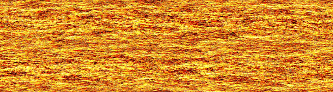
Figure 1: (Colour online) Visualizations of the instantaneous streamwise velocity in an $x$-$z$ plane at $y^{+}\approx 5$ on the stable channel side. Dark colours signify high velocities. $Re=31\,600$ and (a) $Ro=0$, (b) $Ro=0.45$, (c) $Ro=0.9$, (d) $Ro=1.2$. (e) $Re=20\,000$ and $Ro=0.45$.

Structures with a width of $O(h)$ are vaguely visible at $Ro=0$ (figure 1.a) indicating near-wall turbulence modulation by large-scale outer structures (Mathis et al. 2009). In rotating channel flow, turbulence becomes progressively weaker on the stable side with increasing rotation speeds. At low rotation rates, the flow is fully turbulent on the stable side, but at $Ro=0.45$ it is not fully turbulent anymore and regions with small-scale turbulence as well as regions where turbulence is mostly absent can be seen in figure 1.(b). The regions with small-scale turbulence have a weakly visible oblique band-like structure with an angle of about $30^{o}$ degree to the flow direction. Similar oblique patterns have been observed in e.g. transitional plane Couette flow (Barkley & Tuckerman 2007, Duguet et al. 2010) as well as in other flows with some stabilizing force like stratified open channel flow, MHD channel flow and rotating Couette flows (Brethouwer et al. 2012) and stratified Ekman layers (Deusebio et al. 2014). In rotating channel flow the turbulent-laminar patterns only exist on the stable side since the other side is fully turbulent. The turbulent-laminar patterns are not transitional but persists in time, like in the aforementioned studies.

When $Ro$ is raised to 0.9 the turbulent fraction becomes smaller and the turbulent regions appear as spots and bounded band-like oblique structures (figure 1.c) while at $Ro=1.2$ and higher no small-scale turbulence is present and only weak larger scale fluctuations are seen on the stable channel side (figure 1.d). In the latter case, a continuous cycle of strong turbulent bursts with a long period of $O(1000h/U_{b})$ on the stable side occurs caused by a linear TS wave instability (Brethouwer 2016) and a vague imprint of the TS wave is visible in figure 1. At other times the TS wave is often more prominent.

At a lower $Re=20\,000$ the flow is fully turbulent on the stable channel side at $Ro=0.15$ (shown later), whereas at $Ro=0.45$ one distinct oblique turbulent and laminar banded pattern can be observed (figure 1.e). At the same $Ro$ but a higher $Re=31\,600$ in a DNS with a larger domain turbulent-laminar patterns are more numerous but less explicit (figure 1.b). Although the angle of the oblique pattern in figure figure 1.e is determined by the periodic boundary conditions and the domain size, it is similar as the angle of the patterns seen in figure 1.b and c and the oblique patterns in other flow cases (Duguet et al. 2010, Brethouwer et al. 2012). Duguet & Schlatter (2013) argue that the obliqueness of the patterns is caused by a large-scale flow with a non-zero spanwise velocity. In previous DNSs of rotating channel flow discussed in the Introduction such patterns have not been observed, which is likely owing to the use of fairly limited computational domains.

However, Johnston et al. (1972) observed in a certain $Re$-$Ro$ range laminar flows interluded with turbulent spots on the stable channel side in their experiments confirming that such transitional flows are found at lower $Ro$ and $Re$. Dai et al. (2016) observed in DNS at $Re=7000$ and $Ro=0.3$ quasi-periodic behaviour of the wall shear stress and turbulence intensity on the stable side because the flow continuously alternated between laminar-like and intermittent with large-scale streamwise bands with either turbulent or laminar features. They attributed this quasi-periodic behaviour to the dynamics of the streamwise roll cells in their DNS. Streamwise turbulent-laminar bands, as observed by Dai et al. (2016), are not seen in the present DNSs which may be related to the size of the computational domain. On the other hand, strong quasi-periodic variations of the wall shear stress and turbulence intensity are observed in some of the present DNSs, but these were caused by a linear instability of a TS-like wave, as explained in Brethouwer (2016). This quasi-periodic behaviour is not observed in all but one DNS without this linear instability. The exception is the DNS at $Re=10\,000$ and $Ro=0.45$ where large variations of about $30\%$ are seen in the wall shear stress on the stable channel side. Visualizations (not shown here) reveal that these variations are related to quasi-periodically growing and decaying turbulent spots on this side. When the wall shear stress reaches a minimum the spots almost disappear. Large cyclic variations in the wall shear stress have also been observed in DNSs of transitional strongly stratified channel and plane Couette flows (Garcia-Villalba & del Álamo 2011, Deusebio et al. 2015), but these variations disappeared when the computational domain was enlarged, indicating that this behaviour is strongly affected by the size of domain. DNSs of spanwise rotating channel flow by Hsieh & Biringen (2016) confirm that the intermittency on the stable channel side can be strongly influenced by the computational domain size when the flow is transitional there.

Continuing with the present cases, if $Ro\geq 0.9$ and $Re=20\,000$ or lower, no turbulent spots or band-like structures are seen like in figure 1.c, illustrating that $Re$ effects can be appreciable, as discussed in more detail later. Only weak larger-scale fluctuations are observed on the stable side at high $Ro$, as illustrated in figure 1.d. However, in a number of cases the calm periods on the stable side are interrupted by violent bursts of turbulence triggered by a linear instability, as explained before.

Figure 2 shows at three different $Ro$ $\lambda_{2}$ isocontours (Jeong & Hussain 1995) coloured with the streamwise velocity to identify vortices. The strongly turbulent unstable side of the channel with intense vortices obviously shrinks with $Ro$. Between the unstable side with strong turbulence and clearly identifiable vortices and stable side with weak turbulence a seemingly sharp and flat border exists (figure 2.a-c), as was noted by Johnston et al. (1972), although when $Ro=0.9$ some areas with vortices corresponding to the patterns in figure 1.c can still be seen on the stable side.

Figure 2: (Colour online) Iso-contours of (a) $\lambda_{2}=-9$ at $Re=31\,600$ and $Ro=0.9$, (b) $\lambda_{2}=-2.25$ at $Re=31\,600$ and $Ro=1.2$, (c) $\lambda_{2}=-0.45$ at $Re=30\,000$ and $Ro=2.1$ (side views, stable channel side is at the top) and close up at iso-contours of (d) $\lambda_{2}=-5.6$ at $Re=31\,600$ and $Ro=0.9$, (e) $\lambda_{2}=-2.25$ at $Re=31\,600$ and $Ro=1.2$. The isosurfaces are coloured with streamwise velocity. The velocity increases from blue to red.

Rotation promotes the formation of streamwise vortices on the unstable side (Dai et al. 2016), especially in the region where the absolute mean vorticity is about zero (Lamballais et al. 1996). Indeed, close ups of the vortices on the border between the unstable and stable channel side at $Ro=0.9$ and 1.2 in figure 2.d and e reveal elongated streamwise vortices and, remarkably, packages of hairpin vortices which are detached from the wall. The red colour signifies that hairpin vortices are mostly found near the streamwise velocity maximum on the border between the unstable and stable channel side. At higher $Ro$ vortices including the head of the hairpin vortices become more and more aligned with the streamwise direction and hairpin vortices, as discussed by Adrian (2007), become less explicitly visible (not shown here). Yang & Wu (2016) argued that the Coriolis force reduces the inclination angle of the vortices and favours their streamwise elongation on the unstable side whereas on the stable channel side this force impedes this streamwise elongation. Lamballais et al. (1996) observed that vortices become aligned with the flow direction with $Ro$ and remarked that especially in the region where the absolute mean vorticity is about zero streamwise vortex stretching is promoted. These findings are broadly consistent with the present visualizations.

Large, steady streamwise roll cells induced by the Coriolis force have been observed on the unstable side in several experimental and numerical studies of rotating channel flow (Dai et al. 2016). Steady means here that they have a relatively long life time, although in the experiments of Johnston et al. (1972) the roll cells changed in time whereas in a DNS by Kristoffersen & Andersson (1993) they were more coherent and stationary at $Ro=0.15$ and spanned the whole channel.

Visualizations of the instantaneous wall-normal velocity field in the present DNSs are shown in figure 3. Narrow elongated streaks with positive wall-normal velocity away from the wall in a wall parallel $x$-$z$ plane on the unstable side (figure 3.a) and regions with alternating positive and negative wall-normal velocity in a cross stream $y$-$z$ plane at $Ro=0.15$ and $Re=20\,000$ (figure 3.d) indicate the presence of large streamwise roll cells on the unstable side that extend up to the border between the unstable and the stable side. The structures are long but not as coherent as in the DNS by Kristoffersen & Andersson (1993) since they appear to break up or split at some places. Possible reasons for the lesser coherency can be the higher $Re$ and the larger computational domain in the present study which puts less constrains on the dynamics of the structures through the periodic boundary conditions.

The clustering of intense vortices in streamwise near-wall streaks seen in figure 3.g show that the roll cells modulate the near-wall dynamics on the unstable side. Dai et al. (2016) observed in their DNSs of spanwise rotating channel flow that turbulence and vortices on the unstable side are stronger in the regions where the fluid is pumped away from the wall by the counter-rotating roll cells and the local mean wall shear stress has a minimum, but this augmentation was weaker at a higher $Re$. The higher vorticity was found to be caused by the Coriolis term and strong vortex stretching. This apparently contrasts the effect of large-scale motions in non-rotating wall flows. Experiments by Talluru et al. (2014) suggest the presence of large-scale counter-rotating vortices in turbulent boundary layer flow. They show that turbulence is weaker in the near-wall regions where the fluid is pumped away from the wall by these vortices and the local wall shear stress has a minimum and stronger where the large-scale motions induce a high wall shear stress, in agreement with Agostini & Leschziner (2016). The different effect of large-scale motions in non-rotating vs. rotating wall flows is presumably a result of the Coriolis term which affects both the Reynolds stresses and vorticity. Roll cells in rotating flows are likely also more coherent and steady and induce stronger wall-normal velocities.

Figure 3: (Colour online) Visualizations of the instantaneous wall-normal velocity in an $x$-$z$ plane (a) at $y=-0.5$ and $Re=20\,000$, $Ro=0.15$, (b) at $y=-0.5$ and $Re=31\,600$, $Ro=0.45$, (c) at $y=-0.75$ and $Re=31\,600$, $Ro=0.9$ and in a $y$-$z$ plane at (d) $Re=20\,000$, $Ro=0.15$, (e) $Re=31\,600$, $Ro=0.45$, (f) $Re=31\,600$, $Ro=0.9$. Dark colours signify positive velocities. (g) Isocontours of $\lambda_{2}=-36$ at $Re=20\,000$ and $Ro=0.15$ near the wall on the unstable side. The flow is from bottom left to upper right corner.

Streaks with positive wall-normal velocity (figure 3.b) and large-scale regions with positive and negative wall-normal velocity (figure 3.e) at $Ro=0.45$ and $Re=31\,600$ indicate roll cells, but they seem to be smaller and less coherent than at $Ro=0.15$. Streaky structures with a positive wall-normal velocity are seen too in figure 3.c in the DNS at $Ro=0.9$ but it is not clear if these upward and downward motions seen in figure 3.f can be interpreted as signs of roll cells. The spacing and form of the streaks indicate that the roll cells, if they exist, are smaller and less coherent than at lower $Ro$. Roll cells became smaller too in the DNS of rotating channel flow at $Re=2800$ by Dai et al. (2016) when $Ro$ was raised from 0.1 to 0.5. Signs of roll cells are visible in the DNSs at $Ro=0.45$ and 0.9 but lower $Re$ (not shown here). When $Ro=1.2$ or higher no visible signs of roll cells are found at $Re=20\,000$ and $31\,600$. However, at $Re=5000$ visualizations hint at the existence of roll cells and Grundestam et al. (2008) observed them at $Ro=1.27$ and $Re_{\tau}=180$. These observations suggest that at lower $Re$ roll cells exist up to higher $Ro$. A more quantitative study of the structures in rotating channel flow is presented in Section VII.

At higher $Ro$ the unstable turbulent side becomes smaller and smaller and the flow tends to fully laminarize if $Ro$ approaches $Ro_{c}$ (Wallin et al. 2013). Yet, even if $Ro\rightarrow Ro_{c}$, streamwise and oblique modes are still unstable as a result of rotation according to linear stability theory (Brethouwer 2016) and some of the largest linearly unstable modes become noticeable in the DNSs when turbulence gets weak on the unstable channel side. Figure 4 shows the resulting typical oblique waves on the unstable side in a DNS at $Re=30\,000$ and $Ro=2.7$, close to $Ro_{c}=2.87$ for this $Re$.

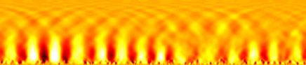
Figure 4: (Colour online) Visualization of the instantaneous wall-normal velocity for $Re=30\,000$ and $Ro=2.7$ in a (a) $y$-$z$ plane and in an (b) $x$-$z$ plane at $y=-0.8$. Colour scale ranges from $v=-0.021$ to 0.021 in b.

The waves are quite weak, i.e., the wall-normal velocity is about 2 to 3% of $U_{b}$ in this case.

IV Flow statistics

In this section, one-point statistics of the flow are presented and the effects of rotation are discussed. As mentioned before, linearly unstable TS waves cause strong recurring bursts of turbulence on a long time scale in some DNSs. The instabilities and bursts are the topic of another study (Brethouwer 2016) and therefore not discussed in detail here. However, it should be noted that they significantly affect flow structures and turbulence, especially around the bursting moment and on the stable side where the bursts are most intense. Time series of, for instance, the volume-averaged turbulent kinetic energy $K_{m}$ show distinct sharp peaks as a result of the bursts while in the calm periods between the bursts the same quantity only shows small to moderate variations, see e.g. figure 3.(b) in Brethouwer et al. (2014). I have excluded the burst periods when computing the statistics by excluding the periods with distinct peaks in $K_{m}$ caused by the linear instability. The statistics are thus based on the long relatively calm periods of $O(100h/U_{b})$ between the bursts when $K_{m}$ only shows small to moderate variations and the turbulence does not appear to be strongly influenced by the instability. The reason for excluding these bursts periods from the statistics is that the bursts are not the subject of this study and that the bursts would obscure the direct effect of rotation on the turbulence. Besides, the bursts occur on a very long time scale of $O(1000h/U_{b})$, which makes it practically impossible to obtain reasonable converged statistics if they are included, and they cannot be predicted by Reynolds stress and two-equation turbulence models. Brethouwer (2016) lists all the cases when bursts happen. At $Re=30\,000$ to $31\,600$ linear instabilities and bursts develop when $Ro\geq 1.2$. In the next parts, $U$ is the mean streamwise velocity and $u$, $v$, $w$ are the streamwise, wall-normal and spanwise velocity fluctuation, respectively. An overline implies temporal and spatial averaging in the homogeneous directions.

Figure 5 shows mean streamwise velocity profiles scaled by $U_{b}$ at the highest $Re$ considered for $Ro$ up to 2.7. As in previous studies of turbulent channel flow subject to spanwise rotation (e.g. Kristoffersen & Andersson 1993, Grundestam et al. 2008, Xia et al. 2016), the mean velocity profile becomes asymmetric and develops an extended linear region where the slope $\mbox{d}U/\mbox{d}y\simeq 2\Omega$, i.e. $S\simeq-1$, implying an absolute mean vorticity close to zero.

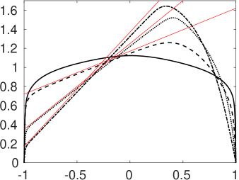
Figure 5: (Colour online) Mean velocity profiles scaled by $U_{b}$. (a) $Re=31\,600$. $~{}^{\line(1,0){20.0}}$, $Ro=0$; $---$, $Ro=0.45$; $\cdot\cdot\cdot$, $Ro=0.9$; $-\cdot-\cdot-$, $Ro=1.2$. (b) $Re=30\,000$. $~{}^{\line(1,0){20.0}}$, $Ro=1.5$; $---$, $Ro=2.1$; $\cdot\cdot\cdot$, $Ro=2.4$; $-\cdot-\cdot-$, $Ro=2.7$. Slopes with $S=-1$ are shown by straight red lines.

If $Ro\leq 1.5$ the velocity on the unstable side goes down while on the stable side it goes up since the turbulence becomes stronger and weaker on the unstable and stable side, respectively, as will be shown later. At higher $Ro$, the profile becomes more and more parabolic-like and beyond $Ro=2.4$ the linear slope region disappears and the velocity profile approaches a laminar Poiseuille profile, as in the DNSs by Grundestam et al. (2008) and Xia et al. (2016).

Profiles of the root-mean-square (rms) of the streamwise, wall-normal and spanwise velocity fluctuations, $u^{+}$, $v^{+}$ and $w^{+}$, respectively, and the Reynolds shear stress $\overline{uv}^{+}$ normalized by $u_{\tau}[u^{2}_{\tau u}/2+u^{2}_{\tau s}/2]^{1/2}$ for $Ro$ up to 2.1 are shown in figure 6. The results are for the highest $Re$ considered here, $31\,600$ and $30\,000$.

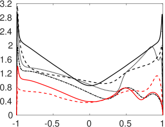
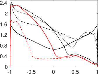
Figure 6: (Colour online) Rms profiles of (a) streamwise, (b) wall-normal (c) spanwise velocity fluctuations and (d) $\overline{uv}$ profiles in wall units. $Re=31\,600$ and ($~{}^{\line(1,0){20.0}}$) $Ro=0$, ($---$) $Ro=0.45$, ($\cdot\cdot\cdot$) $Ro=0.9$, ($-\cdot-\cdot-$) $Ro=1.2$. $Re=30\,000$ and (${\color[rgb]{1,0,0}~{}^{\line(1,0){20.0}}}$) $Ro=1.5$, (${\color[rgb]{1,0,0}---}$) $Ro=2.1$.

Note that for $Ro\geq 1.2$ the flow is subject to a TS-wave instability resulting in intense bursts of turbulence at this $Re$ (Brethouwer 2016), but these periods with turbulent bursts are excluded as much as possible when computing the statistics as mentioned before. The statistics are thus based on the long calm periods between the bursts.

Figure 6 shows that rotation causes a reduction of the turbulence intensity on the stable side, as expected (Johnston et al. 1972). Especially for the wall-normal component (figure 6.b) this reduction is apparent while for the other two velocity components it becomes most notable for $Ro\geq 1.2$. The turbulence on the unstable channel side displays a more complex behaviour. The peak of $u^{+}$ first raises with $Ro$ but then declines if $Ro>0.45$ whereas $w^{+}$ and especially $v^{+}$ strongly grow with $Ro$ and only start to notably decline when $Ro>1.5$. At higher $Ro$ turbulence is progressively suppressed (not shown here) and the flow approaches more and more a laminar Poiseuille flow, as observed for the mean flow. Rotation has thus not only a marked influence on the turbulence intensity but also on its anisotropy, as in rotating homogeneous shear flows (Brethouwer 2005). The observed trends are in qualitative agreement with DNSs of rotating channel flow at lower $Re$ (Grundestam et al. 2008). The maximum of $v^{+}$ is near the wall at $Ro=0$ but remarkably far from the wall on the unstable side at $Ro=0.45$, which may be due to the presence of roll cells, while at higher $Ro$ it approaches the wall again.

From the mean momentum balance for rotating channel flow follows

$$-\overline{uv}+\nu\frac{\mbox{d}U}{\mbox{d}y}=u^{2}_{\tau u}-u^{2}_{\tau}(y+1),$$ (3)

where the velocities are dimensional. The sum of the viscous and turbulent shear stresses is thus linear in $y$ but is shifted owing to the difference in the wall shear stresses on the unstable and stable channel sides in the rotating flow cases. These stresses are naturally higher on the unstable side owing to the more intense turbulence. When viscous stresses are negligible the $\overline{uv}^{+}$ profile is also linear in $y$ according to equation (3). From this equation follows that in the part of the channel where $\nu\mbox{d}U/\mbox{d}y\simeq 2\nu\Omega=U^{2}_{b}Ro/Re$ the turbulent shear stress approximates

$$\overline{uv}\simeq u^{2}_{\tau}(y+1)-u^{2}_{\tau u}+U^{2}_{b}\frac{Ro}{Re}.$$ (4)

This shows that the $\overline{uv}^{+}$ profile is linear in $y$ and has a unit slope even if viscous stresses are not negligible (Xia et al. 2016). Figure 6.(d) confirms that on the unstable side the $\overline{uv}^{+}$ profiles have a unit slope. The turbulent momentum transfer shifts progressively towards the unstable side with $Ro$ and for $Ro\geq 1.2$ it is in fact negligible on the stable side where viscous stresses dominate. On the unstable side the magnitude of $\overline{uv}^{+}$ starts to decline when $Ro>0.9$ and is small for $Ro\geq 2.1$. Viscous shear stresses are significant on the strongly turbulent unstable channel side at higher $Ro$ because of the steep mean velocity gradient. If the total shear stress is estimated as $u^{2}_{\tau}$, it follows that on the unstable side where $\mbox{d}U/\mbox{d}y\simeq 2\Omega$ the ratio between viscous and total stresses is approximately $Ro\,Re/Re^{2}_{\tau}$. From that follows that the viscous contribution grows with $Ro$ and is about 12% and 26% at $Re=31\,600$ and $Ro=1.2$ and 1.5, respectively, and even higher at the same $Ro$ but lower $Re$. Once $Ro\gtrsim 2.0$ viscous stresses dominate also on the unstable side.

To investigate in more detail the turbulence near the wall on the unstable channel side, I present in figure 7 rms-profiles of the streamwise, wall-normal and spanwise velocity fluctuations, $u^{*}$, $v^{*}$, $w^{*}$ respectively, in viscous wall units of the unstable side using a logscale for $y^{*}$.

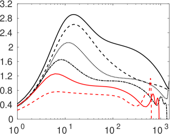
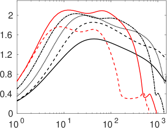
Figure 7: (Colour online) Rms profiles of (a) streamwise, (b) wall-normal and (c) spanwise velocity fluctuations in wall units of the unstable side. $Re=31\,600$ and ($~{}^{\line(1,0){20.0}}$) $Ro=0$, ($---$) $Ro=0.45$, ($\cdot\cdot\cdot$) $Ro=0.9$, ($-\cdot-\cdot-$) $Ro=1.2$. $Re=30\,000$ and (${\color[rgb]{1,0,0}~{}^{\line(1,0){20.0}}}$) $Ro=1.5$, (${\color[rgb]{1,0,0}---}$) $Ro=2.1$.

Velocity fluctuations are thus scaled by $u_{\tau u}$ and $y^{*}=(y+1)u_{\tau u}/\nu$ since $u_{\tau u}$ appears to be the most relevant quantity very close to the wall. Note that $u_{\tau u}$ can deviate quite significantly from $u_{\tau}$, see table 1. The peak of $u^{*}$ on the unstable side declines and moves towards smaller $y^{*}$ with $Ro$ whereas the peaks of $v^{*}$ and $w^{*}$ grow with $Ro$ until $Ro=1.5$ and then decline. This reduction and growth respectively are caused by an energy redistribution from streamwise to wall-normal fluctuations by the Coriolis term and pressure-strain correlations in the Reynolds stress equations, as will be shown later. The peak of $w^{*}$ moves towards the wall with $Ro$ whereas that of $v^{*}$ is found far away from the wall at $Ro=0.45$ and comes closer to the wall with increasing $Ro$. The profile of $w^{*}$ has two peaks for $Ro\geq 1.2$ which is accompanied by a double peak in the spectra as shown later.

The skewness of the streamwise velocity $S(u)$ and wall-normal velocity fluctuations $S(v)$ are presented in figure 8. Profiles of $S(u)$ and $S(v)$ at lower $Re$ are presented by Hsieh & Biringen (2016). $S(u)$ is typically negative away from the wall in non-rotating channel flow owing to ejections of low speed fluid (Kim et al. 1987). In rotating channel flow $S(u)$ becomes considerably more negative near the wall at $Ro=0.45$ and 0.9 on the unstable side, except very near the wall. This could be caused by a reduction of sweeping events of high-speed flow towards the wall as a consequence of rotation (Kristoffersen & Andersson 1993). On the other hand, the analysis by Dai et al. (2016) indicates that under the influence of rotation the streaks become stronger on the unstable side, at least up to moderate $Ro$, which implies more or intenser ejections. The roll cells, observed before, could also play a role. If $Ro>0.9$, $S(u)$ becomes less negative near the wall, which can be related to the weaker streaks and related ejections at high $Ro$, as suggested by Lamballais et al. (1998). Further away from the wall $S(u)$ attains small values in the rotating cases compared to the non-rotating case indicating that sweeping and ejection events are significantly altered by rotation.

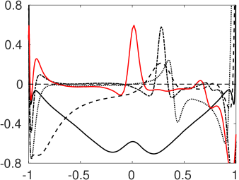
Figure 8: (Colour online) Skewness of (a) $u$ and (b) $v$. $Re=31\,600$ and ($~{}^{\line(1,0){20.0}}$) $Ro=0$, ($---$) $Ro=0.45$, ($\cdot\cdot\cdot$) $Ro=0.9$, ($-\cdot-\cdot-$) $Ro=1.2$. $Re=30\,000$ and (${\color[rgb]{1,0,0}~{}^{\line(1,0){20.0}}}$) $Ro=1.5$.

$S(v)$ has a large positive value near the wall on the unstable side at $Ro=0.45$ compared to $Ro=0$ which is likely caused by roll cells that induce high-speed wall-normal velocity away from the wall. Similar behaviour of $S(v)$ was observed in the experiments by Nakabayashi & Kitoh (2015). Large positive values of $S(v)$, indicating events with large positive wall-normal velocities, are also found in all rotating cases on the unstable side quite close to the position where the slope of $U$ begins to deviate from $2\Omega$. At $Ro=1.2$ and 1.5, $S(u)$ has large values at slightly larger $y$ near the position where $U$ has its maximum value. The reason for the large values of $S(u)$ and $S(v)$ around these positions is not fully clear, but visualizations suggest that large values of $v$ are found near the streamwise vortices visualized in figure 2. The large $S(u)$ could be related to the hairpin vortices seen in figure 2 since positive values of $u$ are found above the head of such hairpin vortices (Christensen & Adrian 2001, Adrian 2007).

The flatness of the wall-normal velocity $F(v)$ attains extreme values in non-rotating channel flow very near the wall as a result of intense near-wall vortices (Lenaers et al. 2012). The present DNSs show that with faster rotation $F(v)$ on the unstable channel side monotonically decays with $Ro$ suggesting that intense near-wall vortices are suppressed.

V Influence of the Reynolds number

In this section, the influence of the Reynolds number on rotating channel flow at a fixed $Ro$ is examined and shown to be significant. In a later section, this influence on the flow structures found on the unstable channel side is investigated.

Figure 9 shows profiles of the mean velocity $U/U_{b}$ and fluctuations $v^{+}$ at $Ro=0.15$, 0.45 and 0.9 for three to four $Re$.

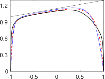
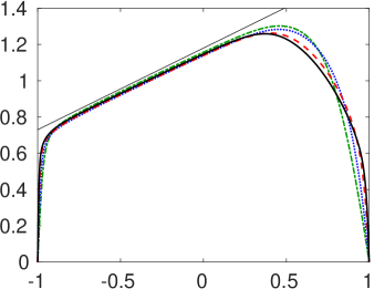
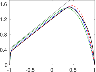
Figure 9: (Colour online) (a) Mean velocity profiles scaled by $U_{b}$ and (b) rms of $v$ in wall units at $Ro=0.15$ and $~{}^{\line(1,0){20.0}}$, $Re=20\,000$; ${\color[rgb]{1,0,0}---}$, $Re=5000$; ${\color[rgb]{0,0,1}\cdot\cdot\cdot}$, $Re=3000$. (c) Mean velocity profiles scaled by $U_{b}$ and (d) rms of $v$ in wall units at $Ro=0.45$ and $~{}^{\line(1,0){20.0}}$, $Re=31\,600$; ${\color[rgb]{1,0,0}---}$, $Re=20\,000$; ${\color[rgb]{0,0,1}\cdot\cdot\cdot}$, $Re=10\,000$; ${\color[rgb]{0,1,0}-\cdot-\cdot-}$, $Re=5000$. (e) and (f) are the same as (c) and (d), respectively, but for $Ro=0.9$. The straight black line has a slope $S=-1$.

In all cases a region with a linear mean velocity profile where $S\simeq-1$ can be readily recognised demonstrating once more that the appearance of a region with a zero absolute mean vorticity is a fundamental feature of rotating channel flow. Its extent and the closeness of $\mbox{d}U/\mbox{d}y$ to $2\Omega$ do not show much variation with $Re$ and the same applies to the maximum value of $v^{+}$ on the unstable channel side. On the other hand, $Re$ has an obvious influence on the mean velocity profile as well as $v^{+}$ on the stable channel side where at higher $Re$ $v^{+}$ is considerably larger.

This Reynolds number effect is also observed in visualizations of the instantaneous streamwise velocity in a plane parallel and close to the wall on the stable channel side.

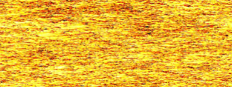
Figure 10: (Colour online) Visualizations of the instantaneous streamwise velocity in an $x$-$z$ plane at $y^{+}\approx 5$ on the stable channel side. Dark colours signify high velocities. (a) $Ro=0.15$ and $Re=20\,000$, (b) $Ro=0.15$ and $Re=3000$ and (c) $Ro=0.45$ and $Re=5000$.

At $Ro=0.15$ and $Re=20\,000$ the flow is fully turbulent on the stable channel side (figure 10.a) whereas at a lower $Re=3000$ the flow is largely laminar and contains only some turbulent spots (figure 10.b) resulting in much lower turbulence levels on the stable channel side (figure 9.b). At $Ro=0.45$ and $Re=31\,600$ a large fraction of the flow on the stable side is turbulent and turbulent-laminar patterns develop, as shown before in figure 1.(b), whereas at the same $Ro$ but lower $Re=5000$ the flow is predominantly laminar and only one turbulent spot can be observed (figure 9.c). At a lower $Re=3000$ the spot is even smaller. Also at $Ro=0.9$ and $Re=31\,600$ regions with small-scale turbulence can be observed (figure 1.c), but these regions with small-scale turbulence are completely absent at lower $Re$ (not shown here). $Re$ has thus a marked influence on the flow, especially on the stable channel side, with a growing turbulent fraction and stronger turbulence at fixed $Ro$ when $Re$ gets higher. In the present study, oblique turbulent-laminar patterns have only been observed at higher $Re$. A speculation is that they also exist at low $Re$ although at a lower $Ro$ when the stabilizing Coriolis force is less strong. But at a lower $Re$ they can have a longer wave length, as indicated by Brethouwer et al. (2012), implying that very large computational domains are required to resolve them.

Profiles of the rms of the velocity fluctuations in terms of wall units of the unstable side, i.e., velocity fluctuations scaled by $u_{\tau u}$ and $y^{*}=yu_{\tau u}/\nu$, for different $Ro$ and $Re$ are not presented here. However, the peak of the streamwise and spanwise fluctuations in general increases with $Re$ at fixed $Ro$ whereas the maximum of the wall-normal fluctuations is quite independent of $Re$ but moves towards larger $y^{*}$ with $Re$.

The volume-averaged turbulent kinetic energy $K_{m}$ scaled by $U^{2}_{b}$, mean wall shear stresses $\tau^{u}_{w}$ and $\tau^{s}_{w}$ on the unstable and stable channel sides respectively, and skin friction coefficient $C_{f}=\tau_{w}/(\frac{1}{2}\rho U^{2}_{b})$ with $\tau_{w}=\frac{1}{2}(\tau^{u}_{w}+\tau^{s}_{w})$ are shown in figure 11 at different $Ro$ and $Re$.

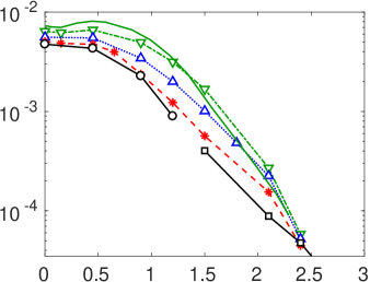
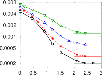
Figure 11: (Colour online) (a) $K_{m}/(U^{2}_{b})$, (b) $\tau^{u}_{w}/\tau_{w}$ (upper curves) and $\tau^{s}_{w}/\tau_{w}$, (c) $C_{f}$. $\circ^{\line(1,0){20.0}}\circ$, $Re=31\,600$; $\boxempty^{\line(1,0){20.0}}\boxempty$, $Re=30\,000$; ${\color[rgb]{1,0,0}\ast---\ast}$, $Re=20\,000$; ${\color[rgb]{0,0,1}\Delta\cdot\cdot\cdot\Delta}$, $Re=10\,000$; ${\color[rgb]{0,1,0}\nabla-\cdot-\cdot-\nabla}$, $Re=5000$; ${\color[rgb]{0,1,0}~{}^{\line(1,0){20.0}}}$, $Re_{\tau}=180$ (Xia et al. 2016). The horizontal line in (c) represent $C_{f}$ for a laminar Poiseuille flow.

Figure 11.(a) shows that overall the turbulence intensity decays with $Ro$ at fixed $Re$ and becomes very weak at high $Ro$ with similar trends for all $Re$. The data of Xia et al. (2016) are also included in the figure and show first a 15% growth in $K_{m}/U^{2}_{b}$ until $Ro=0.44$ and then a quite similar decay as in the other cases, but note that in their DNS series $Re_{\tau}=180$ and constant and therefore $Re$ varies. The difference in $\tau_{w}$ on the stable and unstable side first grows substantially with $Ro$ until its maximum found around $Ro=0.9$, with the highest $\tau_{w}$ naturally occurring on the unstable side, but then diminishes and disappears at high $Ro$ when the flow becomes laminar (figure 11.b). Again, the trends are similar at different $Re$ but the maximum difference appears at lower $Ro$ when $Re$ is lower and is smaller at the highest $Re$, possibly because the flow relaminarizes less fast on the stable side at higher $Re$, as discussed before. The skin friction $C_{f}$ decays monotonically with $Ro$, like $K_{m}$, and nearly equals the value for laminar Poiseuille flow for $Ro\geq 2.4$ at all $Re$ (figure 11.c).

VI Balances

In this section, the balance terms in the transport equations of the turbulent kinetic energy and Reynolds stresses are studied. Grundestam et al. (2008) have also presented budgets for rotating channel flow, although only for one high $Ro=1.5$ when the turbulence is very weak, while Xia et al. (2016) have only presented production terms. The present study contributes with a study of several budgets terms at a significantly higher $Re$ covering a wide $Ro$ range.

From equation (4) follows that the production of turbulent kinetic energy in the part of the channel where $\mbox{d}U/\mbox{d}y\simeq 2\Omega$ is approximately (see also Xia et al. 2016)

$$P_{K}=-\overline{uv}\frac{\mbox{d}U}{\mbox{d}y}\simeq-2\overline{uv}\Omega=-\overline{uv}\frac{U_{b}}{h}Ro\simeq\left[u^{2}_{\tau u}-u^{2}_{\tau}(y+1)-U^{2}_{b}\frac{Ro}{Re}\right]\frac{U_{b}}{h}Ro$$ (5)

Consequently,

$$\frac{hP_{K}}{u^{2}_{\tau}U_{b}Ro}\simeq-(y+1)+\left(\frac{u_{\tau u}}{u_{\tau}}\right)^{2}-\left(\frac{U_{b}}{u_{\tau}}\right)^{2}\frac{Ro}{Re}.$$ (6)

Thus, the profile of $P_{K}$ scaled with $u^{2}_{\tau}U_{b}Ro/h=(u^{4}_{\tau}/\nu)(Ro_{\tau}/Re_{\tau})$, where $u^{4}_{\tau}/\nu$ is the usual viscous wall unit scaling, is expected to be approximately linear in $y$ with a slope $-1$ in the part of the channel where $\mbox{d}U/\mbox{d}y\simeq 2\Omega$.

Figure 12.(a) shows $P_{K}$ scaled by $u^{2}_{\tau}U_{b}Ro/h$ for $Ro$ up to 2.1.

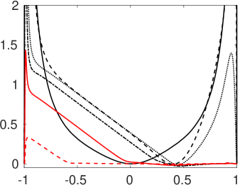
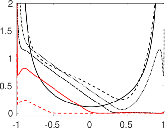
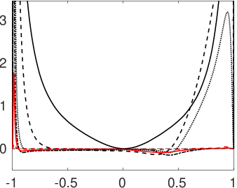
Figure 12: (Colour online) (a) $P_{K}$ scaled by $u^{2}_{\tau}U_{b}Ro/h$ and (b) $P_{K}$ scaled by $u^{4}_{\tau u}/\nu$. (c) $\varepsilon$ and (d) $P_{uv}$ and (e) $P^{tot}_{uu}=P_{uu}+C_{uu}$ and (f) $P^{tot}_{uv}=P_{uv}+C_{uv}$ scaled by $u^{2}_{\tau}U_{b}Ro/h$. $Re=31\,600$ and ($~{}^{\line(1,0){20.0}}$) $Ro=0$, ($---$) $Ro=0.45$, ($\cdot\cdot\cdot$) $Ro=0.9$, ($-\cdot-\cdot-$) $Ro=1.2$. $Re=30\,000$ and (${\color[rgb]{1,0,0}~{}^{\line(1,0){20.0}}}$) $Ro=1.5$, (${\color[rgb]{1,0,0}---}$) $Ro=2.1$.

The DNS results for $Ro=0$ are included and scaled by $0.45u^{2}_{\tau}U_{b}/h$, i.e., the same scaling as used for the $Ro=0.45$ case. The profiles of $P_{K}$ in the rotating cases show as expected a significant linear part with a $-1$ slope. In this part, the scaled $P_{K}$ follows closely the prediction given by the right-hand-side of equation (6). Similar linear profiles of $P_{K}$ were observed in DNSs of rotating channel flow at $Re_{\tau}=180$ by Xia et al. (2016). Near the maximum of $U$ slight negative values of $P_{K}$ are observed at some $Ro$, as in a DNS by Grundestam et al. (2008), which implies that some energy is transferred from turbulence to the mean flow in this region. The maximum value of $P_{K}$ near the wall on the unstable side scales instead with viscous walls units since the peak of $P_{K}$ lies between 0.244 and 0.248 for $Ro\leq 1.5$ when scaled by $u^{4}_{\tau u}/\nu$ (figure 12.b).

In shear flows, the dissipation rate of turbulent kinetic energy, $\varepsilon$, is often approximately equal to the production of turbulent kinetic energy, $P_{K}$, which suggests that $\varepsilon$, like $P_{K}$, scales with $u^{2}_{\tau}U_{b}Ro/h$. Figure 12.(c) affirms that in rotating channel flow profiles of $\varepsilon$, scaled by $u^{2}_{\tau}U_{b}Ro/h$, display a linear part. The DNS results for $Ro=0$ are again included and scaled by $0.45u^{2}_{\tau}U_{b}/h$. The slopes at $Ro=0.45$ and $Ro=2.1$ deviate from $-1$, but in the other three rotating cases it follows closely the prediction given by the right-hand-side of equation (6). For $Ro\geq 0.9$, $P_{K}$ and $\varepsilon$ are in fact strikingly similar in the outer layer on the unstable channel side, much more so than at $Ro=0$. The close balance between $P_{K}$ and $\varepsilon$ implies that the sum of turbulent, pressure and viscous diffusion in the equation for turbulent kinetic energy is small compared to $P_{K}$ and $\varepsilon$. In terms of wall units, $P_{K}$ and $\varepsilon$ are large on the unstable side away from the wall in the rotating cases compared to the $Ro=0$ case whereas on the stable side both are very small if $Ro\geq 1.2$.

The observed scaling of $P_{K}$ and $\varepsilon$ with $u^{2}_{\tau}U_{b}Ro/h$ suggests that this scaling is meaningful as well for the budget terms in the balance equation for the Reynolds stresses. This equation reads

$$\frac{\partial\overline{u_{i}u_{j}}}{\partial t}+U_{k}\frac{\partial\overline{u_{i}u_{j}}}{\partial x_{k}}=P_{ij}+\varepsilon_{ij}+C_{ij}+\Pi_{ij}+D_{ij},$$ (7)

where the terms on the right-hand-side are the production, dissipation, Coriolis, pressure-strain and diffusion term respectively (Grundestam et al. 2008). The Coriolis terms in the equation for $\overline{uu}$, $\overline{vv}$, $\overline{ww}$ and $\overline{uv}$ stresses are $C_{uu}=4\overline{uv}\Omega$, $C_{vv}=-4\overline{uv}\Omega$, $C_{ww}=0$ and $C_{uv}=2(\overline{vv}-\overline{uu})\Omega$, respectively. These terms do not perform work but transfer energy between the Reynolds stress components (Kawata & Alfredsson 2016). Note that $P_{uu}\,=\,2P_{K}$.

Figure 12.(d) shows the production of $\overline{uv}$ Reynolds stresses, $P_{uv}\,=\,-\overline{vv}\mbox{d}U/\mbox{d}y$, scaled by $u^{2}_{\tau}U_{b}Ro/h$. Also in this figure and figure 13, data for $Ro=0$ are included using the scaling $0.45u^{2}_{\tau}U_{b}/h$ to make a comparison with data of rotating channel flow possible. The profiles of $P_{uv}$ show less spreading than when using the ordinary wall unit scaling and also reveal an approximately linear slope on the unstable side if $Ro\geq 0.9$. On the stable side $P_{uv}$ is significant at $Ro=0.45$ but negligible for $Ro\geq 1.2$.

The Coriolis terms in the balance equations of the $\overline{uu}$ and $\overline{vv}$ Reynolds stresses are $C_{uu}=2\overline{uv}/u^{2}_{\tau}$ and $C_{vv}=-2\overline{uv}/u^{2}_{\tau}=-C_{uu}$ respectively, when scaled by $u^{2}_{\tau}U_{b}Ro/h$. Profiles of $\overline{uv}/u^{2}_{\tau}$ were already presented in figure 6.(d). From these profiles it follows that on the unstable side the Coriolis term transfers energy from $\overline{uu}$ to the $\overline{vv}$ component in rotating channel flow. On the stable side it is the other way around for $Ro=0.45$ and 0.9 whereas it is small in the other cases.

If $\mbox{d}U/\mbox{d}y\simeq 2\Omega$, $P_{uu}\simeq-4\overline{uv}\Omega=-C_{uu}$, which means that the Coriolis term closely balances the production term and, consequently, the dissipation term approximately balances the pressure-strain term in the equation for the $\overline{uu}$ component since the transport terms are small. This is confirmed by the DNSs but not shown here. In fact, the sum $P_{ij}+C_{ij}\equiv P^{tot}_{ij}$ may be considered as a total production term. When $\mbox{d}U/\mbox{d}y\simeq 2\Omega$, $P^{tot}_{uu}\simeq 0$, $P^{tot}_{vv}\simeq P_{uu}$ and $P^{tot}_{ww}\simeq 0$ since $P_{uu}\simeq-C_{uu}=C_{vv}$ as explained above and $P_{vv}=P_{ww}=C_{ww}=0$. Figure 12.(e) shows $P^{tot}_{uu}$ scaled by $u^{2}_{\tau}U_{b}Ro/h$ and confirms that in a large part of a rotating channel flow it is nearly zero. Thus, in a non-rotating flow, production feeds energy in the $\overline{uu}$ component and then energy is redistributed to the other components. By contrast, in rotating channel flow on the unstable side $P^{tot}_{ij}$ feeds energy mainly in the $\overline{vv}$ component and pressure-strain correlations redistribute this energy to the $\overline{uu}$ and $\overline{ww}$ components. This may explain the strong wall-normal velocity fluctuations observed in rotating channel flow on the unstable side. Very near the wall on the unstable side energy is still fed into the $\overline{uu}$ component. The same applies to the stable side for $Ro=0.45$ and 0.9 but if $Ro\geq 1.2$ the sum is nearly zero. Note that $P^{tot}_{uu}$ is slightly negative in rotating channel flow in a region around the maximum of $U$.

When scaled by $u^{2}_{\tau}U_{b}Ro/h$, $C_{uv}=(\overline{vv}-\overline{uu})/u^{2}_{\tau}$. The total production $P^{tot}_{uv}$ scaled by $u^{2}_{\tau}U_{b}Ro/h$, shown in figure 12.(f), is balanced by $\Pi_{uv}$ since the dissipation and diffusion terms are relatively small in a large part of the channel, in particular on the unstable side. On the unstable side, $P^{tot}_{uv}$ scaled is negative, but it becomes less negative for $Ro\geq 0.9$. On the stable side it is positive at $Ro=0.45$ and negative at larger $Ro$ meaning that it destroys $\overline{uv}$ correlations, leading to the low turbulent shear stresses on the stable side observed before.

Pressure-strain correlations $\Pi_{uu}$, $\Pi_{vv}$, $\Pi_{ww}$ and $\Pi_{uv}$ scaled by $u^{2}_{\tau}U_{b}Ro/h$ are presented in figure 13.

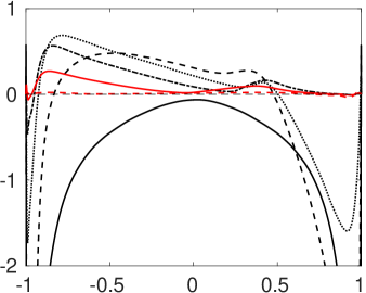
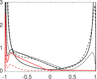
Figure 13: (Colour online) (a) $\Pi_{uu}$, (b) $\Pi_{vv}$, (c) $\Pi_{ww}$ and (d) $\Pi_{uv}$ scaled by $u^{2}_{\tau}U_{b}Ro/h$. Lines used as in figure 12.

When $Ro=0$ energy is transferred from $\overline{uu}$ to $\overline{vv}$ and $\overline{ww}$, whereas in the rotating cases energy is transferred from $\overline{vv}$ to $\overline{uu}$ and $\overline{ww}$ by pressure-strain correlations on the unstable side, except very close to the wall where $\Pi_{uu}$ is still negative. Especially at high $Ro$, $\Pi_{ww}$ is large which explains the strong spanwise fluctuations in rapidly rotating channel flows. On the stable side there is a significant energy transfer from $\overline{uu}$ to the other two components by pressure-strain correlations for $Ro\leq 0.9$. At larger $Ro$, $\Pi_{uu}$ and $\Pi_{vv}$ are small but not negligible on the stable side while $\Pi_{uv}$ is positive (figure 13.d) and approximately balanced by the Coriolis term $C_{uv}$ as discussed before. The slope of the pressure-strain profiles on the unstable side is also approximately linear for $Ro\geq 0.9$ and scales with $u^{2}_{\tau}U_{b}Ro/h$.

Turbulent velocity fluctuations are not insignificant on the stable side (figure 6), although $P_{K}$ is very small there for $Ro\geq 1.2$. Grundestam et al. (2008) have suggested that the turbulence on the stable side is forced by the turbulence on the unstable side through the pressure diffusion term of the $\overline{vv}$ component which then redistributes the energy through pressure-strain correlations. The pressure diffusion of $\overline{vv}$ has indeed a small positive value (not shown here) and figure 13.(a) and (b) show that, albeit small, $\Pi_{vv}$ is negative and $\Pi_{uu}$ positive at $Ro=1.2$ and 1.5 on the stable side. The latter is approximately balanced by a negative $P^{tot}_{uu}$.

VII Spectra and two-point correlations

In order to study the effect of rotation on turbulence structures in a quantitative way Kristoffersen & Andersson (1993), Alvelius (1999) and Grundestam et al. (2008) computed two-point correlations at $Re_{\tau}=180$ to 194. Kristoffersen & Andersson observed that the spanwise near-wall streak spacing in wall units narrows with $Ro$ whereas Alvelius observed the opposite trend. Generally, relatively short streamwise two-point correlations of streamwise fluctuations on the unstable side and relatively long ones on the other laminar-like side were observed when the channel was rotating. At low $Ro$ Kristoffersen & Andersson and Alvelius could also notice an impact of Taylor-Görtler vortices on correlations on the unstable side.

Here, I present spanwise two-point correlations of the wall-normal velocity fluctuations as well as spectra since they reveal better the impact of rotation on the different flow scales, especially the large scales which are known to become important at higher $Re$ in wall flows (Smits et al. 2011). Spectra of the streamwise velocity fluctuations are presented since these most clearly reveal the presence of large-scale motions in non-rotating wall flows as well as spectra of the spanwise and wall-normal velocity fluctuations since these may uncover the presence of roll cells. The presented co-spectra give information on the scales that contribute to the momentum transfer and production of turbulent kinetic energy. The focus is on the strongly turbulent unstable side of the channel. Spectra and two-point correlations are less instructive for the stable side when relaminarization occurs. First, I consider the trends with $Ro$ and next with $Re$.

VII.1 Spectra at $Re=20\,000$

Spanwise premultiplied energy spectra, $k_{z}\Phi_{uu}$, $k_{z}\Phi_{vv}$ and $k_{z}\Phi_{ww}$ of the streamwise, wall-normal and spanwise velocity fluctuations, respectively, and cospectra, $k_{z}\Phi_{uv}$, at $Re=20\,000$ are shown in figure 14. Streamwise premultiplied energy spectra, $k_{x}\Phi_{uu}$, $k_{x}\Phi_{vv}$ and $k_{x}\Phi_{ww}$ of the streamwise, wall-normal and spanwise velocity fluctuations, respectively, and cospectra, $k_{x}\Phi_{uv}$, at $Re=20\,000$ are shown in figure 15. Spectra are shown for $Ro=0$, 0.15, 0.45 and 0.9, and are presented as function of the wall distance $y^{*}=(y+1)u_{\tau u}/\nu$ and the spanwise and streamwise wave length $\lambda^{*}_{z}$ and $\lambda^{*}_{x}$, respectively, both scaled in term of the viscous length scale of the unstable side, $l^{*}=\nu/u_{\tau u}$. The red dashed line in each plot indicates scales with a wavelength $h$. Spectra are scaled with their maximum value, which are given in terms of $u_{\tau u}$ in table 2.

$Re$	$Ro$	$k_{z}\frac{\Phi_{uu}}{u^{2}_{\tau u}}^{\star}$	$k_{z}\frac{\Phi_{vv}}{u^{2}_{\tau u}}^{\star}$	$k_{z}\frac{\Phi_{ww}}{u^{2}_{\tau u}}^{\star}$	$k_{z}\frac{\Phi_{uv}}{u^{2}_{\tau u}}^{\star}$	$k_{x}\frac{\Phi_{uu}}{u^{2}_{\tau u}}^{\star}$	$k_{x}\frac{\Phi_{vv}}{u^{2}_{\tau u}}^{\star}$	$k_{x}\frac{\Phi_{ww}}{u^{2}_{\tau u}}^{\star}$	$k_{x}\frac{\Phi_{uv}}{u^{2}_{\tau u}}^{\star}$
$20\,000$	0	3.83	0.56	0.73	0.58	2.13	0.40	0.66	0.28
$20\,000$	0.15	3.85	0.75	1.00	0.57	2.15	0.32	0.56	0.28
$20\,000$	0.45	3.01	1.60	1.39	0.49	1.89	0.59	0.64	0.27
$20\,000$	0.9	1.67	2.13	1.86	0.46	1.24	1.04	0.95	0.29
$5000$	0		0.50	0.64			0.33	0.57
$5000$	0.45		1.61	1.32			0.61	0.61
$5000$	0.9		2.50	1.85			1.16	0.96

Table 2: Maximum values of the premultiplied one-dimensional energy spectra. Superscript $\star$ means the maximum value of the quantity. The spectra are scaled with the friction velocity of the unstable side, $u_{\tau u}$.

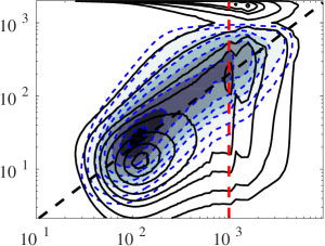
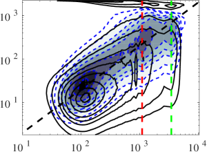
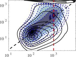
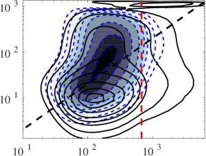
Figure 14: (Colour online) Maps of premultiplied one-dimensional energy spectra as function of spanwise wavelength $\lambda^{*}_{z}$ and distance from the wall $y^{*}$ at $Re=20\,000$ for $Ro=0$ (a, b), $Ro=0.15$ (c, d), $Ro=0.45$ (e, f) and $Ro=0.9$ (g, h). Left column shows $k_{z}\Phi_{uu}$ (black lines) and cospectra $k_{z}\Phi_{uv}$ (blue dashed lines and colours). Right column shows $k_{z}\Phi_{vv}$ (blue dashed lines and colours) and $k_{z}\Phi_{ww}$ (black lines). Contour levels from innermost to outermost are 0.94, 0.8, 0.6, 0.4, 0.28, 0.2, 0.1 and 0.05. Spectra are scaled with their maximum value. The straight black dashed line follows the relation $y=0.1\lambda_{z}$.

Roll cells produce significant wall-normal and spanwise motions in rotating channel flow, as shown by e.g. Dai et al. (2016), and that can be expected to lead to energetic large-scale modes in the spectra of the spanwise and especially the wall-normal velocity away from the wall. I therefore interpret distinctly energetic large-scale modes in the spanwise $k_{z}\Phi_{vv}$ and $k_{z}\Phi_{ww}$ spectra as well as in the streamwise $k_{x}\Phi_{vv}$ spectra as signs of roll cells. If there are $n$ pairs of counter-rotating roll cells in the computational domain, which has a spanwise size of $L_{z}=3\pi h$ in these DNSs, the spanwise spectrum $k_{z}\Phi_{vv}$ can be expected to have a peak at $\lambda_{z}=3\pi h/n$.

In non-rotating channel flow the spanwise spectra reveal, besides the streaks at $\lambda^{*}_{z}\approx 100$ indicated by the near-wall peak in $k_{z}\Phi_{uu}$, the signature of large wide structures of wavelength $\lambda_{z}\approx h$ in $k_{z}\Phi_{uu}$ and $k_{z}\Phi_{uv}$ further away from the wall, (figure 14.a), like in the DNS by Lee & Moser (2015). In the streamwise spectra $k_{x}\Phi_{uu}$ and $k_{x}\Phi_{uv}$ energetic peaks are seen at $\lambda^{*}_{x}\approx 1000$ near the wall related to the near-wall cycle (Monty et al. 2009). In the outer layer weakly energetic large-scale structures with wavelengths $\lambda_{x}\approx\pi h$ to $4\pi h$ are observed in $k_{x}\Phi_{uu}$ and $k_{x}\Phi_{uv}$ (figure 15.a), which become more energetic at higher $Re$ (Lee & Moser 2015).

The near-wall peak in the spanwise spectrum $k_{z}\Phi_{uu}$ and streamwise spectrum $k_{x}\Phi_{uu}$ changes little in the rotating cases if $Ro\leq 0.45$ so that a change of the streak spacing induced by rotation, as suggested by Kristoffersen & Andersson (1993) and Alvelius (1999), cannot be confirmed. However, at $Ro=0.15$, $k_{z}\Phi_{vv}$ has three peaks caused by near-wall structures of wavelength $\lambda^{*}_{z}\approx 150$ around $y^{*}=50$ and large structures with wavelengths $\lambda_{z}\approx\pi h/2$ and $\lambda_{z}\approx\pi h$ (the latter indicated by the green dashed line) in the outer layer of the unstable side far away from the wall at $y\approx-0.3$ (figure 14.d). A strong large-scale peak is also observed in $k_{z}\Phi_{ww}$ at wavelength $\lambda_{z}\approx\pi h$ in the outer layer. The energetic large-scale modes in the outer layer at $\lambda_{z}\approx\pi h$ are almost certainly a consequence of 3 pairs of counter-rotating roll cells of spanwise size $\pi h/2$ seen previously in figure 3.(a). The other peak in $k_{z}\Phi_{vv}$ at $\lambda_{z}=\pi h/2$ shows that there also smaller large-scale structures, possibly roll cells that are half the size as the largest ones, indicating that there might be roll cells of different sizes. Scales with the maximum possible streamwise wavelength, i.e. $\lambda_{x}=L_{x}$, are obviously energetic according to the streamwise spectra in figure 15.(c) and (d), implying that at least some of the roll cells span the whole domain in the streamwise direction.

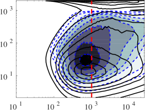
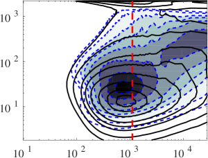
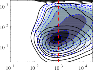
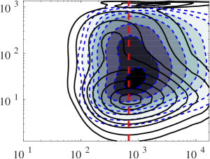
Figure 15: (Colour online) Maps of premultiplied one-dimensional energy spectra as function of streamwise wavelength $\lambda^{*}_{x}$ and distance from the wall $y^{*}$ at $Re=20\,000$ for $Ro=0$ (a, b), $Ro=0.15$ (c, d), $Ro=0.45$ (e, f) and $Ro=0.9$ (g, h). Left column shows $k_{x}\Phi_{uu}$ (black lines) and cospectra $k_{x}\Phi_{uv}$ (blue dashed lines and colours). Right column shows $k_{x}\Phi_{vv}$ (blue dashed lines and colours) and $k_{x}\Phi_{ww}$ (black lines). Contour levels from innermost to outermost are 0.94, 0.8, 0.6, 0.4, 0.28, 0.2, 0.1 and 0.05. Spectra are scaled with their maximum value.

At a higher $Ro=0.45$ the peaks in the spanwise spectra $k_{z}\Phi_{vv}$, $k_{z}\Phi_{ww}$ have, compared to the spectra at $Ro=0$, clearly shifted towards larger scales (figure 14.f) and these of the streamwise spectra $k_{x}\Phi_{vv}$, $k_{x}\Phi_{ww}$ to a streamwise wavelength $\lambda_{x}\approx 8\pi h/3$ (figure 15.f) in the outer layer. The energetic large-scale modes observed in the spanwise spectrum $k_{z}\Phi_{vv}$ at $\lambda_{z}\approx 3\pi h/8$ and $y\approx-0.5$ are not present at $Ro=0$, therefore, I interpret them as the signatures of roll cells. Two-point correlations, presented later, provide further evidence that they exist. The roll cells are smaller than at $Ro=0.15$ and do not appear to span the whole streamwise domain according to the streamwise spectra since the peak in the streamwise $k_{x}\Phi_{vv}$ is at $\lambda_{x}<L_{x}$. These observations are consistent with the results shown by the visualizations in figure 3 before. Dai et al. (2016) noted too that the roll cell diminished in size with $Ro$ in their DNS at a much lower $Re=2800$. In the present DNSs, energetic wide and long structures in terms of outer units are observed as well in the spanwise and streamwise spectra $\Phi_{uu}$ and especially the co-spectra $\Phi_{uv}$ at $Ro=0.45$ and even more so at $Ro=0.15$ in the outer layer (figure 14.c, e and 15.c, e), showing that the roll cells induce large-scale momentum transfer.

Previous studies have found strong support for the hypothesis that the logarithmic region of wall-bounded turbulent flows is populated by attached eddies (Perry & Chong 1982) whose size grows with $y$, see e.g. Smits et al. (2011) and Hwang (2015). Some evidence of attached eddies can indeed be found in the present spanwise spectrum $k_{z}\Phi_{uu}$ and cospectrum $k_{z}\Phi_{uv}$ of the non-rotating channel flow (figure 14.a) since they show that size of the structures grows with the distance to the wall in the logarithmic region. The cospectrum follows roughly the linear relation $y=0.2\lambda_{z}-1$ shown by the straight black dashed line in the figure, indicating that the size of eddies is approximately proportional to the distance to the wall, in agreement with the attached eddy hypothesis (Hwang 2015). The spanwise spectra $k_{z}\Phi_{uu}$ and cospectra $k_{z}\Phi_{uv}$ at $Ro=0.15$ and 0.45 (figure 14.c, e) show similar characteristics with growing scales as $y$ increases. The cospectrum follows also in these cases roughly the linear relation $y=0.2\lambda_{z}-1$. This provides support for the idea that also rotating wall-bounded flows are populated by attached eddies, at least up to moderate rotation rates.

At higher rotation rates large-scale structures become progressively less energetic and smaller. At $Ro=0.9$ no energetic large scale structures are seen in the spanwise spectra $k_{z}\Phi_{uu}$ and $k_{z}\Phi_{uv}$ while $k_{z}\Phi_{vv}$ has a peak at spanwise wavelength $\lambda_{z}\approx\pi h/6$ in the outer layer at $y\approx-0.8$ (figure 14.g and h). The streamwise spectrum of the streamwise velocity $k_{x}\Phi_{uu}$ has still a near-wall peak and that of the wall-normal velocity $k_{x}\Phi_{vv}$ has an outer peak at streamwise wave length $\lambda_{x}\approx 2\pi h/5$, while the spectrum of the spanwise velocity $k_{x}\Phi_{ww}$ has two energetic peaks: an outer peak at streamwise wave length $\lambda_{x}\approx\pi h/5$ and a near-wall peak at $\lambda_{x}\approx 4\pi h/5$ (figure 15.g and h). Energetic large-scale roll cells are thus not present according to the spectra and correspondingly, no large structures like roll cells are observed in visualizations and there are less energetic large-scale motions that contribute to momentum transfer than in a non-rotating channel flow.

Similar observations (not shown for brevity) are made at yet higher $Ro$, i.e., no energetic wide or long structures are present according to the spectra and co-spectra in terms of outer units. The peak in the spanwise spectrum $k_{z}\Phi_{vv}$ shifts towards shorter wavelengths and the double peak in the streamwise spectrum $k_{x}\Phi_{ww}$ persists. The double peak is also observed in the rms profiles (figure 6.c). The spanwise spectra $k_{z}\Phi_{uu}$ and $k_{z}\Phi_{uv}$ have still a spectral peak at $\lambda^{*}_{z}\approx 100$ but the peak moves closer to the wall in terms of viscous wall units. The streamwise spectra $k_{x}\Phi_{uu}$ and $k_{x}\Phi_{uv}$ have a spectral peak at $\lambda_{x}\approx h$ when $Ro\geq 0.9$, but in terms of the viscous wall units the structures become shorter. This means that the near-wall streaky structures move closer to the wall and become shorter, in agreement with the results of Lamballais et al. (1998), but they do not clearly confirm their finding that these structures become weaker at high $Ro$.

According to the spanwise spectrum $k_{z}\Phi_{uu}$ and cospectrum $k_{z}\Phi_{uv}$ at $Ro=0.9$ (figure 14.g) the structures do not become much larger when the distance to the wall increases and at higher $Ro$ the scales appear to grow even less with $y$. The absence of structures whose size grows with the distance to the walls when $Ro\gtrsim 0.9$ implies that attached eddies are much less prominent in very rapidly rotating wall-bounded flows. This suggests that the interaction between the inner and outer layer is weak at high $Ro$. Pressure and turbulent diffusion of turbulent kinetic energy are accordingly very small on the unstable side in that case.

Spectra at $Re=20\,000$ and $Ro=0.15$ at the stable side of the channel (not shown here) show that the roll cells observed on the unstable side do not deeply penetrate the stable channel side although the study by Dai et al. (2016) shows that they occasionally can become larger and may even affect the flow up to wall at the stable channel side. The spectra also show energetic near-wall modes at $\lambda^{*}_{z}\approx 100$ and $\lambda^{*}_{x}\approx 800$, as on the unstable side, implying that the near-wall cycle is maintained. On the other hand, although the flow is fully turbulent on the stable side at this low $Ro$, the spectra on the stable channel side reveal no or much less energetic large-scale modes than at $Ro=0$, showing that cyclonic rotation weakens large-scale structures in wall-bounded flows. This agrees with the observation that in plane Couette flow even very weak cyclonic spanwise rotation eliminates large-scale structures (Komminaho et al. 1996).

VII.2 Reynolds number dependence

In several other DNS studies of spanwise rotating channel flow large streamwise roll cells or Taylor-Görtler vortices have been found and examined, as mentioned before. Kristoffersen & Andersson (1993), Lamballais et al. (1998), Hsieh & Biringen (2016) and Dai et al. (2016) have observed them in DNSs at $Re_{\tau}\leq 200$ and $Ro\leq 0.5$. Hsieh & Biringen have observed them also at $Re_{\tau}=406$ and $Ro=0.2$. It is important that the roll cells are properly resolved since flow statistics deviate significantly if they are suppressed (Hsieh & Biringen 2016). Helical spectra computed from DNSs at $Re_{\tau}=180$ by Yang & Wu (2012) suggest large roll cells if $0.03\leq Ro\leq 0.57$ with the strongest signal at $Ro=0.15$. The size of the roll cells appears to diminish with $Ro$ for $Ro\geq 0.15$ and there is no sign that they exist at $Ro=0.94$ and higher. On the other hand, visualizations and spanwise two-point correlations computed by Grundestam et al. (2008) at $Re_{\tau}=180$ indicate that roll cells are present at $Ro=1.27$, but the statistics show that the roll cells are non-stationary and do not have a long correlation length in the streamwise direction and their size appears to be smaller than at lower $Ro$.

Thus, there is strong evidence that large roll cells exist in spanwise rotating channel flow at low Reynolds numbers for $Ro\lesssim 0.6$. At higher $Ro$ roll cells are less certain and more difficult to detect owing to their unsteadiness, but there are indications of their occurrence (Grundestam et al. 2008). Spectra presented before reveal large streamwise roll cells in a DNS at $Re=20\,000$ and $Ro=0.15$ and clearly hint at their occurrence at $Ro=0.45$, but at $Ro=0.9$ and higher there is no strong evidence of their presence. This suggests that at lower Reynolds numbers roll cells exist in a wider $Ro$ range. Note, that in previous DNSs of rotating channel flow the computational domain size was $4\pi\times 2\pi$ in the streamwise and spanwise direction, respectively, or less, which is smaller than in the present DNSs. This may influence the size and enhance the coherency of the roll cells, especially in combination with periodic boundary conditions. Indeed, in the DNS by Kristoffersen & Andersson (1993) at $Ro=0.15$ the roll cells were very steady whereas in the experiments by Johnston et al. (1972) the boundary conditions were different and the roll cells were much more unsteady.

To answer more unequivocally whether at low $Re$ roll cells exist in a wider $Ro$ range than at higher $Re$, I have computed premultiplied one-dimensional spanwise and streamwise spectra of the wall-normal and spanwise velocity fluctuations at $Re=5000$ for $Ro=0$, 0.15, 0.45 and 0.9, see figure 16.

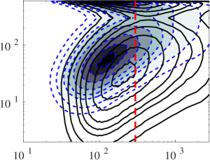
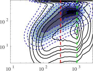
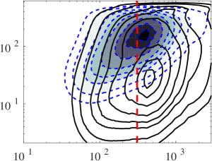
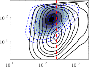
Figure 16: (Colour online) Maps of premultiplied one-dimensional spanwise and streamwise energy spectra at $Re=5000$ for $Ro=0$ (a, b), $Ro=0.15$ (c, d), $Ro=0.45$ (e, f) and $Ro=0.9$ (g, h). Left column shows spanwise spectra $k_{z}\Phi_{vv}$ (blue dashed lines and colours) and $k_{z}\Phi_{ww}$ (black lines). Right column shows streamwise spectra $k_{x}\Phi_{vv}$ (blue dashed lines and colours) and $k_{x}\Phi_{ww}$ (black lines). Contour levels from innermost to outermost are 0.94, 0.8, 0.6, 0.4, 0.28, 0.2, 0.1 and 0.05. Spectra are scaled with their maximum value.

The wavelength and the distance to the wall is, as in the previous spectra, scaled by the viscous length scale of the unstable side, $l^{*}=\nu/u_{\tau u}$, and the spectra are scaled with their maximum value, see table 2. The red dashed line marks again scales with a wavelength $h$. Spanwise two-point correlations of the wall-normal velocity fluctuations $R_{vv}=\overline{v(\mathbf{x}+z)v(\mathbf{x})}/\overline{vv}$ at $Re=3000$, 5000 and $20\,000$ and various $Ro$ have also been calculated. If streamwise vortices are present $R_{vv}$ is expected to display negative correlations with a minimum at a separation distance that is about equal to the mean vortex diameter. Accordingly, in non-rotating channel flow, $R_{vv}$ has a minimum at $z^{*}\approx 25$ near the wall as a result of near-wall streamwise vortices (Kim et al. 1987). The two-point correlations are shown at the unstable channel side at the wall-normal position where $R_{vv}$ approximately has the largest negative values and thus the signs of the roll cells are most clear. In all cases, the mean velocity profile is approximately linear at this position. The domain size is the same in all DNSs used to compute the spectra and two-point correlations.

At $Ro=0.15$ and $Re=5000$, the spanwise spectrum $k_{z}\Phi_{ww}$ has a peak at $\lambda_{z}=\pi h$ (indicated by the green dashed line) while the peak of $k_{z}\Phi_{vv}$ extends from about $\lambda_{z}=\pi h/2$ to $\pi h$ (figure 16.c) and the streamwise spectra reveal structures that span the whole streamwise domain (figure 16.d). Spectra at $Re=3000$ are not shown for brevity but at $Ro=0.15$ they show a peak at spanwise wave lengths $\lambda_{z}=\pi h$ and a lesser one at $3\pi h/5$. This indicates, similarly as at $Re=20\,000$, roll cells with a size of $\pi h/2$ and smaller ones. By comparing figure 16.(e) and (f) with figure 16.(a) and (b), it can be concluded that at $Ro=0.45$ wider and longer structures exist on the unstable channel side than at $Ro=0$, implying that large roll cells are present. The spectral peaks in the spanwise $k_{z}\Phi_{vv}$ and streamwise spectrum $k_{x}\Phi_{vv}$ are at $\lambda_{z}\approx 3\pi h/8$ and $\lambda_{x}\approx 2\pi h$, respectively. At similar wavelengths peaks are found in the spectra at $Re=20\,000$, as shown before, and $Re=3000$.

The spectra suggest that the roll cells at $Ro=0.15$ as well as at $Ro=0.45$ have a similar size for $Re=3000$ to $20\,000$. This is confirmed by the two-point correlations. At $Ro=0.15$, $R_{vv}$ is clearly negative for $0.5\lesssim z\lesssim 2$ and its minimum, which is a measure of the mean vortex diameter, is at about the same $z$ at all three Reynolds numbers (figure 17.a). The spectra suggest roll cells with a diameter $\pi h/2$ as well as smaller ones and that appears to be consistent with the two-point correlations which suggest roll cells with a mean diameter of about $h$. Also $R_{vv}$ at $Ro=0.45$ has a minimum at about the same $z$ at all three $Re$ (figure 17.b). The spectra indicate that the roll cells have a mean diameter of about $3\pi h/16$, in agreement with the two-point correlations.

These results indicate that for $Re=3000$ to $20\,000$ the size of the roll cells is smaller at $Ro=0.45$ than at $Ro=0.15$ but approximately independent of $Re$. The size $\pi h/2$ of the largest roll cells at $Ro=0.15$ indicated by the spanwise spectra is consistent with the size observed in the DNSs by Kristoffersen & Andersson (1993) and Yang & Wu (2012) at the same $Ro$. Yang & Wu also observed smaller roll cells and found that the size of the roll cells becomes smaller with $Ro$ for $Ro\geq 0.15$, again consistent with the present results. Also the DNSs by Dai et al. (2016) at $Re=2800$ show that the roll cells become smaller when $Ro$ increases from 0.1 to 0.5. On the other hand, the size $\pi h/2$ of the roll cells in the DNS by Hsieh & Biringen (2016) at $Ro=0.5$ and $Re_{\tau}\approx 200$ is considerably larger than in the present DNSs at $Ro=0.45$. This difference might be related to the more restricted computational domain used by Hsieh & Biringen. Besides, they only show visualizations of the time-averaged velocity field and these naturally emphasize the largest, most steady structures.

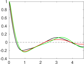
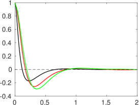
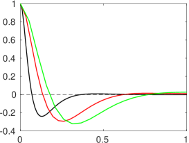
Figure 17: (Colour online) Spanwise two-point correlations of the wall-normal velocity fluctuations at (a) $Ro=0.15$ and $Re=20\,000$ and $y=-0.41$, $Re=5000$ and $y=0$, and $Re=3000$ and $y=0$; (b) $Ro=0.45$ and $Re=20\,000$ and $y=-0.54$, $Re=5000$ and $y=-0.55$, and $Re=3000$ and $y=-0.5$; (c, d) $Ro=0.9$ and $Re=20\,000$ and $y=-0.83$, $Re=5000$ and $y=-0.75$, and $Re=3000$ and $y=-0.75$; (e,f) $Ro=1.2$ and $Re=20\,000$ and $y=-0.92$, $Re=5000$ and $y=-0.83$, and $Re=3000$ and $y=-0.75$. In (a,b,c,e) $z$ is scaled by $h$ and in (d,f) $z^{*}=z/l^{*}$. (${\color[rgb]{0,0,0}~{}^{\line(1,0){20.0}}}$) $Re=20\,000$, (${\color[rgb]{1,0,0}~{}^{\line(1,0){20.0}}}$) $Re=5000$ and (${\color[rgb]{0,1,0}~{}^{\line(1,0){20.0}}}$) $Re=3000$.

At a higher $Ro=0.9$ the peak in the spanwise spectrum $k_{z}\Phi_{vv}$ shifts towards a smaller $\lambda_{z}\approx 3\pi h/13$ at $Re=5000$ (figure 16.g) and $\lambda_{z}\approx 3\pi h/11$ at $Re=3000$, which is at a larger wavelength than at $Re=20\,0000$ (figure 14.h). The large structures are also considerably longer in terms of outer units at lower $Re$, see figure figure 16.(h) vs. figure 15.(h). The minimum in $R_{vv}$ shift towards smaller $z$ at higher $Re$ (figure 17.c), confirming that at $Ro=0.9$ the large scales become smaller at higher $Re$. The two-point correlations (figure 17.e) and spectra (not shown here) show that at $Ro=1.2$ the differences are even more pronounced. The size of the large flow structures in terms of outer units shrinks monotonically with $Re$ and this trend continues at higher $Ro$. On the other hand, if the separation distance $z$ is scaled by the viscous length scale $l^{*}$ the two-point correlations differ considerably at $Ro=0.9$ (figure 17.d) and lower $Ro$ but much less at $Ro=1.2$ (figure 17.f) and higher $Ro$. The two-point correlations at $Re=3000$ and $Re=5000$ show in fact an almost perfect collapse. Thus, the size of the largest scales continues to decrease with $Ro$ but for $Ro\geq 0.9$ it becomes dependent of $Re$ as well. Whether these largest structures can be considered to be typical roll cells is not clear since the roll cells and typical near-wall streamwise vortices become less distinguishable at high $Ro$ and low $Re$. The two-point correlations suggest that their size start to display a viscous wall unit scaling and therefore may no have the same physical origin as at lower $Ro$.

VIII Conclusions

The present numerical study of fully developed plane turbulent channel flow subject to system rotation about the spanwise direction covers a wide range of parameters with $Re$ between 3000 and $31\,600$ and $Ro$ between 0 and 2.7. At all $Re$ and for a wide range of $Ro$ the mean streamwise velocity profile has a linear part with a slope $\mbox{d}U/\mbox{d}y\simeq 2\Omega$ implying that this mean zero-absolute-vorticity state is independent of the Reynolds number. This zero-absolute-vorticity state has also been found in low-Reynolds number and approximately in transitional rotating channel flow (Iida et al. 2010, Wall & Nagata 2013) and in laminar and turbulent plane Couette flow subject to anticyclonic rotation (Kawata & Alfredsson 2016, Gai et al. 2016). In all these other cases, the flow is dominated by large streamwise roll cells. Hsieh & Biringen (2016) found that when roll cells are suppressed in DNSs of rotating turbulent channel flow by decreasing the spanwise domain size the slope of the mean velocity profile $\mbox{d}U/\mbox{d}y$ deviates from $2\Omega$ pointing out that it is important to resolve the roll cells. In the present study, the zero-absolute-vorticity state exists too at high $Ro$ when the flow is turbulent but roll cells are absent or small proving that roll cells are not a prerequisite. Some possible explanations for the zero-absolute-vorticity state have been proposed (Hamba 2006, Kawata & Alfredsson 2016) but none rigorous. Because of the linear mean velocity slope, profiles of the production and dissipation rate of turbulent kinetic energy and some of the budget terms in the Reynolds stress equations show a linear part as well. In this part of the unstable channel side, basically all energy is fed into the wall-normal Reynolds stress component when the production and Coriolis term are considered together. The energy is then redistributed to the streamwise and especially the spanwise Reynolds stress component through pressure-strain correlations.

Through visualizations, one-dimensional spectra and two-point correlations the influence on rotation on turbulence structures is investigated. A distinct unstable side with intense turbulence and vortical structures and a stable side with much weaker turbulence develops in the channel with an apparent sharp border between the two sides. If $Ro$ approaches 0.45 the flow at higher $Re$ partly relaminarizes on the stable side of the channel and oblique turbulent-laminar patterns develop which resemble the oblique band-like structures found in transitional Couette and channel flows at low Reynolds numbers (Duguet et al. 2010, Tuckerman et al. 2014). It is quite remarkable that such patterns exist in rotating channel flow at a significantly higher $Re$. The study by Brethouwer et al. (2012) suggests that turbulent-laminar patterns similar to those found in my DNS at $Ro=0.45$ and $Re=20\,000$ to $31\,600$ also exist at lower $Re$ but at a lower $Ro$ and that the patterns most likely have a longer wave length at lower $Re$. This implies that the patterns may appear at low $Re$ in DNSs of rotating channel flow if very larger computational domains are used.

If $Ro$ is raised further in the present DNSs the turbulent fraction of the flow on the stable side goes down and eventually the flow relaminarizes there. The unstable part of the channel with strong turbulence diminishes in size with $Ro$ and when the rotation rate is sufficiently high the whole flow becomes laminar. However, as shown by Brethouwer (2016), a linear instability can develop in rapidly rotating channel flows causing a continuous cycle of turbulent bursts.

The influence of $Re$ is investigated and found to be significant. At fixed $Ro$ Reynolds stresses are noticeably stronger on the stable side of the channel at higher $Re$. When $Ro\leq 0.9$, the flow is partly or fully turbulent on the stable channel side at higher $Re$ whereas at lower $Re$ the turbulent fraction of the flow is significantly smaller and the flow tends to relaminarize faster. Care has therefore has to be exercised when drawing general conclusions from lower Reynolds number studies of rotating channel flow. Attention should also be paid to the size of the computational domain since that may have a significant influence on the large-scale structures like roll cells and the relaminarization of the stable channel side.

On the unstable side of the channel, large counter-rotating streamwise roll cells are observed at $Ro=0.15$ and 0.45. The roll cells become smaller and less noticeable and eventually disappear if $Ro$ is raised. This trend is stronger at higher $Re$ since at high $Ro$ the large-scale modes, which are possibly related to roll cells, are larger at lower $Re$. This suggests that at low $Re$ roll cells may exist in a wider $Ro$ range, but note there is yet no way to unambiguously determine if roll cells exists. The spectra also indicate that at lower $Ro$ the unstable channel side is populated by attached eddies whereas these appear to be absent at higher $Ro$, indicating that the interaction between the inner and outer layer is weak in rapidly rotating channel flows.

The present case gives some general insights into the effect of rotation on wall-bounded flows. It is valuable as well for turbulence modelling since the influence of rotation is turbulence is still difficult to model. Even for large-eddy simulation it could be a demanding case because correctly predicting the relaminarization of rapidly rotating channel flow may pose a challenge.

- (1) Adrian, R.J. 2007 Hairpin vortex organization in wall turbulence. Phys. Fluids 19, 041301.
- (2) Agostini, L., Leschziner, M. 2016 Predicting the response of small-scale near-wall turbulence to large-scaleouter motions. Phys. Fluids 28, 015107.
- (3) Alvelius, K. 1999 Studies of turbulence and its modelling through large eddy- and direct numerical simulations. PhD thesis, Department of Mechanics, KTH, Stockholm, Sweden.
- (4) Arolla, S.K. & Durbin, P.A. 2013 Modeling rotation and curvature effects within scalar eddy viscosity model framework. Int. J. Heat Fluid Flow 39, 78–89.
- (5) Barkley, D. & Tuckerman, L. S. 2007 Mean flow of turbulent-laminar patterns in plane Couette flow. J. Fluid Mech. 576, 109–137.
- (6) Brethouwer, G. 2005 The effect of rotation on rapidly sheared homogeneous turbulence and passive scalar transport. Linear theory and direct numerical simulations. J. Fluid Mech. 542, 305–342.
- (7) Brethouwer, G. 2016 Linear instabilities and recurring bursts of turbulence in rotating channel flow simulations. Phys. Rev. Fluids 1, 054404.
- (8) Brethouwer, G., Duguet, Y., Schlatter, P. 2012 Turbulent-laminar coexistence in wall flows with Coriolis, buoyancy or Lorentz forces. J. Fluid Mech. 704, 137–172.
- (9) Brethouwer, G., Schlatter, P., Duguet, Y., Henningson, D.H., Johansson. A.V. 2014 Recurrent bursts via linear processes in turbulent environments. Phys. Rev. Lett. 112, 144502.
- (10) Chevalier, M., Schlatter, P., Lundbladh, A. & Henningson, D. S. 2007 A pseudo-spectral solver for incompressible boundary layer flows. Technical Report TRITA-MEK 2007:07, KTH Mechanics, Stockholm, Sweden.
- (11) Christensen, K.T. & Adrian, R.J. 2001 Statistical evidende of hairpin vortex packets in wall turbulence. J. Fluid Mech. 431, 433–443.
- (12) Dai, Y.-J., Huang, W.-X., Xu, C.-X. 2016 Effects of Taylor-Görtler vortices on turbulent flows in a spanwise-rotating channel. Phys. Fluids 28, 115104.
- (13) Deusebio, E., Brethouwer, G., Schlatter, P., Lindborg, E. 2014 A numerical study of the stratified and unstratified Ekman layer. J. Fluid Mech. 755, 672–704.
- (14) Deusebio, E., Caulfield, C. P., Taylor, J. R. 2015 The intermittency boundary in stratified plane Couette flow. J. Fluid Mech. 781, 298–329.
- (15) Duguet, Y., Schlatter, P. 2013 Oblique laminar-turbulent interfaces in plane shear flows. Phys. Rev. Lett. 110, 034502.
- (16) Duguet, Y., Schlatter, P. & Henningson, D. S. 2009 Formation of turbulent patterns near the onset of transition in plane Couette flow. J. Fluid Mech. 650, 119–129.
- (17) Gai, J., Xia, Z., Cai, Q., Chen, S. 2016 Turbulent statistics and flow structures in spanwise-rotating turbulent plane Couette flows. Phys. Rev. Fluids 1, 054401.
- (18) Garcia-Villalba, M., del Álamo, J. C. 2011 Turbulence modification by stable stratification in channel flow. Phys. Fluids 23, 045104.
- (19) Grundestam, 0., Wallin, S., Johansson, A.V. 2008 Direct numerical simulations of rotating turbulent channel flow. J. Fluid Mech. 598, 177–199.
- (20) Hamba, F. 2006 The mechanism of zero absolute vorticity statte in rotating channel flow. Phys. Fluids 18, 125104.
- (21) Hsieh, A., Biringen, S. 2016 The minimal flow unit in complex turbulent flows. Phys. Fluids 28, 125102.
- (22) Hsieh, A., Biringen, S., Kucala, A. 2016 Simulation of rotating channel flow with heat transfer: evaluation of closure models. ASME J. Turbomach. 138, 111009.
- (23) Hwang, Y. 2015 Statistical structure of self-sustaining attahced eddies in turbulent channel flow. J. Fluid Mech. 767, 254–289.
- (24) Iida, O., Fukudome, K., Iwata, T., Nagano, Y. 2010 Low Reynolds number effects on rotating turbulent Poiseuille flow. Phys. Fluids 22, 085106.
- (25) Jakirlić, S., Hanjalić, K., Tropea, C. 2002 Modeling rotating and swirling turbulent flows: a perpetual challenge. AIAA J. 40, 1984.
- (26) Jeong, J., Hussain, F. 1995 On the identification of a vortex. J. Fluid Mech. 285, 69–94.
- (27) Johnston, J.P., Halleen, R.M., Lezius, D.K. 1972 Effects of spanwise rotation on the structure of two-dimensional fully developed turbulent channel flow. J. Fluid Mech. 56, 533–559.
- (28) Kawata, T., Alfredsson, P.H. 2016 Experiments in rotating plane Couette flow – momentum transport by coherent roll-cell structure and zero-absolute-vorticity state. J. Fluid Mech. 791, 191–213.
- (29) Kim, J., Moin, P., Moser, R. 1987 Turbulence statistics in fully developed channel flow at low Reynolds number. J. Fluid Mech. 177, 133–166.
- (30) Komminaho, J., Lundbladh, A., Johansson, A.V. 1996 Very large structures in plane turbulent Couette flow. J. Fluid Mech. 320, 259–285.
- (31) Kristoffersen R., Andersson, H.I. 1993 Direct simulations of low-Reynolds number turbulent flow in a rotating channel. J. Fluid Mech. 256, 163–197.
- (32) Lamballais, E., Lesieur, M., Métais, O. 1996 Effects of spanwise rotation on the vorticity stretching in transitional and turbulent channel flow. Int. J. Heat Fluid Flow 17, 324–332.
- (33) Lamballais, E., Métais, O., Lesieur, M. 1998 Spectral-dynamic model for large-eddy simulations of turbulent rotating channel flow. Theor. Comput. Fluid Dyn. 12, 149–177.
- (34) Lee, M., Moser, R.D. 2015 Direct numerical simulation of turbulent channel flow up to . J. Fluid Mech. 774, 395–415.
- (35) Lenaers, P., Li, Q., Brethouwer, G., Schlatter, P., Örlü, R. 2012 Rare backflow and extreme wall-normal velocity fluctuations in near-wall turbulence. Phys. Fluids 24, 035110.
- (36) Liu, N.-S., Lu, X.-Y. 2007 Direct numerical simulation of spanwise rotating turbulent channel flow with heat transfer. Int. J. Numer. Meth. Fluids 53, 1689–1706.
- (37) Marstorp, L., Brethouwer, G., Grundestam, O., Johansson, A.V. 2009 Explicit algebraic subgrid stress models with application to rotating channel flow. J. Fluid Mech. 639, 403–432.
- (38) Mathis, R., Hutchins, N., and Marusic, I. 2009 Large-scale amplitude modulation of the small-scale structures in turbulent boundary layers J. Fluid Mech. 628, 311–337.
- (39) Monty, J.P., Hutchins, N., Ng, H.C.H., Marusic, I., Chong, M.S. 2009 A comparison of turbulent pipe, channel and boundary layer flows. J. Fluid Mech. 632, 431–442.
- (40) Nagano, Y., Hattori, H. 2003 Direct numerical simulation and modelling of spanwise rotating channel flow with heat transfer. J. Turbulence 4, 010.
- (41) Nakabayashi, K., and Kitoh, O. 2005 Turbulence characteristics of two-dimensional channel flow with system rotation, J. Fluid Mech. 528, 355–377.
- (42) Perry, A.E., Chong, M.S. 1982 On the mechanism of wall turbulence. J. Fluid Mech. 119, 173–217.
- (43) Salhi, A., Cambon, C. 1997 An analysis of rotating shear flow using linear theory and DNS and LES results. J. Fluid Mech. 347, 171–195.
- (44) Schmid, P.J., Henningson, D.S. 2001 Stability and transition in shear flows, Applied Mathematical Sciences 142, Springer.
- (45) Smirnov, P.E., Menter, F.R. 2009 Sensitization of the SST turbulence model to rotation and curvature by applying the Spalart-Shur correction. ASME J. Turbomach. 131, 041010.
- (46) Smits, A.J.,McKeon, B.J., and Marusic, I. 2011 High-Reynolds number wall turbulence. Ann. Rev. Fluid Mech. 43, 353–375.
- (47) Talluru, K.M., Baidya, R., Hutchins, N., Marusic, I. 2014 Amplitude modulation of all three velocity components in turbulent boundary layers. J. Fluid Mech. 746., R1.
- (48) Tritton, D.J. 1992 Stabilization and destablization of turbulent shear flow in a rotating fluid. J. Fluid Mech. 241, 503–523.
- (49) Tuckerman, L.S., Kreilos, T., Schrobsdorff, H., Schneider, T.M., Gibson, J.F. 2014 Turbulent-laminar patterns in plane Poiseuille flow. Phys. Fluids 26, 114103.
- (50) Wall, D.P., Nagata, M. 2013 Three-dimensional exact coherent states in rotating channel flow. J. Fluid Mech. 727, 533–581.
- (51) Wallin, S., Grundestam, O., Johansson, A.V. 2013 Laminarization mechanisms and extreme-amplitude states in rapidly rotating plane channel flow. J. Fluid Mech. 730, 193–219.
- (52) Xia, Z., Shi, Y., Chen, S. 2016 Direct numerical of turbulent channel flow with spanwise rotation. J. Fluid Mech. 788, 42–56.
- (53) Yang, Z.X., Cui, G.X., Zhang, Z.S., Xu, C.X. 2012 A modified nonlinear sub-grid scale model for large eddy simulation with application to rotating turbulent channel flows. Phys. Fluids 24, 075113.
- (54) Yang, Y.-T., Wu, J.-Z. 2012 Channel turbulence with spanwise rotation studied using helical wave decomposition. J. Fluid Mech. 692, 137–152.