Stellar dynamo models with prominent surface toroidal fields

Abstract

Recent spectro-polarimetric observations of solar-type stars have shown the presence of photospheric magnetic fields with a predominant toroidal component. If the external field is assumed to be current-free it is impossible to explain these observations within the framework of standard mean-field dynamo theory. In this work it will be shown that if the coronal field of these stars is assumed to be harmonic, the underlying stellar dynamo mechanism can support photospheric magnetic fields with a prominent toroidal component even in the presence of axisymmetric magnetic topologies. In particular it is argued that the observed increase in the toroidal energy in low mass fast rotating stars can be naturally explained with an underlying $\alpha\Omega$ mechanism.

1 Introduction

One of the most compelling problems in modern dynamo theory is the formulation of a realistic coupling between the internal magnetic field and the external field in the atmosphere. In fact the boundary conditions for the electric and the magnetic field at the stellar surface put severe constraints on the allowed coronal field configurations, and it is often necessary to resort to very crude approximations for the latter.

The standard textbook boundary condition employed in mean-field dynamo theory amounts to consider a current-free field in the region $r\geq R$ where $R$ is the stellar radius, so that $\nabla\times\mathbf{B}=0$ in this domain. Although in the solar case this assumption is motivated by the possibility of describing the almost rigid rotation of the coronal holes in the lower corona (Nash et al., 1988), it be might incorrect to extend its validity in more active stars.

In fact, as current-free fields represents the states of minimum energy under the constraint that the normal component of the field at the photosphere is fixed, they cannot provide the additional energy required to sustain a significant activity level. Recent measurements of Faraday rotation in the solar corona support the evidence for large scale coronal currents (Spangler, 2007), an essential ingredient to explain coronal heating in terms of Joule dissipation. On the other hand on much smaller scales the presence of currents is unavoidable in order to explain the twisted field structure of filaments and prominences.

Force-free magnetic fields, defined by $\nabla\times\mathbf{B}=\alpha_{ff}(\mathbf{x})\mathbf{B}$ where $\alpha_{ff}(\mathbf{x})$ is a scalar function, can be more appealing from the physical point of view, at least for very low plasma-$\beta$ values. However, recent investigations based on direct numerical simulations have shown that the free magnetic energy and the efficiency of coronal heating via currents dissipation are still very limited in these models (Peter et al., 2015).

An important consequence of current-free boundary conditions is that the toroidal field must identically vanish in the all domain $r\geq R$. In order to illustrate this point in detail it is convenient to introduce the scalar potential $\Phi(r,\vartheta,\varphi)$ so that the toroidal field can be written as

$$\boldsymbol{B}_{\rm T}=-\frac{1}{\sin\theta}\frac{\partial\Phi}{\partial\varphi}\mathbf{e}_{\vartheta}+\frac{\partial\Phi}{\partial\vartheta}\mathbf{e}_{\varphi}.$$ (1)

It is not difficult to show that, if $\Phi$ is a single valued function, $\nabla\times\boldsymbol{B}_{\rm T}=0$ in a volume always necessarily implies $\boldsymbol{B}_{\rm T}\equiv 0$ everywhere (Krause & Raedler, 1980). In particular, if the field configuration is spherically symmetric the azimuthal component of the magnetic field must vanish at the surface, so that $\frac{\partial\Phi}{\partial\vartheta}|_{r=R}=0$, as imposed in most of the dynamo models (see Moss & Sokoloff (2009) for an interesting discussion on this issue).

Spectropolarimetric observations of photospheric magnetic fields in solar-like stars have revealed surface toroidal field which are mostly axysimmetric and have a predominant toroidal component (Petit et al., 2005, 2008; Fares et al., 2010, 2013; See et al., 2015) implying that most of the magnetic energy resides in the toroidal field. This is the case of the solar-like stars like HD72905, with 82% of the magnetic energy stored in the toroidal field which is nearly completely axisymmetric (97%), or of the G8 dwarf $\xi$ Boo A with 81% of toroidal energy of which 97% is due to the axisymmetric component, or the case of HD56124 with 90% of the energy in axisymmetric field configurations, and roughly the same strength of poloidal and toroidal component. The situation is even more dramatic if one considers M dwarfs like WX UMa or AD Leo where nearly all the energy is stored in an axysymmetric field with prominent photospheric non-zero toroidal component (see See et al. (2015) for a detailed discussion).

While in the case of the Sun a similar observational strategy has confirmed that the magnetic energy is mostly ($>90$%) poloidal (Vidotto, 2016), it is clear that the boundary conditions based on current-free coronal field might not be correct for other, more active, stars. In fact it has been further noticed that fast rotating, low mass stars have on average stronger surface toroidal fields than solar-mass slow rotators (See et al., 2016). Can this fact be explained as an enhanced dynamo action due a $\alpha\Omega$ mechanism? Indeed, as strong toroidal fields can alter the average atmospheric structure there is no reason to assume that a current-free field is still a reasonable approximation to discuss the magnetic energy budget in these objects.

The idea proposed in this paper is that on large scales and on time scales of the order of the stellar cycle, the external field can be considered harmonic so that:

$$\nabla^{2}\mathbf{B}+k^{2}\mathbf{B}=0$$ (2)

where the wavenumber $k$, assumed to be real, determines the characteristic spatial length of the field.

As it is well known, in the Sun various MHD instabilities trigger multiple modes harmonics on different length scales (Nakariakov & Verwichte, 2005; Arregui et al., 2013). In more active stars one can thus argue that the dynamo waves from the interior trigger global oscillations of the coronal field which then propagate according to (2).

It is important to remark that linear force-free fields with $\alpha_{ff}^{2}=k^{2}$ are solutions of (2) (notice that strictly speaking $\alpha_{ff}$ is a pseudoscalar while $k$ is a scalar), although the converse is not true in general (Chandrasekhar & Kendall, 1957). In this investigation it turns out that the coronal fields obtained by coupling (2) with dynamo solutions in the interior are approximately force-free in the sense of Warnecke & Brandenburg (2010) as $\langle(\mathbf{J}\times\mathbf{B})^{2}\rangle\ll\langle\mathbf{B}^{2}\rangle\langle\mathbf{J}^{2}\rangle$.

It will then be shown that standard MHD continuity conditions at the surface naturally allow for non-zero surface toroidal fields which is directly extrapolated from the interior field produced by the dynamo. In this letter several solutions obtained for solar-like stars will therefore be discussed and analyzed. It turns out that depending on the strength of the differential rotation and the surface meridional circulation, it is possible to obtain surface fields whose energies distribution between toroidal and poloidal components is consistent with the observations.

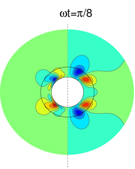
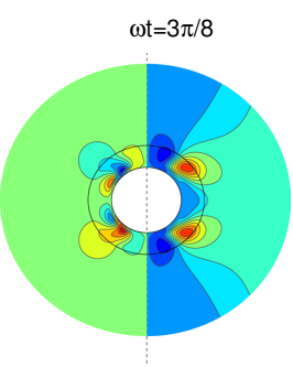
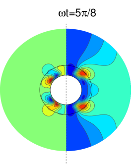
Figure 1: Temporal evolution of the global (interior+corona) solution for model J of table (1). The left hemisphere represents the isocontour lines of the toroidal field with blue levels for negative $B_{\varphi}$ and red for positive values of the field. The right hemisphere represents the streamlines of the poloidal field. Blue levels are for counterclockwise field lines, red levels for clockwise field lines. Notice the opening of the field lines at $2R$.

2 Basic equations

Let us assume that the field periodically evolves with a characteristic cycle frequency $\omega$ so that $\mathbf{B}=e^{-i\omega t}\boldsymbol{\mathcal{B}}$. Eq. (2) thus reads

$$(\nabla^{2}+k^{2})\boldsymbol{\mathcal{B}}=0$$ (3)

where the wavenumber $k$ is considered to be real. Clearly we must assume that $Rk\ll 1$ otherwise the typical spatial structure of the field would be too short to be consistent with our quasi-homogeneous approximation. As we shall see, as long as $Rk\ll 1$ our results are not quantitatively dependent on the value of $k$.

As usual, the boundary conditions are the continuity of the normal component of the magnetic field and the tangential component of the electric field across the stellar surface,

$$[[\mathbf{n}\cdot\mathbf{B}]]=0,\;\;[[\mathbf{n}\times\mathbf{E}]]=0$$ (4)

where $\mathbf{n}$ is the normal to the surface. In spherical symmetry the following decomposition for the magnetic field $\boldsymbol{\mathcal{B}}$ can be used

$$\boldsymbol{\mathcal{B}}=-\mathbf{r}\times\nabla\Psi-\nabla\times(\mathbf{r}\times\nabla\Phi)\equiv\boldsymbol{\mathcal{B}}_{\rm T}+\boldsymbol{\mathcal{B}}_{\rm P}$$ (5)

where $\Psi=\Psi(r,\vartheta,\varphi)$ and $\Phi=\Phi(r,\vartheta,\varphi)$ are scalar functions, $\boldsymbol{\mathcal{B}}_{\rm T}$ is the toroidal component and $\boldsymbol{\mathcal{B}}_{\rm P}$ is the poloidal one (see Krause & Raedler (1980) for details). The vector Helmholtz equation (3) decouples in the two scalar equations

$$\nabla^{2}\Phi+k^{2}\Phi=0$$ (6a)

$$\nabla^{2}\Psi+k^{2}\Psi=0$$ (6b)

and variable separation in (6) gives

$$\Phi=R\sum_{n}^{\infty}[A_{n}j_{n}{(\xi x)}+B_{n}y_{n}(\xi x)]P_{n}(\cos\theta)$$ (7a)

$$\Psi=\sum_{n}^{\infty}[C_{n}j_{n}{(\xi x)}+D_{n}y_{n}(\xi x)]P_{n}(\cos\theta)$$ (7b)

where $x$ is the normalized stellar radius $x=r/R$, $\xi=kR$, $P_{m}(\cos\theta)$ are the Legendre polynomials and $j_{n}(x)$ and $y_{n}(x)$ are the spherical Bessel functions. It should be remarked that $k=0$ in (6) does not necessarily imply $\Psi\equiv 0$ in the all $r\geq R$ domain, as it must instead hold in the case of a current-free field (vacuum boundary condition).

The $A_{n}$-$D_{n}$ constants are complex numbers whose value must be determined by the boundary conditions (4) imposed at the stellar surface and at some finite outer radius $r=R_{\rm out}$ where a transition to a wind dominated field topology occur (Parker, 1958). For our purposes it will be sufficient to assume that at $r=R_{\rm out}$ the solution is radially dominated so that

$$B_{\theta}(r=R_{\rm out})=B_{\phi}(r=R_{\rm out})=0.$$ (8)

In the stellar interior the field is described by the mean-field dynamo equation

$$\frac{\partial\mathbf{B}}{\partial t}=\nabla\times(\mathbf{U}\times\mathbf{B}+\alpha\mathbf{B})-\nabla\times(\eta\nabla\times\mathbf{B})$$ (9)

where, as usual, $\alpha$ is a pseudo-scalar function representing the turbulent $\alpha$-effect, $\mathbf{U}$ is the mean flow and $\eta$ is the turbulent (eddy) diffusivity. As before $\mathbf{B}=e^{-i\omega t}\boldsymbol{\mathcal{B}}$ and we apply the fundamental decomposition (5) for $\boldsymbol{\mathcal{B}}$. At last we write

$$\Phi=R\sum_{n}^{\infty}\phi_{n}(x)P_{n}(\cos\theta)$$ (10a)

$$\Psi=\sum_{n}^{\infty}\psi_{n}(x)P_{n}(\cos\theta)$$ (10b)

where $\psi_{n}$ and $\phi_{n}$ are the complex eigenfunctions of antisymmetric parity of the linear operator (9) (see Rädler (1973) for details).

The field at the inner boundary is assumed to be a perfect conductor, but the boundary conditions (4) at the surface imply the continuity of $\phi_{n}$, $\psi_{n}$ and their derivatives across the boundary. It is not difficult to show that, in order for the interior solution to be consistent with the external field in (7) the following relation must hold at $x=1$ :

$$\frac{d\phi_{n}}{dx}+\left[\frac{\gamma_{n}y_{n+3/2}(\xi)+j_{n+3/2}(\xi)}{\gamma_{n}y_{n+1/2}(\xi)+j_{n+1/2}(\xi)}-n\right]\phi_{n}=0$$ (11)

where $\gamma_{n}=A_{n}/B_{n}$ are determined by imposing the outer boundary condition (8) on $r=R_{\rm out}$. A similar equation can be obtained for the $\psi_{n}$ components.

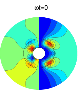
Figure 2: Same as model J but with a convection zone which extends from $x=0.5$. In this case $C_{\alpha}=7.86$, $C_{\omega}=49.5$ and $E_{\rm T}/E_{\rm tot}=0.90$.

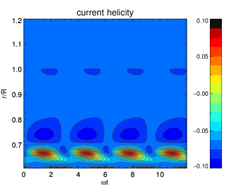
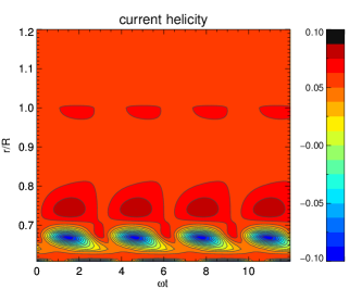
Figure 3: Upper panel: evolution of $\mu_{0}R\mathbf{J}\cdot\mathbf{B}/\langle\mathbf{B}^{2}\rangle$ computed at +30^∘ latitude for a $\alpha^{2}\Omega$ advection dominated solar dynamo model with $kR=0.1$, $C_{\alpha}=3.03$, $C_{\Omega}=3\cdot 10^{4}$, $C_{u}=400$ and the cycle period is 32 years. Lower panel: same model as upper panel but opposite hemisphere. Notice that the helicity changes sign from the turbulent zone in the interior, to the exterior.

3 Dynamo models

Let us specialize our formalism to the case of a solar-like star. We assume the following form for the velocity field $\mathbf{U}=\mathbf{u}(r,\theta)+r\sin\theta\Omega(r,\theta)\mathbf{e}_{\phi}$ and we model the solar-like differential rotation in the following way:

$$\Omega(r,\theta)=\Omega_{c}+\frac{1}{2}\left[1+{\rm erf}\left(\frac{x-x_{c}}{d}\right)\right](\Omega_{s}(\theta)-\Omega_{c})$$ (12)

where $x_{c}$ is the location of the convection zone in units of the stellar radius, $d=0.02$, $\Omega_{c}$ is the uniform angular velocity of the radiative core, $\Omega_{s}(\theta)=\Omega_{0}-d\Omega\cos^{2}\theta$. Here $d\Omega=\Omega_{eq}-\Omega_{c}$ is the surface differential rotation (in principle obtained from observations). For actual calculations we fixed $x_{c}=0.7$ and $\Omega_{c}/\Omega_{eq}=0.9$ but $d\Omega/\Omega_{eq}$ is allowed to vary. The radial profile of the turbulent diffusivity is assumed to be the following:

$$\eta=\eta_{c}+\frac{1}{2}(\eta_{t}-\eta_{c})\left[1+{\rm erf}\left(\frac{x-x_{x}}{d}\right)\right]$$ (13)

with $\eta_{c}/\eta_{t}=10^{-1}$. The $\alpha$ effect is proportional to $\cos\vartheta$ and its radial profile is assumed to be uniformly distributed in all the convection zone (see Bonanno et al. (2002) for details). The meridional circulation $\mathbf{u}$ is obtained from the stream function $S(r)$ which as explained in Bonanno (2013) $S(r)$ can be obtained from an underlying stellar model. The flow as usual is equatorwards at the equator and poleward at the surface.

As usual, let us introduce the following dynamo numbers, $C_{\Omega}={R^{2}\Omega_{0}}/{\eta_{t}}$, $C_{\alpha}={R\alpha_{0}}/{\eta_{t}}$, $C_{u}={RU_{0}}/{\eta_{t}}$, $C_{\omega}={R^{2}\omega}/{\eta_{t}}$ where $\Omega_{0}$ is the rotation rate at the equator and $U_{0}$ is the maximumm strength of $u_{\theta}$ at the bottom of the convection zone. The resulting eigenvalue problem can be conveniently solved by inverting a block-diagonal complex matrix (Rädler, 1973; Bonanno, 2013) which must be truncated to the desired numerical accuracy. For calculations we used the kinematic dynamo code CTDYN, developed by the author and extensively tested in Jouve et al. (2010). Our results are summarized in table (1).

${\cal M}$	$C_{\Omega}$	$C_{u}$	$d\Omega/\Omega_{eq}$	$kR$	$C_{\alpha}$	$C_{\omega}$	$E_{\rm T}/E_{\rm tot}$
A	1000	0	0.1	0.1	7.87	$\infty$	0.67
B	1000	0	0.1	0.4	7.88	$\infty$	0.67
C	1000	0	0.3	0.1	11.24	$\infty$	0.67
D	1000	100	0.3	0.1	7.78	$\infty$	0.37
E	2000	0	0.1	0.1	9.49	$\infty$	0.63
F	2000	0	0.3	0.1	10.97	79.02	0.91
G	2000	0	0.3	vac	11.94	69.98	0
J	4000	0	0.1	0.1	10.11	62.93	0.85
K	4000	0	0.1	0.5	10.04	63.03	0.86
L	4000	100	0.1	0.1	5.57	$\infty$	0.68
M	4000	200	0.1	0.1	5.13	$\infty$	0.37

Table 1: Summary of the numerical simulations. In particular it shows how $E_{\rm T}/E_{\rm tot}$ depends on $C_{\Omega}$ and various other input parameters (“vac” stands for current-free boundary condition). ${\cal M}$ is the model name, and in particular for model J the toroidal and poloidal field are displayed in fig. (1) at various values of the cycle phase.

Let us first stress that the $E_{\rm T}/E_{\rm tot}$ at the surface is non-zero and it is now an increasing function of $C_{\Omega}$, an effect clearly expected for an $\alpha\Omega$ dynamo. The surface differential rotation also plays an important role because it strongly influences the value of $E_{\rm T}/E_{\rm tot}$, as it can be deduced by looking at models E and F for instance. On the contrary, it should also be noticed the decrease of $E_{\rm T}/E_{\rm tot}$ as the flow is increased (see models J, L, M for instance). This fact has a clear physical interpretation: as the flow is poleward below the surface, the toroidal belts become more and more confined below the surface at high $C_{u}$. It is also reassuring to notice that, as long as $kR\ll 1$ our results are not sensitive to the choice of $\xi$. On the other hand, with the new boundary conditions the value of the critical $C_{\alpha}$ is in general smaller than with the standard current-free boundary conditions as it can be observed by looking at models F and G. We also verified that our results are not qualitatively dependent on the location of the external boundary $R_{\rm out}$. Moreover, low mass stars with more extended convection zone have in general higher values of $E_{\rm T}/E_{\rm tot}$, if $C_{\Omega}$ is large enough, as discussed in the model of fig. (2).

If the dynamo action is instead driven by the meridional circulation (as in mean field models of the solar dynamo) the new boundary condition does not alter the internal dynamo action because the toroidal field is localized at the bottom of the convection zone.

In the case of a generic $\alpha\Omega$ advection-dominated dynamo action we observe a change of sign of the dimensionless ratio $\mathbf{J}\cdot\mathbf{B}/\langle\mathbf{B}^{2}\rangle$ from positive (in the norther hemisphere) in the turbulent zone in the interior to negative in the exterior. The opposite happens in the southern hemisphere as one can see in fig. (3). A similar change of sign between the turbulent zone and the exterior has also been observed in (Warnecke et al., 2011), although in our mean-field models the current helicity is mostly negative in the outer layers in the norther hemisphere.

4 conclusions

The description of the external field in terms of solution of the Helmholtz equation allowed us to extrapolate the internal toroidal field generated by the dynamo on the photosphere, and finally to make contact with the observations. The assumption beyond this idea is the possibility of treating the corona as an external passive medium with effective macroscopic dielectric properties, if averaged over long enough time scales. Although this approach oversimplifies the complex physics of the corona, in our opinion it represents a significant improvement of the current-free boundary conditions for which $\boldsymbol{B}_{\rm T}\equiv 0$ on the surface, at least in some class of very active stars. The resulting dynamo numbers are in general smaller than the standard critical dynamo numbers; the ratio $E_{\rm T}/E_{\rm tot}$ increases with $C_{\Omega}$ and with a more extended convection zone, and decreases with $C_{u}$. Indeed, fast rotating stars with larger convection zone should approach a cylindrical rotation law in the interior with a smaller surface meridional circulation.

One can therefore argue that the general increase of the surface toroidal energy in low mass fast rotating stars finds its natural explanation in an underlying $\alpha\Omega$ dynamo mechanism.

A detailed study of all the parameter space and a comparison with the global topologies inferred from observations will be discussed in a longer paper. We also plan to extend this investigation including non-axisymmetric solutions of higher azimuthal modes.

References

- Arregui et al. (2013) Arregui, I., Asensio Ramos, A., & Díaz, A. J. 2013, ApJ, 765, L23
- Bonanno (2013) Bonanno, A. 2013, Geophysical and Astrophysical Fluid Dynamics, 107, 11
- Bonanno et al. (2002) Bonanno, A., Elstner, D., Rüdiger, G., & Belvedere, G. 2002, A&A, 390, 673
- Chandrasekhar & Kendall (1957) Chandrasekhar, S., & Kendall, P. C. 1957, ApJ, 126, 457
- Fares et al. (2013) Fares, R., Moutou, C., Donati, J.-F., et al. 2013, MNRAS, 435, 1451
- Fares et al. (2010) Fares, R., Donati, J.-F., Moutou, C., et al. 2010, MNRAS, 406, 409
- Jouve et al. (2010) Jouve, L., Brown, B. P., & Brun, A. S. 2010, A&A, 509, A32
- Krause & Raedler (1980) Krause, F., & Raedler, K.-H. 1980, Mean-field magnetohydrodynamics and dynamo theory (Pergamon Press)
- Moss & Sokoloff (2009) Moss, D., & Sokoloff, D. 2009, A&A, 497, 829
- Nakariakov & Verwichte (2005) Nakariakov, V. M., & Verwichte, E. 2005, Living Reviews in Solar Physics, 2, doi:10.12942/lrsp-2005-3
- Nash et al. (1988) Nash, A. G., Sheeley, Jr., N. R., & Wang, Y.-M. 1988, Sol. Phys., 117, 359
- Parker (1958) Parker, E. N. 1958, ApJ, 128, 664
- Peter et al. (2015) Peter, H., Warnecke, J., Chitta, L. P., & Cameron, R. H. 2015, A&A, 584, A68
- Petit et al. (2005) Petit, P., Donati, J.-F., Aurière, M., et al. 2005, MNRAS, 361, 837
- Petit et al. (2008) Petit, P., Dintrans, B., Solanki, S. K., et al. 2008, MNRAS, 388, 80
- Rädler (1973) Rädler, K. H. 1973, Astronomische Nachrichten, 294, 213
- Reyes-Ruiz & Stepinski (1999) Reyes-Ruiz, M., & Stepinski, T. F. 1999, A&A, 342, 892
- See et al. (2015) See, V., Jardine, M., Vidotto, A. A., et al. 2015, MNRAS, 453, 4301
- See et al. (2016) —. 2016, MNRAS, 462, 4442
- Spangler (2007) Spangler, S. R. 2007, ApJ, 670, 841
- Vidotto (2016) Vidotto, A. A. 2016, MNRAS, 459, 1533
- Warnecke & Brandenburg (2010) Warnecke, J., & Brandenburg, A. 2010, A&A, 523, A19
- Warnecke et al. (2011) Warnecke, J., Brandenburg, A., & Mitra, D. 2011, A&A, 534, A11