Dust in clusters: separating the contribution of galaxies and intracluster media

Abstract

We have analized a sample of 327 clusters of galaxies spanning the range 0.06-0.70 in redshift. Strong constraints on their mean intracluster emission by dust have been obtained using maps and catalogs from the HERSCHEL HerMES project; within a radius of 5 arcmin centered in each cluster, the 95% C.L. limits obtained are 86.6, 48.2 and 30.9 mJy at the observed frequencies of 250, 350 and 500 $\mu$m. From these restrictions, and assuming physical parameters typical of interstellar media in the Milky Way, we have obtained tight upper limits on the visual extinction of background galaxies due to the intracluster media: $A_{V}(95\%\,C.L.)\lesssim 10^{-3}$ mags. Strong constraints are also obtained for the mass of such dust; for instance using the data at 350 $\mu$m we establish a 95% upper limit of $<10^{9}M_{\odot}$ within a circle with a radius of 5 arcmin centered in the clusters. This corresponds to a fraction of the total mass of the clusters of $9.5\times 10^{-6}$, and indicates a deficiency in the gas-to-dust ratio in the intracluster media by about three orders of magnitude as regards the value found in the Milky Way. Computing the total infrared luminosity of the clusters in three ranges of redshift (0.05-0.24, 0.24-0.42 and 0.42-0.71) and two ranges of mass ($<10^{14}$ and $>10^{14}M_{\odot}$) respectively, a strong evolution of luminosity in redshift ($L\sim z^{1.5}$) for both ranges of masses is found. The results indicate a strong declining in star formation rate with time in the last $\sim 6$ Gyr.

1 Introduction

Dust attenuates the light of background objects, it is a key ingredient in the process of star formation and plays relevant roles in mechanisms of cooling and spreading out of metals in galaxies. The presence of dust in the interstellar media of the Milky Way has been known since nearly a century ago, and its emission mapped with relatively good sensitivity and angular detail by the satellites IRAS (Wheelock et al., 1993) and COBE DIRBE (Bennett et al., 1992). From those maps, Schlegel et al. (1998) built a map of optical extinction in the Milky Way that has been widely used. Although dust is routinely detected in extragalactic environments, the existence of dust in intracluster media (ICM) is still a matter under discussion. There are several processes that expel dust out of the galaxies, and some of them which involve the presence of at least two galaxies, like ram pressure stripping or mergers, are probably more common within clusters of galaxies. However, it is unclear if such continuous or episodic injection of dust is enough to compensate the hard conditions found by dust particles in the ICM environment, where the media is dominated by hot gas, and then a relatively fast sputtering of dust grains which seems to dominate over the accretion of dust particles.

First searches for ICM dust were considered in the seminal work by Zwicky (1962), having since then a long history of detection and refutation. Two different approaches have been traditionally used: several groups compared the possible additional attenuation of light with respect to the field and subsequent reddening of objects in the background of clusters. Some of the best limits on this effect have been obtained by Nollenberg et al. (2003) and Gutiérrez & López-Corredoira (2014) (hereafter Paper I) with upper limits on that additional extinction $E(B-V)$ of the order of a few milimags. Other works follow a different line trying to measure directly the emission from ICM dust in the far infrared and radio. Due to the small signals expected, it has been used in general a statistical approach averaging the contribution of many clusters (Montier & Giard 2005; Giard et al. 2008; Paper I), although estimations based on single clusters also exist (Stickel et al., 2002; Bai et al., 2007; Kitayama et al., 2009). Some of the results claiming for a detection are controversial, and there is a broad consensus to interpret them as upper limits on the presence of dust in the ICM.

In Paper I we used a large sample of clusters obtained from the Sloan Digital Sky Survey, SDSS (Wen et al., 2012) complemented at low redshift with the list of Abell clusters with known redshifts, the catalog of SDSS galaxies with photometric redshift estimations, and the Schlegel et al. (1998) extinction map. In that paper we follow the two methods outlined above; on the one hand we stacked and averaged the Schlegel et al. maps centered in all the clusters of the sample, applying standard aperture photometry in which the average extinction from the Milky Way was averaged and subtracted. This procedure also removed any other possible emission in angular scales much larger than those of the clusters. Alternatively, we compared the colors of SDSS galaxies with photometric redshifts in the background of such clusters with other galaxies at similar redshifts projected through clear lines of sights. Both methods give compatible results: a maximum extinction due to the ICM of a few milimags, and upper limits on the dust fraction in the ICM of $\sim 10^{-5}$ of the total mass of the cluster. However, as it was noted in Paper I, there are two major drawbacks that hinder that analysis: firstable, the relatively poor angular resolution ($\sim 5$ arcmin) of the extinction map that prevents the separation of the possible component originated in the ICM from those coming directly from galaxy members of the clusters, and secondly the relatively large uncertainties in the photometric redshifts of SDSS galaxies that make impossible in the majority of the cases assess the relative situation through the line of sight of galaxies with respect to the clusters.

In this second paper, we use the same SDSS based catalog of clusters, whilst as tracers of the infrared emission of such clusters, we select the recently released HERSCHEL maps and catalogs of the HerMES project. These comprise maps centered at three wavelengths, 250, 350 and 500 $\mu$m, and have much better spatial resolution than the IRAS and DIRBE maps. The combination of those maps and the corresponding catalogs of sources allows to estimate tighter upper limits on the ICM fluxes by subtracting from the total emission of the clusters, the contribution of cataloged sources, or by using the position of these sources to identify specific regions of the maps projected along the line of sight of a given cluster, free of bright sources (those included in the catalogs). This, in conjunction with the much better sensitivity of HERSCHEL as compared to IRAS or DIRBE, largely compensates the small sky area covered by the HerMES project.

The goals of this paper are the following: i/ to determine the total emission of the clusters at observed wavelengths of 250, 350 and 500 $\mu$m, ii/ to estimate the fraction of these signals due to dust in the ICM, iii/ to set upper limits on the extinction produced by such ICM in the light of background objects, iv/ to study how these magnitudes change with redshift and/or mass of the cluster, and v/ to determine how the total infrared luminosity and therefore, the star formation rate (SFR) of the clusters evolve with redshift. To avoid duplication, we refer the reader to Paper I for a more detailed description of the samples and methodology used. Here, we focus on those aspects that have changed from that paper or are entirely new. The paper is structured as follows: Section 1 corresponds to this introduction; Section 2 describes the properties of the samples used, the restrictions applied to get the final subsamples, and the methodology; Section 3 presents the main results; Section 4 considers the evolution with mass and redshift; whilst Section 5 compares our results with those previously found; finally conclusions are presented in Section 6.

2 Sample and methodology

The catalog of clusters used is the one by Wen et al. (2012) as it was done in the main analysis of Paper I. Basically, it is a SDSS based catalog that contains 132,684 clusters with photometric redshifts between 0.05 and 0.8. The catalog is above 95% complete for clusters with $M_{200}>10^{14}M_{\odot}$ up to redshift 0.42. For each cluster, the parameters needed for the analysis done in this paper are the angular position in the sky in right ascension and declination, the photometric estimation of redshift, and the mass as estimated from the number and luminosity of member galaxies of the clusters. According to the authors of the catalog, the uncertainties in photometric redshifts are $<0.03$ for those clusters at redshifts $<0.42$, and slightly larger for clusters at higher redshifts. Although some of the clusters have spectroscopic redshifts, in order to use the whole catalog in a consistent way, we decided to use the photometric estimation of redshifts (even in those cases in which spectroscopic redshifts were available).

For the estimation of the infrared emission, we have used the HERSCHEL SPIRE (Pilbratt et al., 2010; Griffin et al., 2010) maps (Levenson et al., 2010) and catalogs (Smith et al., 2012; Roseboom et al., 2010; Wang et al., 2014) at 250, 350 and 500 $\mu$m corresponding to the second data release of the HERSCHEL Multi-tiered Extragalactic Survey (HerMES) project described in Oliver et al. (2012). The data from the HERSCHEL mission have angular resolution of 17.6, 23.9 and 35.2 arcsecs at 250, 350 and 500 $\mu$m respectively. For most of the analysis presented in this paper, we will analyze the three maps independently. The maximum angular resolution of such maps (17.6 arcsecs at 250 $\mu$m) translates into spatial resolutions 15 - 130 Kpc for clusters in the range of redshifts 0.05 - 0.8. As HerMES covers only a small fraction of the whole sky, the large majority of the Wen et al. clusters are not within the area observed by that project. From the list of 23 maps available in the HerMES Second Data Release (DR2), we have selected those fields that map the region around at least 10 clusters of the Wen et al. catalog. After several tests, we decided to exclude from the analysis also the field L2-COSMOS due to its relatively high noise as compared to the rest of the maps selected. The final selection is listed in Table 1 which shows the name of the fields (column 1) and their nominal equatorial coordinates (columns 2 and 3). In each of the maps, we discard for the analysis a small section that corresponds to edge regions that have not been homogeneously covered; this is done by selecting a region defined by a circle centered approximately in the center of each field, and with the radius indicated in the fourth column of Table 1. The number of clusters within each of the fields is listed in column 5. In total, this study uses 37 square degrees of HerMES maps and 327 clusters (in addition, 18 clusters projected in the field of L2-COSMOS and 13 disseminated through other HerMES fields were not used in this work). To estimate the emission originated in member galaxies of the clusters, we use the catalog obtained by the HerMES team. The number of detected sources in the 250 $\mu$m channel within a 5 arcmin radius from the center of the clusters is presented in the last column of Table 1. The density of sources projected at clustercentric distances up to 5 arcmin is about 27% higher than at distances $5-10$ arcmin, demonstrating that part of the sources correspond to member galaxies of the clusters.

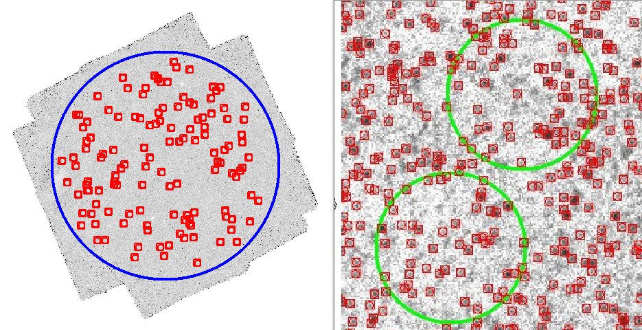
Figure 1: Example of one of the HerMES fields (L6-XMM-LSS-SWIRE) used in our analysis. ($Left$:) HerMES map at 250 $\mu$m; the big circle has radius of 7,800 arcsecs (see Table 1) and encloses the region of the map selected for our analysis, whilst the small squares indicate the position of clusters cataloged by Wen et al. (2012). ($Right$:) A section of the map in which the two large circles indicate the position of two of the Wen et al. clusters, whilst the small symbols indicate the position of sources detected in that map. See the electronic edition of the journal for a color version of this figure.

Fig. 1 presents an example of one of the HerMES maps (L6-XMM-LSS-SWIRE at 250 $\mu$m) used in our analysis. It is shown (left panel) the map and the positions of the clusters detected in the Wen et al. catalog; the panel on the right shows a zoom of the map, with two circles of 5 arcmin radius centered in the position of two clusters, and the sources detected in the HerMES catalog.

3 Analysis and results

3.1 Total emission

Through the line of sight of a given cluster, the HerMES maps contain the contribution from diffuse and point source emissions in the Milky Way, sources (galaxies) members of the clusters, field foreground and background galaxies, any other hypothetical component on superclusters scales, and the possible emission from ICM. To separate the emission of the clusters from the rest of contributors, we follow a statistical approach in which the flux in the angular region projected through each cluster is computed in clustercentric coordinates, and therefore by stacking the emission from many clusters, gradients or spatial irregularities from the rest of contributors (that obviously are uncorrelated with the position of the clusters) are largely filtered out. So, these contaminants can be considered as a spatially uniform background, and subtracted by measuring them in a region far enough from the central position of the cluster. The procedure also smooths any possible spatial asymmetries or irregularities in the emission profile of the clusters, and then in the stacked maps we can ignore any angular dependence and consider only the radial profiles.

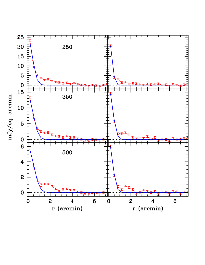
Figure 2: $(Left:)$ Mean radial profiles of the cluster emission for the 250 ($top$), 350 ($middle$) and 500 $\mu$m ($bottom$) channels. $(Right:)$ Mean emission from the sources detected in each of these channels. The solid lines in each panel correspond to gaussian fits in an inner radius of 1 arcmin.

Figure 2 (left) shows the radial profiles of the average flux per cluster obtained by stacking the signal in the 250, 350 and 500 $\mu$m channels for the whole 327 clusters in our sample. The emissions from the clusters are clearly detected in each channel, have a maximum in the center, and show clear declining radial dependences up to $\sim 3-5$ arcmin from the center, whilst from 5 arcmin onwards remain nearly flat. The contribution from contaminants (any other signal apart from the clusters) can be estimated and subtracted by averaging the signal at distances $5-10$ arcmin from the center of the clusters. The signal obtained after such subtraction is our best estimation for the mean emission of the clusters in the whole sample. Although considering larger radius would prevent for removing possible contribution from outskirts of the clusters, in practice the larger area considered and the comparatively low fluxes would largely increase the uncertainty in these estimations.

The spatial profiles of the signals are the result of the convolution of the PSFs of the HERSCHEL maps with the angular extension of the clusters. Gaussian fits to the inner part ($<1$ arcmin) of the radial profiles (solid lines in Figure 2) give FWHMs of 56, 65 and 72 arcsecs for the channels at 250, 350 and 500 $\mu$m respectively. These values are clearly larger than the corresponding instrumental resolutions, and then indicate that the clusters are resolved in the maps. The mean redshift of the sample is 0.37, which corresponds to an angular scale $\sim 5$ Kpc arcsec^-1, and then radius in the range $1-5$ arcmin correspond to linear scales of $0.3-1.5$ Mpc. Table 2 (lines labelled $Total$) shows the integrated fluxes within such range of radius. The signal is higher in the high frequency channel, as it is expected for dust with properties similar to the Milky Way. Some additional uncertainty on the estimation of the total flux results from the bumps in the radial profile centered at $\sim 2-4$ arcmin; these produce a considerable increase of the integrated fluxes from radius 2 to 4 arcmin. These bumps interrupt the decline of the profile with radius, and could be the result of the contribution of a set of clusters with particularly extended profiles, or alternatively the result of fluctuations in the background.

3.2 Separation of the contribution from galaxies and from ICM

Obvious upper limits for any of the two components (galaxies and ICM) are given by the total emission of the clusters in each channel. However, the sensitivity and spatial resolution of HerMES allows partially separate and put tighter constraints on the relative contribution of both components. To do that, we checked if some of the member galaxies of the clusters can be detected in the HerMES maps. Instead of building our own catalog of sources from the maps, we have used those released by the HerMES group; in particular, those obtained using the StarFinder program. Following Wang et al. (2014) that program is particularly useful deblending and identifying faint sources in crowded fields as by construction galaxy clusters are. In general, we do not have information about the redshift of those sources and then it is not possible to assess if a source projected along the line of sight of a given cluster is a member or not of such cluster. Therefore, as it has been done for the maps, we used a statistical approach stacking and averaging the contribution of such sources in clustercentric coordinates. After subtracting a constant background estimated from the emission within radius $5-10$ arcmin from the cluster centers, we have obtained the radial profiles presented in the right panels of Fig. 2. These profiles indicate that some of the sources detected are members of the clusters, and by comparing with the profiles of the total emission, that an important fraction of the emission originated in the cluster comes from these bright discrete sources (galaxies).

Two estimations of the total flux from a direct integration of the profiles are presented in Table 2 (lines labelled $Galaxies$). The FWHMs of gaussian fits to the inner parts $(>1$ arcmin) of the radial profiles are 38, 51 and 49 arcsecs at 250, 350 and 500 $\mu$m respectively. These fluxes contain only the contribution from bright galaxies in the clusters (those bright enough to have been detected and cataloged), so they can be considered as lower limits to the total contribution from galaxies within the clusters. The radial profiles of the fluxes due to the cataloged sources are narrower than the corresponding profiles obtained from the maps. This could be indicative for the presence of some ICM contribution in the outskirts of the cluster or merely a consequence of segregation of galaxies, i. e. prevalence of low luminosity, and then uncataloged sources, in the external regions of the clusters.

The contribution from the ICM can be constrained subtracting from the total emission of the cluster the part that is originated in galaxies. To do that we follow two different estimations (named A and B respectively). Both provide upper limits on the possible emission of the ICM because both estimations include the contribution of sources with fluxes below the sensitivity of the catalog. To subtract the contribution of such sources it would be needed to assumme specific parameters for the luminosity function of galaxies and how they evolve with redshift. This will be considered in a future paper (Gutiérrez et al. in preparation).

Estimation A: An upper limit on the contribution by the ICM is obtained by subtracting from the total emission of the cluster (line $Total$ in Table 2) the contribution of galaxies (line $Galaxies$ in Table 2). The results are also quoted in that table (line $ICM-A$).

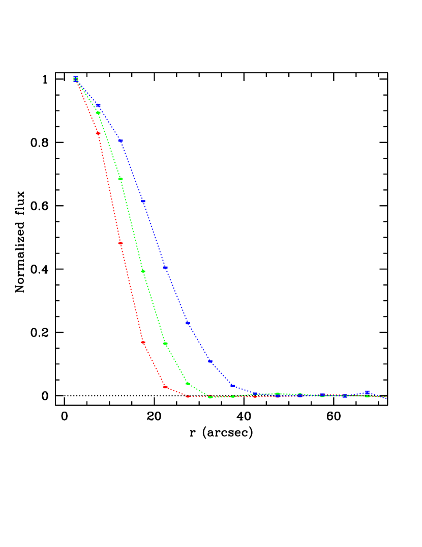
Figure 3: Normalized fluxes of pixels as a a function to the projected distance to the nearest source for the channels at 250 ($red$), 350 ($green$) and 500 $\mu$m ($blue$).

Estimation B: Upper limits on ICM fluxes are estimated by stacking and averaging the fluxes only in those pixels of the maps that are projected far enough from any source in the catalog. We estimate which is the threshold in distance by computing the mean flux of pixels in the maps as a function of the distance to a given source. Figure 3 presents the normalized radial profiles of the fluxes in pixels within distances of 5 arcmin of any cluster, as a function of the projected distance to the nearest source in the HerMES catalogs. These profiles are characterized by FWHMs of 24.2, 31.4 and 41.7 arcsecs for the maps at 250, 350 and 500 $\mu$m respectively. These values are significantly larger than the corresponding instrumental resolutions. For instance, from the instrumental resolution and the radial profile shown in Fig. 3 for the 250 $\mu$m channel, we obtain a FWHM of 16.6 arcsecs as a rough estimation of the mean extension of the sources. In the unrealistic case of all the galaxies being at the mean redshift of the sample of clusters ($\sim 0.37$), that angular extension would correspond to a gaussian profile with $\sigma=35$ Kpc. This is a very crude and biased estimation, because for a given luminosity and radial profile, galaxies at lower redshift will contribute more to the flux, and in practice galaxies spread over a broad distribution of luminosities and profiles which evolve with redshift. Based on the profiles shown in Fig. 3, we defined as regions free of the contribution of bright sources, and therefore suitable to properly constrain the emission of ICM, those lying at distances $>30.8$, $>40.1$ and $>53.2$ arcsecs for the channels at 250, 350 and 500 $\mu$m respectively, from any of the galaxies detected in the HerMES catalogs.

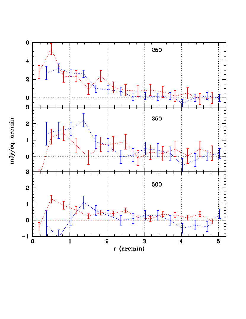
Figure 4: Two diferent estimations (A in $red$ and B in $blue$, see main text for details) of the radial profiles for the 250 ($top$), 350 ($middle$) and 500 $\mu$m ($bottom$) channels of the emission of the clusters after subtracting the contribution of sources bright enough to be detected individually. The results for estimation B ($blue$ lines) have been slightly shifted to the right for visual purposes.

Fig. 4 shows the radial profiles obtained using the A ($red$) and B ($blue$) estimators for the channels at 250, 350 and 500 $\mu$m. Both radial profiles agree quite well apart from the inner part where the noise is higher (the number of pixels used in the estimatios is small), and the angular extension of the sources could have some impact on such estimations. These integrated fluxes within radius $1-5$ arcmin are presented in Table 2 under the lines $ICM-A$ and $ICM-B$ respectively. In general, estimations following $ICM-B$ tend to be somewhat tighter. These fluxes represent estimations of the maximum signal due to ICM, so through the rest of the paper we will follow a conservative approach considering the constraints on the ICM obtained with estimator $A$. From the results obtained within 5 arcmin using that estimator, the 95% upper limits on the ICM surface emission are $1.3\times 10^{-2}$, $0.7\times 10^{-2}$, and $0.5\times 10^{-2}$ MJy str^-1 from the channels at 250, 350 and 500 $\mu$m respectively.

3.3 Dust masses in the ICM

The restriction on the dust mass in the ICM from the above estimation of fluxes requires assumptions of the unknown emissivity (and then chemical composition) of dust particles and on the temperature of the media. These estimations of mass differ by roughly an order of magnitude for dust temperatures within typical ranges (15-25 K) found in studies of extragalactic galaxies (Galametz et al., 2012; Tabatabaei et al., 2014). Adopting a model similar to dust in interstellar regions of the Milky Way (T=20 K and opacities given by the Draine & Lee (1984) silicate-graphite model) we have obtained the results of Table 3. Masses of dust are shown in terms of solar masses and in terms of the total mass of the clusters as estimated by Wen et al. As these estimations come from the fluxes obtained using estimator A and therefore contain also the contribution of faint galaxies, they must be considered as upper limits of dust mass in the ICM. Using the more restrictive limits found using the channel at 350 $\mu$m, the mean ICM mass per cluster within 3 arcmin is $<10^{9}\,M_{\odot}$ or $9.5\times 10^{-6}\,M_{cluster}$ (95% C. L.). The corresponding limits on the projected surface densities are $1.3\times 10^{7}\,M_{\odot}\,arcmin^{-2}$ or $1.2\times 10^{-7}\,M_{cluster}\,arcmin^{-2}$.

The constraints presented here, imply that the gas to mass ratio in ICM is several orders of magnitude smaller than in the Milky Way (Draine, 2003). For instance, taking the limits obtained in the inner 5 arcmin, this defficiency corresponds to $\sim 1.2\times 10^{-3}$ which could be at least partly the result of the relative short living time of dust in the ICM.

3.4 Extinction of background objects

We have estimated upper limits on the visual extinction produced by ICM following a similar approach than in Paper I, i. e. scaling the extinction ($A_{V,MW}=8.6\times 10^{-5}$ mag) and luminosity ($L_{BOL,MW}=2.6\times 10^{43}$ erg s^-1) of the Milky Way (Davies et al., 1997). Considering a model of dust with temperature 20 K and emissivity 2, we have,

$$L_{BOL}=\int_{0}^{\infty}L_{\nu}d\nu=\int_{0}^{\infty}L_{0}\nu^{2}B(\nu,T=20K)d\nu=9.44\times 10^{17}L_{0}\,\Rightarrow L_{0,MW}=2.75\times 10^{18}\,W$$

and for the clusters,

$$L_{\nu_{rest}}=4\pi d_{l}^{2}\frac{F_{\nu}}{1+\bar{z}}=L_{0}\nu^{2}$$

where $L_{\nu_{rest}}=8.89\times 10^{24}$, $7.39\times 10^{24}$ and $3.99\times 10^{24}\,W/Hz$ are the luminosities per unit of rest frequency for the 250, 350 and 500 $\mu$m channels respectively, $\bar{d}_{l}$ and $\bar{z}$ are the mean luminosity distances and redshifts of the clusters, whilst $F_{\nu}$ are the limits of the fluxes for ICM emission as quoted in Table 3. For the 327 clusters considered in this work, $\bar{d}_{L}=2,228$ Mpc and $\bar{z}=0.371$. The upper limits on the extinction within radius from 1 to 5 arcmin derived from each of the channels are shown in Table 4. These values correspond to maximum values assuming the unrealistic case of negligible contribution from faint sources. In any case, they are probably the best limits found for the extinction through clusters.

4 Estimating dependences with redshift and mass

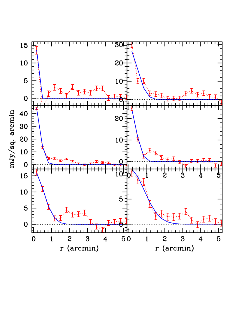
Figure 5: Radial profiles of the mean fluxes in the 250 $\mu$m channel for clusters in two ranges of masses ($left:$ $<10^{14}$ and $right:$ $>10^{14}\,M_{\odot}$) and three of redshifts ($top:$ $<0.24$, $middle:$ $0.24-0.42$ and $bottom:$ $>0.42$). The solid lines correspond to gaussian fits to such profiles.

The range in redshift and mass spanned by the sample of clusters used allows to study the possible evolution of fluxes, masses and extinctions as functions of both parameters, redshift and mass. That was done by separating the clusters according to three ranges in redshift $<0.24$, $0.24-0.42$ and $>0.42$, and two in mass ($<10^{14}$ and $>10^{14}M_{\odot}$) respectively. We repeat for each of the bins the procedure of stacking, separation of components, and estimation of physical magnitudes carried out for the whole sample. The radial profiles of the mean fluxes for each of the division in redshift and mass are presented in Fig. 5. Although the comparatively low number of clusters considered in each bin respect to the whole sample obviously increases the noise on the estimation of fluxes, these are clearly detected in each subgroup of redshift and mass. The gaussian fits to these profiles, shown as solid lines in the figure, are able to reproduce reasonably well the inner 1 arcmin in all cases apart from the bin that corresponds to $<10^{14}M_{\odot}$ and redshift $<0.24$. The radial profiles show that clusters tend to be more extended with redshift. This effect is not present in the estimations of sizes from the distribution of galaxies in the optical as was done by Wen et al., and could be indicative of star formation in the outskirts of high redshift clusters by galaxies in the process of being accreted.

4.1 Extinction of background objects

Table 5 presents the upper limits obtained on the visual extinction of background objects for the three bins in redshift and two in mass of clusters considered. The columns are the number of clusters in each bin, the mean redshift and mass, and the 95% upper limit on the visual extinction within a radius of 5 arcmin obtained from the 250, 350 and 500 $\mu$m channels respectively. The three channels independently allow to put constraints at levels below $\sim 1$ milimag for any of the subdivisions in redshift and mass considered.

4.2 Evolution of the infrared luminosity

Studying the possible evolution of luminosity with redshift and/or mass could give information about the general processes ruling the accretion of galaxies by clusters, and the internal mechanisms that could affect the evolution of galaxies and the star formation processes. Through this section, we consider the whole luminosity of the cluster ignoring the possible contribution of the ICM. The analysis below implicitly assummes that physical conditions and evolution of dust in ICM and galaxies are similar. For this analysis, we considered the emission within a 5 arcmin radius. Instead of integrating the profiles of each bin in the three channels, we have chosen the channel 250 $\mu$m as reference, and estimated the fluxes in the other two channels by scaling the integrated fluxes at 250 $\mu$m according to the relative signals in the central bins. We estimated the corresponding luminosities per unit of rest framed frequency, $L_{\nu_{rest}}$, considering the luminosity distance $d_{l}$ at the mean redshift of each bin, and correcting to a rest framed system, i e. $L_{\nu_{rest}}=4\pi d_{l}^{2}F_{\nu}/(1+z)$, where $\nu$ is the observed frequency of each of the three channels, and $\nu_{rest}=\nu(1+z)$. The frequencies observed for a given channel correspond to different rest framed frequencies according to the redshifts of the clusters, therefore, in order to do a proper comparison of luminosities, it is necessary to estimate the luminosities at a particular rest framed frequency or to estimate the total far infrared luminosity ($L_{FIR}$) by assuming a model for the emission of the dust.

A model in which the emission of dust corresponds to a modified black body with a temperature $T$ and an emissivity $\beta$, i. e. $L=\int L_{\nu}d\nu=K\int\nu^{\beta}B_{\nu}(T)d\nu$ gives an adequate description of most of the dust emission at $\lambda\geq 50\,\mu m$. Leaving unconstrained the three parameters ($K,\,\beta$ and $T$), reasonable fits from the estimated luminosities in the 250, 350 and 500 $\mu$m channels are obtained for values of $T\sim 20-25\,K$ and $\beta\sim 2$. However, the relatively small spectral range covered by the three channels, the high noise on the estimation of luminosities, and the known degeneracy between temperature and emissivity, make convenient to reduce the number of free parameters. In the analysis presented below, we chose $T=20\,K$ and $\beta=2$. Nevertheless, the estimations of the relative luminosities do not depend much on the exact values of these parameters. Fig. 6 presents the luminosities per unit of frequency for each of the channels obtained for clusters in the ranges of redshift and mass considered, and the best fits (dashed lines) obtained for this model. In general, the model reproduces well the data with predictions within the error bars of the estimated luminosities. The bolometric luminosities obtained for these models are presented in Table 6. These results show a clear dependence of luminosity with redshift whilst the possible dependence on mass, if any, is less conspicuous.

The evolution of luminosity with redshift and mass was modeled according to $L=\Upsilon M^{\alpha_{M}}z^{\alpha_{z}}$, with $\Upsilon$, $\alpha_{M}$ and $\alpha_{z}$ parametrizing the overall normalization, and the possible dependence with mass and redshift respectively. A chi-square fit gives $\Upsilon=1.60\times 10^{44}\,erg\,s^{-1}$, $\alpha_{M}=-0.24$ and $\alpha_{z}=1.47$. Given the number of assumptions and systematic uncertainties associated to this procedure, we have not tried to quote errors in these parameters. The fit is able to reproduce well the data although obviously the relatively low luminosity of the intermediate redshift, high mass bin is somewaht out of the general trend. We have checked that the fluxes measured for this bin in the three channels are clearly lower than those in the low mass bin at the same redshift. It would be interesting to investigate this in the future with more Herschel data, in order to see if some systematics is present in the estimation of fluxes, or the results just show particularities in the evolution of high mass clusters at intermediate redshifts. Excluding that bin from the analysis, the fit notably improves with differences between the data and the fits within $\sim 20\%$. The fit gives $\Upsilon=1.73\times 10^{44}\,erg\,s^{-1}$, $\alpha_{M}=0.36$, and $\alpha_{z}=1.57$. In any case, the strong dependence of the luminosity with redshift is quite robust as it was demonstrated by conducting numerous tests in which we split the data changing the number of bins in redshift and mass. We also repeat the analysis, using the luminosities estimated from the gaussian fits to each of the radial profiles. Using those luminosities we obtain $\Upsilon=1.16\times 10^{44}\,erg\,s^{-1}$, $\alpha_{M}=-0.29$ and $\alpha_{z}=1.48$.

More realistic models of dust emission (Draine & Li, 2007) show that the modified back body models underestimate the dust emission at very long wavelengths ($>1000\,\mu m$) and do not describe the spectral range shortwards than $\sim 50\,\mu m$, in which emission associated to polycyclic aromatic hydrocarbon (PAH) material is the dominant process. This is important in order to estimate $L_{FIR}$, which is used as an estimator of the $SFR$ (Kennicutt, 1998) (see below). The relative emission at short wavelengths depends on the amount of PAHs and on the properties of the radiation field. As representative of these models, we fit the luminosities in each of the 3 x 2 samples in redshift and mass respectively to a Milky Way like model with a fraction of PAHs of 4.6%, and exposed to a single radiation intensity as computed by Draine & Li (2007) (see that paper for full details). Fitting the luminosities from the integrated fluxes within 2 arcmin in the three channels, we obtained the fits presented in Fig. 6 (solid lines). The figure shows that these models reasonably fit the data and predict emission similar to the modified black body model in the range $\sim 50-500\,\mu m$. We are aware of the uncertainties in the estimation of $L_{FIR}$ due to the contribution of dust at wavelengths shorter than $\sim 50\,\mu m$ that are not sampled by the HERSCHEL data, however this uncertainty is mostly systematic and likely affects in a similar way to the six subsamples. Repeating the above analysis with the luminosities estimated from the Draine & Li (2007) model, we obtain $\Upsilon=1.23\times 10^{44}\,erg\,s^{-1}$, $\alpha_{M}=-0.16$, $\alpha_{z}=1.63$, and $\Upsilon=1.73\times 10^{44}\,erg\,s^{-1}$, $\alpha_{M}=-0.33$, $\alpha_{z}=1.53$ for the luminosities obtained integrating directly the radial profiles within a 5 arcmin radius, and from the gaussian fits respectively. To study separately the evolution with redshift for the low and high mass samples, we fit functions $L\sim z^{\alpha_{z}}$ (i. e. $\alpha_{M}=0$) for the low and high mass subsamples and obtained $\alpha_{z}=1.93$ and $1.35$ respectively.

To check how the parameters $\alpha_{M}$ and $\alpha_{z}$ depend on the model used to parametrize the cluster luminosities, we also simply fit a straight line to the luminosities derived for each of the three channels and subsamples of redshift and mass, and take the interpolate value at a given frequency. Using the luminosities at $\nu_{rest}=1250\,GHz$, we obtain $\alpha_{M}=-0.1$ and $\alpha_{z}=1.5$.

The dependence of luminosity with redshift and mass translates directly into SFR; using Kennicutt (1998) calibration, i. e. $SFR\,(M_{\odot}\,yr^{-1})=4.5\times 10^{-44}\,erg\,s^{-1}L_{FIR}$ (see Kennicutt & Evans (12) for a discussion and comparison between different SFR estimators), our results show a strong declining of $SFR$ for clusters in both ranges of masses ($<10^{14}$ and $>10^{14}$ M_⊙) by nearly an order of magnitude in a period of $\sim 6$ Gyr. This estimation ignores the contribution to luminosity from AGNs; however we implicitly assume a coevolution of black holes and $SFR$ in, at least, the last 10 Gyr,see e. g. Shankar (2009) and the evidence summarized in Heckman & Best (2014). So, ignoring AGNs contribution, the absolute calibration of SFR could be affected but in the same way at any redshift. The little dependence of $L_{FIR}$ with mass indicates a specific star formation rate, $SFR/M$ anticorrelated with mass (excluding the intermediate redshift high mass bin, we obtain $SFR/M\sim M^{-0.64}$). This anticorrelation support, as many other authors have shown in the past (e. g. (Balogh et al., 1998) that the declining of $SFR$ in clusters with time is not merely a consequence of accretion of galaxies with less $SFR$ at a given cosmic time, but instead it is also a consequence of internal processes in the clusters.

5 Comparison with previous studies

A similar approach to our method B was used by Kitayama et al. (2009) and applied to ISO data at 70 and 160 $\mu$m in the Coma cluster. These authors obtained $A_{V}<0.011$ mag within the central 100 Kpc of the cluster. It is not possible to conduct a direct comparison between their results and our findings (Tables 4 and 5) due to the use of different samples, and the slightly different way to estimate the extinctions. However, both results point out to a very small extinction within the central parts of the clusters, being our upper limits an order of magnitude tighter. We also improve by roughly and order of magnitude the constraints obtained by Muller et al. (2008). Our results are also compatible and improve the limits ($E(B-V)<8\times 10{-3}$ mags on 1 Mpc scales) found by the Bovy et al. (2008). The differential extinction found in the analysis by Chelouche et al. (2007) from the differential reddening of galaxies in the background of clusters found in the analysis by Chelouche et al. (2007) (see their Fig. 3) seems to occur at clustercentric distances $>2R_{200}$. As was noted in Paper I, our results are difficult to fit with those by Mc Gee et al. (2010) who analyzed a sample of low redshift groups and clusters, and found extinctions $\sim 10^{-2}$ mag on scales $\sim 10$ Mpc. At the mean redshift of our sample, 5 arcmin subtends $\sim 1.5$ Mpc, and assumming a linear decrease of dust attenuation with clustercentric distance, the results by such authors (see their Fig. 4) would correspond to $A_{v}\sim 0.002$ mag. This is still about one order of magnitude smaller that the typical values quoted in our Table 4. Although Fig. 4 by McGee et al. seems indicate a shallower behaviour of the differential extinction in the very inner parts of the cluster, it is difficult a strong assesment on this due to the low angular/spatial resolution of such results.

Comparing with the results presented in Paper I, the use of three frequencies, and the best sensitivity and spatial resolution of the HerMES maps with respect to IRAS, largely compensates the smaller spatial coverage (and then the numbers of clusters used) in the present work. Considering as representative of the results obtained in Paper I, the 95% upper limit of $E(g-i)=3.6$ milimags found within the central 1 Mpc, the constraints presented here (Table 4) improve that by roughly an order of magnitude.

Our results qualitative agree with many previous works that have estimated the infrared luminosity up to redshift $\sim 1$. They show a strong increase of luminosity, and therefore $SFR$, with redshift, in the field, in groups and in clusters, being unclear whether or not the evolution is similar in any of these environments. Although it is difficult to establish rigurous comparison due to the different methods, samples, and redshifts covered, the evolution found in the present work is stronger than the dependence $\sim(1+z)^{3.9}$ found by Le Floc’h et al. (2005) in field galaxies up to $\sim 1$ found by Spitzer Werner et al. (2004) in the Chandra Deep Field South. Other authors, (Dye et al., 2010) have found in field galaxies a stronger dependence in luminosity with redshift $\sim(1+z)^{7}$ that agrees better with our results.

We qualitatively agree also with the findings by Guo et al. (2014) and Popesso et al. (2012) who found increase in luminosity with redshift in groups and clusters with masses in the ranges $(10^{12}-10^{14})h^{-1}M_{\odot}$ and $(10^{13}-10^{15})M_{\odot}$ respectively, and with the strong evolution in luminosity found also by Bai et al. (2009) comparing local and high redshift ($\sim 0.8$) clusters. Clements et al. (2014) by analyzing Herschel-SPIRE maps and the Planck Early Release Compact sources catalog (Planck collaboration, 2011) identified and estimated the luminosities and $SFRs$ of four candidates to be clusters of galaxies at redshifts $\sim 1-2$. Although these sources correspond likely to very extreme cases that are not representative of the average values found in the analysis of Wen et al clusters, their own existence points towards an increase in luminosity, and therefore in $SFR$, very strong at least up to redshift $\sim 2$.

6 Conclusions

Constraints on the ICM emission at 250, 350 and 500 $\mu$m have been obtained using a sample of 327 clusters of galaxies spanning ranges of 0.05-0.7 in redshift and $>4\times 10^{13}M_{\odot}$ in mass, and maps and catalogs of sources at 250, 350 and 500 $\mu$m from the HERSCHEL HerMES project. The main results are:

1. Subtracting from the whole emission of the cluster the contribution of identified sources, it has been estimated 95% upper limits on the ICM emission per cluster of 86.6, 48.2 and 30.9 mJy in the maps at 250, 350 and 500 $\mu$m respectively within a 5 arcmin radius centered in each cluster. These correspond to surface emission of $1.3\times 10^{-2}$, $0.7\times 10^{-2}$, and $0.5\times 10^{-2}$ MJy str^-1 respectively.

2. Assuming for the intracluster dust typical values found within the Milky Way (a temperature of 20 K, and an emissivity $\beta=2$), we have obtained strong upper limits on the visual extinction of background objects due to the ICM. From the fluxes at 250, 350 and 500 $\mu$m these restrictions are respectively $A_{V}(95\%\,C.L.)<$ 0.4, 0.4 and 0.6 milimags within projected distance of 5 arcmin from the cluster centers. Separating the clusters in 3 x 2 bins in redshift and mass respectively, the constraints on the extinctions are of the order of 1 milimag in any of the ranges in redshift and mass considered.

3. Tight upper limits are also obtained on the dust mass in the ICM; for instance using the data at 350 $\mu$m we set a 95% upper limit of $<10^{9}M_{\odot}$ within a projected 5 arcmin radius circle centered in the clusters. This corresponds to a fraction of the total mass of the clusters of $9.5\times 10^{-6}$.

4. From the results obtained in the three channels, we have estimated $L_{FIR}$ and its dependence of the far infrared luminosity with redshift and mass. Although there are many assumptions and the estimations are slightly model dependent, the overall results show a clear and strong dependence with redshift $\sim z^{1.5}$, whilst the dependence with mass is not so obvious indicating an anticorrelation of $L_{FIR}/M$ with the mass of the cluster. Using the linear relation between $L_{FIR}$ and $SFR$, the results indicate a declining by roughly an order of magnitude in $SFR$ in a period of $\sim 6$ Gyr. The specific $SFR$ is clearly anticorrelated with mass; this indicates that internal mechanisms play a role on this quenching of $SFR$.

Figure 6: Luminosities per unit of frequency obtained for clusters in the three ranges of redshift (from top to bottom: $0.05-0.24$, $0.24-0.42$ and $>0.42$), and two of mass (left: $<10^{14}M_{\odot}$ and right $>10^{14}M_{\odot}$). The units of the vertical axis are $erg\,s^{-1}Hz^{-1}/10^{31}$ whilst the horizontal axis corresponds to rest framed frequencies. Dashed and dotted lines correspond to the best fits for a model $\sim\nu^{2}B_{\nu}(T=20K)$ and for a Draine & Li (2007) model respectively (see main text for details).

Table 1: HerMES fields used in this work

Field	RA (hh:mm:ss)	Dec. (o ${}^{{}^{\prime}}$ ${}^{{}^{\prime\prime}})$	Radius (arcsec)	Clusters	Sources
L5-Lockman-SWIRE	10 46 47.61	+58 04 38.0	6000	72	2467
L5-Bootes-HerMES	14 32 37.03	+34 10 17.6	5400	80	3827
L5-ELAIS-N1-HerMES	16 10 11.02	+54 19 30.3	3000	16	826
L6-XMM-LSS-SWIRE	2 20 35.99	-4 31 43.4	7800	129	5177
L6-FLS	17 16 12.74	+59 23 01.7	4200	30	1272

Table 2: Integrated fluxes of the average emission of 327 clusters.

$Channel$	$Radius$	$Total$	$Galaxies$	$ICM-A$	$ICM-B$
	$(arcmin)$	$(mJy)$
250	1	$27.3\pm 0.9$	$16.8\pm 1.0$	$10.5\pm 1.3$	$9.0\pm 0.9$
	2	$55.8\pm 2.5$	$27.7\pm 2.7$	$28.1\pm 3.7$	$21.9\pm 2.4$
	3	$81.8\pm 4.5$	$40.0\pm 5.0$	$41.8\pm 6.7$	$26.8\pm 4.3$
	4	$101.6\pm 6.9$	$47.4\pm 7.7$	$54.2\pm 10.3$	$24.4\pm 6.5$
	5	$118.2\pm 9.7$	$60.4\pm 10.7$	$57.8\pm 14.4$	$26.7\pm 9.0$
350	1	$17.7\pm 0.6$	$14.4\pm 0.7$	$3.3\pm 0.9$	$5.1\pm 0.9$
	2	$38.7\pm 1.6$	$31.1\pm 1.9$	$7.6\pm 2.5$	$16.0\pm 2.3$
	3	$57.0\pm 2.9$	$41.8\pm 3.5$	$15.2\pm 4.5$	$19.3\pm 4.0$
	4	$73.7\pm 4.5$	$51.6\pm 5.4$	$22.1\pm 7.0$	$19.5\pm 6.0$
	5	$82.3\pm 6.2$	$53.5\pm 7.5$	$28.8\pm 9.7$	$20.0\pm 8.3$
500	1	$8.6\pm 0.3$	$5.8\pm 0.3$	$2.8\pm 0.4$	$-1.0\pm 1.0$
	2	$18.7\pm 0.9$	$11.8\pm 0.7$	$6.9\pm 1.1$	$4.6\pm 2.1$
	3	$26.0\pm 1.6$	$13.3\pm 1.3$	$12.7\pm 2.1$	$6.4\pm 3.4$
	4	$34.6\pm 2.4$	$16.2\pm 2.0$	$18.4\pm 3.1$	$4.3\pm 5.0$
	5	$38.0\pm 3.3$	$15.7\pm 2.8$	$22.3\pm 4.3$	$1.2\pm 6.7$

Table 3: Upper limits on the dust mass in the ICM.

$Channel$	$Radius$	$M_{dust}$
	$(arcmin)$	$10^{7}M_{\odot}$	$10^{-7}M_{cluster}$
250	1	$13.8\pm 1.7$	$12.5\pm 1.6$
	2	$36.9\pm 4.9$	$33.5\pm 4.4$
	3	$54.8\pm 8.8$	$49.9\pm 8.0$
	4	$71.1\pm 13.5$	$64.7\pm 12.3$
	5	$75.8\pm 18.9$	$69.0\pm 17.2$
350	1	$7.2\pm 2.0$	$6.5\pm 1.8$
	2	$16.5\pm 5.4$	$15.0\pm 4.9$
	3	$33.0\pm 9.8$	$30.0\pm 8.9$
	4	$48.0\pm 15.2$	$43.7\pm 13.8$
	5	$62.5\pm 21.1$	$56.9\pm 19.2$
500	1	$14.2\pm 2.0$	$12.9\pm 1.8$
	2	$34.9\pm 5.6$	$31.8\pm 5.1$
	3	$64.3\pm 10.6$	$58.5\pm 9.7$
	4	$93.2\pm 15.7$	$84.7\pm 14.3$
	5	$112.9\pm 21.8$	$102.7\pm 19.8$

Table 4: Maximum visual extinctions ($A_{V}$) for objects in the background of clusters derived from the constraints in the ICM flux at 250, 350 and 500 $\mu$m.

Channel	$A_{V}$ (milimag)
	$1^{{}^{\prime}}$	$2^{{}^{\prime}}$	$3^{{}^{\prime}}$	$4^{{}^{\prime}}$	$5^{{}^{\prime}}$
250	1.7	1.1	0.8	0.6	0.4
350	1.1	0.7	0.6	0.5	0.4
500	0.7	0.9	0.7	0.6	0.6

Table 5: Extinctions of background objects as a function of redshift and mass of the cluster. The three last columns correspond to the 95% upper limits obtained for $A_{V}$ within a 5 arcmin radius from the center of the clusters, using the results from the 250, 350 and 500 $\mu$m channels respectively.

Clusters	Redshift	(Mass/$10^{14}M_{\odot}$)	$A_{V}$ (milimag)
41	0.189	0.74	0.1	0.3	0.6
35	0.174	1.59	0.2	0.3	0.2
73	0.335	0.74	0.5	0.6	0.9
52	0.334	1.55	0.2	0.1	0.1
72	0.528	0.75	1.0	0.4	1.1
54	0.513	1.56	0.4	0.5	0.7

Table 6: Luminosities in three ranges of redshift ($<0.24$; $0.24-0.42$ and $>0.42$) and two of mass ($<10^{14}$ and $>10^{14}M_{\odot}$).

Range in mass		Range in redshift
		0.06-0.24	0.24-0.42	0.42-0.71
$<1$	${\it 1.}$	0.185	0.333	0.527
	${\it 2.}$	0.74	0.74	0.75
	${\it 3.}$	41	73	72
	${\it 4.}$	2.9	9.2	20.1
$>1$	${\it 1.}$	0.173	0.338	0.517
	${\it 2.}$	1.59	1.55	1.56
	${\it 3.}$	35	52	54
	${\it 4.}$	4.7	2.9	18.8

References

- Bai et al. (2007) Bai, L., Rieke, G. H., & Rieke, M. J. 2007, ApJ, 668, L5
- Bai et al. (2009) Bai, L., Rieke, G. H., Rieke, M. J., Christlein, D., & Zabludoff, A. I. 2009, ApJS, 182, 543
- Bennett et al. (1992) Bennett, C. L. et al. 1992, ApJ, 369, L7
- Balogh et al. (1998) Balogh, M. L., Schade, D., Morris, S. L., et al. 1998, ApJ, 504, L75
- Bovy et al. (2008) Bovy, J., Hogg, D. W., & Moustakas, J. 2008, ApJ, 688, 198
- Chelouche et al. (2007) Chelouche, D., Koester, B. P., & Bowen, D. V. 2007, ApJ, 671, L97
- Clements et al. (2014) Clements, D. L. et al. 2014, MNRAS, 439, 1193
- Davies et al. (1997) Davies, J. I. et al. 1997, MNRAS, 288, 679
- Draine (2003) Draine, B. T. 2003, ARA&A, 41, 241
- Draine & Lee (1984) Draine, B. T., & Lee, H. M. 1984, ApJ, 285, 89
- Draine & Li (2007) Draine, B. T., & Li, A., ApJ, 2007, 657, 810
- Dye et al. (2010) Dye, S. 2010, A&A 518, 10
- Galametz et al. (2012) Galametz, M. et al. 2012,, MNRAS, 425, 763
- Giard et al. (2008) Giard, M.,Montier, L., Pointecouteau, E., & Simmat, E. 2008, A&A, 490, 547
- Griffin et al. (2010) Griffin, M. J. et al. 2010, A&A, 518, L3
- Guo et al. (2014) Guo, Q. et al. 2014, MNRAS, 442, 2253
- Gutiérrez & López-Corredoira (2014) Gutiérrez, C. M. & López-Corredoira, M. 2014, A&A, 571, 66
- Heckman & Best (2014) Heckman, T. M., & Best, P. N. 2014, ARA&A, 52, 589
- Kennicutt (1998) Kennicutt, R. C. Jr. 1998, ARAA, 36, 189
- Kennicutt & Evans (12) Kennicutt, R. C. Jr., & Evans, N. J. II 2012, ARA&A, 50, 531
- Kitayama et al. (2009) Kitayama, T., et al. 2009, ApJ, 695, 1191
- Le Floc’h et al. (2005) Le Floc’h, E. et al. 2005 ApJ, 632, 169
- Levenson et al. (2010) Levenson, L. et al. 2010, MNRAS, 409, 83
- Mc Gee et al. (2010) McGee, S. L., & Balogh, M. L. 2010, MNRAS, 405, 2069
- Montier & Giard (2005) Montier, L. A., & Giard, M. 2005, A&A, 439, 35
- Muller et al. (2008) Muller, S. et al. 2008, ApJ, 680, 975
- Nollenberg et al. (2003) Nollenberg, J. G., Williams, L. L. R., & Maddox, S. J. 2003 ApJ, 125, 2927
- Oliver et al. (2012) Oliver, S. J. et al. 2012, MNRAS, 424, 1614
- Pilbratt et al. (2010) Pilbratt, G. L. et al. 2010, A&A, 518, L1
- Planck collaboration (2011) Planck Collaboration 2011, A&A, 536, 7
- Popesso et al. (2012) Popesso, P. et al. 2012, A&A, 537, A58
- Roseboom et al. (2010) Roseboom, I. G. et al. 2010, MNRAS, 409, 48
- Shankar (2009) Shankar, F. 2009, NewAR, 53, 57
- Schlegel et al. (1998) Schlegel, D. J. Finkbeiner, D. P, & Davis, M. 1998, ApJ, 500, 525
- Stickel et al. (2002) Stickel, M., Klaas, U., Lemke, D., & Mattila, K. 2002, A&A, 383, 367
- Smith et al. (2012) Smith, A. J. et al. 2012, MNRAS, 419, 377
- Tabatabaei et al. (2014) Tabatabaei, F. S. et al. 2014, A&A, 561, A95
- Wang et al. (2014) Wang, L. et al. 2014, MNRAS, 444, 2870
- Wen et al. (2012) Wen, Z. L., Han, J. L., & Liu, F. S. 2012, ApJS, 199, 34
- Werner et al. (2004) Werner, M. W. et al. 2004, ApJS, 154,1
- Wheelock et al. (1993) Whhelock, S. et al. 1993, ISSA, Explanatory Supplement, Technical Report (Pasadena: IPAC)
- Zwicky (1962) Zwicky, F. 1962, in, Problems of Extragalactic research, ed. G. C. McVittie (NY: Macmillan), 149