iint \savesymboliiint \restoresymbolTXFiint \restoresymbolTXFiiint
The Precise and Powerful Chaos of the 5:2 Mean Motion Resonance with Jupiter
Abstract
This work reexamines the dynamics of the 5:2 mean motion resonance with Jupiter located in the Outer Belt at AU. First, we compute dynamical maps revealing the precise structure of chaos inside the resonance. Being interested to verify the chaotic structures as sources of natural transportation routes, we additionally integrate 1000 massless particles initially placed along them and follow their orbital histories up to 5 Myr. As many as 99.5% of our test particles became Near-Earth Objects, 23.4% migrated to semi-major axis below 1 AU and more than 57% entered the Hill sphere of Earth. We have also observed a borderline defined by the AU perihelion distance along which particles escape from the Solar System.
keywords:
minor planets, asteroids, general – meteorites, meteors, meteoroids – chaos – diffusion1 Introduction
Some of the most important resonances in our Solar System are those capable of driving bodies from different parts of the Main Belt down to the neighborhood of Earth, to the so called Near Earth Object (NEO) region. By convention, NEO region is defined for perihelion distances smaller than AU and aphelion distances larger than AU (Rabinowitz et al, 1994).
A generally accepted dynamical scenario played by those ’important’ resonances evolves according to the following principle: the asteroid is slowly driven into the resonance by the Yarkovsky effect (Vokrouhlický and Farinella, 2000) or becomes directly injected into it by some collisional event. The semi-major axis of the resonant asteroid stays almost constant, while its eccentricity slowly increases up to planet crossing values (Wetherill and Williams, 1979; Wisdom, 1983), opening possibilities for close encounters. Depending on its proximity to the planet and mass, the asteroid may or may not survive the close encounter. We do not go into detailed description of all the possible close encounter outcomes, but in general, the small body continues its journey through the phase-space governed by the subsequent close encounters or captures into other resonance/s, until it collides with a planet or the Sun, becomes ejected to hyperbolic orbits or drives out of the Solar system.
First systematic numerical studies on the most prominent Main Belt resonances performed by Gladman et al (1997), showed that the evolutionary processes driving bodies to the NEO region unfold mostly due to three Main Belt resonances: the secular resonance located at AU, 3:1 and 5:2 mean motion resonances (MMRs) with Jupiter, at AU and AU respectively. The 5:2 resonance, the subject of our study, was considered as the least efficient in that respect, since most particles placed into that resonance, after approaching Jupiter, were ejected out to hyperbolic orbits. Similar results were obtained in another round of numerical studies by Bottke et al (2002), who claimed that only 8% of the NEO population comes from the outer belt ( AU which includes the region of the 5:2 resonance). Furthermore, de Elía and Brunini (2007) estimated that as many as 94% of NEAs (Near Earth Asteroids) arrived from the Main Belt region inside the 5:2 MMR, confirming that the Outer Belt has a negligible role in the dynamical processes supplying the NEO region.
On the other hand, spectral analysis suggests that a large number of ordinary L chondrite meteorites could have been driven down to Earth from the outer belt in very short delivery times (<1-2 Myr). The main candidate for the asteroidal source of L-chondrite meteorites is the outer belt asteroid family Gefion, whose fragments, after a catastrophic breakup Myr ago, rapidly evolved to Earth-crossing orbits via the nearby 5:2 mean motion resonance with Jupiter (Nesvorný et al, 2009). However, the authors asserted that ’a potential problem with this result should be the low efficiency of meteorite delivery from the Gefion family location’.
Asteroid (3200) Phaethon, the parent body of the Geminids meteor shower, arrived in the NEO region most likely from the asteroid family Pallas (located in the Outer Belt), via its bordering 8:3 or 5:2 MMRs with Jupiter (de Leon et al, 2010). Still, dynamical models in de Leon et al (2010); Bottke et al (2002) showed that less than of the test particles placed into the 5:2 resonance recovered a Phaethon-like orbit. We mention another candidate that most likely arrived from the Outer Belt Koronis family via the 5:2 resonance - one of the largest Potentially Hazardous Asteroids - 2007 PA8 (Sanchez et al, 2015; Nedelcu et al, 2014).
Thus, a growing number of meteorites and NEOs whose spectral type indicates an Outer Belt origin and which have been driven to the NEO region via the 5:2 resonance, does not match well with its low transportation efficiency suggested in dynamical studies.
Let us notice that a common feature in the studies of Bottke et al (2002); Gladman et al (1997); Morbidelli and Gladman (1998); de Elía and Brunini (2007) and de Leon et al (2010) is that unbiased initial data sets were used, with no particular selection from the most unstable parts of the resonance. Moreover, Gladman et al (1997) claimed that the initial location inside the resonance should not have a significant influence on the orbital scenaria.
Here we reexamine the transportation abilities of the 5:2 resonance using the same principle as in the above mentioned studies, with the exception that the test particles are carefully chosen at the most unstable parts of the resonance, whose localization is enabled by the computation of highly precise FLI (Fast Lyapunov Indicator) dynamical maps.
The article is organized as follows. In Section 2 we give a brief definition of the Fast Lyapunov Indicator and in Section 3 we show and describe the FLI maps we have computed using a Solar System model with and without the inner planets. A short description of the way we select the 1000 particles in order to confirm the high transportation abilities of the 5:2 resonance is given in Section 4. The resulting orbits are discussed in Section 5, while the Conclusions are provided in Section 6. In the supplementary data (on-line only) we list the exact initial values of the orbital elements of 1000 rapidly evolving particles and show some additional results on the 5:2 MMR.
2 The Fast Lyapunov Indicator-FLI
The Fast Lyapunov Indicator (Froeschlé et al, 1997b, a) is one of the most efficient chaos detection tools used mainly to produce dynamical maps. In the beginning FLI was used for idealized systems such as symplectic maps or simplified Hamiltonians (Froeschlé et al,, 2000; Lega and Froeschlé, 2003; Froeschlé et al,, 2005; Todorović et al, 2008, 2011), but later FLI was successfully applied in studies of asteroids or planetary systems as well, starting from the close neighborhood of Earth (Daquin et al, 2016; Rosengren, 2015), up to the outer Solar System (Guzzo, 2005, 2006). FLI maps were also produced for the region between Earth and Venus by Bazsó et al (2010), Main Belt maps were computed in Galeş (2012), investigation of the asteroid family Pallas based on FLI maps was performed in Todorović and Novaković (2015) and finally, exoworlds have also been extensively studied by FLI, for example in Pilat-Lohinger et al (2002); Dvorak et al (2003); Sándor (2007); Schwarz (2011). What follows is a brief definition of FLI.
Let us consider a continuous dynamical system defined by a set of differential equations
| (1) |
where is a differentiable function defined on a manifold For a given initial value and its corresponding initial nonzero deviation vector lying in the tangent space of , the Fast Lyapunov Indicator is defined as the logarithm of the norm of the deviation vector at some fixed time , i.e. by the quantity:
| (2) |
In the above definition time plays the role of a parameter, while the supremum is used only to annul some local oscillations that may influence the result.
When it comes to the numerical evaluation of FLI, one has to follow both the orbit and its corresponding deviation vector . Time evolution of is obtained by integrating the equations of motion (1), while the evolution of is released by integrating the so-called variational equations:
where is an operator which maps the tangent space of at point onto the tangent space at point .
If the orbit is regular, the norm of its deviation vector grows linearly over time. For chaotic orbits grows exponentially. Stronger chaos implies its faster increment and hence larger FLI values.
Using FLI basically means that we do not have to wait a long time for the orbit to show its dynamical character through the asymptotic properties of its deviation vectors. The integration time should be short enough just to capture the difference between resonant, nonresonant or chaotic orbits of different strengths.
Moreover, Guzzo and Lega (2014) illustrated that tangent vectors grow faster if the initial condition of the orbit is close to stable-unstable manifolds of the hyperbolic fixed point of a resonance. Such orbits will have small FLI ridges that can be captured only at the beginning of the integration. Therefore, calculation of FLI maps with a careful choice of the computing time allows a clear visualization of the hyperbolic structures inside the resonance, opening up many possibilities for their further investigation.
3 FLI maps of the resonance with Jupiter
The FLI maps of the dynamical structure in the region of the 5:2 mean motion resonance with Jupiter is represented on the two panels composing Fig. 1. The first, above panel, is calculated taking into account the planets in the Solar System, from Venus to Neptune, while Mercury’s mass is added to the mass of the Sun and the corresponding barycentric correction is applied to the initial conditions. The lower, bottom map is computed including only the outer planets: Jupiter, Saturn, Uran and Neptune.
For each of the particles regularly distributed along a grid for we have computed its corresponding FLI for 10 000 years. Inclinations for all the particles are set to (corresponds to the orbital plane of the most massive asteroid Ceres), while the orbital angles are fixed at random values . On the color scale, stable particles with FLIs below 0.9 are red, while the most chaotic ones with are yellow.
All the calculations are made using the ORBIT9 integrator111Available from http://adams.dm.unipi.it/orbfit/ that operates on a symplectic single step method (implicit Runge-Kutta-Gauss) as a starter and a multi-step predictor which performs most of the propagation. The choice of the integrator is based on the fact that it allows not only to integrate differential equations of motion but also a simultaneous integration of the corresponding variational equations, which are both involved in the estimation of FLI. The integrations were performed on a cluster, where the calculation time for one map is around 30 minutes222The Fermi cluster located at the Astronomical Observatory of Belgrade consists of 12 worker nodes, each node (HP SL390S blade server G7 X5675) has a 2xX5675(2x6core) processor, 3.1GHz, 24G memory, 2Tb disc and 2xM2090 NVIDIA Tesla-fermi GPU cards..
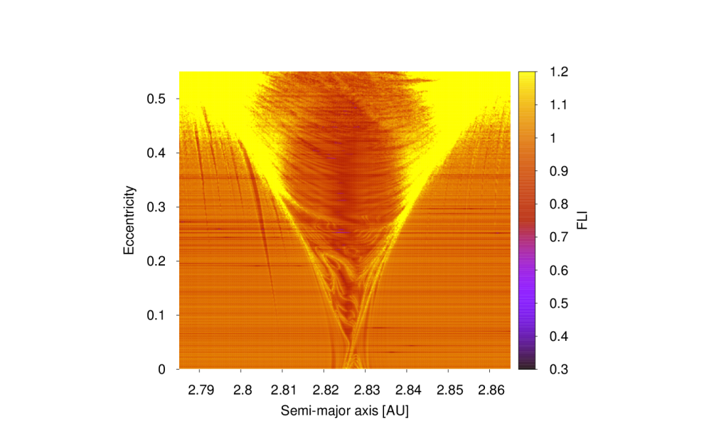
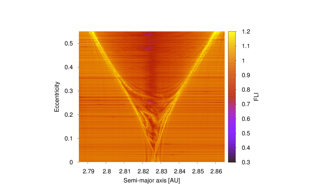
The most evident difference between the two plots is the amount of chaos. In the top panel, almost all particles out of the 5:2 MMR at higher are chaotic. The line of the resonant border becomes misshapen already at and a bunch of weak mean motion resonances arises from the chaotic upper part of the picture. In fact, a large number of resonances and their mutual overlapping generates all the chaos visible on the map. The bottom plot lacks chaos and a dense web of MMRs visible in the top panel. However, some weak thin vertical resonant-like shapes are visible in the lower panel as well. We do not identify all those resonances (it is beyond the scope of this paper and can be the subject of some future research) but a direct comparison between the two plots leads to the conclusion that resonances visible only in the top figure are MMRs generated by the inner planets - Venus, Earth or Mars. Following the same logic, weak resonances visible only in the bottom plot are caused by some of the outer planets.
We certainly do expect that the full Solar System model generates more chaos than the incomplete one, but having in mind the relatively small masses of the inner planets, the amount of chaos they produce for only 10 000 years is quite large.
The structure of chaos is clearly detected for eccentricities bellow , where many peculiarly shaped thin yellow lines are noticeable. Since their position and form remains unchanged on both plots, we conclude that the fine structure of chaos at low eccentricities is not affected by the presence of inner planets.
We consider a realistic model, which means that the observed structures should be placed exactly on the location we see on the plot. On the other hand, the orbital space is 6-dimensional, while the maps are 2-dimensional, i.e. the plots give a realistic, but only a partial insight into the chaotic structure of the 5:2 MMR. We notice that the peculiar structures look very similar to the traces of the hyperbolic invariant manifolds of the saddle point of the resonance, observed for example in Guzzo and Lega (2014, 2015). However, potential affiliation of those structures to the hyperbolic set requires a more detailed study and stronger theoretical grounds.
4 Evolution of 1000 test particles
The principal aim of this research is not only to illustrate the beauty of chaos in one of the most important Main Belt resonances, but also to show that the most unstable parts of the resonance do provide a fertile source of rapid delivery routes. For that purpose, we have chosen 1000 test particles initially placed along the chaotic structures visible on Fig. 1 and integrated them up to 5 Myr. We chose particles knowing a priori they would be ’active’ as soon the integration starts. In this way a significant reduction of calculation time can be achieved, since nominal integration times used in similar studies (Gladman et al, 1997; Bottke et al, 2002; de Leon et al, 2010) were much longer, up to 100 Myr. Initial semi-major axis and eccentricities of the particles are between and . Initial values of the remaining orbital elements are the same as for the computation of Fig. 1, that is .
The integrations were stopped if the orbit became hyperbolic or the particle reached semi-major axis larger than AU. The software used for integration (ORBIT9) deals well with planet close encounters, but it can not simulate collisions. Therefore, eventual planet-particle or particle-particle collision end states are not registered in the integration.
It should be noted that all our test bodies lie in the same inclination plane and have the same orbital angles. Therefore, the results presented reflect the migration abilities of a very small portion of the resonance. Selecting particles along all the 6 dimensions (or at least for different sets of the remaining 4 variables) would provide a more generic result on the 5:2 MMR diffusion capacities, but this approach is computationally very demanding, goes beyond the scope of this paper and will be the subject of further investigation.
5 Results
Considering that the 5:2 MMR is one of the best studied resonances in the Solar System, we will not repeat the known results on its dynamics, but rather focus on some new aspects of its transportation abilities. Since some results show a very large disagreement with previous studies on the 5:2 MMR, in addition (Table 1 in supplementary data) we list the exact values of the initial orbital elements of the 1000 test particles, so that the reader can reproduce the same integration. One part of Table 1 is given below.
| 2.8270400 | 0.0504400 | 2.8329999 | 0.1742000 |
| 2.8270800 | 0.0504400 | 2.8339601 | 0.1960400 |
| 2.8271201 | 0.0410800 | 2.8330400 | 0.1726400 |
| 2.8272400 | 0.0400400 | 2.8330801 | 0.1773200 |
| 2.8273201 | 0.0416000 | 2.8330801 | 0.1976000 |
| 2.8273602 | 0.0431600 | 2.8331201 | 0.1747200 |
| 2.8273602 | 0.0436800 | 2.8331201 | 0.1762800 |
| 2.8274400 | 0.0452400 | 2.8331201 | 0.1768000 |
| 2.8274400 | 0.0457600 | 2.8331201 | 0.2033200 |
| 2.8274801 | 0.0520000 | 2.8205600 | 0.1424800 |
| 2.8259602 | 0.0416000 | 2.8332000 | 0.1768000 |
| 2.8259602 | 0.0514800 | 2.8332000 | 0.1773200 |
| 2.8251200 | 0.0078000 | 2.8332000 | 0.1996800 |
| 2.8260000 | 0.0421200 | 2.8332400 | 0.2043600 |
| 2.8260000 | 0.0452400 | 2.8332801 | 0.2142400 |
| 2.8205600 | 0.1430000 | 2.8268800 | 0.0171600 |
| 2.8206401 | 0.1414400 | 2.8269200 | 0.0078000 |
| 2.8209600 | 0.1341600 | 2.8275201 | 0.0114400 |
| 2.8210402 | 0.1326000 | 2.8262801 | 0.0192400 |
| 2.8208802 | 0.1357200 | 2.8226800 | 0.1492400 |
| 2.8218000 | 0.1253200 | 2.8267601 | 0.0161200 |
| 2.8205600 | 0.1424800 | 2.8262401 | 0.0052000 |
5.1 Transportation to the NEO Region
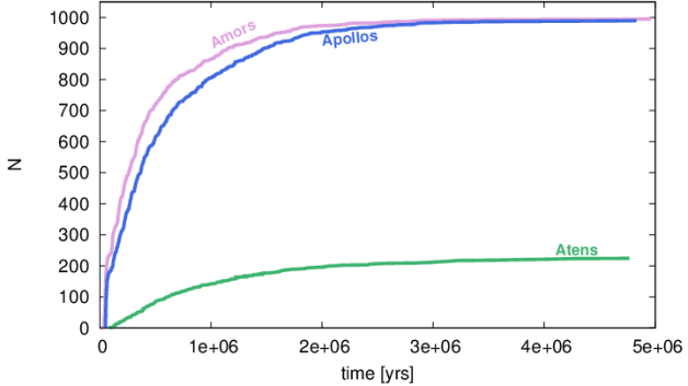
As many as of the test bodies became NEOs. More precisely, 995 out of 1000 particles at some moment reached perihelion distances smaller than AU. Statistical representation of the entry rates into the three NEO groups: Amors (), Apollos () and Athens () is given on Fig. 2.
The large amount of material migrating from the 5:2 resonance into the NEO region was not observed in earlier studies. For example, in Gladman et al (1997); Bottke et al (2002) or de Elía and Brunini (2007) this percentage was less than 10%. Such disagreement is primarily attributed to the way we choose initial conditions.
In order to illustrate this, we compare the chaoticity of test particles used in different studies. That is, we compute the FLI values of the initial data set used in this work, with the FLIs of the particles that were chosen in the same way as in Gladman et al (1997) and Bottke et al (2002). The three resulting histograms are given on Fig.3.
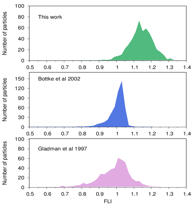
Considering the work of Gladman et al (1997), we sampled 1000 test bodies in between the borders of the 5:2 resonance in the region of the Gefion asteroid family and computed their FLI values for 10 000 yrs. The corresponding histogram is given in the bottom panel of Fig.3. The FLIs range between . Among them, as many as bodies have . We know from Fig.1 that such particles are not very chaotic, i.e. they are not the best candidates to drift rapidly through phase-space.
In Bottke et al (2002) the particles were sampled over a large part of the Outer Belt. For a detailed description of how the test bodies were selected, see section 2.5 in Bottke et al (2002). Following this description, we took 1000 asteroids with and from the Ted Bowell database (available at http://asteroid.lowell.edu) and computed their FLIs for the same amount of time, 10 000 years. The relevant histogram is given in the middle panel of Fig.3. Here FLIs range between and they have somewhat smaller diversity. A strong peak appears at , but only 5 asteroids are strongly chaotic having .
The FLI distribution of the 1000 particles used in this study is given on the top panel of Fig. 3. FLIs range between , but as many as bodies have FLIs larger than , i.e. a large majority is very chaotic justifying their fast migration abilities.
Time scales at which the 5:2 MMR increases eccentricities up to planet crossing values are similar to the ones observed in earlier studies. In both semi-analytical (Yoshikawa, 1991) and numerical studies (Ipatov, 1992; Morbidelli and Gladman, 1998) those times where estimated on years. Here, median time, i.e. time at which 50% of the particles became NEOs, is yrs. The mean time (arithmetical mean) of the first entry into the NEO region is yrs.
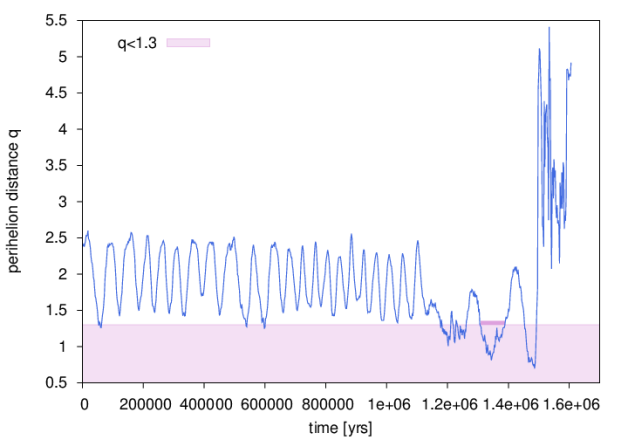
We are also interested to estimate the mean lifetime the objects spend in the NEO region. This estimation is often uncertain because most particles make multiple entries (and reentries). The situation is illustrated in Fig. 4, where we can follow the irregular behavior of the perihelion distance for one particle, along with its numerous entries into the NEO region (marked by the shaded area). The first time the object became a NEO was at yrs, but only for a few 100 yrs. The longest time it persisted below the NEO border was 80 000 yrs. In Fig. 4, this interval is marked with a bold line (at Myrs). The mean value of the first stay in the NEO region is relatively short, yrs. The mean value of the longest stay is Myr, comparable with the result from Bottke et al (2002) where this time was estimated on Myr.
5.2 Migration to the Sun
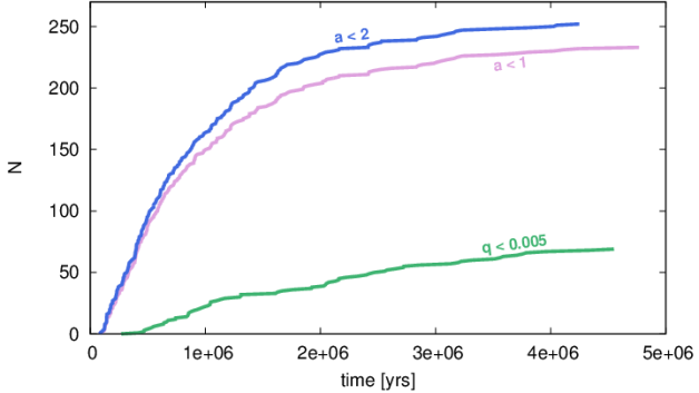
A large number of asteroids migrated closer to the Sun as well. Here we are able to directly compare (Table LABEL:table2) our results with the ones from Gladman et al (1997) and Bottke et al (2002). According to those studies, the 5:2 MMR was not capable of driving bodies to semi-major axis below AU. In our integration, this result is significantly different, as many as of the particles entered the AU region. A similar situation is observed for the orbits with AU, of the bodies at some point reached semi-major axis below AU, while in Bottke et al (2002) this fraction did not exceed .
| This work | Gladman et al 1997 | Bottke et al 2002 | |
| Number of particles | 1000 | 146 | 359 |
| Integration time (Myr) | 5 | 100 | 100 |
| Ever have AU (%) | 25.3 | 1.4 | <6 |
| Ever have AU (%) | 23.4 | 0 | - |
| Ever have AU (%) | 7 | 7.5 | - |
The rate of Sun-grazing bodies, i.e. bodies that have perihelion distances smaller than is . Among the 70 Sun grazers, 69 got there by increasing eccentricities close to 1, while only one particle actually approached the Sun due to the decrement of the semi-major axis down to 0. Therefore we can conclude that low values of are not affected by the decrease of . This could explain why we obtained almost the same result as Gladman et al (1997), where no particles with low have been observed, but the percent of bodies with was %, close to the value obtained in this study.
The entry rates into the regions with AU, AU and AU are given on Fig.5.
5.3 Close encounters
| Planet | (%) | |||
|---|---|---|---|---|
| Venus | 46.0 | |||
| Earth | 57.4 | |||
| Mars | 63.0 | |||
| Jupiter | 98.5 | |||
| Saturn | 67.3 | |||
| Uran | 42.6 | |||
| Neptune | 25.1 | |||
| no close enc. | 0.6 |
As mentioned above, the software we use does not register collisions (we do not treat any physical parameters required for those estimates). Therefore we ’simulate’ high collision probabilities by decreasing close approach distances down to 0. Our integrations are performed with nominal close approach distances ( AU for inner planets and AU for outer planets). Since an enormous number of close encounters was registered, we repeat the integration for smaller values of and .
That is, we set close approach distances to the radius of the Hill spheres of the planets ( AU for inner planets and AU for outer planets) and count the number of bodies entering the Hill spheres. It should be noted that changing close approach distances does not affect any other aspect of the evolved orbits (except that it counts close encounters), and that one particle usually has several planet rendezvous before it ends its journey through the Solar System.
In Table 3 we give the percentage of bodies entering the Hill sphere of each planet in the model. As expected, Jupiter dominates with bodies approaching it. The large amount of bodies getting close to it should not be a surprise, since most particles placed in the 5:2 MMR are ejected out of the system by Jupiter. The number of bodies approaching other planets decreases gradually as we move away from the resonance, both inwards and outwards the Solar System, while 6 particles stayed in the resonance avoiding any close encounters.
The amount of bodies entering the Hill sphere of Earth is very high, . This result was reconsidered in a new round of numerical integration, where the close approach distances were set to AU. We have found 5 bodies approaching Earth that close. The integrations were repeated for smaller values of , until no close encounters were registered. The lowest such limit was and two bodies were found to have approached Earth that close.
Although we were not able to estimate exact Earth collisional probabilities, the above result suggests that, if we choose particles at the most unstable parts of the resonance, the 5:2 resonance has at least one order of magnitude higher collisional probability with Earth, than the one observed in Morbidelli and Gladman (1998) or de Elía and Brunini (2007), where this value was estimated on .
5.4 Final destinations
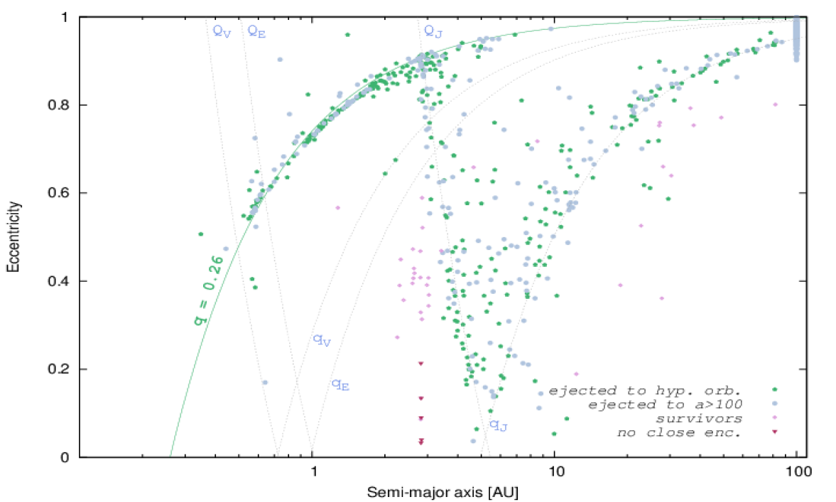
End states of the integrated particles are also under consideration. Distribution of their final positions in the plane is given in Fig. 6. The pink squares are the positions of the 42 survivors at the end of the integration. The 5 particles that stayed in the resonance and had not managed to raise up to planet crossing values are marked with purple triangles. The green dots (320 of them) are the locations from which the particles were ejected to hyperbolic orbits and the blue ones (638 of them) are the positions from which the bodies were thrown out to AU.
A large majority of those eliminations were caused by Jupiter, since most of the final positions are distributed along and in between the lines of its perihelion () and aphelion () distances. Some eliminations can be credited to other planets as well. For example, to Venus, the two green dots lying on the perihelion line at and or Earth, the blue dot on the line at . However, those removal scenaria confirm the expected and well known dynamical scheme of the 5:2 resonance. Median lifetimes of the particles (0.8 Myr) are in good agreement with previous results (Gladman et al, 1997).
The unexpected source of elimination is the sickle shaped line marked with a full green line. Since we have not found any resonance on that direction, it is uncertain if those removals are caused by some unknown resonance or another dynamical (or even numerical) mechanism. We have fitted a line through this removal course, which corresponds to the perihelion distance AU.
As mentioned above, all our test bodies lie in the same inclination plane and have the same values of the orbital angles. This could mean that the pathways along the AU are similar because the particles are taken from a narrow region inside the resonance. We repeat therefore the same integration (as described in Section 4) for other data sets, where the chaotic particles were selected for different combinations. It should be noted that the peculiar structures visible on Fig.1 were not observed in those cases (see Figures provided as supplementary material). We do not go into the details of statistical properties of those orbits, but focus on their final positions in the plane. Those positions are distributed in the same fashion as in Fig.6, including the elimination course along AU333See bottom panels in Fig. 10 and Fig. 11 in the supplementary material..
Thus, our results clearly suggest that the AU line may be a natural inner stability border of the NEO region. Let us recall a recent work of Granvik et al (2016), where it was found that NEOs do not survive certain low values of . As claimed by the authors, most such removals are credited to super-catastrophic breakups depending largely on the physical properties of NEOs (diameter, masses, albedo). Here we have observed a clear limitation in , although we do not consider any of those physical parameters. This leads to the conclusion that the disappearance of NEOs at low may also have a dynamical character.
According to Bottke et al (2002), a typical pathway of a test particle starting in the Main Belt could be illustrated by the following scheme:
where the so-called sink is a dynamical route along which most particles escape from the Solar System or fall on the Sun.
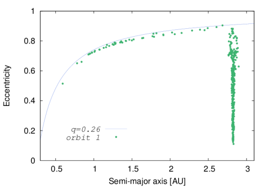
If we look at the orbital pathways of our individual test particles reaching low perihelion distances, we notice that most of the bodies travel along a direction close to the mentioned AU line. Therefore, we identify this line with the so called sink and modify the above scheme in the following way:
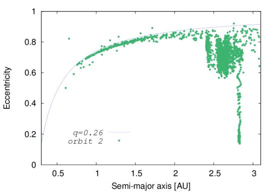
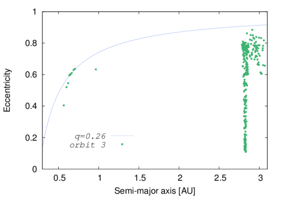
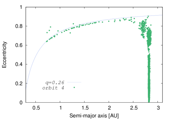
In order to illustrate this, we have randomly chosen four particles that reach low and have shown their orbital pathways in the plane in Fig. 7. The boundary is marked with a full line on all the four panels. Each of the four particles, after reaching high eccentricities and leaving the 5:2 resonance (or the neighboring resonances), navigates along a direction close to the course and leaves the system. Thus, the direction which we identified as a natural stability border, at the same time represents a dynamical highway along which particles travel to their final destination.
5.5 3200 Phaethon
In this final part, we will count the test bodies recovering the orbit of the asteroid (3200) Phaethon. That is, we search in the element space those particles that at some moment of the integration satisfy the following criteria , and , where are the semi-major axis, eccentricity and inclination of the asteroid (3200) Phaethon whose values are .
According to the results in Bottke et al (2002) Phaethon had a 0 probability of coming from the Jupiter family comets or Outer Belt region. This probability increased to 1% in the work of de Leon et al (2010). Among our 1000 test particles, we have found 80 bodies satisfying the above criteria, increasing this probability up to 8%.
6 Conclusions
The main results of this paper are summarized below.
-
•
We have computed dynamical maps of the 5:2 MMR for Solar System models with and without the inner planets. A direct comparison between them enabled a detection of weak neighboring resonances with inner planets.
-
•
We have observed chaotic structures inside the 5:2 resonance and we have illustrated that those structures represent a very effective source of transportation processes.
-
•
Time scales of the 5:2 MMR removal abilities are not significantly shortened, but the amount of material becoming NEOs (99.5% of the test bodies), reaching semi-major axis below 1 AU (23.4%) or entering the Hill sphere of Earth (57.4%) show a large disagreement with earlier studies. However, we point out that this mismatch is primarily attributed to the choice of initial conditions which are selected intentionally along the most unstable parts of the resonance that should have highly efficient transportation abilities.
-
•
The final destinations in the plane suggest that in addition to the main removal course caused by Jupiter, most particles are ejected out from an unknown direction defined with AU. Dynamical origin of this elimination line requires further investigation.
-
•
The percentage of our test particles that recovered a Phaethon like orbit is 8%.
Using sensitive numerical methods, we have shown that the 5:2 MMR with Jupiter has strong dynamical removal abilities that can drive a large amount of bodies in the close neighborhood of Earth. This result could explain the growing number of NEOs and meteorites that are identified as former members of the asteroid families located in the Outer Belt.
Applying this method on a single resonance enabled us to observe the ’hidden potential’ of its transportation abilities. Although the above results have to be analyzed further in future work, we conclude that extending the same method to other regions in the Solar System and other resonances could provide a clearer insight and a better understanding of the orbital migration phenomena.
Acknowledgements
This research was supported by the Ministry of Education, Science and Technological Development of the Republic of Serbia, under the project 176011 ’Dynamics and kinematics of celestial bodies and systems’. The calculations were performed on a Fermi cluster located at the Astronomical Observatory of Belgrade, purchased by the project III44002 ’Astroinformatics: Application of IT in astronomy and close fields’. The author is very grateful to the editor and an anonymous reviewer for their careful reading and constructive comments, which helped to improve the manuscript.
References
- Bazsó et al (2010) Bazsó, A., Dvorak, R., Pilat-Lohinger, E., Eybl, V., Lhotka, Ch., 2010, Celest.Mech.Dyn.Astr. 107, 63
- Bottke et al (2002) Bottke, W., Morbidelli, A., Jedicke, R., Petit, J-M., Levison, H., Michel, P. and Metcalfe, T., 2002, Icarus, 156, 399
- Daquin et al (2016) Daquin, J., Rosengren, A.J., Alessi, E.M., Deleflie, F., Valsecchi, G. and Rossi, A., 2016, Celest. Mech. Dynam. Astron.,124, 4, 335
- Dvorak et al (2003) Dvorak, R. et al., 2003, A&A, 398
- de Elía and Brunini (2007) de Elía, G.C., Brunini, A., 2007, A&A, 466, 1159
- Froeschlé et al (1997a) Froeschlé, Cl., Gonczi, R. and Lega, E., 1997, Planetary and Space Science, 45, 881
- Froeschlé et al (1997b) Froeschlé, Cl., Lega, E. and Gonczi, R.,1997, Celest. Mech. Dyn. Astron., 67, 41
- Froeschlé et al, (2005) Froeschlé, C., Guzzo, M. and Lega, E., 2005, Celest. Mech. Dynam. Astron., 92, 243
- Froeschlé et al, (2000) Froeschlé, C.,Guzzo, M. and Lega, E., 2000, Science, 289 N.5487:2108
- Galeş (2012) Galeş, C., 2012, Commun. Nonlinear. Sci. Numer. Simulat., 17, 4721
- Gladman et al (1997) Gladman, B.J., Migliorini, F., Morbidelli, A., Zappalá, V., Michel, P., Cellino, A., Froeschlé, C., Levison, H. F., Bailey, M., Duncan, M., 1997, Science, 277, 197
- Granvik et al (2016) Granvik, M., Morbidelli, A., Jedicke, R., Bolin, B., Bottke, W. F., Beshore, E., Vokrouhlický, D., Delbò, M. & Michel, P., 2016, Nature, 530, 303
- Guzzo (2005) Guzzo, M., 2005, Icarus, 174, 273
- Guzzo (2006) Guzzo, M., 2006, Icarus, 181, 475
- Guzzo and Lega (2014) Guzzo M. and Lega E., 2014, SIAM J. Appl. Math., 74, 4, 1058
- Guzzo and Lega (2015) Guzzo M. and Lega E., 2015, A&A, 579, A79, 1
- Ipatov (1992) Ipatov, S. I. 1992, Icarus, 95, 100
- Lega and Froeschlé (2003) Lega, E. and Froeschlé, C., 2003, Phys D, 182, 179
- de Leon et al (2010) de León, J., Campins, H., Tsiganis, K., Morbidelli, A. and Licandro, J., 2010, A&A, 513, A26
- Morbidelli and Gladman (1998) Morbidelli, A. and Gladman. B. 1998, Meteoritics Planet. Sci. 33, 999
- Nedelcu et al (2014) Nedelcu, D.A., Birlan, M., Popescu, M., Bădescu, O. and Pricopi, D., 2014 A&A 567, L7
- Nesvorný et al (2009) Nesvorný, D., Vokrouhlický, Morbidelli, A. and Bottke, W.F., 2009, Icarus, 200, 698
- Pilat-Lohinger et al (2002) Pilat-Lohinger, E. and Dvorak, R., 2002, Celest. Mech. Dynam. Astron. 82, 143
- Rabinowitz et al (1994) Rabinowitz, D. L., Bowell, E., Shoemaker, E. M. and Muinonen, K., 1994, (T. Gehrels and M. S. Matthews, Eds.), 285, Univ. of Arizona Tucson
- Rosengren (2015) Rosengren, A., Daquin,J., Alessi, E. M., Deleflie, F., Rossi, A., Valsecchi, G. B., 2015, arXiv:1512.05822
- Sándor (2007) Sándor, Z., Suli, A., Erdi, B., Pilat-Lohinger, E., Dvorak, R., 2007, Mon.Not.R.Astron.Soc.375, 1495
- Sanchez et al (2015) Sanchez, J.A, Reddy, V., Dykhuis, M., Lindsay, S. and Le Corre L., 2015, ApJ, 808, 93
- Schwarz (2011) Schwarz, R., Haghighipour, N., Eggl, S., Pilat-Lohinger, E. and Funk, B., 2011, Mon. Not. R. Astron. Soc. 414, 2763-2770
- Todorović et al (2008) Todorović, N., Lega, E., Froeschlé, C., 2008, Celest. Mech. Dynam. Astron., 102, 13
- Todorović et al (2011) Todorović, N., Guzzo, M., Lega, E. and Froeschlé, C., 2011, Celest. Mech. Dynam. Astron., 110, 389
- Todorović and Novaković (2015) Todorović, N. and Novaković, B., 2015, MNRAS, 451, 1637
- Vokrouhlický and Farinella (2000) Vokrouhlický, D. and Farinella, P., 2000, Nature, 407, 606
- Wetherill and Williams (1979) Wetherill, G. W., and Williams, J. G., 1979, In Origin and Distribution of the Elements (L. H. Ahrens, Ed.), 19 Pergammon, Oxford
- Wisdom (1983) Wisdom, J. 1983, Icarus 56, 51
- Yoshikawa (1991) Yoshikawa, M. 1991, Icarus, 92, 94