CC2 oscillator strengths within the local framework for calculating excitation energies (LoFEx)

Abstract

In a recent work [Baudin and Kristensen, J. Chem. Phys. 144, 224106 (2016)], we introduced a local framework for calculating excitation energies (LoFEx), based on second-order approximated coupled cluster (CC2) linear-response theory. LoFEx is a black-box method in which a reduced excitation orbital space (XOS) is optimized to provide coupled cluster (CC) excitation energies at a reduced computational cost. In this article, we present an extension of the LoFEx algorithm to the calculation of CC2 oscillator strengths. Two different strategies are suggested, in which the size of the XOS is determined based on the excitation energy or the oscillator strength of the targeted transitions. The two strategies are applied to a set of medium-sized organic molecules in order to assess both the accuracy and the computational cost of the methods. The results show that CC2 excitation energies and oscillator strengths can be calculated at a reduced computational cost, provided that the targeted transitions are local compared to the size of the molecule. To illustrate the potential of LoFEx for large molecules, both strategies have been successfully applied to the lowest transition of the bivalirudin molecule ($4255$ basis functions) and compared with time-dependent density functional theory.

I Introduction

High-accuracy calculations of electronic absorption spectra can be performed using coupled cluster (CC) response theoryKoch et al. (1995); Christiansen et al. (1996, 1998) via the computation of excitation energies and oscillator strengths. CC theory is well established as the method of choice for describing the electronic structure of molecules with a ground-state dominated by a single electronic configuration. However, the high-accuracy of CC models comes with a high computational cost and for that reason standard CC calculations of excitation energies and oscillator strengths have been limited to rather small molecules. Less reliable computational models like time-dependent density functional theory (TDDFT) are thus extensively used for the simulation of electronic spectra of medium-sized and large molecules.González, Escudero, and Serrano-Andrés (2012) We note that the equation-of-motion (EOM) CC formalism is closely related to CC response theory and is often used in the same context.Stanton and Bartlett (1993); Watts and Bartlett (1995); Gwaltney, Nooijen, and Bartlett (1996) While EOM and response techniques are identical for the calculation of CC excitation energies, we have chosen to consider CC response theory in this work since it results in size-intensive transition moments, in contrast to EOM-CC theory.Koch et al. (1994a)

The computational scaling of CC methods with the system size is associated with the usage of canonical Hartree-Fock (HF) orbitals which are generally delocalized in space, while CC theory describes local phenomena (electron correlation effects).Sæbø and Pulay (1993) In the last decades, a lot of efforts have been dedicated to the design of low-scaling CC models, primarily for the computation of ground-state energies.Sæbø and Pulay (1993); Werner and Schütz (2011); Yang et al. (2012); Riplinger et al. (2013); Eriksen et al. (2015); Werner et al. (2015); Riplinger et al. (2016); Li, Ni, and Li (2016); Nagy, Samu, and Kállay (2016); Friedrich (2012) More recently, several groups turned their attention to the calculation of excitation energies and molecular properties using local approximations. The combination of local occupied orbitals with non-orthogonal virtual orbitals (e.g. projected atomic orbitals (PAOs) or pair natural orbitals (PNOs)) is widely used to reduce the total number of wave function parameters and it has been applied to the calculation of excitation energies,Crawford and King (2002); Korona and Werner (2003); Kats, Korona, and Schütz (2006); Kats and Schütz (2009, 2010); Helmich and Hättig (2013, 2014); Dutta, Neese, and Izsák (2016) transition strengths,Kats, Korona, and Schütz (2007); Kats and Schütz (2010) and other molecular properties.Kats, Korona, and Schütz (2007); Crawford (2010); Kats and Schütz (2010); Russ and Crawford (2008); McAlexander and Crawford (2016) The incremental scheme in which the quantities of interest are expanded in a many-body series has also been applied to the calculation of CC excitation energiesMata and Stoll (2011) and dipole polarizabilities.Friedrich et al. (2015) Another recent development is the multilevel CC theory in which different CC models are used to treat different parts of the system.Myhre, Sánchez de Merás, and Koch (2013, 2014); Myhre and Koch (2016) In this context, we can also mention the reduced virtual space Send, Kaila, and Sundholm (2011) and ONIOM strategies.Caricato et al. (2010, 2011)

In a recent publication,Baudin and Kristensen (2016) we have introduced a new strategy for the calculation of CC excitation energies at a reduced computational cost, in which we focused on the second-order approximated CC singles and doubles (CC2) model. In our local framework for calculating excitation energies (LoFEx), the locality of correlation effects is used to generate a state-specific mixed orbital space composed of the dominant pair of natural transition orbitals (NTOs), obtained from time-dependent Hartree-Fock (TDHF) theory, and localized molecular orbitals (LMOs). This mixed orbital space is well adapted to describe the targeted electronic transition and can be significantly reduced (by discarding a subset of least relevant LMOs in a black-box manner) without affecting the accuracy of the calculated excitation energy. In this way, important computational savings are possible for local transitions in large molecular systems.

In Section II, we briefly summarize how excitation energies and oscillator strengths can be computed at the CC2 level of theory. The LoFEx algorithm for excitation energies is then summarized in Section III, in which we also suggest two different strategies for computing oscillator strengths within LoFEx. In Section IV, these strategies are compared when applied to the lowest electronic transitions of a set of medium-sized organic molecules. We also present results for a large molecule (bivalirudin) and compare the accuracy and computational efforts of LoFEx with TDDFT/CAM-B3LYP calculations.

II The RI-CC2 model for oscillator strengths

The CC2 model was introduced by Christiansen et al.Christiansen, Koch, and Jørgensen (1995) as an intermediate model between the CCS and CCSD models in the CC hierarchy for the calculation of frequency-dependent properties. CC2 is therefore the first model of the CC hierarchy to include correlation effects and thus constitutes an appropriate starting point for LoFEx. In this section, we summarize how CC2 excitation energies and oscillator strengths can be obtained from response theory.

The CC2 ground-state amplitudes are obtained as solution of the following non-linear equations,Christiansen, Koch, and Jørgensen (1995)

$$\Omega_{\mu_{1}} = \bra{\mu_{1}}\hat{H}+[\hat{H},T_{2}]\ket{\text{HF}}=0,$$ (1)

$$\Omega_{\mu_{2}} = \bra{\mu_{2}}\hat{H}+[F,T_{2}]\ket{\text{HF}}=0,$$ (2)

where $\{\ket{\text{HF}},\ket{\mu_{1}},\ket{\mu_{2}}\}$ denote the Hartree-Fock (HF) ground-state and the set of singles and doubles excitation manifolds. $F$ is the Fock operator and $\hat{H}$ is a similarity (T₁)-transformed Hamiltonian,

$$\hat{H}=\exp(-T_{1})H\exp(T_{1}),$$ (3)

where $T_{i}=\sum_{\mu_{i}}t_{\mu_{i}}\tau_{\mu_{i}}$ is a cluster operator, $t_{\mu_{i}}$ is a cluster amplitude, $\tau_{\mu_{i}}$ is an excitation operator, and $i$ denotes the excitation level. The $T_{1}$-transformation of the Hamiltonian in Eq. 3 can be transferred to the second-quantization elementary operators, which effectively corresponds to a modification of the molecular orbital (MO) transformation matrices $\mathbf{C}$ with the singles amplitudes,Koch et al. (1994b); Helgaker, Jørgensen, and Olsen (2000)

$$\begin{array}[]{rcl}X_{\alpha i}&=&C_{\alpha i}\\ Y_{\alpha i}&=&C_{\alpha i}+\sum_{a}C_{\alpha a}t^{a}_{i}\end{array}\qquad\begin{array}[]{rcl}X_{\alpha a}&=&C_{\alpha a}-\sum_{i}C_{\alpha i}t^{a}_{i}\\ Y_{\alpha a}&=&C_{\alpha a}\end{array}$$ (4)

A two-electron $T_{1}$-transformed integral in the Mulliken notation can now be expressed as,

$$(pq\hat{|}rs)= \sum_{\alpha\beta\gamma\delta}X_{\alpha p}Y_{\beta q}X_{\gamma r}Y_{\delta s}(\alpha\beta|\gamma\delta),$$ (5)

where we have used the following convention to denote orbitals:

• Atomic orbitals (AOs): $\alpha,\beta,\gamma\dots$

• MOs of unspecified occupancy: $p,q,r\dots$

• Occupied MOs: $i,j,k\dots$

• Virtual MOs: $a,b,c\dots$

Since only closed-shell molecules are targeted in this work, all MOs are considered spin-free.

In the CC2 model, the doubles amplitudes are only correct through first-order in the fluctuation potential ($\Phi=H-F$). This approximation leads to a closed-form of the doubles amplitudes,

$$t^{ab}_{ij}=\frac{(ai\hat{|}bj)}{\epsilon_{i}-\epsilon_{a}+\epsilon_{j}-\epsilon_{b}{}},$$ (6)

where $\epsilon_{p}$ denotes the orbital energy associated with orbital $p$. The CC2 equations can then be formulated in a CCS-like manner in which the doubles amplitudes are calculated on-the-fly. In order to take full advantage of this formulation and avoid the storage of any four-index quantity (amplitudes or integrals), Hättig and Weigend used the resolution-of-the-identity (RI) approximation for the two-electron integralsWhitten (1973); Feyereisen, Fitzgerald, and Komornicki (1993) both in the optimization of the CC2 ground-state and excitation amplitudes.Hättig and Weigend (2000) This strategy was later generalized to the calculation of transition strengths and excited-state first-order properties.Hättig and Köhn (2002)

In CC response theory, excitation energies and transition strengths from the ground-state ($0$) to an excited-state ($m$) are obtained from the poles and residues of the linear-response function, respectively.Christiansen, Jørgensen, and Hättig (1998) The poles of the CC linear-response function correspond to the eigenvalues of the non-symmetric Jacobian matrix,

$$A_{\mu_{i}\nu_{j}}=\partial\Omega_{\mu_{i}}/\partial t_{\nu_{j}},$$ (7)

while electric dipole transition strengths are given by,

$$S_{0m}^{V^{\mathfrak{j}}V^{\mathfrak{j}}} =T_{0m}^{V^{\mathfrak{j}}}T_{m0}^{V^{\mathfrak{j}}},$$ (8)

$$T_{0m}^{V^{\mathfrak{j}}} =\sum_{pq}[D_{pq}^{\eta}(\mathbf{R})+D_{pq}^{\xi}(\bar{\mathbf{M}})]\hat{V}^{\mathfrak{j}}_{pq},$$ (9)

$$T_{m0}^{V^{\mathfrak{j}}} =\sum_{pq}D_{pq}^{\xi}(\mathbf{L})\hat{V}^{\mathfrak{j}}_{pq},$$ (10)

where $\hat{V}^{\mathfrak{j}}_{pq}$ is a Cartesian component ($\mathfrak{j}=x,y,z$) of the T₁-transformed electric dipole integrals in the length gauge and $D_{pq}^{\eta}$ and $D_{pq}^{\xi}$ are one-electron density matrices (see Appendix A). $\mathbf{R}$ and $\mathbf{L}$ are the right and left Jacobian eigenvectors following the normalization condition $\mathbf{L}\mathbf{R}=1$ and $\bar{\mathbf{M}}$ are the transition moment Lagrangian multipliers. In addition, the ground-state Lagrangian multipliers $\bar{\mathbf{t}}$ are required for the calculation of the one-electron density matrices. As for the CC2 ground-state amplitudes, the CC2 excitation amplitudes and the Lagrange multipliers can be obtained without storing any four-index quantity by considering an effective Jacobian matrix,Hättig and Weigend (2000); Hättig and Köhn (2002)

$$A^{\text{eff}}_{\mu_{1}\nu_{1}}(\omega)=A_{\mu_{1}\nu_{1}}-\sum_{\gamma_{2}}\frac{A_{\mu_{1}\gamma_{2}}A_{\gamma_{2}\nu_{1}}}{\epsilon_{\gamma_{2}}-\omega},$$ (11)

where $\omega$ is an excitation energy and $\epsilon_{aibj}=\epsilon_{a}-\epsilon_{i}+\epsilon_{b}-\epsilon_{j}$. Using the effective Jacobian, the response equations to be solved become,

$$\mathbf{A}^{\text{eff}}{}(\omega)\mathbf{R}_{1}=\omega\mathbf{R}_{1},$$ (12)

$$\mathbf{L}_{1}\mathbf{A}^{\text{eff}}{}(\omega)=\mathbf{L}_{1}\omega,$$ (13)

$$\bar{\mathbf{t}}_{1}\mathbf{A}^{\text{eff}}{}(0)=-\bm{\eta}^{\text{eff}}_{1},$$ (14)

$$\bar{\mathbf{M}}_{1}(\mathbf{A}^{\text{eff}}{}(-\omega)+\omega\mathbf{1})=-\bar{\mathbf{m}}^{\text{eff}}_{1},$$ (15)

where the subscript $1$ denotes the singles part of a vector, and $\bm{\eta}^{\text{eff}}_{1}$ and $\bar{\mathbf{m}}^{\text{eff}}_{1}$ are the effective right-hand-sides of the linear equations for the ground-state and transition moments Lagrange multipliers, respectively. Once Eqs. 12, 13, 14 and 15 have been solved, the one-electron density matrices $D_{pq}^{\eta}$ and $D_{pq}^{\xi}$ can be calculated and contracted with $\hat{V}^{\mathfrak{j}}_{pq}$ to get the right and left transition dipole moments as well as transition strengths. All doubles quantities can be constructed on-the-fly whenever needed using the RI approximation for the two-electron integrals. In Appendix A we collect all the working equations required to calculate CC2 transition moments in a canonical MO basis. The equations are given here for completeness but should be equivalent to the ones in Ref. Hättig and Köhn, 2002. (A few typos were present in the original paper and are corrected in Appendix A).

When studying electronic transitions, one often consider oscillator strengths instead of the transition strengths given by Eq. 8. Oscillator strengths in the length gauge are straightforwardly obtained as,

$$f_{0m}=\frac{2}{3}\omega_{m}\sum_{\mathfrak{j}=x,y,z}S_{0m}^{V^{\mathfrak{j}}V^{\mathfrak{j}}},$$ (16)

where $\omega_{m}$ is the excitation energy for a transition from the ground-state to the $m$-th excited-state. The calculation of excitation energies and oscillator strengths at the CC2 level has been implemented in a local version of the LSDalton programAidas et al. (2014); lsd following the strategy presented in Refs. Hättig and Weigend, 2000 and Hättig and Köhn, 2002.

III Excitation energies and oscillator strengths within LoFEx

In a previous publicationBaudin and Kristensen (2016) we have introduced the LoFEx algorithm as a framework to calculate CC2 excitation energies of large molecules. In this section, we summarize the LoFEx procedure and extend it to the computation of CC2 oscillator strengths.

III.1 Excitation energies

In LoFEx a transition-specific orbital space is constructed based on the solutions of the TDHF problem for the whole molecule and starting from HF canonical molecular orbitals (CMOs). First, NTOs are obtained by performing a singular-value-decomposition (SVD) of the TDHF transition density matrix, $\mathbf{\widetilde{b}}$, for each transition of interest,Luzanov, Sukhorukov, and Umanskii (1976); Etienne (2015); Baudin and Kristensen (2016)

$$\mathbf{\widetilde{b}}^{\dagger}\mathbf{\widetilde{b}}\mathbf{u}_{k} =\lambda_{k}\mathbf{u}_{k},\quad k=1,2,\cdots,N_{o},$$ (17)

$$\mathbf{\widetilde{b}}\mathbf{\widetilde{b}}^{\dagger}\mathbf{v}_{k} =\lambda_{k}^{\prime}\mathbf{v}_{k},\quad k=1,2,\cdots,N_{v},$$ (18)

which leads to the transformation matrices from CMOs to NTOs for the occupied and virtual spaces, respectively,

$$\mathbf{U} =(\mathbf{u}_{1},\mathbf{u}_{2},\cdots,\mathbf{u}_{N_{o}}),$$ (19)

$$\mathbf{V} =(\mathbf{v}_{1},\mathbf{v}_{2},\cdots,\mathbf{v}_{N_{v}}),$$ (20)

Where $N_{o}$ ($N_{v}$) is the number of occupied valence (virtual) orbitals. Assuming $N_{o}\leq N_{v}$, it follows that $\lambda_{k}\equiv\lambda_{k}^{\prime}$ for $k=1,2,\cdots,N_{o}$, while $\lambda_{k}^{\prime}=0$ for $k=N_{o}+1,\cdots,N_{v}$. The relevance of a given pair of NTOs ($k$) in the electronic transition associated with the density matrix $\mathbf{\widetilde{b}}$ can be evaluated through its singular value $\sqrt{\lambda_{k}}$.Luzanov, Sukhorukov, and Umanskii (1976); Martin (2003) For singles-dominated transitions, one pair of NTOs (with singular value close to one) dominates the transition, while the other NTOs are far less important to describe the process and thus have much smaller singular values. In LoFEx we therefore keep the dominant pair of NTOs intact, while the remaining orbitals are localized using the square of the second central moment of the orbitals as a localization function.Jansík et al. (2011); Høyvik, Jansík, and Jørgensen (2012) This procedure (summarized in the upper part of Fig. 1) results in a mixed orbital space composed of orthogonal NTOs and localized molecular orbitals (LMOs) that is adapted to the description of a specific electronic transition. Core orbitals are not considered in the generation of NTOs and are localized independently to avoid mixing between core and valence spaces.

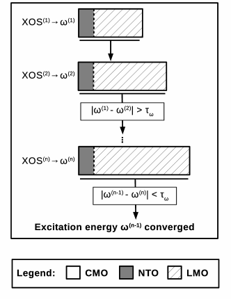
Figure 1: Schematic representation of the original LoFEx procedure. $\mathbf{U}$ and $\mathbf{V}$ represent the transformation matrices from canonical molecular orbitals (CMOs in white) to natural transition orbitals (NTOs in grey) for the valence and virtual spaces, respectively. $\mathbf{\widetilde{C}}$, $\mathbf{\widetilde{U}}$, and $\mathbf{\widetilde{V}}$ represent the transformation matrices to local molecular orbitals (LMOs in stripes) for core, valence, and virtual orbitals, respectively, excluding the dominant pair of NTOs. $\tilde{r}_{p}$ is the effective distance measure given by Eq. 21, $\omega^{(i)}$ is the excitation energy corresponding to the $i$-th excitation orbital space (XOS⁽ⁱ⁾) and $\tau_{\omega}$ is the LoFEx excitation energy threshold.

In this mixed orbital space, the dominant pair of NTOs is expected to describe the main character of the targeted electronic transition, while the LMOs enable an efficient description of correlation effects. In order to reduce the computational cost of the CC calculation, a subspace of the mixed NTO/LMO space is then constructed by considering the most relevant orbitals based on an effective distance $\tilde{r}_{p}$ given by,

$$\tilde{r}_{p}=\min_{A}\left(\frac{r_{Ap}}{Q^{\text{NTO,o}}_{A}},\frac{r_{Ap}}{Q^{\text{NTO,v}}_{A}}\right),$$ (21)

where index $A$ denotes atomic centers, $r_{Ap}$ corresponds to the distance between the center of charge of a local orbital $p$ and atomic center $A$, and $Q^{\text{NTO,o}}_{A}$ and $Q^{\text{NTO,v}}_{A}$ are the Löwdin atomic charges of the occupied and virtual NTOs on center $A$, respectively. The resulting reduced space is denoted the excitation orbital space (XOS). The inactive Fock matrix can then be diagonalized in the XOS to obtain a set of pseudo-canonical orbitals. CC excitation energies (and eventually oscillator strengths) can then be calculated in the XOS using standard canonical implementations, as described in Section II and Appendix A for the CC2 model.

In order to preserve the black-box feature of CC theory, the XOS is optimized as depicted in the lower part of Fig. 1, i.e., a first guess for the XOS (XOS⁽¹⁾) is built and the CC problems are solved in that space to provide the excitation energy $\omega^{(1)}$, the XOS is then extended based on the list defined by Eq. 21 until the difference between the last two excitation energies is smaller than the LoFEx excitation energy threshold $\tau_{\omega}$, ($|\omega^{(n-1)}-\omega^{(n)}|<\tau_{\omega}$). We have shown in Ref. Baudin and Kristensen, 2016 (where $\tau_{\omega}$ was denoted $\tau_{\text{XOS}}$), that this procedure can result in significant speed-ups compared to standard CC2 implementations without loss of accuracy.

III.2 Oscillator strengths

For the calculation of oscillator strengths with LoFEx, we consider the following strategies:

1. The XOS is optimized solely based on the excitation energy (as described in Fig. 1 and Ref. Baudin and Kristensen, 2016) and the oscillator strength is only calculated once in the optimized XOS (XOS^(n-1)).

2. Both excitation energies and oscillator strengths are calculated in each LoFEx iteration and only the oscillator strength is checked for convergence. In other words, the XOS is considered converged when, $|f^{(n)}-f^{(n-1)}|<\tau_{f}$, where $\tau_{f}$ is the LoFEx oscillator strength threshold.

Note that in the XOS optimization, the last step (step $n$) is necessary to check that step $n-1$ was already converged. The calculation of oscillator strengths in point 1 is therefore done in the penultimate XOS to ensure minimal computational efforts.

In the following section, we will refer to point 1 as the standard-LoFEx strategy, while point 2 is denoted the spectrum strategy. Indeed, in point 2 the oscillator strength threshold $\tau_{f}$ has a different purpose than the excitation energy threshold $\tau_{\omega}$. Checking only the oscillator strength for convergence is expected to provide a balanced description of the transitions in the sense that transitions with large oscillator strengths should be well described, while weak transitions (with $f\simeq 0$) are expected to converge in minimal XOSs and lead to less accurate excitation energies, while using less computational resources. The standard-LoFEx strategy is thus preferred if accurate excitation energies are requested for all transitions, while the spectrum strategy is more appropriate if one is only interested in transitions with a significant oscillator strengths.

IV Results

In this section we present numerical results for excitation energies and oscillator strengths using the standard- and spectrum-LoFEx strategies introduced in Section III. For that purpose, we consider the following set of medium-sized organic molecules,

• caprylic acid,

• lauric acid,

• palmitic acid,

• 15-oxopentadecanoic acid (15-OPDA),

• prostacyclin,

• an $\alpha$-helix composed of 8 glycine residues ($\alpha$-Gly₈),

• leupeptin,

• latanoprost,

• met-enkephalin, and

• 11-cis-retinal.

The molecular geometry for 11-cis-retinal was obtained from Ref. Dutta, Neese, and Izsák, 2016, while for the other systems, the Cartesian coordinates as well as details regarding the optimization of the structures are available in Ref. Baudin and Kristensen, 2016 and its supporting information. All the calculations presented in this section have been performed with a local version of the LSDalton program,lsd ; Aidas et al. (2014) using the correlation consistent aug-cc-pVDZ’ basis setDunning Jr. (1989); Kendall, Dunning Jr., and Harrison (1992) with the corresponding auxiliary basis, aug-cc-pVDZ-RI’ for the RI approximation.Weigend, Köhn, and Hättig (2002) The prime in the basis set notation indicates that diffuse functions have been removed on the hydrogen atoms.

The parameters used in the following investigation have been set to the same default values as in Ref. Baudin and Kristensen, 2016, i.e., the LoFEx excitation energy threshold was set to $\tau_{\omega}=0.02$ eV and the number of orbitals added to the XOS in each LoFEx iteration corresponds to ten times the average number of orbitals per atom. For the spectrum-LoFEx strategy we have chosen $\tau_{f}=0.001$.

IV.1 Calculation of oscillator strengths within LoFEx

Table 1: Comparison of standard-LoFEx ($\tau_{\omega}=0.02$ eV) and conventional CC2 excitation energies and oscillator strengths. The LoFEx excitation energies are given in eV for the largest XOS (step $n$) and for the converged XOS (step $n-1$), while oscillator strengths are only reported for the converged XOS. Absolute errors are given for both excitation energies and oscillator strengths. Finally, the number of iterations in the XOS optimization ($n$) as well as speed-ups of LoFEx compared to conventional CC2 algorithms are also reported.

System	State	No. iter. $(n)$	$\omega^{(n)}$	$\delta\omega^{(n)}$	$\omega^{(n-1)}$	$\delta\omega^{(n-1)}$	$f^{(n-1)}$	$\delta f^{(n-1)}$	Speed-up
Caprylic acid	S1	2	6.06	0.00	6.07	0.01	0.000	0.000	0.72
	S2	3	6.83	0.00	6.83	0.00	0.066	0.003
Lauric acid	S1	3	6.05	0.00	6.06	0.00	0.000	0.000	1.29
	S2	3	6.81	0.00	6.82	0.01	0.065	0.005
Palmitic acid	S1	3	6.06	0.00	6.06	0.00	0.000	0.000	4.07
	S2	3	6.81	0.01	6.83	0.03	0.065	0.005
15-OPDA	S1	2	4.44	0.00	4.45	0.01	0.000	0.000	1.52
	S2	2	6.06	0.00	6.08	0.02	0.000	0.000
	S3	5	6.19	0.00	6.19	0.00	0.040	0.001
Prostacyclin	S1	5	4.98	0.00	4.99	0.01	0.005	0.000	1.16
$\alpha$-gly8	S1	4	5.43	0.00	5.43	0.00	0.001	0.000	2.46
	S2	4	5.73	0.00	5.73	0.01	0.003	0.001
Leupeptin	S1	3	4.27	0.01	4.28	0.01	0.001	0.000	3.37
Latanoprost	S1	3	5.08	0.00	5.08	0.01	0.001	0.000	16.8
Met-enkephalin	S1	3	4.78	0.00	4.79	0.01	0.024	0.002	34.0
11-cis-retinal	S1	5	2.14	0.00	2.14	0.00	1.384	0.000	0.61

In Table 1 we report the LoFEx excitation energies and oscillator strengths for the lowest electronic transitions of the molecules presented above when using the standard-LoFEx strategy. Absolute errors in the excitation energies and the oscillator strengths as well as speed-ups compared to conventional CC2 implementations are also reported. Since in the standard-LoFEx strategy, the oscillator strength is only calculated in the converged (penultimate) XOS, we report excitation energies corresponding to both the expanded (step $n$) and converged (step $n-1$) XOSs. We note that, as demonstrated in Ref. Baudin and Kristensen, 2016, the excitation energies in the expanded steps are “overconverged” (all errors are well below $0.02$ eV), while in the penultimate steps the errors in the excitation energies are of the order of the LoFEx excitation energy threshold ($0.02$ eV). For the oscillator strengths, the absolute errors are equal or below $0.005$ and are strongly correlated with the intensity of the transitions (larger oscillator strengths correspond to larger errors), except for 11-cis-retinal which include the complete orbital space.

Regarding the speed-ups of the standard-LoFEx algorithm compared to a conventional (multi-state) CC2 implementation, it is found that the state-specific approach of LoFEx remains advantageous in most cases, even for the computation of several transitions. This is of course strongly dependent on the character of the transitions and on the size of the molecule, e.g. in the case of 15-OPDA, the two lowest transitions are rather local and converge in only two LoFEx iterations but the third transition has a more delocalized characterBaudin and Kristensen (2016) and requires almost the complete orbital space to be included in the XOS which limits significantly the obtained speed-up ($1.52$). Another less favorable case for LoFEx is the lowest transition of 11-cis-retinal. Both the excitation energy and the oscillator strength are perfectly recovered by LoFEx. However, the complete orbital space is required in order to determine the excitation energy to the desired precision, and the oscillator strength thus also has to be calculated in the complete orbital space, which results in a “speed-up” of $0.61$. This behaviour can be understood by looking at the dominant pair of NTOs in Fig. 2, which shows that the transition is basically affecting the whole molecule, preventing any computational savings using LoFEx. This should be put in contrast with the performance of LoFEx for the met-enkephalin molecule, where both the excitation energy and the oscillator strength are well described with only 3 LoFEx iterations, resulting in a significant speed-up ($34$). It should be emphasized that the gain in terms of computational efforts for met-enkephalin is much greater than the computational overhead observed for 11-cis-retinal. These two examples demonstrate that LoFEx is designed to ensure error control and accuracy of the results, while computational savings are transition and system dependent.

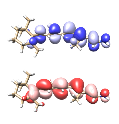
Figure 2: Stick representation of the 11-cis-retinal molecule. Natural transition orbitals for the lowest transition are represented with a contour value of $0.02$ a.u. (bottom: occupied NTO, top: virtual NTO).Pettersen et al. (2004)

Table 2: Comparison of spectrum-LoFEx ($\tau_{f}=0.001$) and conventional CC2 excitation energies and oscillator strengths. The LoFEx excitation energies and the corresponding absolute errors are given in eV. We also report the oscillator strengths and corresponding absolute errors as well as the number of iterations used in the XOS optimization ($n$) and the speed-ups of LoFEx compared to conventional CC2 algorithms.

System	State	No. iter. $(n)$	$\omega^{(n)}$	$\delta\omega^{(n)}$	$f^{(n)}$	$\delta f^{(n)}$	Speed-up
Caprylic acid	S1	1	6.07	0.01	0.000	0.000	0.65
	S2	3	6.82	0.00	0.069	0.000
Lauric acid	S1	1	6.08	0.02	0.000	0.000	0.79
	S2	4	6.81	0.00	0.070	0.000
Palmitic acid	S1	1	6.09	0.04	0.000	0.000	0.88
	S2	5	6.80	0.00	0.070	0.000
15-OPDA	S1	1	4.45	0.01	0.000	0.000	0.97
	S2	1	6.08	0.02	0.000	0.000
	S3	5	6.19	0.00	0.040	0.001
Prostacyclin	S1	5	4.98	0.00	0.005	0.000	0.71
$\alpha$-gly8	S1	2	5.46	0.03	0.001	0.000	11.1
	S2	2	5.76	0.04	0.004	0.002
Leupeptin	S1	1	4.30	0.04	0.000	0.001	69.0
Latanoprost	S1	3	5.07	0.00	0.001	0.000	9.31
Met-enkephalin	S1	4	4.78	0.00	0.022	0.000	5.01
11-cis-retinal	S1	5	2.14	0.00	1.384	0.000	0.42

With the idea of producing electronic spectra of CC2 quality at a reduced computational cost, we now turn our attention to the spectrum-LoFEx strategy. In electronic spectra, it is important to provide a good description of the transitions with large oscillator strengths and, for that purpose, the standard-LoFEx strategy might be inappropriate since it converges the XOS based on the excitation energies and not on the oscillator strengths. In Table 2 we report the LoFEx excitation energies and oscillator strengths for the lowest electronic transitions of the molecules presented above when the spectrum-LoFEx strategy is used with $\tau_{f}=0.001$. Absolute errors in the excitation energies and the oscillator strengths as well as speed-ups compared to conventional CC2 implementations are also reported. Since in the spectrum-LoFEx strategy, the oscillator strengths and excitation energies are calculated in each LoFEx iteration, we only report the values corresponding to the most accurate results, i.e., the ones from the expanded XOS (step $n$). Note also that, while in the standard-LoFEx procedure at least two steps are necessary to check the convergence of excitation energies ($n\geq 2$), in the spectrum strategy we consider that the first step can be directly converged if $f^{(1)}<\tau_{f}$.

From Table 2, we see that for the strongest transitions (with $f>0.01$) the errors in both the excitation energies and the oscillator strengths are very satisfactory. As expected, for weaker transitions, larger errors occur in the excitation energies (up to $0.04$ eV) which is related to the fact that only the oscillator strengths are used to converge the XOS. For example, for the lowest transition of leupeptin ($f=0.001$ and $\delta\omega=0.04$), the weak character of the transition leads to a converged XOS in the first iteration and a significant speed-up ($69.0$) is observed. However, the results in Table 2 also show that, even if some computational time is saved on the weakest transitions, more time has to be dedicated to the stronger ones since larger XOSs are required to achieved the desired accuracy and since the oscillator strengths have to be calculated in each LoFEx iteration. As a consequence, less impressive speed-ups are observed for the spectrum-LoFEx strategy (except for $\alpha$-gly₈ and leupeptin). However, as for the standard-LoFEx strategy in Table 1 we note that the potential speed-ups are much larger than the additional overhead present in the less favorable cases.

Comparing Tables 1 and 2 we note that for all the transitions with $f>0.01$, the number of required iterations with the spectrum strategy is always larger or equal to the number of iterations used in the standard-LoFEx strategy. In accordance with Ref. Kats, Korona, and Schütz, 2007, this suggests that a fine-tuned description of (strong) oscillator strengths requires larger orbital spaces than the excitation energy alone. Finally, we note that both the accuracy and the computational savings are driven by the main LoFEx threshold ($\tau_{f}$ for the spectrum strategy) and that in practical applications of LoFEx, $\tau_{f}$ could of course be increased to reduce the computational efforts at the expense of obtaining slightly less accurate oscillator strengths.

IV.2 Large-scale application: the bivalirudin molecule

In order to demonstrate the potential of LoFEx for large molecules, we apply both the standard and spectrum strategies for the calculation of the lowest excitation energy and the corresponding oscillator strength of the bivalirudin molecule (see Fig. 3). Bivalirudin is a synthetic polypeptide containing $20$ residues. The structure used in this paper was obtained from the ChemSpider database, hydrogen atoms were added and the geometry was relaxed at the molecular mechanics level (MMFF94Halgren (1996) force field) using Avogadro.Hanwell et al. (2012)^, The Cartesian coordinates of the optimized structure are available in the supporting information. The calculations have been performed using the cc-pVDZ and aug-cc-pVDZ’ basis sets which (for the whole molecule) contain $2860$ and $4255$ basis functions, respectively.

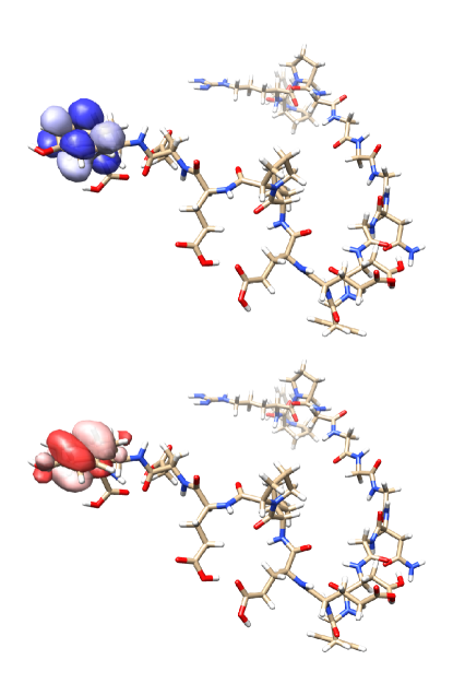
Figure 3: Stick representation of the bivalirudin molecule. Natural transition orbitals for the lowest transition are represented with a contour value of $0.02$ a.u. (bottom: occupied NTO, top: virtual NTO).Pettersen et al. (2004)

Table 3: LoFEx CC2 calculations of excitation energies and oscillator strengths for the lowest transition of the bivalirudin molecule. For standard-LoFEx, $\tau_{\omega}=0.02$ eV and we report values for $\omega^{(n)}$ and $f^{(n-1)}$, while for spectrum-LoFEx, $\tau_{f}=0.001$ and we report values for $\omega^{(n)}$ and $f^{(n)}$. For comparison TDDFT/CAM-B3LYP results are also reported. Timings are given in hours for all calculations and the fraction of time spent in the CC part of the LoFEx calculations is given in % as $T_{\text{CC/tot}}$.

Basis set	method	No. iter. $(n)$	$\omega$	$f$	Time (hours)	$T_{\text{CC/tot}}$
cc-pVDZ	standard-LoFEx	3	4.98	0.030	7	3.2
	spectrum-LoFEx	4	4.98	0.029	8	15
	CAM-B3LYP	—	5.14	0.034	13	—
aug-cc-pVDZ’	standard-LoFEx	3	4.82	0.028	157	1.4
	spectrum-LoFEx	4	4.82	0.026	164	5.5
	CAM-B3LYP	—	5.01	0.029	205	—

One of the goals of LoFEx is to provide CC results with a computational cost that can compete with TDDFT. In order to evaluate this feature for the bivalirudin calculations, we have performed TDDFT/CAM-B3LYPRunge and Gross (1984); Casida (1995); Yanai, Tew, and Handy (2004) calculations using the same basis sets and targeting the same transition as for the LoFEx calculations. We note that for a fair comparison, the density-fittingWhitten (1973); Baerends, Ellis, and Ros (1973); Reine et al. (2008) approximation for the Coulomb integrals was used in both the TDDFT calculations and in the TDHF part of LoFEx. We have also performed the LoFEx calculations without density-fitting in the TDHF part and verified that the final LoFEx-CC2 results were not affected by this approximation (to the desired precision). Note, that the calculations in Section IV.1 were performed without using density-fitting in the TDHF part of LoFEx. In Table 3, we report timings for LoFEx as well as for the TDDFT calculations. For LoFEx, we also report the fraction of the time (in %) spent in the CC part of the calculations denoted $T_{\text{CC/tot}}$. All the calculations reported in Table 3 were performed on Dell C6220 II compute-nodes, with 2 ten-core Intel E5-2680 v2 CPUs @ 2.8 GHz and 128 GB of memory.

Regarding the computational efforts in LoFEx, the values for $T_{\text{CC/tot}}$ in Table 3 indicates that only a few percents of the time is spent in the CC2 part of the calculations. In the best case, for the standard-LoFEx/aug-cc-pVDZ’ result only $1.4$ % is spent in the CC2 algorithm, while $15$ % are used in the spectrum-LoFEx/cc-pVDZ calculation. Of course, for a given type of transition, the larger the molecule, the smaller $T_{\text{CC/tot}}$ would be. This indicates that, as expected, LoFEx effectively enables CC calculations of excitation energies and oscillator strengths at roughly the cost of a TDHF calculation, provided that the transition of interest is local compared to the size of the molecule. In fact, the LoFEx calculations are between $1.2$ and $1.9$ times faster than the corresponding TDDFT/CAM-B3LYP calculations.

In Table 3, we also report the excitation energies and oscillator strengths obtained with the different methods (TDDFT and LoFEx). Both LoFEx strategies give the same excitation energies for which a red-shift of $0.16$ eV is observed when adding diffuse functions in the basis set. The TDDFT numbers lie $0.16$ and $0.19$ eV higher than the CC2 excitation energies for the cc-pVDZ and aug-cc-pVDZ’ basis sets, respectively, which shows reasonably good agreement between the two methods. As expected, the values for the oscillator strengths are slightly more dependent on the choice of the LoFEx strategy. Since CC2 reference numbers are out of reach, one should consider the results of the spectrum-LoFEx strategy to be superior (it takes one more iteration to converge). The TDDFT oscillator strengths are slightly higher for both basis sets but still very close to the CC2 results.

V Conclusion

In this paper we have presented an extension of the LoFEx algorithm to the computation of oscillator strengths using CC2 linear-response theory. In LoFEx, a state-specific mixed orbital space is generated from a TDHF calculation on the whole molecule by considering the dominant pair of NTOs, while the remaining orbitals are localized. A reduced excitation orbital space (XOS), is then determined in a black-box manner for each electronic transition. Two different strategies have been suggested for the computation of oscillator strengths within LoFEx: a standard strategy in which the XOS is optimized solely based on the CC2 excitation energy, while the oscillator strength is only calculated in the converged (penultimate) XOS, and a spectrum strategy which performs the XOS optimization directly based on the oscillator strength. The first approach is designed to provide accurate excitation energies for all targeted transitions, while the second strategy is dedicated to the calculation of electronic spectra, such that strong transitions are described accurately, while less computational efforts are spent on weak and forbidden transitions.

Both strategies have shown promising results in terms of accuracy when applied to a set of medium-sized organic molecules. Significant computational savings with respect to conventional CC2 implementations are obtained whenever the considered transitions are local compared to the size of the molecule. However, we note that for the strongest transition investigated in this work (S₁ of 11-cis-retinal), no computational savings could be obtained due to the delocalized electronic structure of the molecule. Many spectroscopically interesting chromophores have a delocalized electronic structure,Jacquemin, Duchemin, and Blase (2015) and for such species, little or no computational savings would be obtained using LoFEx. In order to extend the applicability of LoFEx, it might therefore be necessary to further reduce the size of the XOS by considering, e.g., pair natural orbitals (PNOs),Helmich and Hättig (2013); Dutta, Neese, and Izsák (2016) or improved NTOs. This issue will be addressed in future publications. Nonetheless, the current LoFEx algorithm could be applied successfully to the bivalirudin molecule with $4255$ basis functions, demonstrating that for transitions that are local compared to the size of the molecule, LoFEx can provide CC2 excitation energies and oscillator strengths at a computational cost competing with that of TDDFT.

Appendix A Working equations for CC2 transition moments

In this appendix we summarize the working equations of the CC2 model for the calculation of excitation energies and (ground-state to excited-state) transition moments for closed-shell molecules. For the derivation of those equations we have considered spin-free canonical orbitals and the following biorthonormal basis,Helgaker, Jørgensen, and Olsen (2000)

$$\Bra{{}^{ab}_{ij}} =\Bra{\text{HF}}E_{jb}E_{ia},$$ (22a)

$$\Ket{{}^{ab}_{ij}} =E_{ai}E_{bj}\Ket{\text{HF}},$$ (22b)

$$\Bra{\widetilde{{}^{ab}_{ij}}} =\frac{1}{1+\delta_{ai,bj}}\left(\frac{1}{3}\Bra{{}^{ab}_{ij}}+\frac{1}{6}\Bra{{}^{ab}_{ji}}\right),$$ (22c)

$$\Braket{\widetilde{{}^{ab}_{ij}}}{{}^{cd}_{kl}} =\delta_{aibj,ckdl},$$ (22d)

where $E_{ai}$ is a singlet excitation operator in second-quantization. The singles and doubles cluster operators are then defined as follows,

$$T_{1}=\sum_{ai}t^{a}_{i}E_{ai},$$ (23)

$$T_{2}=\frac{1}{2}\sum_{aibj}t^{ab}_{ij}E_{ai}E_{bj}.$$ (24)

In the following section we only provide the CC2 working equations, for the details regarding the algorithm and the use of the RI approximation for the two-electron repulsion integrals, we refer to Refs. Hättig and Weigend, 2000; Hättig and Köhn, 2002.

A.1 Overview

The computation of transition moments from CC2 linear-response theory can be performed as follows (all the intermediate quantities are given in the following sections),

1. Determine the ground-state singles amplitudes $t^{a}_{i}$ from Eq. (1) and using Table 5 (left).

2. Determine the ground-state singles Lagrangian multipliers $\bar{t}^{a}_{i}$ from Eq. 14 and using Table 6 (left) with $\omega=0$ and with the right-hand-side from Eq. 43.

3. Determine the “right” singles excitation amplitudes $R^{a}_{i}$ from Eq. 12 and using Table 5 (right).

4. Determine the “left” singles excitation amplitudes $L^{a}_{i}$ from Eq. 13 and using Table 6 (left).

5. Check that right and left excitation energies agree to the desired precision and normalize the excitation vectors using Eqs. 46 and 47,

   $$\sum_{ai}L^{a}_{i}R^{a}_{i}+\frac{1}{2}\sum_{aibj}L^{ab}_{ij}R^{ab}_{ij}=1$$ (25)

6. Determine the transition moment Lagrangian multipliers $\bar{M}^{a}_{i}$ from Eq. 15 and using Table 6 (left). The right-hand-side has to be computed beforehand from Table 6 (right) which requires the optimized right excitation amplitudes and the ground-state Lagrangian multipliers. The corresponding doubles quantities are computed on-the-fly from Eqs. 46, 51 and 48.

7. Compute the one-particle density matrices given in Section A.5 using the doubles quantities in Section A.4.

8. The density matrices can then be contracted with electric dipole moment T₁-transformed integrals to get the transition strengths as in Eqs. 8, 9 and 10.

A.2 Integrals and Fock matrices

We write two-electron repulsion integrals in the Mulliken notation as,

$$(pq|rs)=\sum_{\alpha\beta\gamma\delta}C_{\alpha p}C_{\beta q}C_{\gamma r}C_{\delta s}(\alpha\beta|\gamma\delta)$$ (26)

where the $C_{\alpha p}$ are Hartree-Fock canonical MO coefficients.

A general inactive Fock matrix is given by

$$F_{pq}= h_{pq}+\sum_{i}[2(pq|ii)-(pi|iq)]=\delta_{pq}\epsilon_{p}$$ (27)

$$h_{pq}= \sum_{\alpha\beta}C_{\alpha p}C_{\beta q}h_{\alpha\beta}$$ (28)

where we have introduced the one-electron integrals $h_{pq}$ and Hartree-Fock orbital energies $\epsilon_{p},\epsilon_{q}\dots$

We consider integrals transformed with the singles ground-state amplitudes,

$$(pq\hat{|}rs)= \sum_{\alpha\beta\gamma\delta}X_{\alpha p}Y_{\beta q}X_{\gamma r}Y_{\delta s}(\alpha\beta|\gamma\delta)$$ (29)

$$\hat{h}_{pq}= \sum_{\alpha\beta}X_{\alpha p}Y_{\beta q}h_{\alpha\beta}$$ (30)

$$\begin{array}[]{rcl}X_{\alpha i}&=&C_{\alpha i}\\ Y_{\alpha i}&=&C_{\alpha i}+\sum_{a}C_{\alpha a}t^{a}_{i}\end{array}\qquad\begin{array}[]{rcl}X_{\alpha a}&=&C_{\alpha a}-\sum_{i}C_{\alpha i}t^{a}_{i}\\ Y_{\alpha a}&=&C_{\alpha a}\end{array}$$ (31)

We also have integrals transformed with a general “right” singles vector, $b^{a}_{i}$,

$$(pq\bar{|}rs)= P^{pr}_{qs}\sum_{\alpha\beta\gamma\delta}(\bar{X}_{\alpha p}Y_{\beta q}+X_{\alpha p}\bar{Y}_{\beta q})X_{\gamma r}Y_{\delta s}(\alpha\beta|\gamma\delta)$$ (32)

$$P^{pr}_{qs}f^{pr}_{qs}= f^{pr}_{qs}+f^{rp}_{sq}$$ (33)

$$\bar{h}_{pq}= \sum_{\alpha\beta}(\bar{X}_{\alpha p}Y_{\beta q}+X_{\alpha p}\bar{Y}_{\beta q})h_{\alpha\beta}$$ (34)

$$\begin{array}[]{rcl}\bar{X}_{\alpha i}&=&0\\ \bar{Y}_{\alpha i}&=&\sum_{a}C_{\alpha a}b^{a}_{i}\end{array}\qquad\begin{array}[]{rcl}\bar{X}_{\alpha a}&=&-\sum_{i}C_{\alpha i}b^{a}_{i}\\ \bar{Y}_{\alpha a}&=&0\end{array}$$ (35)

where, depending on the context, $b^{a}_{i}$ may correspond to the trial right excitation amplitudes or the optimized right excitation amplitudes $R^{a}_{i}$.

Similarly, we consider integrals transformed with a general “left” singles vector, $\bar{b}^{a}_{i}$,

$$(pq\breve{|}rs)= P^{pr}_{qs}\sum_{\alpha\beta\gamma\delta}(\breve{X}_{\alpha p}Y_{\beta q}+X_{\alpha p}\breve{Y}_{\beta q})X_{\gamma r}Y_{\delta s}(\alpha\beta|\gamma\delta)$$ (36)

$$\begin{array}[]{rcl}\breve{X}_{\alpha i}&=&\sum_{a}X_{\alpha a}\bar{b}^{a}_{i}\\ \breve{Y}_{\alpha i}&=&0\end{array}\qquad\begin{array}[]{rcl}\breve{X}_{\alpha a}&=&0\\ \breve{Y}_{\alpha a}&=&-\sum_{i}Y_{\alpha i}\bar{b}^{a}_{i}\end{array}$$ (37)

where, depending on the context, $\bar{b}^{a}_{i}$ may correspond to the trial left excitation amplitudes, the optimized left excitation amplitudes $L^{a}_{i}$, the ground-state Lagrangian multipliers $\bar{t}^{a}_{i}$, or the transition moment Lagrangian multipliers $\bar{M}^{a}_{i}$.

Finally, we also introduce the following one-index transformed integrals,

$$\widetilde{(ia|jb)}=-P^{ab}_{ij}\left(\sum_{ck}\bar{t}^{c}_{i}R^{c}_{k}(ka|jb)+\sum_{ck}\bar{t}^{a}_{k}R^{c}_{k}(ic|jb)\right).$$ (38)

Expressions for the different blocks of the $T_{1}$-transformed and “right”-transformed Fock matrices are given in Table 4.

Table 4: Inactive transformed Fock matrices.

$\hat{F}_{pq}=\hat{h}_{pq}+\sum_{i}[2(pq\hat{|}ii)-(pi\hat{|}iq)]$	$\bar{F}_{pq}=\bar{h}_{pq}+\sum_{i}[2(pq\bar{|}ii)-(pi\bar{|}iq)]$
$\hat{F}_{ij}=\sum_{ck}[2(ij\hat{|}kc)-(ic\hat{|}kj)]t^{c}_{k}+\epsilon_{i}\delta_{ij}$	$\bar{F}_{ij}=\sum_{kc}[2(ij\hat{|}kc)-(ic\hat{|}kj)]R^{c}_{k}+\sum_{b}R^{b}_{j}\hat{F}_{ib}$
$\hat{F}_{ia}=\sum_{ck}[2(ia|kc)-(ic|ka)]t^{c}_{k}$	$\bar{F}_{ia}=\sum_{kc}[2(ia|kc)-(ic|ka)]R^{c}_{k}$
$\hat{F}_{ai}=\sum_{ck}[2(ai\hat{|}kc)-(ac\hat{|}ki)]t^{c}_{k}+(\epsilon_{a}-\epsilon_{i})t^{a}_{i}$	$\bar{F}_{ai}=\sum_{kc}[2(ai\hat{|}kc)-(ac\hat{|}ki)]R^{c}_{k}+\sum_{b}R^{b}_{j}\hat{F}_{ab}-\sum_{j}R^{a}_{j}\hat{F}_{ji}$
$\hat{F}_{ab}=\sum_{ck}[2(ab\hat{|}kc)-(ac\hat{|}kb)]t^{c}_{k}+\epsilon_{a}\delta_{ab}$	$\bar{F}_{ab}=\sum_{kc}[2(ab\hat{|}kc)-(ac\hat{|}kb)]R^{c}_{k}-\sum_{j}R^{a}_{j}\hat{F}_{jb}$

A.3 Linear-transformed vectors and right-hand-sides

In Table 5 we gather the working equations for the ground-state singles residual,

$$\Omega_{ai}=\Omega_{ai}^{0}+\Omega_{ai}^{G}+\Omega_{ai}^{H}+\Omega_{ai}^{I}+\Omega_{ai}^{J}=0,$$ (39)

and for a “right” linear-transformed vector,

$$\sigma_{ai}=\sum_{bj}\mathbf{A}^{\text{eff}}_{ai,bj}(\omega)b^{b}_{j}=\sigma_{ai}^{0}+\sigma_{ai}^{G}+\sigma_{ai}^{H}+\sigma_{ai}^{I}+\sigma_{ai}^{J},$$ (40)

while Table 6 contains the working equations for a “left” linear-transformed vector,

$$\bar{\sigma}_{ai}=\sum_{bj}\bar{b}^{b}_{j}\mathbf{A}^{\text{eff}}_{bj,ai}(\omega)=\bar{\sigma}_{ai}^{0}+\bar{\sigma}_{ai}^{G}+\bar{\sigma}_{ai}^{H}+\bar{\sigma}_{ai}^{I}+\bar{\sigma}_{ai}^{J},$$ (41)

and for the effective right-hand-side of the transition moment Lagrangian multipliers,

$$\bar{m}^{\text{eff}}_{ai}=\bar{m}^{\text{eff,0}}_{ai}+\bar{m}^{\text{eff,G}}_{ai}+\bar{m}^{\text{eff,H}}_{ai}+\bar{m}^{\text{eff,I}}_{ai}+\bar{m}^{\text{eff,J}}_{ai}.$$ (42)

Table 5: CC2 working equations for the ground-state residual $\Omega_{ai}$ and a “right” linear-transformed vector $\sigma_{ai}$.

Terms	$\Omega_{ai}$	$\sigma_{ai}=\mathbf{A}^{\text{eff}}_{ai,bj}(\omega)b^{b}_{j}$
$0$	$(\epsilon_{a}-\epsilon_{i})t^{a}_{i}$	$\sum_{b}E_{ab}b^{b}_{i}-\sum_{j}E_{ji}b^{a}_{j}$
$G$	$+\sum_{cdk}\tilde{t}^{dc}_{ik}(kc\hat{|}ad)$	$+\sum_{cdk}\tilde{b}^{dc}_{ik}(kc\hat{|}ad)$
$H$	$-\sum_{ckl}\tilde{t}^{ac}_{lk}(kc\hat{|}li)$	$-\sum_{ckl}\tilde{b}^{ac}_{lk}(kc\hat{|}li)$
$I$	$+\sum_{ck}\tilde{t}^{ac}_{ik}\hat{F}_{kc}$	$+\sum_{ck}\left[\tilde{b}^{ac}_{ik}\hat{F}_{kc}+\tilde{t}^{ac}_{ik}\bar{F}_{kc}\right]$
$J$	$+\sum_{ck}[2(kc\hat{|}ai)-(ki\hat{|}ac)]t^{c}_{k}$	$+\sum_{ck}[2(kc\hat{|}ai)-(ki\hat{|}ac)]b^{c}_{k}$
	$\tilde{t}^{ab}_{ij}=\frac{2(ai\hat{|}bj)-(bi\hat{|}aj)}{\epsilon_{i}-\epsilon_{a}+\epsilon_{j}-\epsilon_{b}{}}$	$\tilde{b}^{ab}_{ij}=\frac{2(ai\bar{|}bj)-(bi\bar{|}aj)}{\epsilon_{i}-\epsilon_{a}+\epsilon_{j}-\epsilon_{b}{}+\omega}$
		$E_{ji}=\hat{F}_{ji}+\sum_{cdk}\tilde{t}^{dc}_{ik}(kc|jd)$
		$E_{ab}=\hat{F}_{ab}-\sum_{ckl}\tilde{t}^{ac}_{lk}(kc|lb)$

Table 6: CC2 working equations for a “left” linear-transformed vector $\bar{\sigma}_{ai}$ and the right-hand-side of the transition moment Lagrangian multipliers equation $\bar{m}_{ai}^{\text{eff}}$.

Terms	$\bar{\sigma}_{ai}=\bar{b}^{b}_{j}\mathbf{A}^{\text{eff}}_{bj,ai}(\omega)$	$\bar{m}_{ai}^{\text{eff}}$
$0$	$\sum_{b}E_{ba}\bar{b}^{b}_{i}-\sum_{j}E_{ij}\bar{b}^{a}_{j}$	$\sum_{b}\bar{E}_{ba}\bar{t}^{b}_{i}-\sum_{j}\bar{E}_{ij}\bar{t}^{a}_{j}$
$G$	$+\sum_{cdk}\bar{b}^{dc}_{ik}(ck\hat{|}da)$	$+\sum_{cdk}[F^{dc}_{ik}(ck\hat{|}da)+\bar{t}^{dc}_{ik}(ck\bar{|}da)]$
$H$	$-\sum_{ckl}\bar{b}^{ac}_{lk}(ck\hat{|}il)$	$-\sum_{ckl}[F^{ac}_{lk}(ck\hat{|}il)+\bar{t}^{ac}_{lk}(ck\bar{|}il)]$
$I$	$+\sum_{ck}[2(kc|ia)-(ka|ic)]C^{c}_{k}$	$+\sum_{ck}[2(kc|ia)-(ka|ic)]\bar{C}^{c}_{k}$
		$+2\sum_{ck}[2(kc|ia)-(ka|ic)]R^{c}_{k}$
$J$	$+\sum_{ck}[2(ck\hat{|}ia)-(ca\hat{|}ik)]\bar{b}^{c}_{k}$	$+\sum_{ck}[2(ck\bar{|}ia)-(ca\bar{|}ik)]\bar{t}^{c}_{k}$
	$\bar{b}^{ab}_{ij}=\frac{2(ia\breve{|}jb)-(ib\breve{|}ja)+P^{ab}_{ij}[2\bar{b}^{a}_{i}\hat{F}_{jb}-\bar{b}^{a}_{j}\hat{F}_{ib}]}{\epsilon_{i}-\epsilon_{a}+\epsilon_{j}-\epsilon_{b}{}+\omega}$	$F^{ab}_{ij}=\frac{2\widetilde{(ia|jb)}-\widetilde{(ib|ja)}+P^{ab}_{ij}[2\bar{t}^{a}_{i}\bar{F}_{jb}-\bar{t}^{a}_{j}\bar{F}_{ib}]}{\epsilon_{i}-\epsilon_{a}+\epsilon_{j}-\epsilon_{b}{}-\omega}$
	$C^{a}_{i}=\sum_{bj}\tilde{t}^{ab}_{ij}\bar{b}^{b}_{j}$	$\bar{C}^{a}_{i}=\sum_{bj}\tilde{R}^{ab}_{ij}\bar{t}^{b}_{j}$
	$E_{ij}=\hat{F}_{ij}+\sum_{cdk}\tilde{t}^{dc}_{jk}(kc|id)$	$\bar{E}_{ij}=\bar{F}_{ij}+\sum_{cdk}\tilde{R}^{dc}_{jk}(kc|id)$
	$E_{ba}=\hat{F}_{ba}-\sum_{ckl}\tilde{t}^{bc}_{lk}(kc|la)$	$\bar{E}_{ba}=\bar{F}_{ba}-\sum_{ckl}\tilde{R}^{bc}_{lk}(kc|la)$

The effective right-hand-side for the ground-state Lagrangian multipliers is given by,

$$\eta^{\text{eff}}_{ai}= 2\hat{F}_{ia}+\sum_{ckd}\tilde{\eta}^{cd}_{ki}(ck\hat{|}da)-\sum_{ckl}\tilde{\eta}^{ca}_{kl}(ck\hat{|}il),$$ (43)

$$\tilde{\eta}^{ab}_{ij}=2\frac{2(ia|jb)-(ib|ja)}{\epsilon_{i}-\epsilon_{a}+\epsilon_{j}-\epsilon_{b}{}}.$$ (44)

A.4 Doubles quantities

All doubles quantities can be calculated on-the-fly from the corresponding singles which are kept in memory. We consider the ground-state doubles amplitudes,

$$t^{ab}_{ij}= \frac{(ai\hat{|}bj)}{\epsilon_{i}-\epsilon_{a}+\epsilon_{j}-\epsilon_{b}{}},$$ (45)

the right doubles excitation amplitudes,

$$R^{ab}_{ij}= \frac{(ai\bar{|}bj)}{\epsilon_{i}-\epsilon_{a}+\epsilon_{j}-\epsilon_{b}{}+\omega},$$ (46)

the left doubles excitation amplitudes,

$$L^{ab}_{ij}= \frac{2(ia\breve{|}jb)-(ib\breve{|}ja)+P^{ab}_{ij}[2L^{a}_{i}\hat{F}_{jb}-L^{a}_{j}\hat{F}_{ib}]}{\epsilon_{i}-\epsilon_{a}+\epsilon_{j}-\epsilon_{b}{}+\omega},$$ (47)

the ground-state doubles Lagrangian multipliers,

$$\bar{t}^{ab}_{ij}= \tilde{\eta}^{ab}_{ij}+\frac{2(ia\breve{|}jb)-(ib\breve{|}ja)+P^{ab}_{ij}[2\bar{t}^{a}_{i}\hat{F}_{jb}-\bar{t}^{a}_{j}\hat{F}_{ib}]}{\epsilon_{i}-\epsilon_{a}+\epsilon_{j}-\epsilon_{b}{}},$$ (48)

and the transition moment doubles Lagrangian multipliers,

$$\bar{M}^{ab}_{ij}= F^{ab}_{ij}+\frac{2(ia\breve{|}jb)-(ib\breve{|}ja)+P^{ab}_{ij}[2\bar{M}^{a}_{i}\hat{F}_{jb}-\bar{M}^{a}_{j}\hat{F}_{ib}]}{\epsilon_{i}-\epsilon_{a}+\epsilon_{j}-\epsilon_{b}{}-\omega}.$$ (49)

Where $\tilde{\eta}^{ab}_{ij}$ and $F^{ab}_{ij}$ have been defined in Eq. 44 and Table 6 (right), respectively. The ground-states doubles amplitudes and the doubles excitation amplitudes are often used in the form,

$$\tilde{t}^{ab}_{ij}= 2t^{ab}_{ij}-t^{ba}_{ij},$$ (50)

$$\tilde{R}^{ab}_{ij}= 2R^{ab}_{ij}-R^{ba}_{ij}.$$ (51)

A.5 One-particle density matrices

The CC2 transition moments are calculated from the following one-particle density matrices,

$$D_{ij}^{\xi}(\mathbf{X}) =-\sum_{abk}X_{jk}^{ab}t_{ik}^{ab}$$ (52)

$$D_{ia}^{\xi}(\mathbf{X}) =\sum_{ck}X^{c}_{k}\tilde{t}_{ik}^{ac}$$ (53)

$$D_{ai}^{\xi}(\mathbf{X}) =X^{a}_{i}$$ (54)

$$D_{ab}^{\xi}(\mathbf{X}) =\sum_{ijc}X_{ij}^{ac}t_{ij}^{bc}$$ (55)

where $\mathbf{X}$ denotes either the “left” excitation amplitudes $\mathbf{L}$ or the transition moment Lagrangian multipliers $\bar{\mathbf{M}}$.

Finally, we have,

$$D^{\eta}_{ij}(\mathbf{R}) =-\sum_{a}\bar{t}^{a}_{j}R^{a}_{i}-\sum_{abk}\bar{t}_{jk}^{ab}R_{ik}^{ab}$$ (56)

$$D^{\eta}_{ia}(\mathbf{R}) =2R^{a}_{i}+\sum_{ck}\bar{t}^{c}_{k}\tilde{R}_{ik}^{ac}-\sum_{b}\bigg{(}\sum_{kjc}\bar{t}_{kj}^{bc}t_{kj}^{ac}\bigg{)}R^{b}_{i}-\sum_{j}\bigg{(}\sum_{cbk}\bar{t}_{jk}^{cb}t_{ik}^{cb}\bigg{)}R^{a}_{j}$$ (57)

$$D^{\eta}_{ai}(\mathbf{R}) =0$$ (58)

$$D^{\eta}_{ab}(\mathbf{R}) =\sum_{i}\bar{t}_{ai}R^{b}_{i}+\sum_{ijc}\bar{t}_{ij}^{ac}R_{ij}^{bc}.$$ (59)

References

- Koch et al. (1995) H. Koch, O. Christiansen, P. Jørgensen, and J. Olsen, Chem. Phys. Lett. 244, 75 (1995).
- Christiansen et al. (1996) O. Christiansen, H. Koch, P. Jørgensen, and J. Olsen, Chem. Phys. Lett. 256, 185 (1996).
- Christiansen et al. (1998) O. Christiansen, A. Halkier, H. Koch, P. Jørgensen, and T. Helgaker, J. Chem. Phys. 108, 2801 (1998).
- González, Escudero, and Serrano-Andrés (2012) L. González, D. Escudero, and L. Serrano-Andrés, ChemPhysChem 13, 28 (2012).
- Stanton and Bartlett (1993) J. F. Stanton and R. J. Bartlett, J. Chem. Phys. 98, 7029 (1993).
- Watts and Bartlett (1995) J. D. Watts and R. J. Bartlett, Chem. Phys. Lett. 233, 81 (1995).
- Gwaltney, Nooijen, and Bartlett (1996) S. R. Gwaltney, M. Nooijen, and R. J. Bartlett, Chem. Phys. Lett. 248, 189 (1996).
- Koch et al. (1994a) H. Koch, R. Kobayashi, A. M. J. Sánchez de Merás, and P. Jørgensen, J. Chem. Phys. 100, 4393 (1994a).
- Sæbø and Pulay (1993) S. Sæbø and P. Pulay, Annu. Rev. Phys. Chem. 44, 213 (1993).
- Werner and Schütz (2011) H.-J. Werner and M. Schütz, J. Chem. Phys. 135, 144116 (2011).
- Yang et al. (2012) J. Yang, G. K.-L. Chan, F. R. Manby, M. Schütz, and H.-J. Werner, J. Chem. Phys. 136, 144105 (2012).
- Riplinger et al. (2013) C. Riplinger, B. Sandhoefer, A. Hansen, and F. Neese, J. Chem. Phys. 139, 134101 (2013).
- Eriksen et al. (2015) J. J. Eriksen, P. Baudin, P. Ettenhuber, K. Kristensen, T. Kjærgaard, and P. Jørgensen, J. Chem. Theory Comput. 11, 2984 (2015).
- Werner et al. (2015) H.-J. Werner, G. Knizia, C. Krause, M. Schwilk, and M. Dornbach, J. Chem. Theory Comput. 11, 484 (2015).
- Riplinger et al. (2016) C. Riplinger, P. Pinski, U. Becker, E. F. Valeev, and F. Neese, J. Chem. Phys. 144, 024109 (2016).
- Li, Ni, and Li (2016) W. Li, Z. Ni, and S. Li, Mol. Phys. 114, 1447 (2016).
- Nagy, Samu, and Kállay (2016) P. R. Nagy, G. Samu, and M. Kállay, J. Chem. Theory Comput. 12, 4897 (2016).
- Friedrich (2012) J. Friedrich, J. Chem. Theory Comput. 8, 1597 (2012).
- Crawford and King (2002) T. D. Crawford and R. A. King, Chem. Phys. Lett. 366, 611 (2002).
- Korona and Werner (2003) T. Korona and H.-J. Werner, J. Chem. Phys. 118, 3006 (2003).
- Kats, Korona, and Schütz (2006) D. Kats, T. Korona, and M. Schütz, J. Chem. Phys. 125, 104106 (2006).
- Kats and Schütz (2009) D. Kats and M. Schütz, J. Chem. Phys. 131, 124117 (2009).
- Kats and Schütz (2010) D. Kats and M. Schütz, Zeitschrift für Phys. Chemie 224, 601 (2010).
- Helmich and Hättig (2013) B. Helmich and C. Hättig, J. Chem. Phys. 139, 084114 (2013).
- Helmich and Hättig (2014) B. Helmich and C. Hättig, Comput. Theor. Chem. 1040-1041, 35 (2014).
- Dutta, Neese, and Izsák (2016) A. K. Dutta, F. Neese, and R. Izsák, J. Chem. Phys. 145, 034102 (2016).
- Kats, Korona, and Schütz (2007) D. Kats, T. Korona, and M. Schütz, J. Chem. Phys. 127, 064107 (2007).
- Crawford (2010) T. D. Crawford, in Recent Progress in Coupled Cluster Methods: Theory and Applications, Vol. 53, edited by P. Cársky, J. Paldus, and J. Pittner (Springer Netherlands, Dordrecht, 2010) Chap. 2, pp. 37–55.
- Russ and Crawford (2008) N. J. Russ and T. D. Crawford, Phys. Chem. Chem. Phys. 10, 3345 (2008).
- McAlexander and Crawford (2016) H. R. McAlexander and T. D. Crawford, J. Chem. Theory Comput. 12, 209 (2016).
- Mata and Stoll (2011) R. A. Mata and H. Stoll, J. Chem. Phys. 134, 034122 (2011).
- Friedrich et al. (2015) J. Friedrich, H. R. McAlexander, A. Kumar, and T. D. Crawford, Phys. Chem. Chem. Phys. 17, 14284 (2015).
- Myhre, Sánchez de Merás, and Koch (2013) R. H. Myhre, A. M. J. Sánchez de Merás, and H. Koch, Mol. Phys. 111, 1109 (2013).
- Myhre, Sánchez de Merás, and Koch (2014) R. H. Myhre, A. M. J. Sánchez de Merás, and H. Koch, J. Chem. Phys. 141, 224105 (2014).
- Myhre and Koch (2016) R. H. Myhre and H. Koch, J. Chem. Phys. 145, 044111 (2016).
- Send, Kaila, and Sundholm (2011) R. Send, V. R. I. Kaila, and D. Sundholm, J. Chem. Theory Comput. 7, 2473 (2011).
- Caricato et al. (2010) M. Caricato, T. Vreven, G. W. Trucks, and M. J. Frisch, J. Chem. Phys. 133, 054104 (2010).
- Caricato et al. (2011) M. Caricato, T. Vreven, G. W. Trucks, and M. J. Frisch, J. Chem. Theory Comput. 7, 180 (2011).
- Baudin and Kristensen (2016) P. Baudin and K. Kristensen, J. Chem. Phys. 144, 224106 (2016).
- Christiansen, Koch, and Jørgensen (1995) O. Christiansen, H. Koch, and P. Jørgensen, Chem. Phys. Lett. 243, 409 (1995).
- Koch et al. (1994b) H. Koch, O. Christiansen, R. Kobayashi, P. Jørgensen, and T. Helgaker, Chem. Phys. Lett. 228, 233 (1994b).
- Helgaker, Jørgensen, and Olsen (2000) T. Helgaker, P. Jørgensen, and J. Olsen, Molecular Electronic-Structure Theory, 1st ed. (John Wiley & Sons, Ltd, Chichester, UK, 2000).
- Whitten (1973) J. L. Whitten, J. Chem. Phys. 58, 4496 (1973).
- Feyereisen, Fitzgerald, and Komornicki (1993) M. Feyereisen, G. Fitzgerald, and A. Komornicki, Chem. Phys. Lett. 208, 359 (1993).
- Hättig and Weigend (2000) C. Hättig and F. Weigend, J. Chem. Phys. 113, 5154 (2000).
- Hättig and Köhn (2002) C. Hättig and A. Köhn, J. Chem. Phys. 117, 6939 (2002).
- Christiansen, Jørgensen, and Hättig (1998) O. Christiansen, P. Jørgensen, and C. Hättig, Int. J. Quantum Chem. 68, 1 (1998).
- Aidas et al. (2014) K. Aidas, C. Angeli, K. L. Bak, V. Bakken, R. Bast, L. Boman, O. Christiansen, R. Cimiraglia, S. Coriani, P. Dahle, E. K. Dalskov, U. Ekström, T. Enevoldsen, J. J. Eriksen, P. Ettenhuber, B. Fernández, L. Ferrighi, H. Fliegl, L. Frediani, K. Hald, A. Halkier, C. Hättig, H. Heiberg, T. Helgaker, A. C. Hennum, H. Hettema, E. Hjertenaes, S. Høst, I.-M. Høyvik, M. F. Iozzi, B. Jansík, H. J. A. Jensen, D. Jonsson, P. Jørgensen, J. Kauczor, S. Kirpekar, T. Kjærgaard, W. Klopper, S. Knecht, R. Kobayashi, H. Koch, J. Kongsted, A. Krapp, K. Kristensen, A. Ligabue, O. B. Lutnaes, J. I. Melo, K. V. Mikkelsen, R. H. Myhre, C. Neiss, C. B. Nielsen, P. Norman, J. Olsen, J. M. H. Olsen, A. Osted, M. J. Packer, F. Pawłowski, T. B. Pedersen, P. F. Provasi, S. Reine, Z. Rinkevicius, T. a. Ruden, K. Ruud, V. V. Rybkin, P. Sałek, C. C. M. Samson, A. M. J. Sánchez de Merás, T. Saue, S. P. A. Sauer, B. Schimmelpfennig, K. Sneskov, A. H. Steindal, K. O. Sylvester-Hvid, P. R. Taylor, A. M. Teale, E. I. Tellgren, D. P. Tew, A. J. Thorvaldsen, L. Thøgersen, O. Vahtras, M. a. Watson, D. J. D. Wilson, M. Ziółkowski, and H. Ågren, WIREs Comput. Mol. Sci. 4, 269 (2014).
- (49) “LSDalton, a linear-scaling molecular electronic structure program, Release Dalton2016 (2015), see http://daltonprogram.org,” .
- Luzanov, Sukhorukov, and Umanskii (1976) A. V. Luzanov, A. A. Sukhorukov, and V. E. Umanskii, Theor. Exp. Chem. 10, 354 (1976).
- Etienne (2015) T. Etienne, J. Chem. Phys. 142, 244103 (2015).
- Martin (2003) R. L. Martin, J. Chem. Phys. 118, 4775 (2003).
- Jansík et al. (2011) B. Jansík, S. Høst, K. Kristensen, and P. Jørgensen, J. Chem. Phys. 134, 194104 (2011).
- Høyvik, Jansík, and Jørgensen (2012) I.-M. Høyvik, B. Jansík, and P. Jørgensen, J. Chem. Theory Comput. 8, 3137 (2012).
- Dunning Jr. (1989) T. Dunning Jr., J. Chem. Phys. 90, 1007 (1989).
- Kendall, Dunning Jr., and Harrison (1992) R. Kendall, T. Dunning Jr., and R. Harrison, J. Chem. Phys. 96, 6769 (1992).
- Weigend, Köhn, and Hättig (2002) F. Weigend, A. Köhn, and C. Hättig, J. Chem. Phys. 116, 3175 (2002).
- Pettersen et al. (2004) E. F. Pettersen, T. D. Goddard, C. C. Huang, G. S. Couch, D. M. Greenblatt, E. C. Meng, and T. E. Ferrin, J. Comput. Phys. 25, 1605 (2004).
- Note (1) ChemSpider page for bivalirudin: CSID:10482069, http://www.chemspider.com/Chemical-Structure.10482069.html (accessed 11:56, Nov 21, 2016).
- Halgren (1996) T. a. Halgren, J. Comput. Chem. 17, 490 (1996).
- Hanwell et al. (2012) M. D. Hanwell, D. E. Curtis, D. C. Lonie, T. Vandermeerschd, E. Zurek, and G. R. Hutchison, J. Cheminform. 4, 1 (2012).
- Note (2) Avogadro: an open-source molecular builder and visualization tool. Version 1.1.1. http://avogadro.openmolecules.net/.
- Note (3) See supporting information at [URL will be inserted by AIP] for the molecular geometry of bivalirudin.
- Runge and Gross (1984) E. Runge and E. K. U. Gross, Phys. Rev. Lett. 52, 997 (1984).
- Casida (1995) M. E. Casida, Recent Advances in Density Functional Methods, Part I , 155 (1995).
- Yanai, Tew, and Handy (2004) T. Yanai, D. P. Tew, and N. C. Handy, Chem. Phys. Lett. 393, 51 (2004).
- Baerends, Ellis, and Ros (1973) E. J. Baerends, D. Ellis, and P. Ros, Chem. Phys. 2, 41 (1973).
- Reine et al. (2008) S. Reine, E. Tellgren, A. Krapp, T. Kjærgaard, T. Helgaker, B. Jansík, S. Høst, and P. Sałek, 129, 104101 (2008).
- Jacquemin, Duchemin, and Blase (2015) D. Jacquemin, I. Duchemin, and X. Blase, J. Chem. Theory Comput. 11, 5340 (2015).