Configuration Spaces of Equal Spheres Touching a Given Sphere: The Twelve Spheres Problem

Abstract.

The problem of twelve spheres is to understand, as a function of $r\in(0,r_{max}(12)]$, the configuration space of $12$ non-overlapping equal spheres of radius $r$ touching a central unit sphere. It considers to what extent, and in what fashion, touching spheres can be varied, subject to the constraint of always touching the central sphere. Such constrained motion problems are of interest in physics and materials science, and the problem involves topology and geometry. This paper reviews the history of work on this problem, presents some new results, and formulates some conjectures. It also presents general results on configuration spaces of $N$ spheres of radius $r$ touching a central unit sphere, with emphasis on $3\leq N\leq 14$. The problem of determining the maximal radius $r_{max}(N)$ is a version of the Tammes problem, to which László Fejes Tóth made significant contributions.

1. Introduction

This paper studies constrained configuration spaces of $N$ equal spheres of radius $r$ touching a central sphere of radius $1$, with emphasis on small values of $N$, particularly $N=12$.

The “problem of the $13$ spheres,” so named by Schütte and van der Waerden [88] and Leech [66], asks whether there exists any configuration of $13$ non-overlapping unit spheres that all touch a central unit sphere. It was raised in the time of Newton by David Gregory, and eventually resolved mathematically as impossible. Its resolution established that the “kissing number” of equal $3$-dimensional spheres is $12$. Quantitatively, one can ask what is the maximum radius for $13$ spheres all touching a central sphere of unit radius. It is less than $1$ and its exact value was determined by Musin and Tarasov [77] in 2013.

This paper treats a related problem: How can $N$ spheres of equal radius $r$ touch a given central sphere of radius $1$, in what patterns, and how are these patterns related? What is the topology of the corresponding constrained configuration space of such spheres? One may also ask how the topology changes as the radius $r$ varies. In this paper we review the remarkable history of this problem for radius $r=1$, the sphere packing case, and $N=12$, the kissing number. We prove results on the structure of this configuration space and formulate several conjectures.

This problem has come up in physics and materials science. Many atoms and molecules are roughly spherical, and their local interactions are governed by how many of them can get close to a single atom. The arrangements possible for $13$ nearby spheres, and allowable motions between them, are relevant to the nature of local interactions, to measuring the entropy of local configurations, and to phase changes in certain materials. We are especially motivated by a statement that Frank (1952) made in the context of supercooling of fluids, given in Section  2.7. By insisting that exactly $12$ equal spheres touch a $13$-th central sphere, possibly of a different radius, we obtain a mathematical toy problem that can be subjected to careful analysis.

As a mathematical problem, the twelve spheres problem has both a metric geometry aspect and a topology aspect. László Fejes Tóth made major contributions to the metric geometry of the problem, which concerns extremal questions, formulated as densest packing problems. In connection with the Tammes problem, described in Section  3, he found the largest radius of $12$ spheres that can touch a central sphere of radius $1$, realized by the dodecahedral configuration $\operatorname{DOD}$, and found other extremal configurations of touching spheres for smaller  $N$. He posed the Dodecahedral Conjecture concerning the minimal volume Voronoi cell in a unit sphere packing, and posed another conjecture characterizing all configurations that pack space with every sphere touching exactly $12$ neighboring spheres. Both of these conjectures are now proved. This paper focuses on the topological aspect of the twelve spheres problem; more generally we discuss the topology of configuration spaces for general $N$, and the allowable motions and rearrangements of such configurations. We survey what is known for small $N$, in the range $3\leq N\leq 14$.

1.1. Configuration Spaces

The arrangements of the $N$ touching spheres are encoded in the associated configuration space of $N$-tuples of points on the surface of a unit sphere that remain at a suitable distance from each other. This space has nontrivial topology and geometry. In topology the general subject of configuration spaces started in the 1960s with the consideration of topological spaces whose points denote configurations of a fixed number  $N$ of labeled points on a manifold.

This paper considers the constrained configuration space $\operatorname{Conf}(N)[r]$ of $N$ non-overlapping spheres of radius $r$ which touch a central sphere $\SS^{2}$ of radius $1$, centered at the origin. (Here “non-overlapping” means the spheres have disjoint interiors.) It can also be visualized as the space of $N$ spherical caps on the sphere, which are obtained as the radial projection of the external spheres onto the surface of the central sphere, whose angular diameter $\theta=\theta(r)$ is a known function of $r$.

The centers of these caps define a constrained $N$-configuration on $\SS^{2}$ where no pair of points can approach closer than angular separation $\theta$. For generic (“non-critical”) values of  $r$ for a range of values $0<r<r_{max}(N)$, this space is a compact $2N$-dimensional manifold with boundary, not necessarily connected.

The group $SO(3)$ acts as global symmetries of $\operatorname{Conf}(N)[r]$ by rigidly rotating the $N$-configuration of spheres touching the central sphere. The reduced constrained configuration space $\operatorname{BConf}(N)[r]=\operatorname{Conf}(N)[r]/SO(3)$ is obtained by identifying rotationally equivalent configurations. For generic values of $r$ it is a compact $(2N-3)$-dimensional manifold with boundary; for the case of $12$ spheres this is a $21$-dimensional manifold. The subject of constrained configuration spaces has in part been developed for applications to fields such as robotics. For an introduction to the robotics aspect, see generally Abrams and Ghrist  [1] or Farber  [31].

This paper surveys results for small $N$ on the metric geometry problem of determining the maximum allowable radius $r_{max}(N)$ for $\operatorname{Conf}(N)[r]$ (equivalently $\operatorname{BConf}(N)[r]$) to be nonempty; this is a variant of the Tammes problem, also treated in the literature under the name optimal spherical codes (see Section  3).

This paper also studies the topology of configuration spaces of a fixed radius $r$, and the changes in topology in such spaces as the radius $r$ is varied. In the latter case the configuration space changes topology at a set of critical radius values. Associated to these special values are critical configurations, which are extremal in a suitable sense. The change in topology is described by a generalization of Morse theory applicable to the radius function  $r$, which we discuss in Section  4. To determine these changes one studies the occurrence and structure of the critical configurations. The simplest example of such topology change concerns the connectivity of the space of configurations as a function of $r$, reported by the rank of the $0$-th homology group of the configuration space.

The $12$ spheres problem includes as its most important special case that of unit spheres, where the sphere radius $r=1$. This special case is the one relevant to sphere packing in dimension $3$. We treat the topological space $\operatorname{BConf}(12)[1]$ in Sections  5 and  6, and formulate several conjectures related to it. The radius $r=1$ is a critical radius, and two configurations $\operatorname{FCC}$ and $\operatorname{HCP}$ on the boundary of the space $\operatorname{BConf}(12)[1]$ are critical configurations. The topology of $\operatorname{BConf}(12)[1]$ appears to be very complicated, and its cohomology groups have not been determined. In Section  6 we describe how it is possible to move in the space $\operatorname{BConf}(12)[1]$ to deform any dodecahedral configuration $\operatorname{DOD}$ of $12$ labeled spheres to any other labeled $\operatorname{DOD}$ configuration, permuting the $12$ spheres arbitrarily, a result due to Conway and Sloane. This suggests the (folklore) conjecture asserting that $r=1$ is the largest radius value for which the configuration space $\operatorname{BConf}(12)[r]$ is connected, i.e. it is the largest  $r$ for which the $0$-th cohomology group of $\operatorname{BConf}(12)[r]$ has rank $1$.

This paper establishes some new results. It makes the observation (in Section  4.4) that the family of $5$-configurations of spheres achieving $r_{max}(5)$ (see Figure  6) is topologically complex . It completely determines (in Section  4.6) the cohomology of $\operatorname{BConf}(\SS^{2},4)[r]$ for allowable $r$. It makes precise the notion of $N$-configurations being critical for maximizing the injectivity radius on $\operatorname{BConf}(\SS^{2},N)$, and provides a necessary and sufficient balancing condition (Theorem  4.11) for criticality, prefatory to a “Morse theory” for such min-type functions  [64]. And it formulates several new conjectures in Sections  6.5 and  6.6.

1.2. Physics and Materials Science

Configuration spaces are of interest in physics and materials science. Jammed configurations are a granular materials criterion for a stable packing. According to Torquato and Stillinger  [95, p. 2634] they are: “particle configurations in which each particle is in contact with its nearest neighbors in such a way that mechanical stability of a specific type is conferred to the packing.” Packings of rigid disks and spheres have been studied extensively by simulation (Lubachevsky and Stillinger  [70], Donev  et  al.  [25]). It has been empirically discovered that randomly ordered hard spheres achieve in random close packing a density around $66$ percent  [90], and pass through a jamming transition around $64$ percent  [67, p. 355]. The appearance of a jamming phase transition, signaled by a change in shear modulus, and the formation of a glass state, is relevant in studying the behavior of colloidal suspensions and granular materials. The large rearrangement of structure required in making a phase transition is relevant in the phenomenon of supercooling of liquids (see Section  2.7). The nature of glass transitions has been called “the deepest and most interesting unsolved problem in solid state theory” (Anderson  [3]). For articles and reviews of these topics, see generally Ediger  et  al.  [26], O’Hern  et  al.  [79], and Liu and Nagel  [67]. For a survey of hard sphere models, including the idea of a liquid-solid phase transition in packings, see generally Löwen  [68].

One may make an analogy between the configuration spaces $\operatorname{BConf}(N)[r]$ treated here and a sphere packing model for jamming studied in  [79], which treats spheres having repulsive local potential at zero density and zero applied stress, and includes hard spheres for one model parameter value. In the latter model, the order parameter is the packing fraction of the spheres. In the configuration space model, a proxy value for the packing fraction is the radius parameter $r$, which determines the fraction of surface area of $\SS^{2}$ covered by the  $N$ spherical caps. An analogue of the jamming transition value in the configuration space model is then the maximal radius $r_{conn}(N)$ at which the constrained configuration space $\operatorname{BConf}(N)[r]$ remains connected; this property is detected by the $0$-th cohomology group. Finer topological invariants of this kind are then supplied by the various critical values $r_{j}$ at which the ranks of the individual cohomology groups $H^{k}(\operatorname{BConf}(N)[r],{\mathbb{Q}})$ change. Our configuration model is simplified in being $2$-dimensional, with constrained configurations on the surface of a $2$-sphere $\SS^{2}$, which, however, has the new feature of positive curvature, giving a compact constrained configuration space. For the jamming problem itself, the space of (constrained) configurations of hard spheres in a large $3$-dimensional box seems a more appropriate space. The general direction of inquiry investigating the transition of topological invariants (like Betti numbers) of configuration spaces as the radius parameter is varying could shed new light on the nature of jamming transitions. For further remarks, see Section  7.

1.3. Roadmap

The sections of the paper have been written with the aim to be independently readable. We prove some results for general $N$, but Sections  2, 5 and 6 focus on the case $N=12$. Section  2 gives a brief history of results on the twelve spheres problem, stemming from its special role in connection with sphere packing in dimension $3$. Section  3 surveys results on the maximal radius  $r_{\max}(N)$ possible for a configuration of $N$ equal spheres touching a central sphere of radius $1$, for small $N$. This problem is a version of the Tammes problem. Section  4 begins with the topology of configuration spaces of $N$ points in ${\mathbb{R}}^{2}$ and on the $2$-sphere $\SS^{2}$, corresponding to radius $r=0$. It then considers spaces of configurations of equal spheres of radius $r$ touching a sphere of radius $1$ for variable $0<r\leq r_{\max}(N)$. It defines a notion of critical configuration in the spirit of min-type Morse theory. Section  5 discusses the special configuration space of $12$ unit spheres touching a $13$-th central sphere, i.e. the case $r=1$. It focuses on properties of the $\operatorname{FCC}$ configuration, the $\operatorname{HCP}$ configuration and the dodecahedral configuration $\operatorname{DOD}$. It shows that the $\operatorname{FCC}$ and $\operatorname{HCP}$ configurations are critical (in the sense of Section  4.2) in the reduced configuration spaces $\operatorname{BConf}(12)[1]$. It also shows that there are continuous deformations in $\operatorname{BConf}(12)[1]$ moving a dodecahedral configuration to an $\operatorname{FCC}$ configuration, resp. moving it to an $\operatorname{HCP}$ configuration. Section  6 considers the problem of permutability of the spheres of the dodecahedral configuration for $r=1$, conjecturing that $\operatorname{BConf}(12)[1]$ is connected, and that this is the largest value of $r$ where connectedness holds. It also considers the $r>1$ case and formulates several conjectures about disconnectedness. Section  7 makes some concluding remarks.

2. The Twelve Spheres Problem: History

We begin with some historical vignettes concerning configurations of $12$ spheres touching a central sphere, as they have come up in physics, astronomy, biology and materials science.

2.1. Kepler (1611)

Johannes Kepler  (1571–1630) studied packings and crystals in his 1611 pamphlet “The Six-cornered Snowflake”  [61]. In it he asserts that the densest sphere packing of equal spheres is the $\operatorname{FCC}$ packing, or “cannonball packing.” He states that this packing has $12$ unit spheres touching each central sphere:

In the second mode, not only is every pellet touched by its four neighbors in the same plane, but also by four in the plane above and four below, so throughout one will be touched by twelve, and under pressure spherical pellets will become rhomboid. This arrangement will be more compatible to the octahedron and the pyramid. The packing will be the tightest possible, so that in no other arrangement could more pellets be stuffed into the same container.

He expands on the construction as follows:

Thus, let $B$ be a group of three balls; set one $A$, on it as apex; let there be also another group $C$, of six balls, and another $D$, of ten, and another $E$, of fifteen. Regularly superpose the narrower on the wider to produce the shape of a pyramid. Now, although in this construction each one in the upper layer is seated between three in the lower, yet if you turn the figure round so that not the apex but the whole side of the pyramid is uppermost, you will find, whenever you peel off one ball from the top, four lying below it in square pattern. Again as before, one ball will be touched by twelve others, to with, by six neighbors in the same plane, and by three above and three below. Thus in the closest pack in three dimensions, the triangular pattern cannot exist without the square, and vice versa. It is therefore obvious that the loculi of the pomegranate are squeezed into the shape of a solid rhomboid….

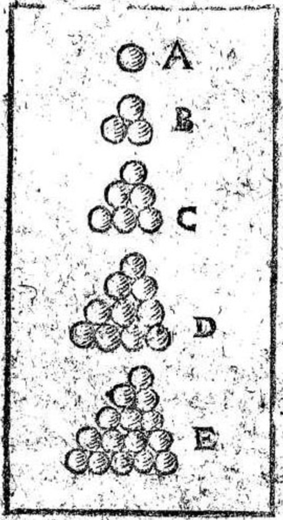
Figure 1.
Woodcut of
Kepler sphere
arrangements

The cannonball packing had been studied earlier by the English mathematician Thomas Hariot  [Harriot]  (1560–1621). Hariot was mathematics tutor to Sir Walter Raleigh, designed some of his ships, wrote a treatise on navigation, and went on an expedition to Virginia in 1585–1587 as surveyor, reporting on it in 1590 in  [53], his only published book. He computed a chart in 1591 on how to most efficiently stack cannonballs using the $\operatorname{FCC}$ packing, and computed a table of the number of cannonballs in such stacks (see Shirley  [91, pp. 242–243]). Hariot supported the atomic theory of matter, in which case macroscopic objects may be packed in arrangements of very tiny spherical objects, i.e. atoms  [60, Chap. III]. He corresponded with Kepler in 1606–1608 on optics, and mentioned the atomic theory in a December 1606 letter as a possible way of explaining why some light is reflected, and some refracted, at the surface of a liquid. Kepler replied in 1607, not supporting the atomic theory. The known correspondence of Hariot with Kepler does not deal directly with sphere packing.

The statement that the maximal density of a sphere packing in $3$-dimensional space equals $\frac{\pi}{\sqrt{18}}\approx 0.74048$, which is attained by the $\operatorname{FCC}$ packing, is called the Kepler Conjecture. It was settled affirmatively in the period 1998–2004 by Hales with Ferguson  [65]. A second generation proof, which is a formal proof checked entirely by computer, was recently completed in a project led by Hales  [51].

2.2. Newton and Gregory (1694)

In 1694 Isaac Newton (1642–1727) and David Gregory (1659?- 1708) had a discussion of touching spheres related to preparing a second edition of Newton’s Principia. It concerned the question whether the “fixed stars” are subject to gravitational attraction. What force is “balancing” their apparent fixed positions?

Gregory  [80, Vol III, p. 317] summarized in a memorandum a conversation with Newton on 4 May 1694 concerning the brightest stars as:

To discover how many stars there are of a given magnitude, he [Newton] considers how many spheres, nearest, second from them, third etc. surround a sphere in a space of three dimensions, there will be $13$ of first magnitude, $4\times 13$ of second, $9\times 4\times 13$ of third.

Newton’s own star table “A Table of ye fixed Starrs for ye yeare 1671” records $13$ first magnitude stars, $43$ of the second magnitude, $174$ of third magnitude (see  [80, Vol  II,  p.  394]).

Newton drafted a new Proposition to be included in a second edition of the Principia, stating [59, p. 81, in translation]:

Proposition XV. Theorem XV. The fixed stars are at rest in the heavens and are separated by enormous distances from our Sun and from each other.

In a draft proof he wrote [59, p. 85, in translation]:

That the stars are at huge distances from our Sun is clear enough from the absence of parallax; and that they lie at no less distances from each other may be inferred from their differing apparent magnitudes. For there are $13$ stars of the first magnitude and roughly the same number of equal spheres can be arranged about a central sphere equal to them.

and:

For if around some sphere there are arranged more spheres of about the same size, the number of spheres which surround it closely will be $12$ or $13$; at the second stage about $50$; at the third about $110$ [roughly $9\times 12$]; at the fourth, $200$ [$16\times 12\frac{1}{2}$], …

This argument is similar to one of Kepler  [62, Liber I, Pars II, p. 138] (translation in Koyré  [63, p. 80]), with roots in the claim of Giordano Bruno, that all stars are suns.

After further work, through several drafts, Newton abandoned this Proposition (according to Hoskin  [59]). It was not included in the second edition of the Principia, when it was later published in 1713.

Gregory continued study of the geometric problem underlying the spacing of stars. In an (unpublished) notebook he considered the packing problem of $2$-dimensional disks in concentric rings and, in $3$ dimensions, that of equal spheres, noting that $13$ spheres might touch a given equal sphere  [80, Vol III, Letter 441, Note (10), p. 321]. He considered the $13$ sphere question in later years, making the following memorandum in 1704 [56, p. 21]:

Oxon. 23 Nov^r 1704. Mr. Kyl said that if $13$ equal spheres touch an equal inmost sphere, $9\times 13$ must touch one that include these former $14$, because there is nine times as much surface to stand on. I told him that we must reckon by the surface passing through their centers.

A manuscript of Gregory on Astronomy, translated into English and posthumously published in 1715, states [46, p. 289, sic]:

For if every Fix’d Star did the office of a Sun, to a portion of the Mundane space nearly equal to this that our Sun commands, there will be as many Fix’d Stars of the first Magnitude, as there can be Systems of this sort touching and surrounding ours; that is, as many equal Spheres as can touch an equal one in the middle of them. Now, ’tis certain from Geometry, that thirteen Spheres can touch and surround one in the middle equal to them, (for Kepler is wrong in asserting, in B. I of the Epit. that there may be twelve such, according to the number of Angles of an Icosaedrum,)

Thus Gregory expressed a definite opinion that $13$ spheres might touch.

2.3. Bender, Hoppe, Günther (1874)

The issue of whether $13$ equal spheres might touch a central equal sphere was discussed in the physics literature in the period 1874–1875, with contributions by C. Bender  [10], Reinhold Hoppe  [58] and Siegmund Günther  [47]. Hoppe noted a mathematical gap in the argument of Bender. Günther offered a physical intuition, but no proof. They all concluded that at most $12$ unit spheres could touch a central unit sphere. In 1994 Hales  [49] noted a mathematical gap in the argument of Hoppe.

2.4. Barlow (1883)

In another context the crystallographer William Barlow (1845–1934) noted another optimal sphere packing, the Hexagonal Close Packing ($\operatorname{HCP}$). In a paper “Probable nature of the internal symmetry of crystals”  [8, p. 186] he considered five symmetry types for crystal structure. The third kind of symmetry he describes is the $\operatorname{FCC}$ packing (Fig. 4 and 4a). He then stated:

A fourth kind of symmetry, which resembles the third in that each point is equidistant from the twelve nearest points, but which is of a widely different character than the three former kinds, is depicted if layers of spheres in contact arranged in the triangular pattern (plan d) are so placed that the sphere centers of the third layer are over those of the first, those of the fourth layer over those of the second, and so on. The symmetry produced is hexagonal in structure and uniaxial (Figs. 5 and 5a).

Here “plan d” is the two-dimensional hexagonal packing, and Figs. 5 and 5a depict the $\operatorname{HCP}$ packing. He suggested that the atoms in a crystal of quartz ($SiO_{2}$) occur with the fourth kind of symmetry (see Figure  2).

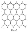
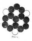
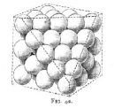
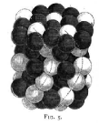
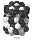
Figure 2. Barlow $\operatorname{FCC}$ and $\operatorname{HCP}$ packings

Barlow also stated later in the paper  [8, Figs. 7 and 8, p.207] the following about twinned crystal arrays with a connecting layer:

The peculiarities of crystal-grouping displayed in twin crystals can be shown to favour the supposition that we have in crystals symmetrical arrangement rather than symmetrical shape of atoms or small particles. Thus if an octahedron be cut in half by a plane parallel to two opposite faces, and the hexagonal faces of separation, while kept in contact and their centres coincident, are turned one upon the other through $60^{\circ}$, we know that we get a familiar example of a form found in some twin crystals. And a stack can be made of layers of spheres placed triangularly in contact to depict this form as readily as to depict a regular octahedron, the only modification necessary being for the layers above the centre layer to be placed as though turned bodily through $60^{\circ}$, from the position necessary to depict an octahedron (compare Figs. 7 and 8). The modification, as we see, involves no departure from the condition that each particle is equidistant from the twelve nearest particles.

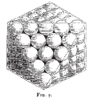
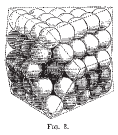
Figure 3. Barlow Twinned Crystal Packing

2.5. Tammes (1930)

The Dutch botanist Pieter Merkus Lambertus Tammes made in 1930 a study of the equidistribution of pores on pollen grains  [92]. He asked the question: What is the maximum number of circular caps $N(\theta)$ of angular diameter $\theta$ that can be placed without overlap on a unit sphere? Here $\theta$ is measured from the center of the unit sphere $\SS^{2}$ in $\mathbb{R}^{3}$. Tammes  [92, Chap. 3] empirically determined that $N(\frac{\pi}{2})=6$, while $N(\theta)\leq 4$ for $\theta>\frac{\pi}{2}$. Let $\theta=\theta(N)$ denote the maximal value of $\theta$ having $N(\theta)=N$. He concluded that $\theta(5)=\theta(6)=\frac{\pi}{2}$.

The problem of determining various values of $N(\theta)$ is now called the Tammes problem. It is related to a dual question of determining the maximal radius $r(N)$ possible for $N$ equal spheres all touching a central sphere of radius $1$. Namely, the maximal value of $\theta:=\theta(N)$ having $N(\theta)=N$, determines the maximal allowable radius $r(N)$ of $N$ spheres touching a central unit sphere by a formula given in Lemma  3.1 below.

2.6. Fejes Tóth (1943)

In 1943 László Fejes Tóth  [34] conjectured that the volume of any Voronoi cell of any sphere packing of ${\mathbb{R}}^{3}$ by unit spheres is minimized by the dodecahedral configuration of $12$ unit spheres touching a central sphere. The Voronoi cell of the central sphere is then a regular dodecahedron circumscribed about the sphere. The packing density of the dodecahedron is approximately $0.7546$, which is larger than the density of the known FCC packing of ${\mathbb{R}}^{3}$. This conjecture became known as the Dodecahedral Conjecture and was settled affirmatively in 2010 (see Section  5.4).

2.7. Frank (1952)

The problem of molecular rearrangement in the liquid-solid phase transition is relevant in materials. The structure of ordinary ice, the $H_{2}O$ phase labeled ice $I_{h}$, has an $\operatorname{HCP}$ packing of its oxygen atoms, as observed in 1921 by Dennison  [24]. Note that the hydrogen atoms are free to change their orientations to some extent (Pauling  [81]). Water exhibits a phenomenon of supercooling at standard pressure down to $-48^{\circ}C$; under special rapid cooling it can avoid freezing down to $-137^{\circ}C$, and enter a glassy phase (Angell  [5]).

In 1952 Frederick Charles Frank  [40] argued that supercooling can occur because the common arrangements of molecules in liquids assume configurations far from what they would assume if frozen. He wrote:

Consider the question of how many different ways one can put twelve billiard balls in simultaneous contact with another one, counting as different the arrangements which cannot be transformed into each other without breaking contact with the centre ball?’ The answer is three. Two which come to the mind of any crystallographer occur in the face-centred cubic and hexagonal close packed lattices. The third comes to the mind of any good schoolboy, and it is to put one at the centre of each face of a regular dodecahedron. That body has five-fold axes, which are abhorrent to crystal symmetry: unlike the other two packings, this one cannot be continuously extended in three dimensions. You will find that the outer twelve in this packing do not touch each other. If we have mutually interacting deformable spheres, like atoms, they will be a little closer to the centre in this third kind of packing; and if one assumes they are argon atoms (interacting in pairs with attractive and repulsive potentials proportional to $r^{-6}$ and $r^{-12}$) one may calculate that the binding energy of the group of thirteen is $8.4\%$ greater than for the other two packings. This is $40\%$ of the lattice energy per atom in the crystal. I infer that this will be a very common grouping in liquids, that most of the groups of twelve atoms around one will be of this form, that freezing involves a substantial rearrangement, and not merely an extension of the same kind of order from short distances to long ones; a rearrangement which is quite costly of energy in small localities, and which only becomes economical when extended over a considerable volume, because unlike the other packing it can be so extended without discontinuities.

The three local arrangements Frank specifies we shall label as $\operatorname{FCC}$ (face-centered-cubic), $\operatorname{HCP}$ (hexagonal close packing) and $\operatorname{DOD}$ (dodecahedral), for convenience. The crystalline arrangements of $\operatorname{FCC}$ and $\operatorname{HCP}$ are “extremal” (i.e. on the boundary of the configuration space), while the balls in $\operatorname{DOD}$ configuration are free to move independently.

Frank’s assertion that there are exactly three possible arrangements is false if taken literally. There are continuous deformations between any arrangement of types $\operatorname{FCC}$, $\operatorname{HCP}$ and $\operatorname{DOD}$ and any of the other types (see Section  5.4). There is however an important kernel of truth in Frank’s statement, which buttresses his argument made concerning the existence of supercooling: each of the three arrangements above is “remarkable” in some sense (see Section  5). To move from a large arrangement of spheres having many $\operatorname{DOD}$ configurations to one frozen in the $\operatorname{HCP}$ packing requires substantial motion of the spheres.

2.8. Schütte and van der Waerden (1953)

In a paper titled “Das Problem der dreizehn Kugeln” [“The problem of the thirteen balls”] Kurt Schütte and Bartel Leendert van der Waerden  [88] gave a rigorous proof that one cannot have $13$ unit spheres touching a given central sphere.

There has been much further work on this problem. In his 1956 paper titled “The problem of $13$ spheres” John Leech  [66] gave a two page proof of the impossibility of $13$ unit spheres touching a unit sphere. More accurately he stated: “In the present paper I outline an independent proof of this impossibility, certain details which are tedious rather than difficult have been omitted.” Various authors have written to fill in such details, which balloon the length of the proof. These include work of Maehara  [71] in 2001, who gave in 2007 a simplified proof  [72]. Other proofs of the thirteen spheres problem were given by Anstreicher  [4] in 2004 and Musin  [75] in 2006.

2.9. Fejes Tóth (1969)

In 1969 László Fejes Tóth  [39] discussed the problem of characterizing those sphere packings in space that have the property that every sphere in the packing touches exactly $12$ neighboring spheres. The $\operatorname{FCC}$ and $\operatorname{HCP}$ packing both have this property, as already noted by Barlow (1883). There are in addition uncountably many other packings, obtained by stacking plane layers of hexagonally packed spheres (“penny packing”), where there are two choices at each level of how to pack the next level. Fejes Tóth conjectured that all such packings are obtained in this way.

This conjecture of Fejes Tóth’s was settled affirmatively by Hales  [50] in 2013.

2.10. Conway and Sloane (1988)

In their book: Sphere Packings, Lattices and Groups, John H. Conway and Neil J. A. Sloane considered the question: What rearrangements of the $12$ unit spheres are possible using motions that maintain contact with the central unit sphere at all times? In  [20, Chap. 1, Appendix: Planetary Perturbations] they sketch a result asserting: The configuration space of $12$ unit spheres touching a $13$-th allows arbitrary permutations of all $12$ touching spheres in the configuration. That is, if the spheres are labeled and in the DOD configuration, it is possible, by moving them on the surface of the central sphere, to arbitrarily permute the spheres in a DOD configuration.

We will describe the motions in detail to obtain such permutations in Section  6.

3. Maximal Radius Configurations of $N$ Spheres: The Tammes Problem

What is the maximal radius $r(N)$ possible for $N$ equal spheres all touching a central sphere of radius $1$? This problem is closely related to the Tammes problem discussed above, which concerns instead the maximum number of circular caps $N(\theta)$ of angular diameter $\theta$ that can be placed without overlap on a sphere. The latter problem is also the problem of constructing good spherical codes (see  [20, Chap. 1, Sec. 2.3]).

3.1. Radius versus Angular Diameter Parameterization

One can convert the angular measure $\theta$ into the radius of touching spheres; for a sphere touching a central unit sphere, its associated spherical cap on the central sphere is the radial projection of its points onto the surface of the central sphere.

Figure 4. Angular measure $\theta$ related to radius $r$

Lemma 3.1.

For a fixed $N>2$, the maximal value of  $\theta:=\theta_{max}(N)$ having $N(\theta)=N$ determines the maximal allowable radius $r_{max}(N)$ of $N$ spheres touching a central unit sphere, using the formula

$$r_{max}(N)=\frac{\sin\mathopen{}\mathclose{{}\left(\frac{\theta(N)}{2}}\right)}{1-\sin\mathopen{}\mathclose{{}\left(\frac{\theta(N)}{2}}\right)}.$$

Conversely, given $r=r_{max}(N)$, we obtain

$$\theta_{max}(N)=2\arcsin\mathopen{}\mathclose{{}\left(\frac{r}{1+r}}\right),$$

choosing $0<\theta(N)<\pi$.

Proof.

From the right triangle in Figure  4 we have

$$\sin\frac{\theta}{2}=\frac{r}{1+r}.$$

This relation gives a bijection of the interval $0\leq\theta<\pi$ to the interval $0\leq r<\infty.$ ∎

3.2. Rigorous Results for Small $N$

The Tammes problem has been solved exactly for only a few values of $N$, including $3\leq N\leq 14$ and $N=24$.

3.2.1. Fejes Tóth: ​​$N\!\!=\!3,4,6,12$

The Tammes problem was solved for $N\!\!=\!3,4,6$ and $12$ by László Fejes Tóth  [33] in 1943, where extremal configurations of touching points for $N\!=3$ are attained by vertices of an equilateral triangle arranged around the equator, and for $N\!\!=\!4,6,12$ by vertices of regular polyhedra (tetrahedron, octahedron and icosahedron) inscribed in the unit sphere. Fejes Tóth proved the following inequality: For $N$ points on the surface of the unit sphere, at least two points can always be found with spherical distance

$$d\leq\arccos\Big{(}\frac{(\cot\omega)^{2}-1}{2}\Big{)},\quad\mbox{with}\quad\omega=\Big{(}\frac{N}{N-2}\Big{)}\frac{\pi}{6}.$$

Note that $d$ is the edge-length of a spherical equilateral triangle with the expected area for an element of an $N$-vertex triangulation of $\SS^{2}$. The inequality is sharp for $N\!=3,4,6$ and $12$ for the specified configurations above.

In 1949 Fejes Tóth  [35] gave another proof of his inequality. His result was re-proved by Habicht and van der Waerden  [48] in 1951. After converting this result to the $r$-parameter using Lemma  3.1, we may re-state his result for $N=12$ as follows.

Theorem 3.2.

(Fejes Tóth (1943))

$(1)$ The maximum radius of $12$ equal spheres touching a central sphere of radius $1$ is:

$$r_{max}(12)=\frac{1}{\sqrt{\frac{5+\sqrt{5}}{2}}-1}\approx 1.1085085.$$

Here $r_{max}(12)$ is a real root of the fourth degree equation $x^{4}-6x^{3}+x^{2}+4x+1=0$.

$(2)$ An extremal configuration achieving this radius is the $12$ vertices of an inscribed regular icosahedron (equivalently, face-centers of a circumscribed regular dodecahedron).

3.2.2. Schütte and van der Waerden: $N=5,7,8,9$

The Tammes problem was solved for $N=5$ in 1950 by van der Waerden, building on work of Habicht and van der Waerden  [48]. It was solved for $N=7$ by Schütte. These solutions, plus those of van der Waerden for $N=8$ and Schütte for $N=9$ appear in Schütte and van der Waerden  [87]. They give a history of these developments in  [87, p. 97].

Their paper used geometric methods, introducing and studying the allowed structure of the graphs describing the touching patterns of arrangements of $N$ equal circles on $\SS^{2}$. These graphs are now called contact graphs, and Schütte and van der Waerden credit their introduction to Habicht. Schütte also conjectured candidates for optimal configurations for $N=10,13,14,15,16$ and van der Waerden conjectured candidates for $N=11,24,32$ (see  [87]).

L. Fejes Tóth presented the work of Schütte and van der Waerden in his 1953 book on sphere-packing  [36, Chapter VI]. This book uses the terminology of maximal graph for the graph of a configuration achieving the maximal radius for $N$. In 1959 Fejes Tóth  [37] noted that the set of vertices of a square antiprism gave an extremal $N=8$ configuration on the $2$-sphere.

3.2.3. Danzer: $N=6,7,8,9,10,11$

In his 1963 Habilitationsschrift  [22] (see the 1986 English translation  [23]), Ludwig Danzer made a geometric study of the contact graph for a configuration of $N$ circles on the surface of a sphere. This graph has a vertex for each circle and an edge for each pair of touching circles. A contact graph is called maximal if it occurs for a set of circles achieving the maximal radius $r_{max}(N)$. It is called optimal if it has the minimum number of edges among all maximal contact graphs. A contact graph is called irreducible if the radius cannot be improved by altering a single vertex. For each small $N$, Danzer found a complete list of irreducible contact graphs. He used this analysis to prove the conjectures of Schütte and van der Waerden  [87] above for the cases $N=10,11$.

Theorem 3.3.

(Danzer (1963))

$(1)$ For $7\leq N\leq 12$ there is, up to isometry, a unique $\theta$-maximizing unlabeled configuration of spheres with $N(\theta)=N$.

$(2)$ For $N=12$, the vertices of a regular icosahedron form the unique $\theta$-maximizing configuration. The $\theta$-maximizing configuration for $N=11$ is a regular icosahedron with one vertex removed.

In  [23, Theorem II] Danzer classified irreducible sets for $72^{\circ}=\frac{2\pi}{5}<\theta<90^{\circ}=\frac{2\pi}{4}$. There are additional $N$-irreducible graphs for $N=7,8,9,10$ in these cases. For $N=6,7,8,9$ he finds one optimal set and one irreducible set with one degree of freedom. He also finds for $N=8$ an irreducible set with two degrees of freedom. For $N=10$ he finds one optimal set, two irreducible sets with no degrees of freedom, and five with at least one degree of freedom. Danzer states that the irreducible sets with no degrees of freedom (presumably) give relative optima. An irreducible graph having a degree of freedom fails to be relatively optimal, since deforming along its degree of freedom leads to a boundary graph with an additional edge, where the extrema is reached.

Danzer’s work was not published in a journal until the 1980’s. In the interm, Böröczky  [11] gave another solution for $N=11$, and Hárs  [54] for $N=10$.

3.2.4. Musin and Tarasov: $N=13,14$

Very recently the Tammes problem was solved for the cases $N=13$ and $N=14$ by Oleg Musin and Alexey Tarasov  [76, 78]. Their proofs were computer-assisted, and made use of an enumeration of all irreducible configuration contact graphs (see  [77]). Earlier work on configurations of up to $17$ points was done by Böröczky and Szabó  [12, 13]).

3.2.5. Robinson: $N=24$

The case $N=24$ was solved in 1961 by Raphael M. Robinson  [85]. He proved a 1959 conjecture of Fejes Tóth  [38], asserting that the extremal $\theta(24)~{}\approx~{}43^{\circ}\,\,42^{{}^{\prime}}$ and that the extremal configuration of $24$ sphere centers are the vertices of a snub cube. Coxeter  [21, p. 326] describes the snub cube.

3.3. The Tammes Problem: Optimal Contact Graphs and Optimal Parameters

Table  1 summarizes optimal angular parameters and radius parameters on the Tammes problem for $3\leq N\leq 14$ and $N=24$ (see Aste and Weaire  [7, Sect. 11.6]). The configuration name given is associated to the vertices in the corresponding polyhedron being inscribed in a sphere, e.g. an icosahedron has $N=12$ vertices (see Melnyk et al.  [73, Table 2]). In the case $N=5$ the polyhedron is any from a family of trigonal bipyramids, including the square pyramid as a degenerate case. For $N=11$ the polyhedron is a singly capped pentagonal antiprism, i.e. the icosahedron with one vertex deleted. The cases $N=7,9$ and $10$ are described in  [73, pp. 1747–1749]. Figure  5 shows schematically the optimal contact graphs for $3\leq N\leq 14$.

$N$	$\theta_{max}(N)$	$r_{max}(N)$	Configuration	Source
3	$\frac{2\pi}{3}=120^{\circ}$	$3+2\sqrt{3}$ $\approx 6.4641$	Equilateral Triangle	Fejes Tóth (1943)
4	$\cos^{-1}(-\frac{1}{3})$           $\approx 109.4712^{\circ}$	$2+\sqrt{6}$ $\approx 4.4495$	Regular Tetrahedron	Fejes Tóth (1943)
5	$\frac{2\pi}{4}=90^{\circ}$	$1+\sqrt{2}$ $\approx 2.4142$	Triangular Bipyramid	Fejes Tóth (1943)
6	$\frac{2\pi}{4}=90^{\circ}$	$1+\sqrt{2}$ $\approx 2.4142$	Regular Octahedron	Fejes Tóth (1943)
7	$\approx 77.8695^{\circ}$	$\approx 1.6913$	[No name]	Schutte and van der Waerden (1951)
8	$\approx 74.8585^{\circ}$	$\approx 1.5496$	Square Antiprism	Schutte and van der Waerden (1951)
9	$\approx 70.5288^{\circ}$	$\frac{1+\sqrt{3}}{2}$ $\approx 1.3660$	[No name]	Schutte and van der Waerden (1951)
10	$\approx 66.1468^{\circ}$	$\approx 1.2013$	[No name]	Danzer (1963)
11	$\approx 63.4349^{\circ}$	$\frac{1}{\sqrt{\frac{5+\sqrt{5}}{2}}-1}$ $\approx 1.1085$	Regular Icosahedron minus one vertex	Danzer (1963)
12	$\approx 63.4349^{\circ}$	$\frac{1}{\sqrt{\frac{5+\sqrt{5}}{2}}-1}$ $\approx 1.1085$	Regular Icosahedron	Fejes Tóth (1943)
13	$\approx 57.1367^{\circ}$	$\approx 0.9165$	[No name]	Musin and Tarasov (2013)
14	$\approx 55.6706^{\circ}$	$\approx 0.8759$	[No name]	Musin and Tarasov (2015)
24	$\approx 43.6908^{\circ}$	$\approx 0.5926$	Snub Cube	Robinson (1961)

Table 1. The Tammes Problem for small $N$

$N=3$

$N=4$

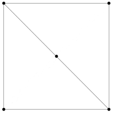
$N=5$

$N=6$

$N=7$

$N=8$

$N=9$

$N=10$

$N=11$

$N=12$

$N=13$

$N=14$

Figure 5. Optimal contact graphs associated to the Tammes configurations
for $N=3$ to $N=14$

3.4. The Tammes Problem Maximal Radius: General $N$

The most basic question about the maximal radius in the Tammes problem concerns the distinctness of maximal values. The following conjecture was proposed by R. M. Robinson  [86, p. 297].

Conjecture 3.4.

(Robinson (1969)) For all $N\geq 4$ the maximal radius satisfies

$$r_{max}(N)<r_{max}(N-1)$$

except possibly for $N=6,12,24,48,60$ and $120$.

One has $r_{max}(N)=r_{max}(N-1)$ for $N=6$ and $N=12$ by results already given above. In 1991 Tarnai and Gáspár  [94] established that $r_{max}(24)<r_{max}(23)$. The remaining cases $N\!\!=\!48$, $60$ and $120$ are open, but since strict inequality holds for $n=24$ we expect strict inequality to hold for these values too. However up to now it has been computationally difficult to determine $r_{max}(N)$ for such large $N$.

We turn to a potentially easier question. The known exact values of $r_{max}(N)$ are algebraic numbers, i.e. roots of some univariate polynomial having integer coefficients. Table  2 below presents algebraicity data for $3\leq N\leq 14$.

$N$	$r_{max}(N)$	Minimal Equation	Figure
3	$3+2\sqrt{3}$	$X^{2}-6X-3$	Equilateral Triangle
	$\approx 6.4641$
4	$2+\sqrt{6}$	$X^{2}-4X-2$	Regular Tetrahedron
	$\approx 4.4495$
6	$1+\sqrt{2}$	$X^{2}-2X-1$	Regular Octahedron
	$\approx 2.4142$
7	$\approx 1.6913$	$X^{6}-6X^{5}-3X^{4}$	[No name]
		$+8X^{3}+12X^{2}+6X+1$
8	$\approx 1.5496$	$X^{4}-8X^{3}+4X^{2}+8X+2$	Square Antiprism
9	$\approx 1.3660$	$2X^{2}-2X-1$	[No name]
10	$\approx 1.2013$	$4X^{6}-30X^{5}+17X^{4}$	[No name]
		$+24X^{3}-4X^{2}-6X-1$
12	$\frac{1}{\sqrt{\frac{5+\sqrt{5}}{2}}-1}$	$X^{4}-6X^{3}+X^{2}+4X+1$	Regular Icosahedron
	$\approx 1.10851$
24	$\approx 0.59262$	$X^{6}-10X^{5}+23X^{4}$	Snub Cube
		$+20X^{3}-5X^{2}-6X-1$

Table 2. The Tammes Problem radii given as algebraic numbers

We ask: Is the optimal radius $r_{max}(N)$ an algebraic number for each $N\geq 3$? The reason to expect such an algebraicity result to hold is that such a radius should be specified by at least one optimal graph that is rigid, i.e. it permits no local deformations preserving optimality, up to isometry. Danzer showed rigidity to be the case for $7\leq N\leq 12$. The equal length constraints of the edges of the contact graph give a system of polynomial equations with integer coefficients that the coordinates of the sphere centers must satisfy. One may expect that its real solution locus will include some real algebraic solutions for the sphere centers, leading to algebraicity of the radius. Even if the rigidity result fails and deformations occur (as happens for $N=5$), it could still be the case that the optimal radius is algebraic.

4. Configuration Spaces of $N$ Spheres Touching a Central Sphere

We start with the classical configuration space $\operatorname{Conf}(N):=\operatorname{Conf}(\SS^{2},N)$ of $N$ distinct labeled points on the unit $2$-sphere $\SS^{2}$. One may regard these as the points where $N$ surrounding spheres touch a central sphere. Note that $\operatorname{Conf}(N)$ is an open submanifold of the $N$-fold product $(\SS^{2})^{N}$ of unit spheres. We will also consider the reduced configuration space

$$\operatorname{BConf}(N):=\operatorname{Conf}(N)/SO(3),$$

which divides out the space $\operatorname{Conf}(N)$ by the orientation-preserving isometry group $SO(3)$ of the unit $2$-sphere $\SS^{2}$ in ${\mathbb{R}}^{3}$. The elements of $SO(3)$ move all configurations to isometric configurations, and these moves are permitted on any configuration. The space $\operatorname{Conf}(N)$ is a non-compact $(2N)$-dimensional manifold and the space $\operatorname{BConf}(N)$ is a non-compact $(2N-3)$-dimensional manifold. We assume $N\geq 3$ to avoid degenerate cases.

We denote a configuration ${\bf U}:=({\bf u}_{1},{\bf u}_{2},...,{\bf u}_{N})$, where the ${\bf u}_{j}\in\SS^{2}$ are distinct points. The angular distance between points ${\bf u}_{1},{\bf u}_{2}\in\SS^{2}$ is the angle ${\bf u}_{1},0,{\bf u}_{2}$ subtended at the center of the unit sphere that the $N$ spheres all touch; its value is at most $\pi$.

Definition 4.1.

The injectivity radius function $\rho:\,\operatorname{Conf}(\SS^{2},N)\to{\mathbb{R}}_{+}$ assigns to a configuration ${\bf U}:=({\bf u}_{1},{\bf u}_{2},\dots,{\bf u}_{N})\in(\SS^{2})^{N}$ the value

$$\rho({\bf U}):=\frac{1}{2}\big{(}\min_{i\neq j}\theta({\bf u}_{i},{\bf u}_{j})\big{)},$$

where $\theta({\bf u}_{i},{\bf u}_{j})$ denotes the angular distance between ${\bf u}_{i}$ and ${\bf u}_{j}$. In particular $0<\rho({\bf U})\leq\frac{\pi}{2}.$ Since the function $\rho$ is invariant under the action of $SO(3)$, it yields a well-defined function on $\operatorname{BConf}(N;\theta)$, which we also denote $\rho$.

Our main topic in this section is the study of spaces which are superlevel sets for the injectivity radius function $\rho$, and how these change at configurations which are critical for maximizing $\rho$.

Definition 4.2.

We define the (constrained) angular configuration spaces

$$\operatorname{Conf}(N;\theta)=\operatorname{Conf}(\SS^{2},N;\theta):=\{{\bf U}=({\bf u}_{1},...,{\bf u}_{N}):\,\theta({\bf u}_{i},{\bf u}_{j})\geq\theta\,\,\mbox{for}\,\,1\leq i<j\leq N\}$$

for angles $0<\theta\leq\pi$, whose points label configurations of $N$ distinct marked labeled points ${\bf u}_{i}$ which are pairwise at angular distance at least $\theta$ from each other. Equivalently

$$\operatorname{Conf}(N;\theta):=\{{\bf U}=({\bf u}_{1},...,{\bf u}_{N}):\,\rho({\bf U})\geq\frac{\theta}{2}\}.$$

The reduced (constrained) angular configuration spaces $\operatorname{BConf}(N;\theta)$ are

$$\operatorname{BConf}(N;\theta):=\operatorname{Conf}(N;\theta)/SO(3).$$

This space is well-defined since rotations preserve angular distance.

The spaces $\operatorname{Conf}(N;\theta)$ and $\operatorname{BConf}(N;\theta)$ are compact topological spaces. Away from critical values $\theta$ the spaces $\operatorname{Conf}(N;\theta)$ are closed manifolds with boundary; at critical points they need not be manifolds. The descriptions as superlevel sets show that the spaces $\operatorname{Conf}(N;\theta)$ are ordered by set inclusion as decreasing functions of $\theta$. If $\theta_{1}>\theta_{2}$ then we have

$$\operatorname{Conf}(N;\theta_{1})\subset\operatorname{Conf}(N;\theta_{2})\subset\operatorname{Conf}(N).$$

We have similar inclusions for $\operatorname{BConf}(N;\theta)$. The interiors of these spaces are

$$\operatorname{Conf}^{+}(N;\theta):=\{{\bf U}=({\bf u}_{1},...,{\bf u}_{N}):\,\rho({\bf U})>\frac{\theta}{2}\}$$

and

$$\operatorname{BConf}^{+}(N;\theta):=\operatorname{Conf}^{+}(N;\theta)/SO(3),$$

respectively. They are open manifolds for all values of the parameter $\theta$.

The (constrained) angular configuration space $\operatorname{Conf}(N;\theta)$ can be reparametrized as the (constrained) radial configuration space

$$\operatorname{Conf}(N)[r]:=\operatorname{Conf}(\SS^{2},N)[r]$$

which consists of $N$ marked labeled spheres of equal radius $r=r(\theta)$ in ${\mathbb{R}}^{3}$ which all touch a given unit radius central sphere $\SS^{2}$, with the $N$ touching points being the labeled points of the configuration. The radius $r(\theta)$ is determined by the condition that the spherical cap on the central sphere $\SS^{2}$ obtained by radial projection of all the points of the given touching sphere has angular diameter exactly $\theta$. A configuration belongs to $\operatorname{Conf}(N;\theta)$ exactly when the $N$ spheres of radius $r(\theta)$ have disjoint interiors. There is a maximal angle $\theta_{max}:=\theta_{max}(N)$ for which $N$ spherical caps of that angular measure can fit on the surface of $\SS^{2}$ without overlap of their interiors.

Recall from the proof of Lemma  3.1 that the value $r=r(\theta)$ is implicitly given by the equation

$$\sin\frac{\theta}{2}=\frac{r}{1+r}.$$

For $N\geq 3$ the function $r(\theta)$ is monotone increasing in $\theta$ up to a maximal value $r_{max}(\theta)$, so we may use either $r$ or $\theta$ to parametrize the family of all spaces $\operatorname{Conf}(N;\theta)$ or $\operatorname{Conf}(N)[r]$. Note that we can identify the configuration spaces $\operatorname{Conf}(N)$ with $\operatorname{Conf}(N;0)$, as well as with $\cup_{\theta>0}\operatorname{Conf}(N;\theta)$ and $\cup_{r>0}\operatorname{Conf}(N)[r]$.

In the following subsections we review the topology and geometry of the spaces $\operatorname{Conf}(N;\theta)$ and $\operatorname{BConf}(N;\theta)$:

• In Section  4.1 we describe results on the homotopy type and cohomology of the configuration spaces $\operatorname{Conf}(N)$ and reduced configuration spaces $\operatorname{BConf}(N)$, which are well studied.

• In Section  4.2 we use ideas from Morse theory, applied to the injectivity radius function $\rho$, to study general features of the change in topology for fixed $N$ as the angular parameter $\theta$ (or radius parameter $r$) is increased. The topology changes at certain critical values of $\theta$. Since the injectivity radius function $\rho$ is semi-algebraic, for each $N$ we expect there to be a finite set of critical values of $\rho$ on $\operatorname{BConf}(N)$. We give a balancing criterion for a configuration in $\operatorname{BConf}(N)$ to be critical.

• In Section  4.3 we show that for small enough $\theta$, the angular configuration space $\operatorname{Conf}(N;\theta)$ has the same homotopy type as $\operatorname{Conf}(N)$ and hence the same cohomology.

• In Section  4.4 we treat large $\theta$ near $\theta_{max}$, in terms of the radius parameter $r$. For larger angular diameter $\theta$, the topology of $\operatorname{Conf}(N;\theta)$ may differ drastically from that of $\operatorname{Conf}(N)$. For example, in Table  1 for the Tammes problem many of the maximal configurations are isolated, and the associated labeled spheres cannot be continuously interchanged for large $\theta$ near $\theta_{max}(N)$. In such situations, the space $\operatorname{Conf}(N;\theta)$ is disconnected for large $\theta$, while the space $\operatorname{Conf}(N)$ is connected. We conjecture that near $\theta_{max}(N)$ the cohomology of $\operatorname{BConf}(N)[r]$ is concentrated in dimension $0$ and discuss the associated Betti number.

• In Section  4.5 we show by examples that the set of critical configurations at a critical value can have many connected components and can have variable dimension.

• In Section  4.6 we treat the case of topology change as $\theta$ varies for the simplest case $N=4$. We determine all the critical values for the injectivity radius function $\rho$ on $\operatorname{BConf}(N)$.

• In Section  4.7 we briefly discuss topology change in cases $N\geq 5$. The study of properties of the $N=12$ case is deferred to Sections  5 and  6.

4.1. Topology of Configuration Spaces

Configuration spaces $\operatorname{Conf}({\mathbb{X}},N)$ of $N$ distinct, labeled points on a $d$-dimensional manifold ${\mathbb{X}}$ have been studied as fundamental spaces in topology. Recall that the configuration space of labeled $N$-tuples on a manifold ${\mathbb{X}}$ is

$$\operatorname{Conf}({\mathbb{X}},N):=\{(x_{1},x_{2},...,x_{N})\in{\mathbb{X}}^{N}:\,x_{i}\neq x_{j}\,\textrm{{\mbox{i}f}}\,\,i\neq j\}.$$

The symmetric group $\Sigma_{N}$ acts freely on the space $\operatorname{Conf}({\mathbb{X}},N)$ to permute the points, and

$$B({\mathbb{X}},N):=\operatorname{Conf}({\mathbb{X}},N)/\Sigma_{N}$$

is the configuration space of unlabeled (i.e. unordered) $N$-tuples of points on ${\mathbb{X}}$. Configuration spaces of this type were first considered in the 1960’s by Fadell and Neuwirth  [30, 28]. The state of the art for ${\mathbb{X}}={\mathbb{R}}^{d}$ and $\SS^{d}$ as of 2000 is given in Fadell and Husseini  [29]. Other useful references are Totaro  [96] and Cohen  [17].

We begin with the most well-known of these spaces, the configuration space $\operatorname{Conf}({\mathbb{R}}^{2},N)$ of labeled $N$-tuples of points on ${\mathbb{X}}={\mathbb{R}}^{2}$, the plane. Fadell and Neuwirth  [30] showed that the unlabeled configuration space $B({\mathbb{R}}^{2},N)$ is a classifying space (Eilenberg-Maclane space  $K(\pi,1)$), with fundamental group $\pi_{1}=\pi$ isomorphic to Artin’s braid group $B_{N}$ on $N$ strings. Thus the cohomology of $B({\mathbb{R}}^{2},N)$ is just the cohomology of $B_{N}$; it was computed by Fuks  [41] and Cohen  [16].

The labeled configuration space $\operatorname{Conf}({\mathbb{R}}^{2},N)$ is by definition the complement of a finite set of complex hyperplanes given by $x_{i}=x_{j}$ for $i\neq j$ in ${\mathbb{C}}^{N}\cong({\mathbb{R}}^{2})^{N}$. This arrangement is sometimes called the (complexified) $A_{N-1}$-arrangement of hyperplanes (see Postnikov and Stanley  [84]), where $A_{N-1}$ refers to a Coxeter group. The space $\operatorname{Conf}({\mathbb{R}}^{2},N)$ is also a classifying space with fundamental group equal to the pure braid group $P\kern-1.99997ptB_{N}$, the subgroup of $B_{N}$ consisting of all $N$-strand braids which induce the identity permutation. It sits in a short exact sequence $0\to P\kern-1.99997ptB_{N}\to B_{N}\to\Sigma_{N}\to 0$. The rational cohomology of $\operatorname{Conf}({\mathbb{R}}^{2},N)$ is then the cohomology of the pure braid group; the cohomology ring structure of $P\kern-1.99997ptB_{N}$ was determined by Arnold  [6] in 1969.

The Betti numbers of a topological space are the ranks of its homology groups (which equal the ranks of its cohomology groups, with coefficients in a field, here ${\mathbb{Q}}$ or ${\mathbb{C}}$.) The generating function for this sequence of ranks is called the Poincaré polynomial. Arnold  [6, Corollary  2] determined the Poincaré polynomial for the pure braid group $P\kern-1.99997ptB_{N}$ on $N$ strands to be

$$P_{N}(t)=(1+t)(1+2t)\cdots(1+(N-1)t).$$ (4.1)

Table  3 gives these Betti numbers for small $N$. They are of combinatorial interest, being unsigned Stirling numbers of the first kind,

$$\dim H^{k}(P\kern-1.99997ptB_{N},{\mathbb{Q}})=\big{[}{{N}\atop{N-k}}\big{]},\quad\mbox{ for}\quad 0\leq k\leq N-1$$

(see  [45, Sect. 6.1]).

	$0$	$1$	$2$	$3$	$4$	$5$	$6$	$7$	$8$
$1$	$1$	$0$	$0$	$0$	$0$	$0$	$0$	$0$	$0$
$2$	$1$	$1$	$0$	$0$	$0$	$0$	$0$	$0$	$0$
$3$	$1$	$3$	$2$	$0$	$0$	$0$	$0$	$0$	$0$
$4$	$1$	$6$	$11$	$6$	$0$	$0$	$0$	$0$	$0$
$5$	$1$	$10$	$35$	$50$	$24$	$0$	$0$	$0$	$0$
$6$	$1$	$15$	$85$	$225$	$274$	$120$	$0$	$0$	$0$
$7$	$1$	$21$	$175$	$735$	$1624$	$1764$	$720$	$0$	$0$
$8$	$1$	$28$	$322$	$1960$	$6769$	$13132$	$13068$	$5040$	$0$
$9$	$1$	$36$	$546$	$4536$	$22449$	$67284$	$118124$	$109584$	$40320$

Table 3. Betti numbers of pure braid group cohomology
$H^{k}(P\kern-1.99997ptB_{N},{\mathbb{Q}})\cong H^{k}(\operatorname{BConf}({\mathbb{R}}^{2},N),{\mathbb{Q}})$

Our interest here is configuration spaces on

$${\mathbb{X}}=\SS^{2}=\{{\bf u}=(x,y,z):{\bf u}\cdot{\bf u}=x^{2}+y^{2}+z^{2}=1\},$$

the unit $2$-sphere embedded in ${\mathbb{R}}^{3}$. The configuration spaces of $\SS^{2}$ have a close relationship to those of ${\mathbb{R}}^{2}$, since $\SS^{2}$ is the one-point compactification of ${\mathbb{R}}^{2}$. Note also that $\SS^{2}$ is homeomorphic to $\mathbb{CP}^{1}$, the complex projective line. Tautologically the configuration space $\operatorname{Conf}(\SS^{2},1)\cong\SS^{2}$; and the space $\operatorname{Conf}(\SS^{2},2)$ is homeomorphic to an ${\mathbb{R}}^{2}$-bundle over $\SS^{2}$, hence homotopy equivalent to $\SS^{2}$ (see  [17, Example 2.4]). For $N\geq 3$ points we have a well-known result, given as follows in Feichtner and Ziegler  [32, Theorem 1].

Theorem 4.3.

For $N\geq 3$ the configuration space $\operatorname{Conf}(\SS^{2},N)$ of $N$ distinct labeled points on the $2$-sphere is the total space of a trivial $PSL(2,{\mathbb{C}})$-bundle over ${\mathcal{M}}_{0,N}$, the moduli space of conformal structures on the $N$-punctured complex projective line, modulo conformal automorphisms. Hence there is a homeomorphism

$$\operatorname{Conf}(\SS^{2},N)\cong PSL(2,{\mathbb{C}})\times{\mathcal{M}}_{0,N}.$$

Note that $PSL(2,{\mathbb{C}})$ is homotopy equivalent to its maximal compact subgroup $SO(3)$, the group of orientation preserving isometries of $\SS^{2}$.

The $SO(3)$-action on $\operatorname{Conf}(\SS^{2},N)$ permits us to rotate the first point to the north pole, from which we stereographically project the rest of the unit sphere to the plane ${\mathbb{R}}^{2}$. Since we are still free to rotate about the north pole, which corresponds to $SO(2)$ rotations in the plane, we can identify $\operatorname{Conf}({\mathbb{R}}^{2},N-1)/SO(2)$ with the reduced $N$-configuration space $\operatorname{BConf}(\SS^{2},N)$. The action of $SO(2)$ on $\operatorname{Conf}({\mathbb{R}}^{2},N-1)$ is free if $N\geq 3$, so we can regard $\operatorname{Conf}({\mathbb{R}}^{2},N-1)$ as a principal $SO(2)$-bundle over $\operatorname{BConf}(\SS^{2},N)$.

This principal bundle has a section, and thus is a product bundle, so the Poincaré polynomial $\tilde{P}_{N}(t)$ of the base $\operatorname{BConf}(\SS^{2},N)$ may be computed as the quotient of the well-known Poincaré polynomials $P(t)=P_{N-1}(t)=\big{(}1+t\big{)}\big{(}1+2t\big{)}\cdots\big{(}1+(N-2)t\big{)}$ for $\operatorname{Conf}({\mathbb{R}}^{2},N-1)$ from Equation (4.1) and $p(t)=(1+t)$ for $SO(2)$. It follows that $\operatorname{BConf}(\SS^{2},N)$ and $\mathcal{M}_{0,N}$ both have Poincaré polynomial

$$\tilde{P}_{N}(t)=P(t)/p(t)=\big{(}1+2t\big{)}\cdots\big{(}1+(N-2)t\big{)}.$$ (4.2)

We give the first few Betti numbers in the following table:

	$0$	$1$	$2$	$3$	$4$	$5$	$6$	$7$	$8$	$9$
$3$	$1$	$0$	$0$	$0$	$0$	$0$	$0$	$0$	$0$	$0$
$4$	$1$	$2$	$0$	$0$	$0$	$0$	$0$	$0$	$0$	$0$
$5$	$1$	$5$	$6$	$0$	$0$	$0$	$0$	$0$	$0$	$0$
$6$	$1$	$9$	$26$	$24$	$0$	$0$	$0$	$0$	$0$	$0$
$7$	$1$	$14$	$71$	$154$	$120$	$0$	$0$	$0$	$0$	$0$
$8$	$1$	$20$	$155$	$580$	$1044$	$720$	$0$	$0$	$0$	$0$
$9$	$1$	$27$	$295$	$1665$	$5104$	$8028$	$5040$	$0$	$0$	$0$
$10$	$1$	$35$	$511$	$4025$	$18424$	$48860$	$69264$	$40320$	$0$	$0$
$11$	$1$	$44$	$826$	$8624$	$54649$	$214676$	$509004$	$663696$	$362880$	$0$
$12$	$1$	$54$	$1266$	$16884$	$140889$	$761166$	$2655764$	$5753736$	$6999840$	$3628800$

Table 4. Betti numbers for reduced configuration space cohomology $H^{k}(\operatorname{BConf}(\SS^{2},N);{\mathbb{Q}})$

By taking the alternating sum of each row, or more directly by evaluating $P_{N}(-1)$, we can compute the Euler characteristic

$$\chi(\operatorname{BConf}(N))=(-1)^{N-3}(N-3)!$$ (4.3)

of $\operatorname{BConf}(N)$ for $N\geq 3$.

We also have  [32, Proposition 2.3]:

Theorem 4.4.

(Feichtner-Ziegler (2000)) For $N\geq 3$ the moduli space ${\mathcal{M}}_{0,N}$ is homotopy equivalent to the complement of the affine complex braid arrangement of hyperplanes ${\mathcal{M}}({}^{\textrm{aff}}{\mathcal{A}}_{N-2}^{{\mathbb{C}}})$ of rank $N-2$, since

$${\mathcal{M}}_{0,N}\times{\mathbb{C}}\simeq{\mathcal{M}}({}^{\textrm{aff}}{\mathcal{A}}_{N-2}^{{\mathbb{C}}}).$$

Its integer cohomology algebra is torsion-free. It is generated by $1$-dimensional classes $e_{i,j}$ with $1\leq i<j\leq N-1$ with $(i,j)\neq(1,2)$ and has a presentation as an exterior algebra

$$H^{\ast}({\mathcal{M}}({}^{\textrm{aff}}{\mathcal{A}}_{N-2}^{{\mathbb{C}}}))\cong\Lambda^{*}{\mathbb{Z}}^{{{N-1}\choose{2}}-1}/{\mathcal{I}},$$

where the ideal ${\mathcal{I}}$ is generated by elements

$$e_{1,i}\wedge e_{2,i},\quad 2<i\leq N-1$$

and

$$e_{i,\ell}\wedge e_{j,\ell}-e_{i,j}\wedge e_{j,\ell}+e_{i,j}\wedge e_{i,\ell}\quad 1\leq i<j<\ell\leq N-1,\,(i,j)\neq(1,2).$$

Here the complexified $A_{N-2}$-arrangement of hyperplanes ${\mathcal{A}}_{N-2}^{{\mathbb{C}}}$ of rank $N-2$ is cut out by the hyperplanes

$$z_{i}-z_{j}=0\quad 1\leq i<j\leq N-1.$$

Its complement ${\mathcal{M}}({\mathcal{A}}_{N-2}^{{\mathbb{C}}}):={\mathbb{C}}^{N-1}\smallsetminus\bigcup{\mathcal{A}}_{N-2}^{{\mathbb{C}}}$ is homeomorphic to $\operatorname{Conf}({\mathbb{C}},N-1)$. The associated affine arrangement is:

$${}^{\textrm{\it{aff}}}{\mathcal{A}}_{N-2}^{{\mathbb{C}}}:=\{(z_{1},z_{2},\cdots,z_{N-1}\in{\mathcal{A}}_{N}^{{\mathbb{C}}}:z_{2}-z_{1}=1\}.$$

Treating ${\mathbb{C}}^{N-2}\cong\{(z_{1},z_{2},\cdots,z_{N-1}):z_{2}-z_{1}=1\}$, we set

$${\mathcal{M}}({}^{\textrm{\it{aff}}}{\mathcal{A}}_{N-2}^{{\mathbb{C}}}):={\mathbb{C}}^{N-2}\smallsetminus{}^{\textrm{\it{aff}}}{\mathcal{A}}_{N-2}^{{\mathbb{C}}}.$$

A more refined result determines the integral cohomology ring for the configuration spaces of spheres, which includes torsion elements. It was determined by Feichtner and Ziegler, who obtained in the special case of $\operatorname{Conf}(\SS^{2},N)$ the following result (see  [32, Theorem 2.4]).

Theorem 4.5.

(Feichtner-Ziegler (2000)) For $N\geq 3$, the integer cohomology ring
$H^{\ast}(\operatorname{Conf}(\SS^{2},N),{\mathbb{Z}})$ has only $2$-torsion. It is given as

$$H^{\ast}(\operatorname{Conf}(\SS^{2},N),{\mathbb{Z}})\cong({\mathbb{Z}}(0)\oplus{\mathbb{Z}}/2{\mathbb{Z}}(2)\oplus{\mathbb{Z}}(3)))\otimes\Lambda^{\ast}(\oplus_{i=1}^{{{N-1}\choose{2}}-1}{\mathbb{Z}}(1))/{\mathcal{I}},$$

in which ${\mathcal{I}}$ is the ideal of relations given in Theorem  4.4.

In this result the expression $G(i)$ denotes a direct summand of $G$ in cohomology of degree $i$, e.g. there is a ${\mathbb{Z}}/2{\mathbb{Z}}$ direct summand in $H^{2}(\operatorname{Conf}(\SS^{2},N),{\mathbb{Z}})$.

4.2. Generalized Morse Theory and Topology Change

Morse theory, as treated in Milnor  [74], concerns how topology changes for the sublevel sets

$${\mathbb{U}}^{t}:=\{u\in{\mathbb{U}}:\,f(u)\leq t\}$$

of a given, sufficiently nice, real-valued function $f$ on a manifold ${\mathbb{U}}$, as the level set parameter  $t$ varies. At the critical values of the function, where its gradient vanishes, the topology changes. This change can be described by adding up the contributions of individual critical points of the function that occur at the critical values. More precisely, a Morse function is a smooth enough function that has only isolated critical points, each of which is non-degenerate, and arranged so that only one critical point occurs at each critical level $f(u)=t$. Here non-degenerate means that the function $f$ is twice-differentiable and its Hessian matrix $[\frac{\partial^{2}\!f}{\partial u_{i}\partial u_{j}}]$ is nonsingular at the critical point. The topology of a sublevel set ${\mathbb{U}}^{t}$ is changed as $t$ ascends past a critical value, up to homotopy, by attaching a cell of dimension equal to the index of the critical point: the number of negative eigenvalues of the Hessian.

Our interest here will be in superlevel sets

$${\mathbb{U}}_{s}:=\{u\in{\mathbb{U}}:\,f(u)\geq s\},$$

whose topology changes as $s$ descends past a critical value by attaching a cell of dimension equal to the co-index of the critical point: the number of positive eigenvalues of the Hessian.

In the 1980’s Goresky and MacPherson  [44] developed Morse theory on more general topological spaces than manifolds, namely stratified spaces in the sense of Whitney  [98], and applicable to a wider class of real-valued functions. The configuration spaces such as $\operatorname{Conf}(N;\theta)$ studied here are in general stratified spaces in Whitney’s sense, because viewed using the $r$-parameter they are real semi-algebraic varieties.

For the case at hand of ${\mathbb{U}}=\operatorname{Conf}(\SS^{2},N)$ and the injectivity radius function $\rho$, we have a further problem that $\rho$ is not a Morse function. Its critical points are degenerate and non-isolated, and even the notion of “critical” needs care in defining, since $\rho$ is a min-function of a finite number of smooth functions (see Definition  4.1). Technically, the angular distance function from ${\bf u}$ is not smooth at the antipodal point $-{\bf u}$, with angular distance $\pi$ on $\SS^{2}$; however we can treat these functions as if they were smooth using the following trick, valid for the nontrivial cases $N\geq 3$ where $\rho_{\max}\leq\frac{\pi}{3}$: simply include the constant function $\frac{\pi}{3}$ among those functions over which we take the min, and smoothly cut off the other pairwise angular distance functions $\theta({\bf u}_{i},{\bf u}_{j})$ if they exceed $\frac{2\pi}{3}$.

An appropriate version of Morse theory that applies in this context, called min-type Morse theory, has only recently been sketched by Gershkovich and Rubinstein  [43] (see also Baryshnikov et al.  [9]). Related work includes Carlsson et al.  [15] and Alpert  [2]. The treatment of  [9] studies a notion of topologically critical value.

In what follows we develop an alternative max-min approach to criticality and a Morse theory for the injectivity radius function $\rho$ on configurations that is in the spirit of the criticality theory for maximizing thickness or normal injectivity radius (also known as reach) on configurations of curves subject to a length constraint (or in a compact domain of  ${\mathbb{R}}^{3}$, or in  $\SS^{3}$) studied earlier in optimal ropelength and rope-packing problems by Cantarella  et  al.  [14]. This approach provides a notion of critical configuration, refining the notion of a critical value. The Farkas Lemma (and its infinite-dimensional generalizations in the case of the ropelength problem) is a key tool used in these works that relates criticality to the existence of a balanced system of forces on the configuration. A more detailed treatment is planned in  [64].

To understand criticality for the injectivity radius function $\rho$ on $\operatorname{Conf}(N)=\operatorname{Conf}(\SS^{2};N)$, we first need to make sense of varying a configuration ${\bf U}=({\bf u}_{1},...,{\bf u}_{N})\in\operatorname{Conf}(N)\subset(\SS^{2})^{N}$ along a tangent vector ${\bf V}=({\bf v}_{1},...,{\bf v}_{N})$ to $\operatorname{Conf}(N)$ at ${\bf U}$; here ${\bf v}_{i}$ is a tangent vector to $\SS^{2}$ at ${\bf u}_{i}$, for $i=1,2,...,N$. For sufficiently small $t$ we can define a nearby configuration

$${\bf U}\#t{\bf V}:=\mathopen{}\mathclose{{}\left(\frac{{\bf u}_{1}+t{\bf v}_{1}}{|{\bf u}_{1}+t{\bf v}_{1}|},...,\frac{{\bf u}_{N}+t{\bf v}_{N}}{|{\bf u}_{N}+t{\bf v}_{N}|}}\right)\in\operatorname{Conf}(N)\subset(\SS^{2})^{N}$$

by translating and projecting each factor back to $\SS^{2}$. In particular, the ${\bf V}$-directional derivative $f^{\prime}$ of a smooth function $f$ on $\operatorname{Conf}(N)$ at ${\bf U}$ is simply $f^{\prime}=\frac{d}{dt}|_{t=0}f({\bf U}\#t{\bf V})$, so ${\bf U}$ is a critical point for smooth $f$ provided all its ${\bf V}$-directional derivatives vanish at ${\bf U}$; this means that the increment $f({\bf U}\#t{\bf V})-f({\bf U})=o(t)$, where $o(t)$ is a function which tends to $0$ faster than linearly.

Remark.

The operation taking ${\bf U}$ to ${\bf U}\#t{\bf V}$ can be thought of as the spherical analog of translating ${\bf U}$ by $t{\bf V}$ via vector addition in the linear case, hence the suggestive sum notation. The map taking $t{\bf V}$ to ${\bf U}\#t{\bf V}$ approximates (to within $o(t^{2})$) the exponential map at ${\bf U}$.

Now we make precise “max-min criticality” for the injectivity radius function $\rho$.

Definition 4.6.

A configuration ${\bf U}=({\bf u}_{1},...,{\bf u}_{N})\in\operatorname{Conf}(N)$ is critical for maximizing $\rho$ provided for every tangent vector ${\bf V}=({\bf v}_{1},...,{\bf v}_{N})$ to $\operatorname{Conf}(N)$ at ${\bf U}$ we have, as $t\to 0$,

$$[\rho({\bf U}\#t{\bf V})-\rho({\bf U})]_{+}=o(t),$$

where $[g]_{+}=\max\{g,0\}$ denotes the positive part of $g$. Equivalently, a configuration ${\bf U}$ is critical if no variation ${\bf V}$ can increase $\rho$ to first order.

Otherwise, a configuration ${\bf U}$ is regular, that is, there exists a variation ${\bf V}$ which does increase $\rho$ to first order, and so, by the definition of $\rho$ as a min-function, this means that for all pairs $({\bf u}_{i},{\bf u}_{j})$ realizing the minimal angular distance $\theta({\bf u}_{i},{\bf u}_{j})=\theta_{o}$, their distances increase to first order under the variation ${\bf V}$ as well. Note that the set of regular configurations is open. If each configuration in this $\{\rho=\frac{\theta_{o}}{2}\}$-level set is regular, then this level is topologically regular: that is, there a deformation retraction from $\operatorname{Conf}(N;\frac{\theta_{o}}{2}-\varepsilon)$ to $\operatorname{Conf}(N;\frac{\theta_{o}}{2}+\varepsilon)$ for some $\varepsilon>0$ (see  [9, Lemmas 3.2, 3.3 and Corollary 3.4]).

Definition 4.7.

For ${\bf U}\in\operatorname{Conf}(N;\theta)$, the contact graph of ${\bf U}$ is the graph embedded in $\SS^{2}$ with vertices given by points ${\bf u}_{i}$ in ${\bf U}$ and edges given by the geodesic segments $[{\bf u}_{i},{\bf u}_{j}]$ when $\theta({\bf u}_{i},{\bf u}_{j})=\theta$.

Examples of contact graphs for extremal values of the Tammes problem were given in Figure 5 of Section 3.

Definition 4.8.

A stress graph for ${\bf U}\in\operatorname{Conf}(N;\theta)$ is a contact graph with nonnegative weights $w_{e}$ on each geodesic edge $e=[{\bf u}_{i},{\bf u}_{j}]$.

A stress graph gives rise to a system of tangential forces associated to each geodesic edge $e=[{\bf u}_{i},{\bf u}_{j}]$ of the contact graph. These forces have magnitude $w_{e}$, are tangent to $\SS^{2}$ at each point ${\bf u}_{i}$ of ${\bf U}$, and are directed along the outward unit tangent vectors $T_{e}\!\!\mid_{{\bf u}_{i}},T_{e}\!\!\mid_{{\bf u}_{j}}$ to the edge $e$ at its endpoints ${\bf u}_{i},{\bf u}_{j}$, respectively.

Definition 4.9.

A stress graph is balanced if the vector sum of the forces in the tangent space of $\SS^{2}$ at ${\bf u}_{i}$ is zero for all points of ${\bf U}.$ A configuration ${\bf U}$ is balanced if its underlying contact graph has a balanced stress graph for some choice of non-negative, not-everywhere-zero weights on its edges.

Theorem 4.10.

To each critical value $\frac{\theta}{2}$ for the injectivity radius $\rho$, there exists a balanced configuration ${\bf U}$ with $\rho({\bf U})=\frac{\theta}{2}$. The vertices of the contact graph are a subset of the points in ${\bf U}$ and the geodesic edges of the contact graph all have length $\theta$.

Proof.

As in  [9, Corollary 3.4 and Equation 2], since $\rho$ is a min-function on $\operatorname{Conf}(N)\subset(\SS^{2})^{N}$, if $\frac{\theta}{2}$ is not a topologically regular value of $\rho$, then some configuration ${\bf U}\in\rho^{-1}(\frac{\theta}{2})$ is balanced. Because $\rho({\bf U})=\frac{\theta}{2}$, the conditions on the vertices and edge lengths are clearly met. ∎

We now prove a converse result.

Theorem 4.11.

If a configuration ${\bf U}$ on $\SS^{2}$ is balanced, then ${\bf U}$ is critical for maximizing the injectivity radius $\rho$.

We will need a preliminary lemma. Consider a planar graph $G$ embedded on the unit sphere $\SS^{2}$ via a map ${\bf u}:G\rightarrow\SS^{2}$ which is $C^{2}$ on the edges of $G$. (By slight abuse of notation, a point on its image in $\SS^{2}$ may also be denoted by ${\bf u}$.) Suppose each edge $e$ of $G$ is assigned a nonzero weight $w_{e}\in{\mathbb{R}}$. Let $L_{e}({\bf u})$ denote the length of edge ${\bf u}(e)$ induced by the map ${\bf u}$, and let ${\mathcal{L}}({\bf u})=\sum w_{e}L_{e}({\bf u})$ be the total weighted length of the embedded graph ${\bf u}(G)$. We can vary the map ${\bf u}$ using a $C^{2}$ vector field ${\bf v}$, just as we varied a configuration: for sufficiently small $t$, each point ${\bf u}\in\SS^{2}$ on the image of the graph is moved to ${\bf u}\#t{\bf v}=\frac{{\bf u}+t{\bf v}}{|{\bf u}+t{\bf v}|}$. Let ${\mathcal{L}}^{\prime}({\bf v})$ denote the first derivative at $t=0$ of weighted length for this varied graph, i.e. the first variation of ${\mathcal{L}}({\bf u})$ along ${\bf v}$.

Lemma 4.12.

The first variation ${\mathcal{L}}^{\prime}({\bf v})$ of the weighted lengh ${\mathcal{L}}({\bf u})$ for the embedded graph ${\bf u}(G)$ vanishes for every vector field ${\bf v}$ on $\SS^{2}$ if and only if the following two conditions hold:

$(1)$ each edge $e$ joining a pair of vertices $e^{-},e^{+}$ of $G$ maps to a geodesic arc ${\bf u}(e)=[{\bf u}(e^{-}),{\bf u}(e^{+})]=[{\bf u}^{-},{\bf u}^{+}]$ in the embedded graph ${\bf u}(G)$;

$(2)$ at any vertex ${\bf u}$ of the embedded graph ${\bf u}(G)$, the weighted sum $\sum w_{e^{*}}T_{e^{*}}\!\!\mid_{\bf u}=0$, where the sum is taken over the subset of edges ${\bf u}(e^{*})$ incident to ${\bf u}$, and where $T_{e^{*}}\!\!\mid_{\bf u}$ is the outer unit tangent vector of ${\bf u}(e^{*})$ at ${\bf u}$.

Proof.

This lemma is a direct consequence of the first variation of length formula

$$L^{\prime}_{e}({\bf v})={\bf v}\cdot T\!\!\mid_{{\bf u}(e^{-})}^{{\bf u}(e^{+})}-\int_{{\bf u}(e)}{{\bf v}}\cdot{\bf k}$$

(see, for example, Hicks  [55, Chapter 10, Theorem 7, page 148]). Here $T$ is the unit tangent vector field of the edge ${\bf u}(e)$, and ${\bf k}$ is the geodesic curvature vector of ${\bf u}(e)$; with respect to any local arclength parameter on ${\bf u}(e)$, the geodesic curvature vector is the projection to $\SS^{2}$ of the acceleration: ${\bf k}=\ddot{{\bf u}}+{\bf u}$, which is tangent to $\SS^{2}$ and normal to ${\bf u}(e)$, and which vanishes iff ${\bf u}(e)$ is a geodesic arc.

Now express ${\mathcal{L}}^{\prime}({\bf v})=\sum w_{e}L^{\prime}_{e}({\bf v})$ as a sum of edge terms and vertex terms. The geodesic arc condition (1) – that ${\bf k}=0$ along every edge – implies the edge terms in ${\mathcal{L}}^{\prime}({\bf v})$ all vanish for any variation ${\bf v}$ of the map ${\bf u}$; and the force balancing condition (2) implies all vertex terms vanish for any variation ${\bf v}$.

Conversely, given any interior image point ${\bf u}$ of an edge, take a variation ${\bf v}$ supported in an arbitrarily small neighborhood of ${\bf u}$, and orthogonal to ${\bf u}(e)$ at ${\bf u}$: the vanishing of ${\mathcal{L}}^{\prime}({\bf v})$ implies condition (1) that ${\bf k}=0$; similarly, at any given vertex ${{\bf u}}$, consider a pair of variations ${\bf v}_{1},{\bf v}_{2}$ supported in an arbitrarily small neighborhood of ${\bf u}$ which approximate an orthogonal pair of translations of the tangent space to $\SS^{2}$ at ${\bf u}$: the vanishing of ${\mathcal{L}}^{\prime}({\bf v})$ for both of these ${\bf v}_{1},{\bf v}_{2}$ implies the forces balance (2). ∎

Remark.

In case $w_{e}=0$, vanishing for the first variation of ${\mathcal{L}}$ does not imply ${\bf u}(e)$ is a geodesic arc: instead, the edges with nonzero weights form a balanced geodesic subgraph of the original embedded graph ${\bf u}(G)$.

Lemma  4.12 suggests the following definition.

Definition 4.13.

An embedded graph satisfying properties (1) and (2) is called a balanced geodesic graph. (Note that there is no requirement here that the geodesic edge lengths are integer multiples of some basic length, as would be the case for a contact graph.)

Lemma  4.12 shows that a balanced geodesic graph has vanishing first variation of weighted length ${\mathcal{L}}$, even if some of its edge weights $w_{e}$ are zero.

Proof of Theorem  4.11.

By hypothesis, there are non-negative edge weights (not all zero) so that the resulting stress graph ${\bf u}(G)$ for the configuration U is balanced. By Lemma  4.12 the first variation ${\mathcal{L}}^{\prime}({\bf v})$ of weighted length for ${\bf u}(G)$ vanishes for all variation vector fields ${\bf v}$ on $\SS^{2}$.

Suppose (to the contrary) that U were not critical for maximizing the injectivity radius $\rho$. Then there would be a variation ${{\bf V}}$ of ${{\bf U}}$ so that every geodesic edge of the stress graph has length increasing at least linearly in ${{\bf V}}$. Extend ${{\bf V}}$ to an ambient $C^{2}$ variation vector field ${\bf v}$ on $\SS^{2}$. Since the edge weights are nonnegative, and not all zero, that implies the weighted length of the stress graph also increases at least linearly in ${\bf v}$, a contradiction. ∎

Remark.

A key property of balanced configurations is that for each $N\geq 3$ the set of radii $r$ such that $\operatorname{BConf}(N)$ contains a balanced configuration ${\bf U}$ of injectivity radius $\frac{\theta(r)}{2}$ is finite. It follows that the set of critical radius values for $\operatorname{BConf}(N)$ is finite.

This finiteness result can be proved using the structure of the spaces $\operatorname{BConf}(N)[r]$ as real semi-algebraic sets, which we consider in  [64]. We will assume this finiteness result holds in the discussions in  4.4; it can be directly verified for small $N$.

4.3. Small Radius Case

For small radii, it is convenient to state results for $r=r(\theta)$ in terms of the angle parameter $\theta$. For sufficiently small angles, the superlevel sets $\operatorname{Conf}(N;\theta)$ will have the same homotopy type as the full configuration space $\operatorname{Conf}(N)$. In terms of the radius function, the conclusion of this result applies for $0\leq r<r_{1}(N)$, where $r_{1}(N)=\sin\mathopen{}\mathclose{{}\left(\frac{\pi}{N}}\right)/\mathopen{}\mathclose{{}\left(1-\sin\mathopen{}\mathclose{{}\left(\frac{\pi}{N}}\right)}\right)$ is the smallest critical value for $\operatorname{Conf}(N)[r]$.

Theorem 4.14.

Suppose $N\geq 3$. The smallest critical value for maximizing $\rho$ on $\operatorname{BConf}(N)$ is $\frac{\pi}{N}$, achieved uniquely by the $N$-Ring configuration of equally spaced points along a great circle. Moreover, for angular diameter $0\leq\theta<\frac{2\pi}{N}$ the following hold.

$(1)$ The space $\operatorname{Conf}(N;\theta)$ is a strong deformation retract of the full configuration space $\operatorname{Conf}(N)=\operatorname{Conf}(N;0)$.

$(2)$ The reduced space $\operatorname{BConf}(N;\theta)=\operatorname{Conf}(N;\theta)/SO(3)$ is a strong deformation retract of the full reduced configuration space $\operatorname{BConf}(N)$.

Consequently each has, respectively, the same homotopy type and cohomology groups as the corresponding full configuration space.

Proof.

This result corresponds to  [9, Theorem 5.1]. First note that by using equal weights on each of its edges, the $N$-Ring is balanced and hence a critical configuration by Theorem  4.11. The balanced contact graph on $\SS^{2}$ of a $\frac{\theta}{2}$-critical $N$-configuration has geodesic edges with angular length $\theta$. In order to balance, its total angular length must be at least $2\pi$, the length of a complete great circle. Thus if $\theta<\frac{2\pi}{N}$, then the total length $N\theta<2\pi$ and there is no balanced $N$-configuration in $\operatorname{Conf}(N;\theta)$ and $\frac{\theta}{2}$ is not a critical value for $\rho$. In this case, a weighted $\rho$-subgradient-flow provides the strong deformation retraction of $\operatorname{Conf}(N)$ to $\operatorname{Conf}(N;\theta)$. ∎

Corollary 4.15.

For $\theta<\frac{2\pi}{N}$ and $N\geq 4$ the configuration spaces $\operatorname{Conf}(N;\theta)$ and $\operatorname{BConf}(N;\theta)$ are path-connected, but not simply-connected.

Proof.

These spaces have the same homotopy type as $\operatorname{Conf}(N)$ (resp. $\operatorname{BConf}(N)$), which is connected since $H^{0}(\operatorname{Conf}(N),{\mathbb{Q}})={\mathbb{Q}}$ (resp. $H^{0}(\operatorname{BConf}(N),{\mathbb{Q}})={\mathbb{Q}}$). They each are closures of open manifolds and are connected, so are path-connected. We have $H^{1}(\operatorname{BConf}(n),{\mathbb{Q}})={\mathbb{Q}}^{k}$ for some $k=k(N)\geq 2$, using the formula (4.2) applied for $N\geq 4$, so $\operatorname{BConf}(N)$ is not simply-connected. Finally, $\operatorname{Conf}(N)$ is not simply connected via the product decomposition in Theorem  4.3. ∎

4.4. Large Radius Case

We consider reduced configuration spaces $\operatorname{BConf}(N)[r]$ having radius parameter $r$ sufficiently close to $r_{max}(N)$, depending on $N$. Using the finiteness of the set of critical values, there is an $\epsilon(N)>0$ such that the upward “gradient flow” of the injectivity radius function $\rho$ (or of the corresponding touching-sphere radius function $r$) defines a deformation retraction from $\operatorname{BConf}(N)[r]$ to $\operatorname{BConf}(N)[r_{max}(N)]$ for the range $r_{\max}(N)-\epsilon(N)<r<r_{max}(N)$.

The simplest topology that may occur at $r_{max}(N)$ is where $\operatorname{BConf}(N)[r_{\max}(N)]$ has all its connected components contractible; the property holds for most small $N$ – in fact, for all $N\leq 14$ except $N=5$. When it holds, the cohomology groups for $\operatorname{BConf}(N)[r]$ in this range of $r$ will have the following very simple form:

Purity Property. There is some $\epsilon=\epsilon(N)>0$ such that for

$$r_{\max}(N)-\epsilon(N)<r<r_{max}(N)$$

there is an integer $s=s(N)\geq 1$ such that the cohomology groups of the reduced configuration space are

$$H^{k}(\operatorname{BConf}(N)[r],{\mathbb{Q}})=\mathopen{}\mathclose{{}\left\{\begin{array}[]{cl}{\mathbb{Z}}^{s(N)}&\mbox{if}\quad k=0\\ {}{}{}\hfil\\ 0&\mbox{if}\quad k\geq 1.\end{array}}\right.$$

For $N=5$ the cohomology does not have the Purity Property. The reduced configuration space $\operatorname{BConf}(5)[r]$ is $7$-dimensional for $r<r_{max}(5)$ but becomes $2$-dimensional at $r=r_{max}(5)$. Some optimal maximum radius configurations at $r_{max}(5)=1+\sqrt{2}$ have room for an extra sphere (giving $N=6$): the sphere centers form five vertices of an octahedron, and either vertex in an antipodal pair of vertices can freely and independently move towards the unoccupied sixth vertex of the octahedron. The resulting reduced configuration space $\operatorname{BConf}(5)[1+\sqrt{2}]=\operatorname{BConf}(5;\frac{\pi}{2})$ is a simplicial $2$-complex which is not contractible; it is pictured schematically in Figure  6. It has a single connected component having Euler characteristic $\chi(\operatorname{BConf}(5;\frac{\pi}{2}))=-10$. For further discussion of this space as a critical stratified set, see Section  4.5.

Figure 6. The $r$-maximal stratified set for $N=5$

Does the purity property hold for all or most large $N$? We do not know. One might expect that extremal configurations for high values of $N$ at $r=r_{max}(N)$ will have most spheres are held in a rigid structure, and for $r$ near it all individual spheres will only be able to move in a tiny area around them, each contributing a connected component to the reduced configuration space. Against this expectation, computer experiments packing $N$ equal-radius two-dimensional disks confined to a unit disk suggest the possibility for some $N$ that extremal configurations could have rattlers, which are loose disks that have motion permitted even at $r=r_{max}$ (Lubachevsky and Graham  [69]). However, even with rattlers one could still have contractibility of individual connected components. The hypothesis of extremal configurations being rigid (and unique) is known to hold for $6\leq N\leq 12$.

When the purity property holds one can (in principle) determine the number of connected components for the set of near-maximal configurations; call it $s=s(N)$. This value depends on the symmetries of each maximal configuration under the $SO(3)$ action. Denoting the isomorphism types of the connected components of maximal rigid (labeled) configurations of $N$ points at $r=r_{max}(N)$ by $C_{i,N}$ for $1\leq i\leq e(N)$, one would have

$$s(N)=\sum_{i}\frac{N!}{|Aut(C_{i,N})|}.$$

For $3\leq N\leq 12$, excluding $N\neq 5$, the extremal configurations for the Tammes problem are known to be unique up to isometry; call them $C_{1,N}$. The analysis of Danzer given in Theorem  3.3 covers the cases $7\leq N\leq 10$. For the case $N=12$, the unique extremal configuration $\operatorname{DOD}$ of vertices of an icosahedron has $Aut(C_{1,12})=A_{5}$, the alternating group, of order $60$, whence $s(12)=\frac{12!}{60}=7983360.$

4.5. Structure of Critical Strata

Connected components of critical strata necessarily have dimension at least three from the $SO(3)$-action. In what follows we consider reduced critical strata that quotient out by this action. At a critical value $\rho$ there can be several disconnected reduced critical strata, and such strata can have positive dimension. We give examples of each.

For $N=5$ a positive dimensional reduced critical stratified set occurs at the maximal radius value $r_{max}(5)=1+\sqrt{2}$. The set of (reduced) critical configurations forms a family, which is two-dimensional, containing multiple strata. A generic contact graph at the maximal injectivity radius $\rho=\frac{\pi}{4}$ is a $\Theta$-graph having $2$ polar vertices and $3$ equatorial vertices. This contact graph, depicted in Figure  5, has $3$ faces and $6$ edges and is optimal. The three angles between equatorial vertices can range between $\frac{\pi}{2}$ and $\pi$, with the condition that their sum is $2\pi$, defining a $2$-simplex. As long as none of the equatorial angles is $\pi$, criticality is achieved using weights that are non-zero on all the edges. When an equatorial angle is $\pi$, corresponding to a corner of the $2$-simplex, these equatorial vertices may be regarded as a new pair of polar vertices. In this configuration, as the angles between equatorial angles go to $\pi$, some weights of the stress graph can go to $0$ and the support of the weights degenerates to a $4$-Ring. The limit contact graph consists of the edges of a square pyramid whose base is that $4$-Ring. This gives a non-optimal contact graph with $5$ faces and $8$ edges.

For $N=12$ there are several distinct reduced critical strata at the critical value $\rho=1$, two of which correspond to the $\operatorname{FCC}$-configuration and $\operatorname{HCP}$-configurations, singled out in Frank’s discussion in Section  2.7. These configurations are defined in Section  5.2 below, and their criticality is shown in Theorem  5.3.

4.6. Topology Change for Variable Radius: $N=4$

For very small $N$ it is possible to completely work out all the critical points and the changes in topology. We illustrate such an analysis on the simplest nontrivial example $N=4$ (see Figure  7, explained below).

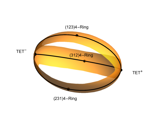
Figure 7. Part of the configuration space for $N=4$

We consider the reduced superlevel sets $\operatorname{BConf}(4)[r]$. Since $\operatorname{Conf}(4)$ is $8$-dimensional, away from the critical values these spaces are $5$-dimensional manifolds with boundary.

If we ignore the labelling of points and classify the contact graphs for four vertices, there are exactly two geometrically distinct $\rho$-critical $4$-configurations in $\operatorname{BConf}(4)$:

1. The $4$-Ring of four equally spaced points around a great circle on $\SS^{2}$ with $\theta=\frac{\pi}{2}$ which is a saddle configuration for $\rho$. There is a $1$-dimensional subspace of the tangent space to $\operatorname{BConf}(4)$ at the $4$-Ring along which $\rho$ increases to second order, i.e. the co-index is $k=1$. The critical value for $r$ for the $4$-Ring is $r_{1}=1+2\sqrt{2}\approx 3.8284$.

2. The vertices of the regular tetrahedron TET with $\theta=\cos^{-1}(-\frac{1}{3})$, which is the maximizing configuration for $\rho$ on $\operatorname{BConf}(4)$, i.e the co-index $k=0$. The critical value for $r$ for TET is $r_{2}=r_{max}(4)=2+\sqrt{6}\approx 4.4495.$

There are two intervals $(0,r_{1})$ and $(r_{1},r_{2}]$ on which the topology of $\operatorname{BConf}(4)[r]$ remains constant. From Theorem  4.3, it can be seen that on the interval $(0,r_{1})$, $\operatorname{BConf}(4)[r]$ is homeomorphic to $\operatorname{BConf}(4)$. This has the homotopy type of ${\mathbb{R}}^{2}$ punctured at two points, hence

$$H^{0}(\operatorname{BConf}(4)[r],\mathbb{Z})=\mathbb{Z},\quad H^{1}(\operatorname{BConf}(4)[r],\mathbb{Z})=\mathbb{Z}^{2},\quad H^{k}(\operatorname{BConf}(4)[r],\mathbb{Z})=0,\,\mbox{for}\,\,k\geq 2.$$

On the open interval $(r_{1},r_{2})$, the manifold $\operatorname{BConf}(4)[r]$ has two connected components, each diffeomorphic to a $5$-ball, which can be seen from the strong deformation retraction to $\operatorname{BConf}(4)[r_{2}]$ consisting of the two points associated to the orientated labelings of TET configurations, $\textrm{TET}^{+}$ and $\textrm{TET}^{-}$. Hence

$$H^{0}(\operatorname{BConf}(4)[r],\mathbb{Z})=\mathbb{Z}^{2},\quad H^{k}(\operatorname{BConf}(4)[r],\mathbb{Z})=0,\,\mbox{for}\,\,k\geq 1.$$

Figure  7 above is only a schematic picture, since we cannot draw a $5$-dimensional manifold. It compresses four of the dimensions. The visible points take $r$-values with $r_{1}\leq r\leq r_{2}$. The value $r=r_{1}$ is a circular vertical ring in the middle, and the values of $r$ increase as one moves to the left or right, reaching a maximum at $\textrm{TET}^{+}$ and at $\textrm{TET}^{-}$.

From Table  4, we can easily compute the Euler characteristic $\chi(\operatorname{BConf}(4))=-1$. The indexed sum of critical points of the function $\rho:\operatorname{BConf}(4)\rightarrow{\mathbb{R}}$ gives an alternative computation of the Euler characteristic as

$$\chi(\operatorname{BConf}(4))=\sum_{k}(-1)^{k}\#(\,\textrm{critical points of co-index = }k\,).$$

We count the labeled configurations in $\operatorname{BConf}(4)$: since the $4$-Ring has symmetry group  $D_{4}$ of order $8$ in $SO(3)$, there are $3=|\Sigma_{4}/D_{4}|$ critical points of this type with co-index $1$; and since TET has symmetry group $A_{4}$ of order $12$ in $SO(3)$, there are really $2=|\Sigma_{4}/A_{4}|$ critical points of this type with co-index $0$; and so we obtain

$$\chi(\operatorname{BConf}(4))=2-3=-1,$$

as predicted. In fact, the Morse complex for $\rho$ captures the fact that $\operatorname{BConf}(4)$ itself has the homotopy type of the $\Theta$-graph: there are $2$ vertices ($0$-cells) in the complex corresponding to the maxima (co-index $0$) $\textrm{TET}^{+}$ and $\textrm{TET}^{-}$ configurations; there are $3$ edges ($1$-cells) corresponding to the $3$ saddle (co-index $1$) $4$-Ring configurations.

4.7. Topology Change for Variable Radius: $N\geq 5$

The complexity of the changes in topology of the configuration space grows rapidly with $N$. For larger values of $N$ there are many $\rho$-critical configurations which are not maximal.

The value $N=12$ is large enough to be extremely challenging to obtain a complete analysis of the critical configurations of the configuration space, and to analyze the variation of the topology as a function of the radius $r$. The Betti numbers for $N=12$ for radius $r=0$ given in Table  4 differ greatly from those at $r=r_{max}(12)$ where the cohomology of $\operatorname{BConf}(12)[r_{max}(12)]$ is entirely in dimension $0$, according to the Purity Property, which holds for $N=12$ by results in Section  3. This topology change involves millions of (labeled) critical points. Its full investigation remains a task for the future.

5. Unit Radius Configuration Space for $12$ Spheres

In this section, we discuss $\operatorname{Conf}(12)[1]$ and $\operatorname{BConf}(12)[1]$, the configuration spaces of $12$ unit spheres touching a central unit sphere $\SS^{2}$. These configuration spaces are remarkable and have some special properties. The value $r=1$ is a critical value and that $\operatorname{BConf}(12)[1]$ has (at least) two geometrically distinct critical points, the $\operatorname{FCC}$ and $\operatorname{HCP}$ configurations. We believe that $r=1$ is the maximal radius where the spheres $\operatorname{BConf}(12)[r]$ are arbitrarily permutable with motions remaining on $\SS^{2}$ (see Section  6.5).

The case where all spheres are unit spheres has been extensively studied in connection with sphere packing. The value $r=1$ is a critical value of the radius function  $r$, and we will see that the associated configuration spaces $\operatorname{Conf}(12)[1]$ and $\operatorname{BConf}(12)[1]$ are not manifolds. To better understand their topology, it is useful to consider the spaces $\operatorname{Conf}(12)[r]$ and $\operatorname{BConf}(12)[r]$ for $r$ in a neighborhood of $1$. These are stratified spaces naturally embedded in $(\SS^{2})^{12}$ and filtered by $r$. For noncritical values of $r$, the spaces $\operatorname{Conf}(12)[r]$ and $\operatorname{BConf}(12)[r]$ are submanifolds with boundary. For all $r<r_{max}(12)$, the space $\operatorname{Conf}(12)[r]$ has top dimension $24$. After factoring out the ambient $SO(3)$-action, the space $\operatorname{BConf}(12)[r]$ has top dimension $21$.

5.1. Three Remarkable Configurations of Unit Spheres: DOD, FCP, HCC

We now consider the three configurations of $12$ touching spheres singled out by Frank (1952)  [40]. In Figure  8, the three polyhedra have vertices located at the $12$ touching sphere centers of these configurations and centroids located at the center of the central sphere. The edges of these polyhedra specify the contact graphs of these configurations, also pictured schematically in Figure  8. The $\operatorname{DOD}$ configuration realizes the optimal contact graph for $N=12$ given in Figure  5 in Section  3.3.

• The $\operatorname{DOD}$ configuration is obtained by placing $12$ spheres touching a central $13$-th sphere at the vertices of an inscribed icosahedron; such touching points are also the centers of the faces of a circumscribed dodecahedron. It has oriented symmetry group $A_{5}$, the icosahedral group, of order $60$ and in $\operatorname{BConf}(12)[1]$ there are $\frac{|\Sigma_{12}|}{|A_{5}|}=\frac{12!}{60}=7983360$ of these.

• The $\operatorname{FCC}$ configuration is obtained by stacking three layers of the hexagonal lattice, with the third layer not lying over the first layer. The inscribed polyhedron formed by the convex hull of the $12$ points of the $\operatorname{FCC}$ configuration where the spheres touch the central sphere is a cuboctahedron. The circumscribed dual polyhedron which has the $12$ points as the center of its faces is a rhombic dodecahedron. It has oriented symmetry group $\Sigma_{4}$, the octahedral group, of order $24$ and in $\operatorname{BConf}(12)[1]$ there are $\frac{|\Sigma_{12}|}{|\Sigma_{4}|}=\frac{12!}{24}=19958400$ of these.

• The $\operatorname{HCP}$ configuration is obtained by stacking three layers of the hexagonal lattice, with the third layer lying directly over the first layer. The inscribed polyhedron formed by the convex hull of the $12$ points of $\operatorname{HCP}$ where the spheres touch the central sphere is a triangular orthobicupola. This polyhedron is the Johnson solid $J_{27}$. The circumscribed dual polyhedron which has the $12$ points as the center of its faces is a trapezoidal rhombic dodecahedron. It has oriented symmetry group $D_{3}$, the dihedral group of order $6$, and in $\operatorname{BConf}(12)[1]$ there are $\frac{|\Sigma_{12}|}{|D_{3}|}=\frac{12!}{6}=79833600$ of these.

The $\operatorname{DOD}$ configuration is an interior point of $\operatorname{BConf}(12)[1]$, while the $\operatorname{FCC}$ and $\operatorname{HCP}$ configurations are elements of $\partial\operatorname{BConf}(12)[1]$.

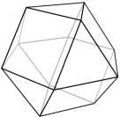
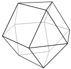
Figure 8. The DOD, FCC, and HCP configurations with their corresponding contact graphs

5.2. Three Remarkable Configurations of Unit Spheres: Rigidity Properties

We first consider rigidity properties of these packings. In the following definition we identify a sphere tangent to the $2$-sphere with the circular disk (i.e. spherical cap) on $\SS^{2}$ that it produces by radial projection.

Definition 5.1.

(cf. Connelly  [19, p. 1863]) A packing of disks on $\SS^{2}$ is locally jammed if each disk is held fixed by its neighbors. That is, no disk in the packing can be moved if all the other disks are held fixed. We say a configuration of disks is jammed if it can only be moved by rigid motions. We call it completely unjammed if each disk can be moved slightly while holding all the other disks fixed.

Theorem 5.2.

The $\operatorname{DOD}$ configuration in $\operatorname{Conf}(12)[1]$ is completely unjammed. Its space of (infinitesimal) deformations has dimension $24$. The deformation space is $21$ dimensional if viewed in $\operatorname{BConf}(12)[1]$.

Proof.

The maximal radius for $12$ spheres is $r_{\max}(12)>1$ and is achieved in the $\operatorname{DOD}$ configuration. Therefore the deformation space at $\operatorname{DOD}$ is full dimensional. ∎

In contrast, both the $\operatorname{FCC}$ and $\operatorname{HCP}$ configurations are locally jammed, i.e. they are rigid against motion of any one disk while holding all the other disks fixed; each of their infinitesimal deformation spaces has codimension at least $2$.

In Section  5.4, we will describe a deformation of the $\operatorname{DOD}$ packing to the $\operatorname{FCC}$ packing. This deformation, properly adjusted, has $6$ moving balls during its final phase arriving at $\operatorname{FCC}$. (The $6$ fixed balls form an antipodal pair of “triangles”.) We believe this value $6$ to be the smallest number of moving balls needed to unjam the $\operatorname{FCC}$ configuration. For a manual on how to unlock $\operatorname{FCC}$, see Section  8.

A deformation of the $\operatorname{DOD}$ configuration to the $\operatorname{HCP}$ configuration, also described in Section  5.4, requires $9$ moving balls at the instant of arrival at $\operatorname{HCP}$. We believe this value  $9$ to be the smallest number of moving balls needed to unjam the $\operatorname{HCP}$ configuration. For a manual on how to unlock $\operatorname{HCP}$, see Section  8. A possible reason for the larger number of moving balls needed to unjam the $\operatorname{HCP}$ configuration compared with that of the $\operatorname{FCC}$ configuration is that the $\operatorname{HCP}$ configuration has fewer local symmetries.

5.3. Three Remarkable Configurations of Unit Spheres: Criticality Properties

The $\operatorname{FCC}$ and $\operatorname{HCP}$ configurations are critical configurations for $r=1$. According to Theorem  4.11 it suffices to show that these configurations carry balanced contact graph structures.

Theorem 5.3.

The $\operatorname{FCC}$ configuration and $\operatorname{HCP}$ configuration for $r=1$ carry balanced contact graph structures. Consequently, $r=1$ is a critical value of the radius function on $\operatorname{BConf}(12)$.

Proof.

By Theorem  4.11, a sufficient condition for the criticality of a configuration for maximizing injectivity radius is that its contact graph can be balanced. That is, a set of positive weights may be assigned to the edges of the contact graph so that at each vertex the weighted vector sum, defined by the outward tangent vectors to the incident edges, vanishes.

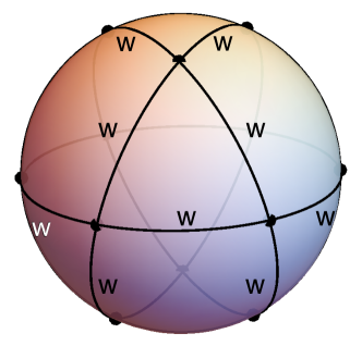
(a) FCC Configuration
     
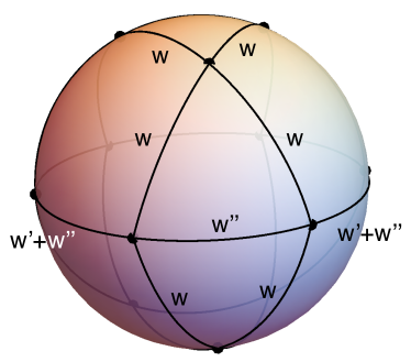
(b) HCP Configuration

Figure 9. Stress graphs for $\operatorname{FCC}$ and $\operatorname{HCP}$ configurations

We now indicate weight values for the $\operatorname{FCC}$ and $\operatorname{HCP}$ configurations (see Figure  9).

(1) At radius $r=1$ for the $\operatorname{FCC}$ configuration, the stress graph is balanced when all the weights are equal. This can be seen from the cubic- or $\Sigma_{4}$-symmetry of the contact graph.

(2) At radius $r=1$ for the $\operatorname{HCP}$ configuration, consider a weight $w_{1}$ on edges between triangular faces and square faces, a weight $w_{2}$ on edges between pairs of square faces, and a weight $w_{3}$ on edges between pairs of triangular faces. From the structure of the contact graph, it is possible to choose a constant $w_{1}>0$ and find a weight $w_{2}=w^{\prime}>0$ which balances the associated stress graph. This suffices to balance this configuration with some zero weights. However, it is also possible to add a uniform constant weight $w^{\prime\prime}=w_{3}>0$ to the equatorial great circle, giving a balanced stress graph with positive weights on all edges of $w_{1},w_{2}:=w^{\prime}+w^{\prime\prime},w_{3}:=w^{\prime\prime}$. ∎

The $\operatorname{DOD}$ configuration is not a critical configuration for $r=1$; instead it is a critical configuration at the maximal radius $r=r_{max}(12)\approx 1.10851$. As noted in Section  2, Fejes Tóth  [34] conjectured that this configuration does have a certain extremality property for local packing by equal spheres, that it gives a minimizer for a single Voronoi cell of a unit sphere packing. This statement, the Dodecahedral Conjecture, was proved in 2010 by Hales and McLaughlin  [52].

Theorem 5.4.

(Hales and McLaughlin (2010)) A $\operatorname{DOD}$ configuration of unit spheres minimizes the volume of a Voronoi cell of a unit sphere with center at the origin of ${\mathbb{R}}^{3}$ over all sphere packing configurations of unit spheres containing that sphere.

The volume of this Voronoi cell gives a local sphere packing density of approximately $0.7546$, which exceeds the sphere packing density $\frac{\pi}{\sqrt{18}}\approx 0.74048$ in $3$-dimensional space.

5.4. Three Remarkable Configurations of Unit Spheres: Deformation Properties

We now show that the $\operatorname{DOD}$ configuration can be continuously deformed inside $\operatorname{BConf}(12)[1]$ to the $\operatorname{FCC}$ configuration and to the $\operatorname{HCP}$ configuration.

Theorem 5.5.

$(1)$ On the space $\operatorname{Conf}(12)[1]$ there is a continuous deformation of the $\operatorname{DOD}$ configuration to the $\operatorname{FCC}$ configuration that remains in the interior $\operatorname{Conf}^{+}(12)[1]$ of $\operatorname{Conf}(12)[1]$ till the final instant.

$(2)$ There is also a continuous deformation of the $\operatorname{DOD}$ configuration to the $\operatorname{HCP}$ configuration that remains in the interior $\operatorname{Conf}^{+}(12)[1]$ of $\operatorname{Conf}(12)[1]$ till the final instant.

The motions of these two deformations, measured from the touching points of the $12$ spheres to the central sphere, can be given by piecewise analytic functions on the $2$-sphere. The proof of Theorem  5.5 is given in Sections  5.4.1 -  5.4.6. An unlocking manual for doing it is given in the Appendix (Section  8).

5.4.1. Coordinates for the icosahedral configuration $\operatorname{DOD}$

To describe the deformations we will need coordinates. In Sections  5.4.1 -  5.4.5 we suppose a ball with radius $1$ centered at $0$ touches all the $12$ balls of the same given radius $r$. We initially allow all values of $r\in(0,r_{max}(12)]$, but in the move $M_{6}$ described in later subsections we will necessarily restrict to $r\leq 1$. We take $\operatorname{DOD}$ to consist of $12$ equal balls of radius $r$, touching a central unit sphere at $12$ vertices of an inscribed icosahedron $I$. We view this icosahedron $I$ as embedded in $\mathbb{R}^{3}$ with Cartesian coordinates so that we have:

• Its centroid is at the center $(0,0,0)$ of the unit sphere.

• It has two opposite faces parallel to the $xy$-plane. In other words, for some $z=h$, the intersections $I\cap\mathopen{}\mathclose{{}\left\{z=\pm h}\right\}$ are triangular faces of $I.$ Here $h=\frac{\phi^{2}}{\sqrt{3\phi^{2}+3}}\approx 0.79659,$ where $\phi=\frac{1+\sqrt{5}}{2}$ is the golden ratio.

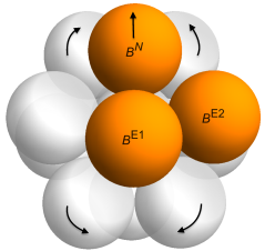
(a) Phase 1

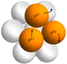
(b) Phase 2

Figure 10. The $6$-move $M_{6}$

The north balls are those which have their centers in the plane $\mathopen{}\mathclose{{}\left\{z=h}\right\},$ while the south balls have their centers in the plane $\mathopen{}\mathclose{{}\left\{z=-h}\right\}.$ The three north balls form a north triangle which is centrally symmetric to the south triangle formed by the three south balls, as in $\operatorname{FCC}$. Together with north and south triangles, we have $6$ remaining balls, which will be called equatorial, even though in the initial configuration they do not have their centers on the equator. The equator lies in the plane $z=0$.

To fix their positions, let the Greenwich meridian be defined as $\SS^{2}\cap\mathopen{}\mathclose{{}\left\{x\geq 0,\ y=0}\right\},$ and the longitude $\varphi\in[0,2\pi)$ be measured from it in the counterclockwise direction viewed from the north pole $(0,0,1)$. We require:

• The center of one of the north balls is in the half-plane of the Greenwich meridian, i.e. this ball touches the Greenwich meridian. Let us call this ball $\operatorname{B}^{N}.$

• The center of one of the equatorial balls is in the half-plane of the Greenwich meridian. Let us call it $\operatorname{B}^{E1}.$ It will necessarily be in the southern hemisphere.

This fixes the location of all $12$ balls. With this orientation of the icosahedron, the meridians of the north triangle are spaced by $\frac{2\pi}{3}.$ Furthermore the meridians of the other three balls in the northern hemisphere are also spaced by $\frac{2\pi}{3}$ and the meridians combined are spaced by  $\frac{\pi}{3}$ as in $\operatorname{FCC}$. The same holds for the six balls in the southern hemisphere.

5.4.2. The $M_{6}$-move: two variants

We now define the “$6$-move” deformation $M_{6}$, which has two variants, one leading from $\operatorname{DOD}$ to the $\operatorname{FCC}$ configuration, and the other leading to the $\operatorname{HCP}$ configuration. This move proceeds in two phases.

The first phase is the same for both variants. It moves the $6$ balls that are not equatorial at constant speed along meridians towards the poles, until they form north and south triangles of three mutually touching balls. The $6$ equatorial balls do not move.

In the second phase, all $12$ balls are moving. In both variants, the $6$ equatorial balls, initially not on the equator, move towards the equator along their meridians at constant speed, to arrive on the equator at the end of the move, forming a ring of six balls on the equator. This ring is an allowed configuration only if $r\leq 1.$ They do not touch during this move, until the last moment, and then all touch if $r=1$. At the same time, the north and south triangles will rotate about the polar axis at a variable speed, the same for all six, in such a way as to avoid the equatorial balls. They will rotate by $\frac{\pi}{3}$ to their final position. For the $\operatorname{FCC}$ move, the north triangle and south triangle rotate in the same direction, while for the $\operatorname{HCP}$ move they rotate in opposite directions. A key issue is to suitably specify the variable speed of rotation.

5.4.3. Frst phase of the $M_{6}$-move: two triangles move away from the equator

Denote by $P$ the parallel $z=z_{1}$ where the three centers of the north triangle stop. Let $-P$ be the parallel $z=-z_{1}$ where the south triangle stops.

5.4.4. Second phase of the $M_{6}$-move: rotating the two triangles

Each of the six centers of the equatorial balls, initially not on the equator, will move at constant speed along their respective meridians towards their final positions on the equator. Parametrize this motion so that at $t=0$, the $6$ balls are at their initial positions, while at $t=1$, the $6$ balls are at their final positions on the equator.

The centers of the north triangle are on $P$ at $t=0$ and will remain on $P$ throughout the move. Similarly, the centers of the south triangle are on $-P$ at $t=0$ and will remain on $-P$ throughout the move. The triangles simply rotate.

It now suffices to specify functions $\varphi^{N}\mathopen{}\mathclose{{}\left(t}\right)$, which describe the increment of the longitude of the north triangle during the time $\mathopen{}\mathclose{{}\left[0,t}\right]$ and $\varphi^{S}\mathopen{}\mathclose{{}\left(t}\right)$, the increment of the longitude of the south triangle during the time $\mathopen{}\mathclose{{}\left[0,t}\right]$. We will take $\varphi^{N}\mathopen{}\mathclose{{}\left(t}\right)$ to be a continuous, non-decreasing function, with $\varphi^{N}\mathopen{}\mathclose{{}\left(0}\right)=0,$ $\varphi^{N}\mathopen{}\mathclose{{}\left(1}\right)=\frac{\pi}{6}.$

We get two different moves to $\operatorname{FCC}$ and $\operatorname{HCP}$ depending on which direction the south triangle rotates. The motion $\varphi^{S}=\varphi^{N}$ will take us to $\operatorname{FCC}$, and choosing the opposite rotation $\varphi^{S}=-\varphi^{N}$ will take us to $\operatorname{HCP}$.

5.4.5. The choice of $\varphi^{N}$

The function $\varphi^{N},$ defined so that no ball from the two triangles hits any equatorial one, is certainly not unique.

Here is a minimal definition of $\varphi^{N},$ beginning at the second phase. Recall that our balls are open, and that:

• the center of one of the three north balls, $\operatorname{B}^{N}$, is on the half-plane of the Greenwich meridian.

• the center of one of the equatorial balls, $\operatorname{B}^{E1}$, is also on the half-plane of the Greenwich meridian.

• there is an equatorial ball with the longitude $\frac{\pi}{3};$ call it $\operatorname{B}^{E2}.$

Note that the center of $\operatorname{B}^{E1}$ is south of the plane $z=0,$ while that of $\operatorname{B}^{E2}$ is north of the plane $z=0$.

Throughout the second phase of $M_{6}$ the ball $\operatorname{B}^{E1}$ will move north while $\operatorname{B}^{E2}$ moves south. Let $\operatorname{B}^{E1}\mathopen{}\mathclose{{}\left(t}\right),$ $\operatorname{B}^{E2}\mathopen{}\mathclose{{}\left(t}\right)$ denote their positions, $t\in\mathopen{}\mathclose{{}\left[0,1}\right].$ Then for every $\varphi\in\mathopen{}\mathclose{{}\left[0,2\pi}\right)$ define $\operatorname{B}^{N}\mathopen{}\mathclose{{}\left(\varphi}\right)$ to be the ball with the center at $P$ and with the longitude $\varphi.$ For example, $\operatorname{B}^{N}\mathopen{}\mathclose{{}\left(0}\right)=\operatorname{B}^{N}.$

Now let us define the function $\varphi^{N}$ as follows:

$$\varphi^{N}\mathopen{}\mathclose{{}\left(t}\right)=\inf\mathopen{}\mathclose{{}\left\{\varphi\geq 0:\operatorname{B}^{N}\mathopen{}\mathclose{{}\left(\varphi}\right)\cap\operatorname{B}^{E1}\mathopen{}\mathclose{{}\left(t}\right)=\varnothing}\right\}.$$ (5.1)

Clearly, $\varphi^{N}\mathopen{}\mathclose{{}\left(t}\right)=0$ for all $t$ small enough. The only thing one needs to check is that

$$\operatorname{B}^{N}\mathopen{}\mathclose{{}\left(\varphi^{N}\mathopen{}\mathclose{{}\left(t}\right)}\right)\cap\operatorname{B}^{E2}\mathopen{}\mathclose{{}\left(t}\right)=\varnothing$$ (5.2)

holds for all $t\in\mathopen{}\mathclose{{}\left[0,1}\right]$.

Lemma 5.6.

An increment function $\varphi^{N}(\cdot)$ exists: $\varphi^{N}(t)$ as defined by (5.1) satisfies (5.2).

Proof.

We use Euler coordinates on the sphere. The latitude $\vartheta$ of the parallel $P$ is $\mathopen{}\mathclose{{}\left(\pi-\theta}\right),$ where $\theta$ satisfies

$$\sin\mathopen{}\mathclose{{}\left(\theta}\right)=\frac{1}{\sqrt{3}},\ \cos\mathopen{}\mathclose{{}\left(\theta}\right)=\sqrt{\frac{2}{3}},\ \tan\mathopen{}\mathclose{{}\left(\theta}\right)=\frac{1}{\sqrt{2}}.$$

By symmetry, it is enough to consider the movement of three balls:

• $\operatorname{B}^{N}$ on the parallel $P$. Its initial angle $\varphi\mathopen{}\mathclose{{}\left(t=0}\right)=0.$ The latitude $\vartheta$ of $\operatorname{B}^{N}$ is constant.

• $\operatorname{B}^{E1}$ on the Greenwich meridian $\varphi=0.$ Its initial latitude is $\vartheta\mathopen{}\mathclose{{}\left(t=0}\right)=\mathopen{}\mathclose{{}\left(\frac{2\pi}{3}-\theta}\right)<0$ and final latitude is $\vartheta\mathopen{}\mathclose{{}\left(t=1}\right)=0.$ On the interval, its latitude is given by $\vartheta\mathopen{}\mathclose{{}\left(t}\right)=\mathopen{}\mathclose{{}\left(\frac{2\pi}{3}-\theta}\right)t.$

• $\operatorname{B}^{E2}$ on the meridian $\varphi=\frac{\pi}{3}.$ Its initial latitude is $\vartheta\mathopen{}\mathclose{{}\left(t=0}\right)=-\mathopen{}\mathclose{{}\left(\frac{2\pi}{3}-\theta}\right)>0$ and final latitude is $\vartheta\mathopen{}\mathclose{{}\left(t=1}\right)=0.$ On the interval, its latitude is given by $\vartheta\mathopen{}\mathclose{{}\left(t}\right)=\mathopen{}\mathclose{{}\left(\theta-\frac{2\pi}{3}}\right)t.$

The function $\varphi^{N}\mathopen{}\mathclose{{}\left(t}\right)$ is uniquely defined by:

• $\varphi^{N}\mathopen{}\mathclose{{}\left(t}\right)\geq 0.$

• At every time $t<1$ and after initial contact, the ball $\operatorname{B}^{N}\mathopen{}\mathclose{{}\left(t}\right)$ touches the ball $\operatorname{B}^{E1}\mathopen{}\mathclose{{}\left(t}\right)$.

To complete the proof of Lemma  5.6 it remains to check that the balls $\operatorname{B}^{N}\mathopen{}\mathclose{{}\left(t}\right)$ and $\operatorname{B}^{E2}\mathopen{}\mathclose{{}\left(t}\right)$ of radius $r\leq 1$ are disjoint for $0<t<1$. This fact will follow from the next lemma. ∎

Lemma 5.7.

Let $0<t<1.$ Consider an isosceles spherical triangle $ABO,$ where $A$ has $\varphi=0,$ $\vartheta\mathopen{}\mathclose{{}\left(t}\right)=\mathopen{}\mathclose{{}\left(\frac{2\pi}{3}-\theta}\right)t,$ $B$ has $\varphi=\frac{\pi}{3},$ $\vartheta\mathopen{}\mathclose{{}\left(t}\right)=-\mathopen{}\mathclose{{}\left(\frac{2\pi}{3}-\theta}\right)t,$ and $O=O\mathopen{}\mathclose{{}\left(t}\right)$ is defined by $\vartheta\mathopen{}\mathclose{{}\left(O}\right)=\pi-\theta$ and the touching condition. Then $\mathopen{}\mathclose{{}\left|AO}\right|=\mathopen{}\mathclose{{}\left|BO}\right|>\frac{\pi}{3}.$

Proof.

Let $D$ be the middle point of the arc $AB.$ It does not depend on $t$ and is given by $\vartheta\mathopen{}\mathclose{{}\left(D}\right)=0,$ $\varphi\mathopen{}\mathclose{{}\left(D}\right)=\frac{\pi}{6}.$ Let $\varkappa\mathopen{}\mathclose{{}\left(t}\right)$ be the arc perpendicular to the arc $AB$ at $D.$ Then $O\mathopen{}\mathclose{{}\left(t}\right)$ is simply the intersection of $\varkappa\mathopen{}\mathclose{{}\left(t}\right)$ and the parallel $P.$

The triangle $O\mathopen{}\mathclose{{}\left(t}\right)DA\mathopen{}\mathclose{{}\left(t}\right)$ is a right triangle. Evidently, the legs $O\mathopen{}\mathclose{{}\left(t}\right)D$ and $A\mathopen{}\mathclose{{}\left(t}\right)D$ become shorter as $t$ increases. Hence the hypotenuse $O\mathopen{}\mathclose{{}\left(t}\right)A\mathopen{}\mathclose{{}\left(t}\right)$ becomes shorter as well. Since $O\mathopen{}\mathclose{{}\left(1}\right)A\mathopen{}\mathclose{{}\left(1}\right)=\frac{\pi}{3},$ the proof follows. ∎

5.4.6. Completion of proof of Theorem  5.5

Proof of Theorem  5.5.

Lemmas  5.6 and  5.7 complete a proof that there exists a deformation path from the $\operatorname{DOD}$ configuration to a $\operatorname{FCC}$ configuration and to a $\operatorname{HCP}$ configuration, respectively. However, the deformation path obtained does not satisfy one required condition of the theorem: remaining in the interior of the configuration space. It exits from the interior of $\operatorname{Conf}(12)[1]$ at the end of the first phase and remains on the boundary during the second phase: the three north balls are touching and the three south balls are touching.

We can modify the construction above so that no balls touch throughout the deformation until the final instant. To do this we halt the first phase just short of the three balls touching, at $z=1-\epsilon_{1}$. Then in the second phase, we allow $z$ to increase monotonically in the north triangle at some variable speed $\psi(t)$ as the rotation proceeds, in such a way as to avoid contact between the three north balls and the equatorial balls. The south triangle $z$ variable is to decrease monotonically in the reflected motion of $-z$ at the same time. Lemma  5.7 implies that if $z$ approaches $1$ rapidly enough in the motion that we can again avoid contact; this is an open condition at each point $t$, so by compactness of the motion interval we have a finite subcover to attain it. ∎

Remark.

(1) This motion process can be continued by concatenation with an inverse $M_{6}$ using $-\varphi(1-t)$, in such a way as to arrive back at a $\operatorname{DOD}$ configuration, differently labeled. This is possible because there are two exit directions (tangent vectors) from the $\operatorname{FCC}$ configuration and two exit directions from the $\operatorname{HCP}$ configuration in $\operatorname{BConf}(12)[1]$. Section  6.1 studies the group of permutations of the $12$ labels obtainable by such deformations.

(2) Starting from the $\operatorname{FCC}$ or $\operatorname{HCP}$ configuration, there is a reference frame in which the north triangle remains fixed. The inverse of the second phase of $M_{6}$ describes a move which unlocks the $\operatorname{FCC}$ configuration with $6$ moving balls and $6$ fixed balls, and which unlocks the $\operatorname{HCP}$ configuration with $9$ moving balls and $3$ fixed balls (see Section  8).

5.5. Buckminister Fuller’s “Jitterbug”

According to his recollection, on 25 April 1948 Buckminster Fuller found a “jitterbug” construction given by a jointed framework motion that, among other things, permits an $\operatorname{FCC}$ configuration, given as the vertices of a cuboctahedron, to be continuously deformed into a $\operatorname{DOD}$ configuration, given as the vertices of an icosahedron (see  [89, p. 273]).

In Buckminster Fuller’s construction, the joint distances remain constant during the motion, so that they can be rigid bars, while the radii of the associated touching spheres continuously contract during the deformation. At each instant during the motion the central sphere and the $12$ touching spheres can all have equal radii without overlapping, and this radius varies monotonically in time.

In retrospect one may see that it is possible to rescale space during the motion via homotheties varying in time such that all spheres retain the fixed radius $1$ throughout the deformation. In this case the joint lengths will change continuously in the motion. The rescaled motion no longer corresponds to a physical object with rigid bars, but it does give a continuous motion in the configuration space of $12$ equal spheres touching a 13-th central sphere that continuously deforms the $\operatorname{FCC}$ configuration to the $\operatorname{DOD}$ configuration.

The work of Buckminster Fuller on the “jitterbug” movable jointed framework is described in Schwabe  [89]. Fuller described it in his book Synergetics  [42, Sec. 460.00-463.00]. The construction is also described in Edmondson  [27, Chap. 11], with a detailed analysis in Verheyen  [97].

Remark.

The “jitterbug” motion immediately enters the interior $\operatorname{BConf}^{+}(12)[1]$ after the initial instant, in contrast to the “unlockings” described in Appendix 8, which adhere to its boundary.

6. Permutability of the $\operatorname{DOD}$ Configuration: Connectedness Conjectures

The number of connected components of the configuration space $\operatorname{Conf}(12)[r]$ is related to the ability to permute labeled spheres by deformations within $\operatorname{Conf}(12)[r]$. The possible permutability of the (labeled) spheres in the $\operatorname{DOD}$ configuration in $\operatorname{Conf}(12)[r]$ depends on the radius $r$ of the touching spheres.

6.1. Permutations of $\operatorname{DOD}$ Configurations for Radius $r=1$.

Conway and Sloane  [20, Chap. 1, Appendix, pp. 29–30] give a terse proof that for radius $1$ the labels on labeled spheres in $\operatorname{DOD}$ configurations can be arbitrarily permuted using continuous deformations inside the space $\operatorname{Conf}(12)[1]$.

Theorem 6.1.

(Permutability at radius $r=1$) For the radius parameter $r=1$, each labeled $\operatorname{DOD}$ configuration can be continuously deformed in the configuration space $\operatorname{BConf}(12)[1]$ to a $\operatorname{DOD}$ configuration at the same $12$ touching points with any permutation of the labeling.

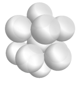
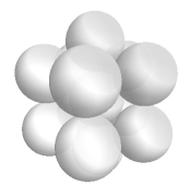
Figure 11. The $5$-move $M_{5}$

We follow the outline in Conway and Sloane  [20, Chapter 1, Appendix, pp. 29–30]. A main ingredient is an additional set of permutation moves which we call $M_{5}$-moves, detailed next.

6.2. The $M_{5}$-move

Beginning from the $\operatorname{DOD}$ configuration centered at the origin, we rotate it so that two opposite balls have their centers on the $z$ axis. Call these balls $\operatorname{N}$ and $\operatorname{S}$. Note that the centers of $5$ of the $10$ remaining balls are in the northern half-space, while the remaining $5$ centers are in the southern half-space. Call these balls $\operatorname{U}_{1}\dots\operatorname{U}_{5}$ and $\operatorname{V}_{1}\dots\operatorname{V}_{5}$, respectively.

First phase. Move the $5$ northern $\operatorname{U}_{j}$ balls towards $\operatorname{N}$, in such a way that their centers remain on their corresponding meridians, until each of them touches $\operatorname{N}$. Note that these  $5$  balls do not touch each other, only $\operatorname{N}$. Indeed, because their centers are located at the latitude $\vartheta=\frac{\pi}{6},$ when viewed from the $z$-axis each of the $5$ balls subtends the dihedral angle $\arccos\mathopen{}\mathclose{{}\left(\frac{1}{3}}\right)$ of a regular tetrahedron; but the longitude difference between the neighboring ball centers is $\frac{2\pi}{5}$, so there remains a tiny longitude gap

$$\zeta=\frac{2\pi}{5}-\arccos\mathopen{}\mathclose{{}\left(\frac{1}{3}}\right)\approx 0.025>0.$$

The $5$ southern $\operatorname{V}_{j}$ balls may be moved into the southern hemisphere in the same manner.

Second phase. Note that for $r=1$, the $6$ northern balls fit into the northern half-space, while the $6$ southern balls fit into the southern half-space. The union of all the $6$ balls in the northern hemisphere may be rotated by $\frac{2\pi}{5}$ as a rigid body, keeping the remaining balls fixed.

Third phase. Reverse the first phase.

The net result of an $M_{5}$-move is a cyclic permutation $\sigma_{2}$ of $\operatorname{DOD}$ of length $5$, which is an even permutation.

Remark.

The halfway point of a $M_{5}$ as illustrated in the right side of Figure  11 is itself a “remarkable” critical configuration; it is found at the center of a 4-simplex of critical configurations for $r=1$. The family of such configurations is in many ways similar to the maximal stratified set that occurs for $N=5$.

6.3. Proof of Permutability Theorem at Radius $r=1$

Proof of Theorem  6.1.

The first step is to show that there is a continuous deformation of $\operatorname{DOD}$ to itself, which permutes the labels by an odd permutation. To exhibit it, we use the move $M_{6},$ defined before, and deform $\operatorname{DOD}$ into an $\operatorname{FCC}$ configuration (note that we can do it for all $r\leq 1,$ but not for $r>1$). Note that the $\operatorname{FCC}$ configuration has three axes of 4-fold symmetry passing through the opposite squares of four balls. By rotating $\frac{\pi}{2}$ around any such an axis and then deforming our configuration back to $\operatorname{DOD}$ via $M_{6}^{-1},$ we induce a a permutation $\sigma_{1}$ of 12 balls, which is a product of three (disjoint) cyclic permutations, each of length 4. Every such cycle is an odd permutation, hence their product $\sigma_{1}$ is also odd.

The second step uses $M_{5}$-moves. Each such move gives a cyclic permutation of order  $5$. Since there are $12$ options for choosing $\operatorname{N}$, we get $12$ such $5$-cycles $\sigma_{2}^{\mathopen{}\mathclose{{}\left(i}\right)}$. It is shown in Conway and Sloane (using an elegant argument about the Mathieu group $M_{12}$, see  [20, pp. 328-330]) that all such $\sigma_{2}^{\mathopen{}\mathclose{{}\left(i}\right)}$ generate the alternating group $A_{12}$, the subgroup of even permutations of  $\Sigma_{12}.$

Combined with any odd permutation $\sigma_{1}$, the full permutation group $\Sigma_{12}$ is generated. ∎

6.4. Persistence of $M_{5}$-moves to some $r>1$

The move $M_{5}$ can be modified in such a way that it continues to work for all values $r\leq r_{1}$, for some $r_{1}$ slightly bigger than $1$. We first explain the modification and then propose the value of $r_{1}.$ The modification deals only with the second phase of $M_{5}$. In order to explain it, it is enough to follow the $10$ longitude values of the touching points of our balls, which may be considered as points on the equator. For $r=1$, the northern $5$ balls $\operatorname{U}_{j}$ correspond to the longitude values $u_{j},$ for $j=1,...,5,$ and we can suppose that at the initial moment these values are $u_{j}\mathopen{}\mathclose{{}\left(t=0}\right)=\mathopen{}\mathclose{{}\left(j-1}\right)\frac{2\pi}{5}.$ The longitude values $v_{j}$ are defined similarly, corresponding to the southern balls $\operatorname{V}_{j}$, and $v_{j}\mathopen{}\mathclose{{}\left(t=0}\right)=\mathopen{}\mathclose{{}\left(j-1}\right)\frac{2\pi}{5}+\frac{\pi}{5}.$ Our initial move looks now as follows:

$$u_{j}\mathopen{}\mathclose{{}\left(t}\right)=\mathopen{}\mathclose{{}\left(j-1+t}\right)\frac{2\pi}{5},\ v_{j}\mathopen{}\mathclose{{}\left(t}\right)=v_{j}\mathopen{}\mathclose{{}\left(0}\right).$$

Of course there is no need for all the $u_{j}$ to move with the same speed; the only constraint is that the difference between consecutive $u_{j}$ should equal or exceed $\arccos\mathopen{}\mathclose{{}\left(\frac{1}{3}}\right)$ at all times. In particular, we can modify the speeds in such a way that at any time $t$, we have $u_{j}\mathopen{}\mathclose{{}\left(t}\right)=v_{j}\mathopen{}\mathclose{{}\left(t}\right)$ for at most one value of $j.$

Now let the radius $r$ be slightly bigger than $1$. Then, at the moment $t$ when $u_{j}\mathopen{}\mathclose{{}\left(t}\right)=v_{j}\mathopen{}\mathclose{{}\left(t}\right),$ the corresponding balls $\operatorname{U}_{j},$ $\operatorname{V}_{j}$ will overlap.

This, however, can be remedied by making the following small deformation of our $12$-configuration:

• the ball $\operatorname{U}_{j}$ moves up along its meridian, by the distance $\mathopen{}\mathclose{{}\left(r-1}\right).$

• the ball N moves along the same meridian in the same direction by the distance $2\mathopen{}\mathclose{{}\left(r-1}\right).$

• the ball $\operatorname{V}_{j}$ moves down along its meridian, by the distance $\mathopen{}\mathclose{{}\left(r-1}\right).$

• the ball S moves along the same meridian in the same direction by the distance $2\mathopen{}\mathclose{{}\left(r-1}\right).$

• other balls may be rearranged in such a way that they do not intersect.

The non-overlap condition can be satisfied when $\mathopen{}\mathclose{{}\left(r-1}\right)>0$ is small enough, since there were no other collisions.

Below we will show there will be $5$ bottleneck configurations that one encounters on the way to perform the modified $M_{5}$ move. Each one defines a value $r_{1}^{\mathopen{}\mathclose{{}\left(j}\right)}>1$, for $1\leq j\leq 5$ which is the maximal radius for which this configuration is allowed. We set $r_{1}:=\min_{j=1,...,5}r_{1}^{\mathopen{}\mathclose{{}\left(j}\right)}>1.$

Theorem 6.2.

For every $r\leq r_{1}$ the move $M_{5}$ can be modified in such a way that one can reach from an initial labeled $\operatorname{DOD}$ configuration any labeled $\operatorname{DOD}$ configuration whose labels are an even permutation of the initial labels. That is, the alternating group $A_{12}$ is generated by the compositions of different $M_{5}$ moves.

Proof.

There will occur $5$ bottleneck $12$-configurations of the $r$-balls touching the unit central ball, described by certain touching patterns that correspond to the configurations appearing during the move $M_{5}$ at the moment when the ball $\operatorname{U}_{j}$ passes due north of the ball $\operatorname{V}_{j}.$

The $5$ bottleneck configurations have a common pattern: $4$ touching balls centered on the same meridian, two in the northern half-space, and the remaining two in the southern half-space. We denote them by $\operatorname{N}$, $\operatorname{U}_{j},$ $\operatorname{V}_{j},$ $\operatorname{S}$. This set of $4$ balls is symmetric with respect to the plane $z=0.$ Strictly speaking, as $r$ is slightly bigger than $1,$ the balls $\operatorname{N}$ and $\operatorname{S}$ are now centered on the meridian opposite the one containing $\operatorname{U}_{j}$ and $\operatorname{V}_{j}$.

The eight other balls are the remaining ones from $\operatorname{U}_{1},...\,,\operatorname{U}_{5},\operatorname{V}_{1},...\,,\operatorname{V}_{5}.$ Each pair $\{\operatorname{U}_{i}$, $\operatorname{V}_{i}\}$ touches, as do the pairs $\{\operatorname{U}_{i}$, $\operatorname{N}$}, as well as the pairs {$\operatorname{V}_{i}$, $\operatorname{S}\}$. The $5$ bottleneck configurations differ in how the additional pairs of balls touch. Each of the rows in the following list completes a different touching pattern that occurs as the move $M_{5}$ is performed:

$$\{\operatorname{U}_{1},\operatorname{U}_{2}\},\{\operatorname{V}_{2},\operatorname{U}_{3}\},\{\operatorname{V}_{3},\operatorname{U}_{4}\},\{\operatorname{V}_{4},\operatorname{U}_{5}\},\{\operatorname{V}_{5},\operatorname{V}_{1}\}, j=1$$ ()

$$\{\operatorname{U}_{2},\operatorname{U}_{3}\},\{\operatorname{V}_{3},\operatorname{U}_{4}\},\{\operatorname{V}_{4},\operatorname{U}_{5}\},\{\operatorname{V}_{5},\operatorname{V}_{1}\},\{\operatorname{U}_{1},\operatorname{U}_{2}\}, j=2$$ ()

$$\{\operatorname{U}_{3},\operatorname{U}_{4}\},\{\operatorname{V}_{4},\operatorname{U}_{5}\},\{\operatorname{V}_{5},\operatorname{V}_{1}\},\{\operatorname{U}_{1},\operatorname{V}_{2}\},\{\operatorname{U}_{2},\operatorname{U}_{3}\}, j=3$$ ()

$$\{\operatorname{U}_{4},\operatorname{U}_{5}\},\{\operatorname{V}_{5},\operatorname{V}_{1}\},\{\operatorname{U}_{1},\operatorname{V}_{2}\},\{\operatorname{U}_{2},\operatorname{V}_{3}\},\{\operatorname{U}_{3},\operatorname{U}_{4}\}, j=4$$ ()

$$\{\operatorname{V}_{5},\operatorname{V}_{1}\},\{\operatorname{U}_{1},\operatorname{V}_{2}\},\{\operatorname{U}_{2},\operatorname{V}_{3}\},\{\operatorname{U}_{3},\operatorname{V}_{4}\},\{\operatorname{U}_{4},\operatorname{U}_{5}\}. j=5$$ ()

Observe that for any $r>1$, and for any of the $5$ touching patterns, such a configuration is unique if it exists, and that it does exist for $\mathopen{}\mathclose{{}\left(r-1}\right)$ sufficiently small. We define $r_{1}^{\mathopen{}\mathclose{{}\left(j}\right)}$ as the maximal values for which the above configurations exist. ∎

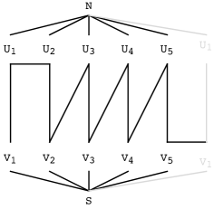
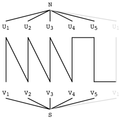
Figure 12. Contact graphs for the bottleneck configurations $j=1$ to $j=5$

We are not asserting that the value $r_{1}>1$ defined above is the true critical value above which the (small perturbation of the) move $M_{5}$ cannot be performed. Indeed, we imposed some a priori constraints in making our construction of the modified $M_{5}$, and did not rule out the possibility of a more “optimal” modification of $M_{5}$.

Definition 6.3.

Let $R_{1}$ be the maximal value of the radius $r$ for which there exists some modified move $M_{5}$. We call it the upper critical radius.

From the previous theorem we know that $R_{1}\geq r_{1}>1$. We expect $R_{1}$ to be a critical value for maximizing the radius function.

6.5. Connectedness Conjectures for $\operatorname{Conf}(12)[1]$

Based on Theorems 5.5 and  6.1 about deformation and permutability of labeled $\operatorname{DOD}$ configurations, it is natural to propose the following statement.

Conjecture 6.4.

(Connectedness Conjecture) The configuration space $\operatorname{Conf}(12)[1]$ is connected. That is, every set of $12$ distinct labeled points on the $2$-sphere pairwise separated by spherical angle at least $\frac{\pi}{3}$ can be deformed into $12$ other distinct labeled points, with all points maintaining a spherical angle at least $\frac{\pi}{3}$ apart during the deformation.

This problem appears to be approachable but difficult to prove, despite the supporting evidence of permutability in Theorem  6.1. One may approach it by cutting the space $\operatorname{BConf}(12)[r_{0}]$ into many small path-connected “convex” pieces and gluing them together in some fashion. The computational size of the problem, since the dimension of the space is  $21$, and has a complicated boundary, is daunting.

We also propose a stronger statement.

Conjecture 6.5.

(Strong Connectedness Conjecture) The radius $r=1$ is the largest radius value at which configuration space $\operatorname{Conf}(12)[r]$ is connected.

In support of Conjecture  6.5, the $M_{6}$-move appears to be possible only when $r\leq 1$. At one time instant it has $6$ spheres fitting in a ring around the equator, a condition which is allowed only for $r\leq 1$. We also know that the $r=1$ satisfies the necessary condition of being a “critical value” for the $r$-parameter.

We formulate one further conjecture concerning the connectivity structure of $\operatorname{BConf}(12)[1]$. It is based on a further analysis not included here (see  [64]), which indicates that $\operatorname{BConf}(12)[1]$ has at each of the $\frac{12!}{24}$ $\operatorname{FCC}$-configurations, and at each of the $\frac{12!}{6}$ $\operatorname{HCP}$-configurations, a unique tangent line along which it can be approached from the interior $\operatorname{BConf}^{+}(12)[1]$. In addition, this analysis shows that each of these is a local cut point, a point of a space which when removed, disconnects a small open neighborhood of the point. That is, these configurations are points at which the space $\operatorname{BConf}(12)[r]$ locally disconnects as $r$ increases past $1$. The following conjecture asserts that these local cut points form unavoidable bottlenecks in $\operatorname{BConf}(12)[1]$ in making certain rearrangements of spheres in the configuration space.

Conjecture 6.6.

($\operatorname{FCC}$ and $\operatorname{HCP}$ Bottlenecks) Any piecewise smooth continuous curve in the reduced configuration space $\operatorname{BConf}(12)[1]$ which starts at a labeled $\operatorname{DOD}$ configuration and ends at another labeled $\operatorname{DOD}$ configuration with the labels permuted by an odd permutation must necessarily pass through either an $\operatorname{FCC}$ configuration or a $\operatorname{HCP}$ configuration.

This conjecture asserts a specific way in which the $\operatorname{FCC}$ and $\operatorname{HCP}$ configurations may play a remarkable role in rearrangements of $12$-configurations, illuminating the assertion of Frank  (1952) in Section  2.7.

6.6. Disconnectedness Conjectures for $r>1$

For the region $1<r\leq R_{1}$ we propose the following conjecture.

Conjecture 6.7.

(Two Connected Components) Let $R_{1}$ be the upper critical radius defined after Theorem  6.2. Then the space $\operatorname{Conf}(12)[r]$ for $1<r<R_{1}$ has exactly two connected components. Two labeled configurations, $\operatorname{DOD}$ and $\sigma(\operatorname{DOD})$, where $\sigma\in\Sigma_{12}$ is a permutation of twelve labels, belong to different connected components of $\operatorname{Conf}(12)[r]$ if and only if the permutation $\sigma$ is odd.

In view of the existence of the $M_{5}$-move, the argument in Theorem  6.1 indicates that there can be at most $2$ connected components containing $\operatorname{DOD}$ configurations in this region. Conjecture  6.7 asserts there are exactly these two, and no other, connected components.

We next note that the five “bottlenecks” in the $5$-move lead to the possibility of connected components not containing any $\operatorname{DOD}$ configuration, for certain ranges of $r$. During the $M_{5}$ move joining two $\operatorname{DOD}$ configurations, there are $5$ bottlenecks all through which one can pass at least up to a radius $r_{1}>1$. There is however room for configurations of spheres of larger radius occurring between the bottlenecks. If we increase the radius above the smallest two of the bottleneck radii, it may be possible for a sphere to get stuck in the middle of one of these regions, so it can neither go backwards nor forwards via the $M_{5}$-move to a $\operatorname{DOD}$ configuration. Assuming that “trapped” configurations (from blocking of the $M_{5}$ move) exist containing no $\operatorname{DOD}$ configuration, eventually as we increase $r$ some “trapped” configuration must become a critical configuration. It would then be a local maximum in the configuration space, an isolated point in some $\operatorname{BConf}(12)[r]$. The critical value at which this occurs would necessarily be strictly smaller than $r_{max}(12)$, using the result of Danzer (in Theorem  3.3) that the extremal configuration for $N=12$ is unique.

Conjecture 6.8.

(Non-$\operatorname{DOD}$ Components) There is a nonempty interval of values of $r>1$ such that the reduced configuration space $\operatorname{BConf}(12)[r]$ has connected components that do not contain any copy of a $\operatorname{DOD}$ configuration.

A positive answer to this question raises the possibility of a value of $r$ for which the number of connected components of $\operatorname{BConf}(12)[r]$ exceeds the number of labeled $\operatorname{DOD}$ configurations, which is $\frac{12!}{12\times 5}=7983360$. To obtain the latter number, let us take the $\operatorname{DOD}$ configuration and label its $12$ balls. There are $12!$ such labelings. Two labeled configurations are equivalent (i.e. the same in $\operatorname{BConf}(12)[r]$) iff one can be obtained from the other by the $SO(3)$ rotation action. Clearly, there are $12\times 5$ labelings in every equivalence class.

Finally, for the region of $r$-values very close to $r_{max}(12)$, we assert that each of the spaces $\operatorname{Conf}(12)[r]$ and $\operatorname{BConf}(12)[r]$ has exactly $\frac{12!}{12\times 5}=7983360$ connected components, with each component containing a $\operatorname{DOD}$ configuration. This fact follows assuming the finiteness of the set of critical radius values $r$ for $\operatorname{BConf}(12)$, since at the point $r_{max}(12)$ only the $\operatorname{DOD}$ configurations survive, according to the uniqueness result of Danzer (Theorem  3.3), and the topology of $\operatorname{BConf}(12)[r]$ does not change above the next largest critical value of $r$ below $r_{max}(12)$.

7. Concluding Remarks

This paper treats configuration spaces of touching spheres for very small values of $N$. We have shown that the configuration space of $12$ equal spheres touching a central $13$-th sphere is already large enough to exhibit interesting behavior in its critical points. Concerning $12$-sphere configurations in the equal radius case $r=1$ we have made the following observations.

• We have clarified an assertion of Frank (1952) given in Section  2.7, showing that in the space $\operatorname{BConf}(12)[1]$ there are deformations interconnecting all $\operatorname{FCC}$, $\operatorname{HCP}$ and $\operatorname{DOD}$ configurations.

• We have given evidence suggesting that $\operatorname{BConf}(12)[1]$ is a connected space, and conjectured that $r=1$ is the largest parameter value where $\operatorname{BConf}(12)[r]$ is connected.

• We have shown that all elements of the finite set of $\operatorname{FCC}$ and $\operatorname{HCP}$ configurations lie on the boundary of the topological space $\operatorname{BConf}(12)[1]$ and are critical points for maximizing the radius parameter.

• We have conjectured that a continuous deformation of 12 spheres in a $\operatorname{DOD}$ configuration to a permutation of itself that is an odd permutation of its elements, then the deformation must pass through one of the (finite set of) $\operatorname{FCC}$ and $\operatorname{HCP}$ configurations in $\operatorname{BConf}(12)[1]$; they are “unavoidable” points.

Many challenging and computationally difficult problems remain to better understand the constrained configuration space $\operatorname{BConf}(12)[1]$.

As mentioned in the introduction, configuration spaces are of interest in physics and materials science, particularly in connection with jamming in materials. Hard sphere models which view spheres packed inside a box have been extensively studied for jamming. Materials scientists have studied configuration spaces of small numbers of hard spheres by simulation in connection with nanomaterials. Recently, Holmes-Cerfon  [57] developed an algorithm that enumerates rigid sphere clusters and has determined those with up to $16$ spheres. The cases of small numbers (but larger than the $N$ treated here) of spheres were studied in Phillips  et  al.  [82] and Glotzer et al.  [83], giving estimates for extremal configurations at values of $N$ larger than can be currently treated mathematically. We note that simulations of phase space can sample only a small part of it. In the simulation experiments reported in  [82] for $N=12$ equal spheres, the experimenters were unable to detect that the radii at which the $M_{5}$-move and the $M_{6}$-move permutation cease being feasible are in fact different (as discussed in Section  6.4).

Study of the jamming problem leads to the sub-problem concerning what is a good notion of rigidity for such configurations. There is a notion of “locally jammed configuration” in which no particle can move if its neighbors are fixed. The Tammes problem — also called the (extremal) spherical codes problem — of determining $r_{max}(N)$ is analogous to the problem of determining maximally dense jammed configurations of spheres in a box. Various notions of rigidity for spherical codes were formulated in Tarnai and Gáspár  [93]. More recently Cohn et al. [18] give a mathematical treatment of rigidity of extremal $n$-dimensional spherical codes.

In configuration theory models like $\operatorname{BConf}(N)[r]$ of this paper, critical configurations at critical values of the radius parameter might serve as a proxy for locally jammed configurations. One can view the balancing condition in Theorem  4.11 as a weak form of the locally jammed condition. However only a subclass of critical configurations will be locally jammed in the sense above.

8. Appendix: Unlocking Manual for the FCC and HCP Configurations

8.1. The $\operatorname{FCC}$ Configuration

To unlock the $\operatorname{FCC}$ configuration, a good way is to do it with the help of a friend, hereafter called Charles. Please follow these steps:

1. Ask Charles to hold the $3$ north balls and the $3$ south balls firmly in their positions. These $6$ polar balls remain fixed during the whole process. As a result, the $13$-th central ball stays fixed as well.

2. Roll the remaining $6$ equatorial balls in a direction roughly parallel to the equator. If properly lubricated, this does not require a big effort.

3. The equatorial balls can all be pushed either to the east or to the west, in a coordinated way.

4. At all times you must ensure the $6$ rolling balls touch the central ball. This requires some practice, but it is possible and not terribly hard.

5. Observe that the $6$ balls roll around the central ball along the equatorial “valley” between the polar balls kept fixed by Charles. These rolling balls cannot always move equatorially, but instead move north and south slightly, in an alternating manner, as you roll them.

6. Because the $6$ rolling balls move north and south, some of them do not touch each other any more: free space may appear between them. Also, some space can be created between them and the $6$ balls kept fixed by Charles. This is normal.

7. As you proceed by $\frac{\pi}{3},$ the $6$ rolling balls realign in the equatorial plane, touching each other and the polar balls. Note that at this moment the configuration is locked back into $\operatorname{FCC}$. Each of the $6$ rolled balls is touching two of its equatorial neighbors, one ball to the north and one ball to the south.

8.2. The $\operatorname{HCP}$ Configuration

Unlocking the $\operatorname{HCP}$ configuration is similar to the $\operatorname{FCC}$ configuration, except that Charles has somewhat more to do. Please follow these steps:

1. Ask Charles to hold firmly the three north balls and the three south balls. The three south balls will remain fixed during the whole process. But the north triangle has to be rotated as a whole in its plane, at some constant speed, which can be either eastward or westward (there are two choices). It will move through an angle $\frac{2\pi}{3}$. The $13$-th central ball stays fixed as before.

2. Roll all the remaining $6$ balls in the (roughly same) equatorial direction as the north triangle is rotating. This movement direction is forced on all six equatorial balls by the motion of the north triangle.

3. The rest of the process goes basically in the same way as for the $\operatorname{FCC}$ configuration.

4. As Charles proceeds to rotate the north triangle by $\frac{2\pi}{3}$, you proceed by $\frac{\pi}{3},$ the six middle balls align back into the equatorial plane, touching each other and the six polar balls. Note that at this moment the configuration is locked back into the $\operatorname{HCP}$ configuration. Each of the $6$ rolled balls is touching two of its equatorial neighbors, one ball to the north and one ball to the south.

Note that for $\operatorname{FCC}$, the equatorial balls underwent cyclic permutation of length $6$. For $\operatorname{HCP}$, the equatorial balls underwent a cyclic permutation of length $6$ and the $3$ northern balls a cyclic permutation of length $3$. These give odd permutations of $\operatorname{FCC}$ and $\operatorname{HCP}$.

References

[1]
A. Abrams and R. Ghrist,
Finding topology in a factory: Configuration spaces,
Amer. Math. Monthly 109 (2002), No. 2, 140–150.
[2]
H. Alpert,
Restricting cohomology classes to disk and segment
configuration spaces,
Topoogy and its Applications 230 (2017), 51–76.
[3]
P. W. Anderson,
Through the glass lightly,
Science 267 (1995), 1615.
[4]
K. Anstreicher,
The thirteen spheres: a new proof,
Disc. Comp. Geom. 31 (2004), 613–625.
[5]
C. Austin Angell,
Insights into Phases of Liquid Water from
Study of its Unusual Glass-Forming Properties,
Science 1 Feb 2008 319, 582–587.
[6]
V. I. Arnold,
The cohomology ring of dyed braids, (Russian)
Mat. Zametki 5 (1969), 227–231.
[7]
T. Aste and D. Weaire,
The Pursuit of Perfect Packing,
Institute of Physics Publishing: London 2000.
[8]
W. Barlow,
Probable nature of the internal symmetry of crystals,
Nature 29 (1883), 186–188, 205–207.
[9]
Y. Baryshnikov, P. Bubenik and M. Kahle,
Min-type Morse theory for configuration spaces of
hard spheres,
Int. Math. Res. Not. IMRN 2014 (2014), No. 9, 2577–2592.
[10]
C. Bender,
Bestimmung der grössten Anzahl gleich
grosser Kugeln, welche sich auf eine Kugel von demselben Radius,
wie die übrigen, auflegen lassen,
Acrhiv der Mathematik und Physik 56 (1874), 302–306.
[11]
K. Böröczky,
The problem of Tammes for ,
Studia Sci. Math. Hung. 18 (1983), No. 2–4, 165–171.
[12]
K. Böröczky and L. Szabó,
Arrangements of Points on a Sphere,
pp. 111-184 in A. Bezdek, Ed. Discrete Geometry,
Marcel Dekker: New York 2003.
[13]
K. Böröczky and L. Szabó,
Arrangements of and Points on a Sphere,
Studi. Sci. Math. Hung. 40 (2003), 407–421.
[14]
J. Cantarella, J. H. Fu, R. Kusner, J. M. Sullivan and N. C. Wrinkle,
Criticality for the Gehring link problem,
Geom. Topol. 10 (2006), 2055–2116.
[15]
G. Carlsson, J. Gorham, M. Kahle and J. Mason,
Computational topology for configuration spaces of hard disks,
Phys. Rev. E 85, 011303, Published 9 January 2012.
[16]
F. R. Cohen,
Artin’s braid groups, classical homotopy theory, and sundry other curiosities,
167–206 in Braids, Contemp. Math. Vol. 78:
Amer. Math. Soc. 1988.
[17]
F. R. Cohen,
Introduction to configuration spaces and their applications,
Lect. Notes Ser. Inst. Math. Sci. Natl. Univ. Singap., 19, World Sci. Publ.,
Hackensack, NJ, 2010.
[18]
H. Cohn, Yang Jian, A. Kumar and S. Torquato,
Rigidity of spherical codes,
Geometry and Topology 15 (2011), 2235–2273.
[19]
R. Connelly,
Rigidity of packings,
European Journal of Combinatorics, 29 (2008), no, 8, 1862–1871.
[20]
J. H. Conway and N. J. A. Sloane,
Sphere Packings, Lattices and Groups. Third Edition.
Springer-Verlag: New York 1998.
(First Edition: 1988).
[21]
H. S. M. Coxeter,
The problem of packing a number of equal non-overlapping circles
on a sphere, Trans. New. York Acad. Sci., Ser. II, 24 (1962), 220–231.
[22]
L. Danzer,
Endliche Punktmengen auf der -Sphäre mit möglichst grossen Minimalabstand,
Habilitationsschrift, Univ. of Göttingen, Göttingen 1963.
[23]
L. Danzer,
Finite Point-Sets on with Minimum Distance
as Large as Possible,
Discrete Math. 60(1986), 3–66.
[English translation of Danzer Habilitationsschrift, with extra references added.]
[24]
D. M. Dennison,
The crystal structure of ice,
Physical Review
17 (1921), 20-22. (Science 24 Sept. 1920 52 (1343),296–297.
[25]
A. Donev, S. Torquato, F. H. Stillinger and R. Connelly,
Jamming in hard sphere and hard disk packings,
Journal of Applied Physics 95 (2004), No. 3, 989–999.
[26]
M. D. Ediger, C. A. Angell and S. R. Nagel,
Supercooled liquids and glasses,
J. Phys. Chem. 100 (1996), 13200–13212.
[27]
A. C. Edmondson,
A Fuller Explanation: The Synergetic Geometry of R. Buckminster Fuller,
Birkhäuser: Boston 1987.
[28]
E. R. Fadell,
Homotopy groups of configuration spaces and the string problem
of Dirac,
Duke Math. J. 29 (1962), 231–242.
[29]
E. R. Fadell and S. Y. Husseini,
Geometry and Topology of configuration spaces,
Springer Monographs in Mathematics. Springer-Verlang, Berlin 2001.
[30]
E. R. Fadell and L. Newirth,