Scheduling of EV Battery Swapping, II: Distributed Solutions

Abstract

In Part I of this paper we formulate an optimal scheduling problem for battery swapping that assigns to each electric vehicle (EV) a best station to swap its depleted battery based on its current location and state of charge. The schedule aims to minimize a weighted sum of total travel distance and generation cost over both station assignments and power flow variables, subject to EV range constraints, grid operational constraints and AC power flow equations. We propose there a centralized solution based on the second-order cone programming (SOCP) relaxation of optimal power flow (OPF) and generalized Benders decomposition that is suitable when global information is available. In this paper we propose two distributed solutions based on the alternating direction method of multipliers (ADMM) and dual decomposition respectively that are suitable for cases where the distribution grid, battery stations and EVs are managed by separate entities. Our algorithms allow these entities to make individual decisions but coordinate through privacy-preserving information exchanges to jointly solve an approximate version of the joint battery swapping scheduling and OPF problem. We evaluate our algorithms through simulations.

I Introduction

I-A Motivation

In Part I of this paper we formulate an optimal scheduling problem for battery swapping that assigns to each EV a best station to swap its depleted battery based on its current location and state of charge. The station assignment not only determines EVs’ travel distance, but can also impact significantly the power flows on a distribution network because batteries are large loads. The schedule aims to minimize a weighted sum of total travel distance and generation cost over both station assignments and power flow variables, subject to EV range constraints, grid operational constraints and AC power flow equations. This joint battery swapping scheduling and OPF problem is nonconvex and computationally difficult because the AC power flow equations are nonlinear and the assignment variables are binary.

We propose in Part I a centralized solution based on the SOCP relaxation of OPF, which deals with the nonconvexity of power flow equations, and generalized Benders decomposition, which deals with the binary nature of assignment variables. When the relaxation of OPF is exact, this approach computes a global optimum. It is however suitable only for cases where the distribution network, battery stations, and EVs are managed centrally by the same operator, as is the current electric taxi program of State Grid in China. We expect that, as EVs proliferate and as battery swapping models mature, an equally (if not more) likely business model will emerge where the distribution grid is managed by a utility company, battery stations are managed by a station operator (or multiple station operators), and EVs may be managed by multiple taxi companies or by individual drivers. In particular, the set of EVs to be scheduled may include a large number of private cars in addition to fleet vehicles. The centralized approach of Part I will not be suitable for these future scenarios, for two reasons.

First, the operator in the centralized approach needs global information such as the grid topology, impedances, operational constraints, background loads, availability of fully-charged batteries at each station, locations and states of charge of EVs, etc. In the future, the grid, battery stations, and EVs will likely be operated by different entities that do not share their private information. Second, generalized Benders decomposition solves a mixed-integer convex problem in each iteration and is computationally expensive. It is hard to scale it to compute in real time an optimal station assignment and an (relaxed) OPF solution in future scenarios where the numbers of EVs and battery stations are large. In this paper we aim to develop distributed solutions that preserve private information and are more suitable for these future scenarios.

Instead of generalized Benders decomposition, we relax the binary assignment variables to real variables in $[0,1]$. With both the SOCP relaxation of OPF and the relaxation of binary variables, the resulting approximate problem of joint battery swapping scheduling and OPF is a convex program. This allows us to develop two distributed solutions where different entities make their individual decisions but are coordinated through privacy-preserving information exchanges to jointly solve the global problem. The first solution is based on ADMM and is for cases where the distributed grid is managed by a utility company and all stations and EVs are managed by a station operator. Here the utility company maintains a local estimate of some aggregate assignment information that is computed by the station operator, and they exchange the aggregate information and its estimate to attain consensus. The second solution is based on dual decomposition and is for cases where the distributed grid is managed by a utility company, all battery stations by a station operator, and all EVs are individually operated. The utility company still sends its local estimate to the station operator while the station operator does not need to send the utility company the aggregate assignment information, but only some Lagrange multipliers. The station operator also broadcasts Lagrange multipliers to all EVs and individual EVs respond by sending the station operator their choices of stations for battery swapping based on the Lagrange multiplier values and their current locations and driving ranges. In both approaches, given aggregate information and Lagrange multipliers that are exchanged, different entities only need their own local states (e.g., power flow variables) and local data (e.g., impedance values, available batteries, EV locations and driving ranges) to iteratively compute their own decisions. See Fig. 1.

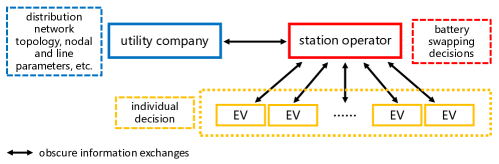
Figure 1: Distributed framework.

As we will discuss later, both distributed algorithms are able to converge to a solution, in which the station assignment may be non-binary, to the relaxed version of the joint battery swapping scheduling and OPF problem. However, we show it is easy to discretize the obtained assignment to achieve a binary one that is close to optimum, and the SOCP relaxation is usually exact [1, 2].

I-B Literature

The privacy issues in smart grids have drawn much attention from academia due to the vision of more and more interconnections in power systems to strive for strength, security, stability and efficiency [3]. Most previous work lays emphasis on the privacy issue of residential loads from the perspective of smart meters [4, 5, 6, 7], and only a small portion of the related literature realizes the significance of EVs’ privacy despite their expected high penetration in the future and the resulting giant impact on smart grids. Currently, privacy concerns for EVs mainly arise in Vehicle-to-Grid networks where the status of EVs has to be continuously monitored. Tseng [8] proposes a secure and privacy-preserving communication protocol based on restrictive partially blind signatures to protect EV owners from identity and location information leakage. Liu et al. [9] design an aggregated-proofs based authentication scheme to collect EVs’ status without revealing any individual privacy. Besides, Nicanfar et al. [10] present different situations where EVs may be involved in the smart grid context, and provide the corresponding authentication schemes to preserve EV owners’ privacy. Nonetheless, the privacy leakage of scheduling information in EV battery charging/swapping is often ignored.

In contrast to centralized algorithms, distributed (decentralized) algorithms inherently preserve privacy as global information is not necessary in local computation. Hence there is a large literature of distributed algorithm design with various applications for privacy-preserving purposes. Liu et al. [6] schedule thermostatically controlled devices and batteries in a household to hide its actual load profiles such that no privacy can be inferred from electricity usage. Yang et al. [7] design an online control algorithm of batteries that only uses the observations of the current load requirement and electricity price to strike a tradeoff between the smart meter data privacy and the electricity bill for customers. Clifton et al. [11] present a toolkit of distributed algorithms that can be combined for specific privacy-preserving data mining applications. Zhou et al. [12] devise a multi-level privacy-preserving cooperative authentication scheme to realize different levels of privacy requirement for a distributed m-healthcare cloud computing system that shares personal health information among healthcare providers. Liu et al. [13] propose a consensus-based distributed speed advisory system that optimally determines a common speed for a given area in a privacy-aware manner to minimize the group emissions of fuel vehicles or the group battery consumptions of EVs.

The remainder of this paper is organized as follows. We revisit the problem formulation in Sec. II. The proposed distributed solutions via ADMM and dual decomposition are elaborated in Sec. III, followed by numerical results in Sec. IV. At last, Sec. V concludes.

II Problem formulation

We now summarize the joint battery swapping scheduling and OPF problem in Part I [14], using the notations defined there.

An assignment of stations to EVs for battery swapping is represented by the binary variables $u:=(u_{aj},a\in\mathbb{A},j\in\mathbb{N}_{w})$ where

$$u_{aj} = \left\{\begin{split}&1\quad\mathrm{if~{}station}~{}j~{}\mathrm{is~{}assigned~{}to~{}EV}~{}a\\ &0\quad\mathrm{otherwise}\end{split}\right.$$

A station assignment must satisfy the following conditions.

• The assigned station must be in every EV’s driving range:

  $$u_{aj}d_{aj}\leq\gamma_{a}c_{a},\quad j\in\mathbb{N}_{w},a\in\mathbb{A}$$ (1a)

• Exactly one station is assigned every EV:

  $$\sum\limits_{j\in\mathbb{N}_{w}}{u_{aj}}=1,\quad a\in\mathbb{A}$$ (1b)

• Every assigned station has enough fully-charged batteries for EVs:

  $$\sum\limits_{a\in\mathbb{A}}{u_{aj}}\leq m_{j},\quad j\in\mathbb{N}_{w}$$ (1c)

A station assignment will add loads to the distribution network at buses in $\mathbb{N}_{w}$ that supply electricity to stations. The net power injections $s_{j}=p_{j}+\textbf{i}q_{j}$ depend on the station assignment $u$ according to

$$p_{j} = \left\{\begin{split}&p_{j}^{g}-p_{j}^{b}-r\left(M_{j}-m_{j}+\sum_{a\in\mathbb{A}}{u_{aj}}\right),\quad j\in\mathbb{N}_{w}\\ &p_{j}^{g}-p_{j}^{b},\quad j\in\mathbb{N}/\mathbb{N}_{w}\end{split}\right.$$ (2a)

$$q_{j} = q_{j}^{g}-q_{j}^{b},\quad j\in\mathbb{N}$$ (2b)

An active distribution network is modeled by the DistFlow equations from [15]:

$$\sum\limits_{k:(j,k)\in\mathbb{E}}{S_{jk}} =S_{ij}-z_{ij}l_{ij}+s_{j},\quad j\in\mathbb{N}$$ (3a)

$$v_{j}-v_{k} =2\mathrm{Re}(z_{jk}^{H}S_{jk})-|z_{jk}|^{2}l_{jk},\quad j\rightarrow k\in\mathbb{E}$$ (3b)

$$v_{j}l_{jk} =|S_{jk}|^{2},\quad j\rightarrow k\in\mathbb{E}$$ (3c)

The power flow quantities must satisfy the following constraints on grid operation:

• voltage stability

  $$\underline{v}_{j}\leq v_{j}\leq\overline{v}_{j},\quad j\in\mathbb{N}$$ (4a)

• generation capacity

  $$\underline{p}^{g}_{j}\leq p^{g}_{j}\leq\overline{p}^{g}_{j},\quad j\in\mathbb{N}$$ (4b)

  $$\underline{q}^{g}_{j}\leq q^{g}_{j}\leq\overline{q}^{g}_{j},\quad j\in\mathbb{N}$$ (4c)

• line transmission capacity

  $$|S_{jk}|\leq\overline{S}_{jk},\quad j\rightarrow k\in\mathbb{E}$$ (4d)

The joint battery swapping scheduling and OPF problem is to minimize a weighted sum of total generation cost in the distribution network and total travel distance of EVs over both station assignments and power flow variables:

$$\min\limits_{{u},{s},{s}^{g},\atop{v},{l},{S}} \sum\limits_{j\in\mathbb{N}}{f_{j}(p_{j}^{g})}+\alpha\sum\limits_{a\in\mathbb{A}}\sum\limits_{j\in\mathbb{N}_{w}}d_{aj}u_{aj}$$ (5)

$$\rm{s.t.} \eqref{eq:con.tax}\eqref{eq:inj}\eqref{eq:df}\eqref{eq:con.PF}$$

$$u_{aj}\in\{0,1\},\ \ a\in\mathbb{A},\,j\in\mathbb{N}_{w}$$

III Distributed solutions

III-A Relaxations

The joint battery swapping scheduling and OPF problem (5) is computationally difficult for two reasons. First, the quadratic equality (3c) is nonconvex. Second, the station assignment variables $u$ are binary.

To deal with the first difficulty, we replace (3c) by an inequality, i.e., replace the DistFlow equations (3) in the problem (5) by:

$$\sum\limits_{k:(j,k)\in\mathbb{E}}{S_{jk}} =S_{ij}-z_{ij}l_{ij}+s_{j},\quad j\in\mathbb{N}$$ (6a)

$$v_{j}-v_{k} =2\mathrm{Re}(z_{jk}^{H}S_{jk})-|z_{jk}|^{2}l_{jk},\quad j\rightarrow k\in\mathbb{E}$$ (6b)

$$v_{j}l_{jk} \geq|S_{jk}|^{2},\quad j\rightarrow k\in\mathbb{E}$$ (6c)

Fixing any assignment $u\in\{0,1\}^{AN_{w}}$, the optimization problem is then a convex problem. If an optimal solution to the SOCP relaxation attains equality in (6c) then the solution also satisfies (3) and is therefore optimal (for the given $u$). In this case, we say that the SOCP relaxation is exact. Sufficient conditions are known that guarantee the exactness of the SOCP relaxation; see [1, 2] for a comprehensive tutorial and references therein. Even when these conditions are not satisfied, SOCP relaxation for practical radial networks is still often exact, as confirmed also by our simulations in Sec. IV.

To deal with the second difficulty, we use generalized Benders decomposition in Part I [14]. This approach computes an optimal solution when SOCP relaxation is exact, but it is computationally expensive as it requires solving a binary linear program (as well as an SOCP relaxation) in each iteration of the generalized Benders decomposition procedure. Moreover, the computation is centralized and is suitable only when a single organization, e.g., State Grid in China, operates all of the distribution grid, stations, and EVs.

In this paper, we develop distributed solutions that are suitable for cases where these three are operated by different organizations that do not share their private information. To deal with the second difficulty, we relax the binary variables $u_{aj}$ to real variables $u_{aj}\in[0,1]$, $a\in\mathbb{A},~{}j\in\mathbb{N}_{w}$. The constraints (II) are then replaced by:

$$\!\!\!\!\!\!\!\!u_{aj}\in\left[0,1\right],\ u_{aj}=0\ \mathrm{if}~{}d_{aj}>\gamma_{a}c_{a}, j\in\mathbb{N}_{w},~{}a\in\mathbb{A}$$ (7a)

$$\sum_{j\in\mathbb{N}_{w}}u_{aj}=1, a\in\mathbb{A}$$ (7b)

$$\sum_{a\in\mathbb{A}}u_{aj}\leq m_{j}, j\in\mathbb{N}_{w}$$ (7c)

In summary, in this paper we solve the following convex relaxation of (5):

$$\min\limits_{{u},{s},{s}^{g},\atop{v},{l},{S}} \sum\limits_{j\in\mathbb{N}}{f_{j}(p_{j}^{g})}+\alpha\sum\limits_{a\in\mathbb{A}}\sum\limits_{j\in\mathbb{N}_{w}}d_{aj}u_{aj}$$ (8)

$$\rm{s.t.} \eqref{eq:inj}\eqref{eq:con.PF}\eqref{eq:df2}\eqref{eq:con.tax.2}$$

This problem has a convex objective and convex quadratical constraints. After an optimal solution $(x^{*},u^{*})$ of (8) is obtained, we check if $x^{*}$ attains equality in (6c). We also discretize $u_{aj}^{*}$ into $\{0,1\}$, e.g., by setting for each EV $a$ a single largest $u_{aj}$ to 1 and the rest to 0. An alternative is to randomize the station assignment using $u_{aj}^{*}$ as a probability distribution. As we will show later, the discretization can be readily implemented and achieve an assignment close to optimum.

III-B Distributed solution via ADMM

The problem (8) decomposes naturally into two subproblems, one on station assignments over $u$ and the other on OPF over $(s,{s}^{g},{v},{l},{S})$. The station assignment subproblem will be solved by a station operator that operates the network of stations. The OPF subproblem will be solved by a utility company. Our goal is to design a distributed algorithm for them to jointly solve (8) without sharing their private information.

These two subproblems are coupled only in (2a) where the utility company needs the load $r\left(M_{j}-m_{j}+\sum_{a\in\mathbb{A}}u_{aj}\right)$ of station $j$ in order to compute the net real power injection $p_{j}$. This quantity depends on the total number of EVs that each station $j$ is assigned to and is computed by the station operator. Their computation can be decoupled by introducing an auxiliary variable $w_{j}$ at each bus (station) $j$ that represents the utility company’s estimate of the quantity $r\left(M_{j}-m_{j}+\sum_{a\in\mathbb{A}}u_{aj}\right)$, and requiring that they be equal at optimality.

Specifically, recall the station assignment variables $u$, and denote the power flow variables by $x:=(w,s,{s}^{g},{v},{l},{S})$ where $w:=(r\left(M_{j}-m_{j}+\sum_{a\in\mathbb{A}}u_{aj}\right),j\in\mathbb{N}_{w})$. Separate the objective function by defining

$$f(x) := \sum\limits_{j\in\mathbb{N}}{f_{j}(p_{j}^{g})}$$

$$g(u) := \alpha\sum\limits_{a\in\mathbb{A}}\sum\limits_{j\in\mathbb{N}_{w}}d_{aj}u_{aj}$$

Replace the coupling constraints (2) by constraints local to bus $j$:

$$p_{j} = \left\{\begin{split}&p_{j}^{g}-p_{j}^{b}-w_{j},\quad j\in\mathbb{N}_{w}\\ &p_{j}^{g}-p_{j}^{b},\quad j\in\mathbb{N}/\mathbb{N}_{w}\end{split}\right.$$ (9a)

$$q_{j} = q_{j}^{g}-q_{j}^{b},\quad j\in\mathbb{N}$$ (9b)

Denote the local constraint set for $x$ by

$$\mathbb{X} := \{x\in\mathbb{R}^{(|\mathbb{N}_{w}|+5|\mathbb{N}|+3|\mathbb{E}|)}\,:\,x\text{ satisfies }\eqref{eq:con.PF}\eqref{eq:df2}\eqref{eq:tax2injw}\}$$

Denote the local constraint set for $u$ by

$$\mathbb{U} := \{u\in\mathbb{R}^{AN_{w}}\,:\,u\text{ satisfies }\eqref{eq:con.tax.2}\}$$

To simplify notation, define $u_{j}:=\sum_{a\in\mathbb{A}}u_{aj}$ for $j\in\mathbb{N}_{w}$. Then the problem (8) is equivalent to

$$\min\limits_{x,u} f(x)+g(u)$$ (10a)

$$\rm{s.t.} x\in\mathbb{X},~{}u\in\mathbb{U}$$ (10c)

$$w_{j}=r\left(M_{j}-m_{j}+u_{j}\right),\ j\in\mathbb{N}_{w}$$

We now apply ADMM to (10). Let $\lambda$ be the Lagrange multiplier vector corresponding to the coupling constraint (10c), and define the augmented Lagrangian:

$$L_{\rho}(x,{u},{\lambda}) := f(x)+g(u)+h_{\rho}(w,u,\lambda)$$ (11a)

where $$h_{\rho} (x,u) (w_{j},u_{j},j\in\mathbb{N}_{w})$$ depends on only through :

$$\begin{split}h_{\rho}(w,u,\lambda):=&\sum\limits_{j\in\mathbb{N}_{w}}\lambda_{j}[w_{j}-r\left(M_{j}-m_{j}+u_{j}\right)]\\ &+\ \frac{\rho}{2}\sum\limits_{j\in\mathbb{N}_{w}}[w_{j}-r\left(M_{j}-m_{j}+u_{j}\right)]^{2}\end{split}$$ (11b)

and $\rho$ is the step size for dual variable $\lambda$ updates. The standard ADMM procedure is to iteratively and sequentially update $(x,u,\lambda)$: for $n=0,1,\dots$,

$${x}(n+1) \!\!\!\!\!\!:=\!\!\!\!\!\! \arg\min\limits_{{x}\in\mathbb{X}}\ f(x)+h_{\rho}(w,{u}(n),{\lambda}(n))$$ (12a)

$${u}(n+1) \!\!\!\!\!\!:=\!\!\!\!\!\! \arg\min\limits_{{u}\in\mathbb{U}}\ g(u)+h_{\rho}({w}(n+1),u,{\lambda}(n))$$ (12b)

$${\lambda}_{j}(n+1) \!\!\!\!\!\!:=\!\!\!\!\!\! \lambda_{j}(n)\,+\,\rho[w_{j}(n+1)$$ (12c)

$$-r(M_{j}-m_{j}+u_{j}(n+1))],\ j\in\mathbb{N}_{w}$$

Remark 1

1. The $x$-update (12a) is carried out by the utility company and involves minimizing a convex objective with convex quadratic constraints. The $(u,\lambda)$-updates (12b)(12c) are carried out by the station operator and the $u$-update minimizes a convex quadratic objective with linear constraints. Both can be efficiently solved.

2. The $x$-update by the utility company needs $(u(n),\lambda(n))$ from the station operator in iteration $n$. In fact, from (11b), the station operator does not need to communicate the detailed station assignment $u(n)=(u_{aj}(n),\,a\in\mathbb{A},\,j\in\mathbb{N}_{w})$ to the utility company but only the total numbers of EVs $(u_{j}(n),j\in\mathbb{N}_{w})$ that stations $j$ are assigned to.

3. The $(u,\lambda)$-updates by the station operator need in iteration $n$ the utility company’s estimate $w(n+1)$ of $(r(M_{j}-m_{j}+u_{j}(n+1)),j\in\mathbb{N}_{w})$.

4. The reason that the $x$-update by the utility company needs $(u_{j}(n),j\in\mathbb{N}_{w})$ and the $u$-update by the station operator needs $w(n+1)$ is the (quadratic) regularization term in $h_{\rho}$. This becomes unnecessary for the dual decomposition approach in Sec. III-C without the regularization term.

The communication structure is illustrated in Fig. 2. In particular, private information of the utility company, such as distribution network parameters $z_{jk}$, network states $(s(n),s^{g}(n),v(n),l(n),S(n))$, cost functions $f$, and operational constraints, as well as private information of the station operator, such as the total number of batteries $(M_{j},j\in\mathbb{N}_{w})$, the numbers of available fully-charged batteries $(m_{j},j\in\mathbb{N}_{w})$, how many EVs or where they are or their states of charge, and the detailed assignment $u(n)$, do not need to be communicated.

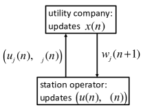
Figure 2: Communication between utility company and station operator.

When the cost functions $f_{j}$ are closed, proper and convex and $L_{0}(x,u,\lambda)$ has a saddle point, the ADMM iteration (12) converges in that, for all $j\in\mathbb{N}_{w}$, the mismatch $|w_{j}(n)-u_{j}(n)|\rightarrow 0$ and the objective $f(x(n))+g(u(n))$ converges to its minimum value [16]. This does not automatically guarantee that $(x(n),u(n))$ converges to an optimal solution to (8). If $(x(n),u(n))$ indeed converges to a primal optimal solution $(x^{*},u^{*})$, $u^{*}$ may generally not be binary. We use a heuristic to derive a binary station assignment from $u^{*}$, as mentioned above. Fortunately, the following result shows that the number of EVs $a$ for which a binary assignment needs to be derived from the obtained non-binary one $(u^{*}_{aj},j\in\mathbb{N}_{w})$ is small.

Theorem 1

Suppose $(x^{*},u^{*})$ is an optimal solution to the relaxation (8), then the number of EVs $a$ for which $u^{*}_{aj}<1$ for all $j\in\mathbb{N}_{w}$ is at most ${N_{w}(N_{w}-1)}/{2}$.

See Appendix A for its proof. In practice, the number $N_{w}$ of stations is typically small compared with the number $A$ of EVs that request battery swapping. Therefore, it is expected that the discretization will attain a station assignment close to optimum, considering the subtle impact of individual EVs.

III-C Distributed solution via dual decomposition

The ADMM-based algorithm assumes the station operator directly controls the station assignment to all EVs. This requires that the station operator know the locations ($d_{aj}$), states of charge ($c_{a}$) and performance ($\gamma_{a}$) of EVs. Moreover, the aggregate EV information $u_{j}$ needs to be provided to the utility company. We now present another algorithm based on dual decomposition that is more suitable in situations where it is undesirable or inconvenient to share private information between the utility company, the station operator, and EVs.

In the original relaxation (8), the update of the injections $p_{j}$ in (2) by the utility company involves $u_{j}$ which are updated by the station operator. These two computations are decoupled in the ADMM-based solution by introducing the auxiliary variables $w_{j}$ at the utility company and relaxing the constraint $w_{j}=r(M_{j}-m_{j}+u_{j})$. In addition, the station assignment $u$ must satisfy $u_{j}\leq m_{j}$ in (7c). This is enforced in the ADMM-based solution by the station operator that computes $u$ for the EVs. To fully distribute the computation to individual EVs, we dualize $u_{j}\leq m_{j}$ as well. Let $\lambda$ and $\mu\geq 0$ be the Lagrange multiplier vectors for the constraints $w_{j}=u_{j}$ and $u_{j}\leq m_{j}$, respectively. Intuitively $w$ and $\lambda$ decouple the computation of the utility company and that of individual EVs through coordination with the station operator. Additionally, $\mu$ decouples and coordinates the EVs’ decisions so that EVs do not need direct communication among themselves to ensure that their decisions $u_{aj}$ collectively satisfy $u_{j}\leq m_{j}$.

Consider the Lagrangian of (10) with these two sets of constraints relaxed:

$$\begin{split}L(x,{u},{\lambda},\mu):=f(x)+g(u)&+\sum\limits_{j\in\mathbb{N}_{w}}\lambda_{j}(w_{j}-r(M_{j}-m_{j}+u_{j}))\\ &+\sum\limits_{j\in\mathbb{N}_{w}}\mu_{j}(u_{j}-m_{j})\end{split}$$ (13)

and the dual problem of (10):

$$\max_{\lambda,\mu\geq 0} D(\lambda,\mu)\ :=\ \min_{x\in\mathbb{X},u\in\hat{\mathbb{U}}}\ L(x,u,\lambda,\mu)$$

where the constraint set $\hat{\mathbb{U}}$ on $u$ is:

$$\hat{\mathbb{U}} := \{u\in\mathbb{R}^{AN_{w}}\,:\,u\text{ satisfies }\eqref{eq:con.tax3.2}\eqref{eq:con.tax1.2}\}$$

Let $u_{a}:=(u_{aj},j\in\mathbb{N}_{w})$ denote the column vector of EV $a$’s decision on which station to swap its battery. Then the dual problem is separable in power flow variables $x$ as well as individual EV decisions $u_{a}$:

$$D(\lambda,\mu) =: V(\lambda)\ +\ \sum_{a\in\mathbb{A}}U_{a}(\lambda,\mu)$$ (14a)

where the problem $$V(\lambda)$$ to be solved by the utility company is:

$$V(\lambda) := \min_{x\in\mathbb{X}}\left(f(x)+\sum_{j\in\mathbb{N}_{w}}\lambda_{j}w_{j}\right)$$ (14b)

and the problem $$U_{a}(\lambda) a$$ to be solved by each individual EV is:

$$\!\!\!\!\!\!\!\!\!U_{a}(\lambda,\mu) := \min_{u_{a}\in\hat{\mathbb{U}}_{a}}\sum_{j\in\mathbb{N}_{w}}\left(\alpha d_{aj}-r\lambda_{j}+\mu_{j}\right)u_{aj}$$ (14c)

where the constraint set $$\hat{\mathbb{U}}_{a} u_{a}$$ on is:

$$\ \ \ \ \hat{\mathbb{U}}_{a}\ :=\ \Big{\{}u_{a}\in\mathbb{R}^{N_{w}}\,:\!\!\!\!\!\!\!\!\!\!\!\!\!\!\!\!\!\!\!\!\!\!\!\!\!\!\!\!\!\!\!\!\begin{split}&u_{aj}\in\left[0,1\right],\,j\in\mathbb{N}_{w}\\ &u_{aj}=0\ \mathrm{if}~{}d_{aj}>\gamma_{a}c_{a},\ j\in\mathbb{N}_{w}\\ &\sum\limits_{j\in\mathbb{N}_{w}}{u_{aj}}=1\end{split}\ \Big{\}}$$

Note that (14c) entails closed-form solutions. If there exists a unique optimal solution to $$U_{a}(\lambda,\mu) a j_{a}^{*}(\lambda,\mu)$$, i.e., for any EV there is a unique defined as

$$j_{a}^{*}(\lambda,\mu) := \arg\min_{j:d_{aj}\leq\gamma_{a}c_{a}}\{\alpha d_{aj}-r\lambda_{j}+\mu_{j}\}$$

then the optimal solution to $$U_{a}(\lambda,\mu)$$ can be uniquely determined as

$$u_{aj}(n) := \left\{\begin{array}[]{lcl}1&\text{if}&j=j_{a}^{*}(\lambda,\mu)\\ 0&\text{if}&j\neq j_{a}^{*}(\lambda,\mu)\end{array}\right.$$

i.e., it simply chooses the unique station $j_{a}^{*}$ within EV $a$’s driving range that has the minimum cost $\alpha d_{aj}-r\lambda_{j}+\mu_{j}$.

From (13) the standard dual algorithm for solving (10) is: for $j\in\mathbb{N}_{w}$,

$$\lambda_{j}(n+1):=\lambda_{j}(n)\,+\,\rho_{1}(n)[w_{j}(n)-r(M_{j}-m_{j}+u_{j}(n))]$$ (15a)

$$\mu_{j}(n+1):=\max\{\,\mu_{j}(n)\,+\,\rho_{2}(n)(u_{j}(n)-m_{j}),0\,\}$$ (15b)

where $$\rho_{1}(n),\rho_{2}(n)>0$$ are diminishing stepsizes and, from (14), we have

$$\!\!\!\!\!\!x(n) \!\!\!\!:=\!\!\!\! \arg\min_{x\in\mathbb{X}}\ \left(f(x)+\sum_{j\in\mathbb{N}_{w}}\lambda_{j}(n)w_{j}\right)$$ (15c)

$$\!\!\!\!\!\!u_{a}(n) \!\!\!\!:=\!\!\!\! \arg\min_{u_{a}\in\hat{\mathbb{U}}_{a}}\sum_{j\in\mathbb{N}_{w}}\left(\alpha d_{aj}-r\lambda_{j}+\mu_{j}\right)u_{aj},\,a\in\mathbb{A}$$ (15d)

Remark 2

1. The $x$-update (15c) is carried out by the utility company and involves minimizing a convex objective with convex quadratic constraints. The only information that is non-local to the utility company for its $x$-update is one of the dual variables $\lambda(n)$ computed by the station operator.

2. The $u_{a}$-update (15d) is carried out by each individual EV. Each EV requires the dual variables $(\lambda(n),\mu(n))$ from the station operator for its update.

3. The dual updates (15a)(15b) are carried out by the station operator which uses a (sub)gradient ascent algorithm to solve the dual problem $\max_{\lambda,\mu\geq 0}D(\lambda,\mu)$. It requires $w(n)$ from the utility company and individual decisions $u_{a}(n)$ from EVs $a$.

The communication structure is illustrated in Fig. 3.

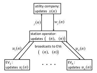
Figure 3: Communication between utility company, station operator, and EVs.

In particular, EVs are completely decoupled from the utility company and among themselves. Unlike the ADMM-based approach, the station operator knows only the (tentative) battery swapping decisions of EVs, but not their private information such as their locations ($d_{aj}$), states of charge ($c_{a}$) or performance ($\gamma_{a}$).

Since the relaxation (8) is convex, strong duality holds if Slater’s constraint qualification is satisfied. By strong duality, when the above (sub)gradient algorithm converges to a dual optimal solution $(\lambda^{*},\mu^{*})$, any primal optimal point is also a solution to the corresponding $x$-update (15c) and $u_{a}$-update (15d) [17, 18]. Suppose $(x(n),u_{a}(n),a\in\mathbb{A})$ indeed converges to a primal optimal solution $(x^{*},u_{a}^{*},a\in\mathbb{A})$, typically $(u_{a}^{*},a\in\mathbb{A})$ may not be binary. As discussed above, the discretization of $(u_{a}^{*},a\in\mathbb{A})$ can be readily implemented since Theorem 1 still holds, and in practice the gap to optimum is small.

Remark 3

The two solutions have their own advantages and can be adapted to different application scenarios. Specifically, the ADMM-based one requires a station operator that is trustworthy and can access EVs’ private information. Nonetheless, thanks to the station operator that is able to optimize the station assignment on behalf of all EVs, no computation unit is necessary on each EV’s end, and communications are only required between the station operator and the utility company, which is practical to realize. In contrast, the dual-decomposition-based one is more distributed in a sense, thus further preserving privacy inherently. However, it necessitates computation capabilities of all EVs. In addition, iterative communications, both between the station operator and the utility company and between the station operator and each individual EV, are required to enable computation. As a result, the deployment of computation units on each EV and communication unreliability may impede the practical implementation of the dual-decomposition-based solution. To conclude, the dual-decomposition-based solution further preserves privacy at the price of communication and computation overheads, compared with the ADMM-based one.

IV Numerical results

We test the two distributed algorithms on the same 56-bus radial distribution feeder of Southern California Edison (SCE) in Part I. Details about the feeder can be found in [19]. Similar setups are adopted to demonstrate the algorithm performance. 4 distributed generators and 4 stations are added to the feeder at different buses, and the 4 stations are assumed to be evenly distributed in a 4km$\times$4km square area supplied by the feeder. Table I lists their parameters. We use examples of $A=400$ EVs that request battery swapping in a certain control interval. We randomize their current locations uniformly within the square area and ignore their destinations. $d_{aj}$ is assumed to be the Euclidean distance, and the driving range constraints are readily satisfied by assuming all EVs can reach any of the 4 stations for illustrative purposes. The constant charging rate is $r=0.01$MW [20], and the weight is $\alpha=0.02$$/km [21]. Simulations are run on a laptop with Intel Core i7-3632QM CPU@2.20GHz, 8GB RAM, and 64-bit Windows 10 OS.

TABLE I: Setup

Bus	$\overline{p}_{j}^{g}$	$\underline{p}_{j}^{g}$	$\overline{q}_{j}^{g}$	$\underline{q}_{j}^{g}$	Cost function
1	4	0	2	-2	$0.3{p^{g}}^{2}+30p^{g}$
4	2.5	0	1.5	-1.5	$0.1{p^{g}}^{2}+20p^{g}$
26	2.5	0	1.5	-1.5	$0.1{p^{g}}^{2}+20p^{g}$
34	2.5	0	1.5	-1.5	$0.1{p^{g}}^{2}+20p^{g}$

(a) Distributed generator

Bus	Location	$M_{j}$	$m_{j}$
5	(1,1)	$m_{j}$	(i) $A$  ;  (ii) $A/2$
16	(3,1)	$m_{j}$	(i) $A$  ;  (ii) $A/10$
31	(1,3)	$m_{j}$	(i) $A$  ;  (ii) $A/4$
43	(3,3)	$m_{j}$	(i) $A$  ;  (ii) $A/4$

(b) Station

As shown in Table II(b), we test the two distributed algorithms using two cases (i) and (ii) of different $m_{j}$’s to show their convergence, the suboptimality they can achieve, and the exactness of SOCP relaxation.

Convergence: The convergence of the ADMM-based algorithm in case (i) is demonstrated in Fig. 4, where Fig. 4 illustrates that the Lagrange multiplier vector $\lambda$ converges rapidly and Fig. 4 shows the residual of the relaxed equality constraint (10c) diminishes acoordingly so as to attain consensus of $w$ and $(u_{j},j\in\mathbb{N}_{w})$ between the utility company and the station operator. Similar results can be found for case (ii). In terms of the dual-decomposition-based algorithm, Fig. 5 and Fig. 5 show the convergence of its two Lagrange multiplier vectors $\lambda$ and $\mu$ respectively in case (ii). $\lambda$ maintains the consensus between the utility company and EVs at convergence, and $\mu$ guarantees (7c) is satisfied when it converges. Dual decomposition usually takes more iterations to converge due to extra iterative coordination among all EVs by updating $\mu$. For case (i), results are similar except that $\mu$ remains 0 during iterations as (7c) is always satisfied.

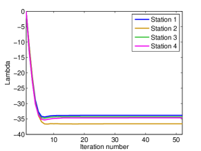
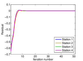
Figure 4: Convergence of ADMM (a) $\lambda$. (b) Residual.

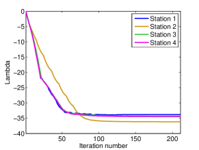
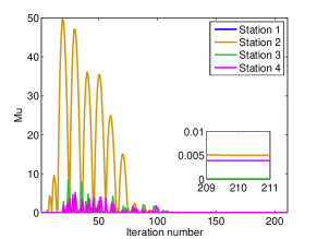
Figure 5: Convergence of dual decomposition (a) $\lambda$. (b) $\mu$.

Suboptimality (comparison with centralized solution): In case (i) both algorithms obtain a solution in which the station assignment to two EVs, marked black in Fig. 6, is non-binary, i.e., $u_{242}=[0.707~{}0.293~{}0.000~{}0.000]$ and $u_{367}=[0.230~{}0.000~{}0.770~{}0.000]$. This is consistent with Theorem 1. Unlike the centralized solution in Part I that uses global information to compute a globally optimal binary assignment, the distributed algorithms solve the relaxation (8) and are likely to attain a non-binary one, exemplified by case (i). However, we can naively round $u_{243}$ and $u_{367}$ off to discretize the assignment, as shown in Fig. 6, which turns out to be an optimal station assignment of the original problem (5), identical with the one computed by the centralized solution in Part I. Typically a heuristic binarization method will yield a suboptimal assignment, but the suboptimality gap is usually trivial due to the bounded number of EVs with a non-binary assignment and their limited impact on the whole system.

In case (ii) we reduce available fully-charged batteries at each station to activate (7c). Fig. 6 shows the solution achieved by both algorithms which contains a binary assignment, also an optimal station assignment of the original problem (5). In this case the relaxation of binary variables is exact. EVs, to which the station assignment is altered due to the bound imposed on battery availability of each station, are marked cyan in Fig. 6. The intuition is that an active (7c) sometimes can help eliminate the marginal non-binary assignment to certain EVs, and this is often the case in practice where the battery availability is uneven across stations.

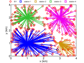
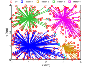
Figure 6: Suboptimality in different cases (a) case (i). (b) case (ii).

Exactness of SOCP relaxation: We check whether the above solutions computed by the distributed algorithms attain equality in (6c), i.e., whether the SOCP relaxation of OPF is exact. Our final results, as well as most tests in other case studies, confirm the exactness of the SOCP relaxation. Only partial result data for case (ii) are listed in Table II due to space limit. To sum up, the above solutions satisfy power flow equations and are thus implementable.

TABLE II: Exactness of SOCP relaxation (partial results for case (ii))

Bus		$v_{j}l_{jk}$	$|S_{jk}|^{2}$	Residual
From	To
1	2	2.582	2.582	0.000
2	3	0.006	0.006	0.000
2	4	2.336	2.336	0.000
4	5	3.413	3.413	0.000
4	6	0.005	0.005	0.000
4	7	2.276	2.276	0.000
7	8	1.984	1.984	0.000
8	9	0.009	0.009	0.000
8	10	1.518	1.518	0.000
10	11	1.318	1.318	0.000

V Concluding remarks

This paper is an extension of Part I that solves the same optimal scheduling problem for battery swapping. Instead of resorting to a centralized solution which requires global information, two distributed solutions based on ADMM and dual decomposition respectively are proposed, considering the fact that the grid, battery stations and EVs are likely operated by different entities, which do not share their private information. The distributed algorithms allow these entities to make individual decisions but coordinate through privacy-preserving information exchanges to jointly solve an approximate version of the joint battery swapping scheduling and OPF problem. Finally, the obtained station assignment may not be binary, but we prove that the number of EVs for which a binary assignment needs to be derived from the obtained non-binary one is small, and thus a station assignment that is close to optimum is expected to be attained. Numerical tests on the SCE 56-bus distribution feeder demonstrate the algorithm performance and validate our analysis.

Appendix A Proof of Theorem 1

We refer to EV $a$ as a critical EV if $u_{aj}^{*}<1$ for all $j\in\mathbb{N}_{w}$. We first show the following lemma always holds, on which basis Theorem 1 is then proved.

Lemma 1

There exists an optimal solution with no $u_{aj},u_{ak},u_{bj},u_{bk}>0$ for $\forall a,b\in\mathbb{A}$ and $\forall j,k\in\mathbb{N}_{w}$, i.e., if a solution contains two critical EVs $a,b\in\mathbb{A}$ with $u_{aj},u_{ak},u_{bj},u_{bk}>0$ for certain $j,k\in\mathbb{N}_{w}$, there always exists a better one.

Proof:

We prove Lemma 1 by contradiction.

Suppose (8) is solved by the proposed algorithms and we obtain the primal optimal solution $({u}^{*},{x}^{*})$, which contains the assignment of two stations to two same critical EVs, i.e., $u_{aj}^{*},u_{ak}^{*},u_{bj}^{*},u_{bk}^{*}>0$. We focus on the two-EV-two-station subsystem and fix its impact on the remaining parts of the whole system, e.g., the distribution network, other stations and EVs. Note that EV $a$ and EV $b$ have $rB_{a}$ and $rB_{b}$ charging loads to distribute, respectively, where $B_{a}:=u_{aj}^{*}+u_{ak}^{*}$ and $B_{b}:=u_{bj}^{*}+u_{bk}^{*}$. Meanwhile, the two EVs yield in total $rB_{j}$ and $rB_{k}$ charging loads at the buses of station $j$ and $k$, respectively, where $B_{j}:=u_{aj}^{*}+u_{bj}^{*}$ and $B_{k}:=u_{ak}^{*}+u_{bk}^{*}$. Apparently, $B_{a}+B_{b}=B_{j}+B_{k}$. Since $a$ and $b$, as well as $j$ and $k$, are indiscriminative, without loss of generality we assume case 1: $B_{a}\geq B_{j}\geq B_{k}\geq B_{b}$ and case 2: $B_{j}\geq B_{a}\geq B_{b}\geq B_{k}$ to cover all possibilities. Below we will take case 1 as an illustrative example to go on with the proof, and case 2 shares the similar property.

Obviously the above circumstance $u_{aj}^{*},u_{ak}^{*},u_{bj}^{*},u_{bk}^{*}>0$ would only occur when subcase 1’: $d_{aj}\leq d_{bj},d_{ak}\leq d_{bk}$ or subcase 2’: $d_{bj}\leq d_{aj},d_{bk}\leq d_{ak}$. Otherwise, EV $a$ and EV $b$ would have a bias for different stations in terms of the travel distance. For example, if $d_{aj}\leq d_{bj},d_{bk}\leq d_{ak}$, the two-EV-two-station subsystem will benefit if EV $a$ goes to station $j$ and EV $b$ goes to station $k$ with priority, i.e., $u^{\prime}_{aj}=B_{j},u^{\prime}_{ak}=B_{k}-B_{b},u^{\prime}_{bj}=0,u^{\prime}_{bk}=B_{b}$ with the rest of the optimal solution $({u}^{*},{x}^{*})$ is a better solution. Because the remaining parts of the whole system is not affected, which means the OPF solution and other EVs’ total travel distance won’t change, but the travel distance of the two-EV-two-station subsystem will decrease.

Again we take subcase 1’ as an example, which we call case 11’. In this case, we may have

$$\begin{split}&d_{bj}-d_{bk}>d_{aj}-d_{ak}\\ \Longleftrightarrow~{}&u_{aj}^{*}d_{aj}+u_{ak}^{*}d_{ak}+u_{bj}^{*}d_{bj}+u_{bk}^{*}d_{bk}\\ &>B_{j}d_{aj}+(B_{k}-B_{b})d_{ak}+B_{b}d_{bk}\end{split}$$ (16)

or

$$\begin{split}&d_{aj}-d_{ak}>d_{bj}-d_{bk}\\ \Longleftrightarrow~{}&u_{aj}^{*}d_{aj}+u_{ak}^{*}d_{ak}+u_{bj}^{*}d_{bj}+u_{bk}^{*}d_{bk}\\ &>(B_{j}-B_{b})d_{aj}+B_{k}d_{ak}+B_{b}d_{bj}\end{split}$$ (17)

or

$$\begin{split}&d_{aj}-d_{ak}=d_{bj}-d_{bk}\\ \Longleftrightarrow~{}&u_{aj}^{*}d_{aj}+u_{ak}^{*}d_{ak}+u_{bj}^{*}d_{bj}+u_{bk}^{*}d_{bk}\\ &=B_{j}d_{aj}+(B_{k}-B_{b})d_{ak}+B_{b}d_{bk}\\ &=(B_{j}-B_{b})d_{aj}+B_{k}d_{ak}+B_{b}d_{bj}\end{split}$$ (18)

In the cases of (16) and (17), there is a better solution that decreases the travel distance of the two-EV-two-station subsystem, while the remaining parts of the whole system remain the same. This conflicts the original assumption that $({u}^{*},{x}^{*})$ is the optimal solution. In the case of (18), still we can find solutions of equal optimum that only render either EV $a$ or EV $b$ critical.

Likewise, case 12’, case 21’ and case 22’ share the same conclusion. As a result, there always exists an optimal solution with no $u_{aj},u_{ak},u_{bj},u_{bk}>0$ for $\forall a,b\in\mathbb{A}$ and $\forall j,k\in\mathbb{N}_{w}$.

This completes the proof. ∎

Based on Lemma 1, we now go on to prove Theorem 1.

Proof:

According to the definition of a critical EV, its charging load will split into at least two parts that are distributed to different stations. The problem is currently transformed to how many critical EVs we can assign the $N_{w}$ stations to at most without violating Lemma 1.

This is a basic assignment problem. Obviously, assume every critical EV only splits into two parts at best, i.e., at most two station can be assigned to each critical EV. Then we need to assign the $N_{w}$ stations to as many critical EVs as possible without repeats. We start from assigning two consecutively indexed stations to each critical EV, i.e., stations 1 and 2 to one critical EV, and stations 2 and 3 to another, etc. Note that stations $N_{w}$ and 1 are not consecutive. By this means, we can assign stations to at most $N_{w}-1$ critical EVs. Then two stations with a one-index gap are assigned to each critical EV, i.e., stations 1 and 3 to one critical EV, and stations 2 and 4 to another, etc, by which means we can assign stations to at most $N_{w}-2$ critical EVs. By analogy, we finally assign two stations with an $(N_{w}-2)$-index gap to each critical EV, and will find there is at most only 1 critical EV that we can assign stations to. Therefore, in total we are able to assign the $N_{w}$ stations to at most $(N_{w}-1)+(N_{w}-2)+\dots+1=\frac{N_{w}(N_{w}-1)}{2}$ critical EVs, so as to satisfy Lemma 1.

This completes the proof. ∎

References

- [1] S. H. Low, “Convex relaxation of optimal power flow, I: formulations and relaxations,” IEEE Trans. on Control of Network Systems, vol. 1, no. 1, pp. 15–27, 2014.
- [2] S. H. Low, “Convex relaxation of optimal power flow, II: exactness,” IEEE Trans. on Control of Network Systems, vol. 1, no. 2, pp. 177–189, 2014.
- [3] P. McDaniel and S. McLaughlin, “Security and privacy challenges in the smart grid,” IEEE Security and Privacy, vol. 7, no. 3, pp. 75–77, 2009.
- [4] G. Kalogridis, C. Efthymiou, S. Z. Denic, T. A. Lewis, and R. Cepeda, “Privacy for smart meters: Towards undetectable appliance load signatures,” in Proc. of IEEE International Conference on Smart Grid Communications (SmartGridComm), pp. 232–237, 2010.
- [5] C. Efthymiou and G. Kalogridis, “Smart grid privacy via anonymization of smart metering data,” in Proc. of IEEE International Conference on Smart Grid Communications (SmartGridComm), pp. 238–243, 2010.
- [6] E. Liu, P. You, and P. Cheng, “Optimal privacy-preserving load scheduling in smart grid,” in Proc. of IEEE Power & Energy Society General Meeting, pp. 1–5, 2016.
- [7] L. Yang, X. Chen, J. Zhang, and H. V. Poor, “Optimal privacy-preserving energy management for smart meters,” in Proc. of IEEE Conference on Computer Communications (INFOCOM), pp. 513–521, 2014.
- [8] H.-R. Tseng, “A secure and privacy-preserving communication protocol for V2G networks,” in Proc. of IEEE Wireless Communications and Networking Conference (WCNC), pp. 2706–2711, 2012.
- [9] H. Liu, H. Ning, Y. Zhang, and L. T. Yang, “Aggregated-proofs based privacy-preserving authentication for V2G networks in the smart grid,” IEEE Trans. on Smart Grid, vol. 3, no. 4, pp. 1722–1733, 2012.
- [10] H. Nicanfar, P. TalebiFard, S. Hosseininezhad, V. Leung, and M. Damm, “Security and privacy of electric vehicles in the smart grid context: problem and solution,” in Proc. of ACM International Symposium on Design and Analysis of Intelligent Vehicular Networks and Applications, pp. 45–54, 2013.
- [11] C. Clifton, M. Kantarcioglu, J. Vaidya, X. Lin, and M. Y. Zhu, “Tools for privacy preserving distributed data mining,” ACM Sigkdd Explorations Newsletter, vol. 4, no. 2, pp. 28–34, 2002.
- [12] J. Zhou, X. Lin, X. Dong, and Z. Cao, “Psmpa: Patient self-controllable and multi-level privacy-preserving cooperative authentication in distributedm-healthcare cloud computing system,” IEEE Trans. on Parallel and Distributed Systems, vol. 26, no. 6, pp. 1693–1703, 2015.
- [13] M. Liu, R. H. Ordóñez-Hurtado, F. Wirth, Y. Gu, E. Crisostomi, and R. Shorten, “A distributed and privacy-aware speed advisory system for optimizing conventional and electric vehicle networks,” IEEE Trans. on Intelligent Transportation Systems, vol. 17, no. 5, pp. 1308–1318, 2016.
- [14] P. You, S. H. Low, W. Tushar, G. Geng, C. Yuen, Z. Yang, and Y. Sun, “Scheduling of EV battery swapping, I: centralized solution,” arXiv preprint arXiv:1611.07943, 2016.
- [15] M. E. Baran and F. F. Wu, “Optimal sizing of capacitors placed on a radial distribution system,” IEEE Trans. on Power Delivery, vol. 4, no. 1, pp. 735–743, 1989.
- [16] S. Boyd, N. Parikh, E. Chu, B. Peleato, and J. Eckstein, “Distributed optimization and statistical learning via the alternating direction method of multipliers,” Foundations and Trends® in Machine Learning, vol. 3, no. 1, pp. 1–122, 2011.
- [17] S. Boyd, L. Xiao, and A. Mutapcic, “Subgradient methods,” lecture notes of EE392o, Stanford University, Autumn Quarter, vol. 2004, pp. 2004–2005, 2003.
- [18] S. Boyd and L. Vandenberghe, Convex optimization. Cambridge university press, 2004.
- [19] M. Farivar, R. Neal, C. Clarke, and S. Low, “Optimal inverter VAR control in distribution systems with high PV penetration,” in Proc. of IEEE Power & Energy Society General Meeting, pp. 1–7, 2012.
- [20] M. Yilmaz and P. T. Krein, “Review of battery charger topologies, charging power levels, and infrastructure for plug-in electric and hybrid vehicles,” IEEE Trans. on Power Electronics, vol. 28, no. 5, pp. 2151–2169, 2013.
- [21] U. EIA, “Annual energy review,” Energy Information Administration, US Department of Energy: Washington, DC www. eia. doe. gov/emeu/aer, 2011.