Tritium $\beta$-decay in pionless effective field theory

Abstract

We calculate the $\beta$-decay of tritium at next-to-leading order in pionless effective field theory. At this order, a low-energy parameter $l_{1,A}$ enters the calculation that is also relevant for a high-accuracy prediction of the solar proton-proton fusion rate. We use the tritium half-life to determine this parameter and provide uncertainty estimates. We show proper renormalization of our calculation analyzing the residual cutoff dependence of observables. We find that next-to-leading order corrections contribute about $4\%$ to the triton decay Gamow-Teller strength. We show that these conclusions are insensitive to different arrangements of the effective range expansion.

I Introduction

Weak decays of nuclei are an everyday window to quantum-chromodynamics (QCD). This is the main reason for their extensive use in experiments that try to study the limits of the Standard Model, from measuring the masses of neutrinos using triton $\beta$-decay, to pin-pointing the basic symmetries of the theory through the dynamics of ⁶He decay. The triton $\beta$-decay, as the only $A=3$ $\beta$-decay, can, therefore, probe unique properties of the nuclear force for both ³H and ³He. Alas, since this reaction is characterized by its low-energy, i.e., $Q<10$ MeV, one cannot use QCD due to its non-perturbative character at low energies.

In the past two decades, a novel theoretical method named effective field theory (EFT) revolutionized nuclear physics. EFT is a simple, order by order, renormalizable and model-independent theoretical method that is used to describe low-energy processes. The prerequisite for describing a physical process using EFT is that its transfer momentum, $Q$, is small compared to a large scale, $\Lambda_{\rm cut}$ (i.e., $Q/\Lambda_{\rm cut}\ll 1$) Bedaque and van Kolck (2002); Kaplan et al. (1996, 1998a, 1998b, 1999) inherent to the system under consideration. This method becomes particularly useful when there is a significant scale separation between $Q$ and $\Lambda_{\rm cut}$, so that only a small number of the effective operators corresponding to the leading powers in $\frac{Q}{\Lambda_{\rm cut}}$ need to be retained to reproduce long wavelength observables with the desired accuracy.

The relevant momentum scale $Q$ is small, i.e. $Q\ll\Lambda_{\rm cut}=m_{\pi}$ tritium $\beta$-decay and for many other few-body electroweak processes of interest. In these cases, pionless EFT ($\pi\text{/}$EFT ) is an appropriate framework GriessHammer (2005); Platter (2009).

The Coulomb interaction in light nuclei is also an issue that needs to be addressed. Naïvely, the Coulomb interaction is non-perturbative at low momenta ($\lesssim 10\,\,\text{MeV}$) but should be perturbative in nuclei where the typical momenta are much higher. However, recent calculations done by König et al. König and Hammer (2011); König et al. (2015, 2016) have shown that for $A=3$, the Coulomb interaction can be treated perturbatively, as reflected in the ³H-³He binding energy difference. Moreover, in Ref. De-Leon et al. (2019), we have shown that, even though the Coulomb interaction does not conserve the three-nucleon isospin, the Coulomb energy difference can be presented in terms of a general matrix element between two $A=3$ bound-states. At LO, ³He (the lightest and, therefore, the simplest nucleus that includes a Coulomb interaction) is described correctly within $\pi\text{/}$EFT , even when the Coulomb interaction is non-perturbative Ando and Birse (2010); Gautam and Kong (2003). At next-to-leading order (NLO), the results are not so clear, and some approaches point towards the need for additional, isospin-dependent three-body forces. Therefore, other three-nucleon observables are needed to obtain predictive power within $\pi\text{/}$EFT at NLO, such as the ³He binding energy König and Hammer (2011); Vanasse et al. (2014); König et al. (2015).

One way to test the predictive power of $\pi\text{/}$EFT for the three-nucleon system at NLO, and in particular, the effect of the Coulomb interaction of such a system is through the aforementioned electroweak properties of light nuclear systems. This is the goal of this paper, in which we aim at describing tritium $\beta$-decay. This observable is particularly interesting since it is well-known experimentally, and can be used to determine the short-range strength of the axial coupling to nuclei. Specifically, the $\pi\text{/}$EFT axial-vector current contains an additional two-body operator at NLO whose low-energy constant (LEC), known as $l_{1,A}$ needs to be determined. This is in particular important for a high-accuracy description of the astrophysically relevant proton-proton fusion rate Adelberger et al. (2011); Schiavilla et al. (1998); Gazit et al. (2009); Park et al. (2003). However, its exact value is a matter of discussion in the literature Kong and Ravndal (1999a, 2001); Butler and Chen (2000, 2001); Chen et al. (2005); Ando et al. (2008) and the lack of a $\pi\text{/}$EFT calculation that is able to consistently determine this counterterm is the reason for this discussion.

Besides determining $l_{1,A}$, we will also use our work to study the convergence pattern of $\pi\text{/}$EFT for this process and analyze the residual cutoff dependence for this observable. Will also discuss the impact of the Coulomb interaction on the relevant matrix element.

This paper is organized as follows: The general formalism of $\pi\text{/}$EFT is presented in Section II. The $\pi\text{/}$EFT formalism for the weak interaction is given in Section III. The general calculation of weak matrix elements is presented in Section IV while the numerical results are given in V. In Section VI, we use the experimental value of the triton $\beta$-decay rate to fix $l_{1,A}$ at NLO. In Section. VII, we compare this approach of matching this counterterm to previous studies. We then summarize and provide an outlook in Section VIII.

II $\pi\text{/}$EFT up to next-to-leading order

Originally, $\pi\text{/}$EFT was developed in terms of nucleon fields alone. However, dynamical dibaryon fields provide a convenient way to reformulate $\pi\text{/}$EFT in a way that simplifies three-body calculations. The fields $t$ and $s$ have quantum numbers of two nucleons coupled to an S-wave spin-triplet and -singlet state, respectively. The effective masses and interaction strengths of these dibaryons are related to the two-nucleon scattering lengths and effective ranges in these two channels. This formulation is formally equivalent to the usual single-nucleon theory but in a three-nucleon calculation it reduces the problem to an effective two-body calculation.

For the construction of the $\pi\text{/}$EFT Lagrangian, we note that the external momenta $q$ and the deuteron binding momentum $\gamma_{t}$ are formally $\mathcal{O}(Q)$ ($Q$ is the typical momentum scale in the reaction), the two-nucleon scattering lengths are $\mathcal{O}(1/Q)$, and the two-nucleon effective range is $\mathcal{O}({1/\Lambda_{\rm cut}})$. Up to NLO, i.e., $\mathcal{O}(Q/\Lambda_{\rm cut})$, the two-body Lagrangian has the form Beane and Savage (2001):

$$\mathcal{L}=N^{\dagger}\left(iD_{0}+\frac{{\bf D}^{2}}{2M}\right)N-t^{i\dagger}\left[\left(iD_{0}+\frac{{\bf D}^{2}}{4M}\right)-\sigma_{t}\right]t^{i}\\ -s^{A\dagger}\left[\left(iD_{0}+\frac{{\bf D}^{2}}{4M}\right)-\sigma_{s}\right]s^{A}\\ -y_{t}\left[t^{i\dagger}\left(N^{T}P_{t}^{i}N\right)+{\rm h.c.}\right]-y_{s}\left[s^{A\dagger}\left(N^{T}P_{s}^{A}N\right)+{\rm h.c.}\right]~{},$$ (1)

where $A$ denotes the isospin triplet index, $i$ the spin-triplet index, and $N$ is the single nucleon field, of mass $M$ and $P_{t}^{i},\,P_{s}^{A}$ are the projection operators to the triplet and singlet states, respectively. We note that the minus sign in front of the kinetic terms of $s$ and $t$ implies that these fields are ghost fields. The covariant derivative is:

$$D_{\mu}=\partial_{\mu}+ieA_{\mu}\hat{Q}~{},$$ (2)

where $e$ is the electric charge and $\hat{Q}$ is the charge operator, coupled to the electromagnetic field, $A_{\mu}$.

After renormalization one finds $\sigma_{s}=\frac{2}{M\rho_{{s}}}\left(\frac{1}{a_{{s}}}-\mu\right)$, $\sigma_{t}=\frac{2}{M\rho_{{t}}}\left(\gamma_{t}-\mu\right)$, and $y_{t,s}$ are the coupling constants between two nucleons and dibaryon, $y_{t,s}=\frac{\sqrt{8\pi}}{M\sqrt{\rho_{{t,s}}}}$. The expressions above contain the singlet scattering length $a_{s}$, the deuteron binding momentum $\gamma_{t}$, and the triplet and singlet effective ranges $\rho_{t}$ and $\rho_{s}$, respectively. The deuteron binding momentum is related to the deuteron binding energy $B_{2}$ through $B_{2}=\gamma^{2}/m$. The renormalization scale $\mu$ enters these equations through the use of the power divergence subtraction scheme Kaplan et al. (1998b). To include the Coulomb interaction, we will also require the proton-proton ($pp$) scattering length $a_{C}$ and effective range $\rho_{C}$. The experimental values for the two-nucleon observables needed here are given in Tab. 1.

In this work, contrary to previous works on the electroweak properties of light nuclei, that set the renormalization group (RG) scale $\mu$ to $\mu=m_{\pi}$, we test correct renormalization by taking the UV cutoff $\Lambda$ to infinity at the end of the calculation.

Naïvely, the effective ranges are fixed from scattering experiments. However, since the triplet channel is bound, the deuteron (spin-triplet, $t$) effective range can be alternatively fixed by the long-range properties of the deuteron wave function.

The long-range properties of the deuteron wave function are set by a quantity that we will call $Z_{d}$, where $Z_{d}$ is defined through the deuteron asymptotic S-State normalization, ${A}_{S}$, such that ${A}_{S}\equiv\sqrt{2\gamma_{t}Z_{d}}$ and $Z_{d}=\frac{1}{1-\gamma_{t}\rho_{t}}\approx 1.690(3)$ Phillips et al. (2000) ($\gamma_{t}$ is the deuteron binding momentum, $\gamma_{t}=\sqrt{ME_{b}(d)}$). In the effective range expansion (ERE), the order-by-order expansion of $Z_{d}$ is:

$$\begin{split}Z_{d}^{\text{LO}}&=1~{},\\ Z_{d}^{\text{NLO}}&=1+\gamma_{t}\rho_{t}\approx 1.408\\ \end{split}$$ (3)

Parameter	Value	Reference
$\gamma_{t}$	45.701 MeV	Van Der Leun and Alderliesten (1982)
$\rho_{t}$	1.765 fm	de Swart et al. (1995)
$a_{s}$	-23.714 fm	Preston and Bhaduri
$\rho_{s}$	2.73 fm	de Swart et al. (1995)
$a_{p}$	-7.8063$\pm$0.0026 fm	Bergervoet et al. (1988)
$\rho_{C}$	2.794$\pm$0.014 fm	Bergervoet et al. (1988)

Table 1: Parameters used in the numerical calculation

This result for the perturbative expansion of the Z-factor is based on a matching of the parameters in the EFT to the effective range expansion (ERE). At NLO, the parameters can also be chosen to fix the pole position and wave function renormalization constant of the triplet two-body propagator to the deuteron values. This parameterization is known as the Z-parameterization and is advantageous because it reproduces the correct residue about the deuteron pole at NLO, instead of being approached perturbatively order by-order as in ERE-parameterization GriessHammer (2004); Kong and Ravndal (2001); Vanasse (2013); J. (2017); Phillips et al. (2000):

$$\begin{split}Z_{d}^{\text{LO}}&=1~{},\\ Z_{d}^{\text{NLO}}&=1+\left(Z_{d}^{\text{full}}-1\right)=1.690(3).\end{split}$$ (4)

The price is that the value of the triplet effective range at NLO in this parameterization is $\rho^{\prime}_{t}=\frac{Z_{d}-1}{\gamma_{t}}\approx\frac{0.690}{\gamma_{t}}=2.979\,\text{fm}$. In the following, we use both parameterizations at NLO.

II.1 $A=3$ nuclear amplitudes, matrix elements, and regularization

While an analytical result for the deuteron wave function can be derived in pionless EFT Kong and Ravndal (1999a), the three-nucleon scattering amplitude has to be calculated numerically. The different channels for ³H are the spin-triplet - $t$ (representing an “off-shell” deuteron, $d$, dibaryon), and the spin-singlet - $s$ ($nn,np$). For ³He, the contributing channels are the spin-triplet - $t$, spin-singlet - $s$ ($np$) and $pp$ Faddeev and Merkuriev (1993). The latter is required because of the Coulomb force between the protons, which modifies the long-range scattering properties of these nucleons.

The Faddeev integral equation, used in this EFT, has to be regularized. A simple way to do this is to evaluate the momentum space integrals in the integral equation up to a cutoff $\Lambda$. Since $\pi\text{/}$EFT is supposed to be order-by-order renormalizable; the theory should not depend on this ultraviolet (UV) cutoff. However, for three-nucleon systems, the numerical and theoretical solution of the integral equations displays a strong dependence on the cutoff. To overcome this problem, one adds a three-body counterterm Bedaque et al. (1999, 2000). In the case of ³He, the addition of Coulomb interaction to the three-nucleon amplitude leads to divergence in the Coulomb Feynman diagrams, which is solved by the redefinition of the proton-proton scattering length Kong and Ravndal (2000, 1999b). With this redefinition, the ³He binding energy is renormalization-group invariant at LO. König et al. (2015, 2016).

The calculation of bound-state amplitudes requires the solution of a homogeneous Faddeev equation defined up to a normalization. The calculation of next-to-leading order corrections follows the same formalism, however with a single NLO insertion, e.g., of an effective range. The three-body wave function normalizations, $Z_{{}^{3}\text{H}},\,Z_{{}^{3}\text{He}}$, are calculated diagrammatically, by summing over all possible connections between two identical vertex functions as presented in Ref. De-Leon et al. (2019).

The Coulomb force is included by considering the full $pp$ Coulomb propagator and allowing a single photon insertion in the three-body diagrams. At LO, it was shown that ³He is described correctly within $\pi\text{/}$EFT  Gautam and Kong (2003); Ando and Birse (2010); Kirscher and Gazit (2016), while at NLO, within the power counting considered here, there is a need for an additional, isospin dependent, three-body force to renormalize the ³He binding energy  König and Hammer (2011); Vanasse et al. (2014); König et al. (2015); De-Leon et al. (2019).

The nuclear amplitudes we use here are taken explicitly from Ref. De-Leon et al. (2019), where they were benchmarked numerically, and validated using the binding energy difference between ³H-³He.

III The weak interaction in $\pi\text{/}$EFT 

For low-energy charge lowering processes, the weak-interaction Hamiltonian is

$$\mathcal{H}_{\text{Weak}}=\frac{G_{F}V_{ud}}{\sqrt{2}}l_{+}^{\mu}J_{\mu}^{-},$$ (5)

where $G_{F}$ is the Fermi constant and $V_{ud}$ is the CKM matrix element. $l^{\mu}$ is the lepton current and $J_{\mu}$ is the hadronic current. We use the two-body hadronic current $J_{\mu}$ from the $\pi\text{/}$EFT effective Lagrangian with dibaryon fields up to NLO.

The hadronic current contains two parts, a polar-vector and axial-vector, $J_{\mu}=V_{\mu}-A_{\mu}$. The part of the polar vector current relevant to $\beta$-decay with a vanishing energy transfer is:

$$V_{0}^{\pm}=N^{\dagger}\frac{{\tau^{\pm}}}{2}N~{},$$ (6)

where $\tau^{\pm}=\tau_{1}\pm i\tau_{2}$.

Here, we utilized the fact that the Conserved Vector Current (CVC) hypothesis is accurate at this order of EFT.

The axial-vector part is (see Ref. Ando et al. (2008); Beane and Savage (2001)):

$$A^{\pm}_{i}=\underbrace{\frac{g_{A}}{2}N^{\dagger}\sigma_{i}\tau^{\pm}N}_{\text{LO}}+\underbrace{g_{A}L_{1,A}\left(t_{i}^{\dagger}s_{\pm}+{\rm h.c.}\right)}_{\text{NLO}}~{},$$ (7)

where $\tau^{\pm}=\tau_{1}\pm i\tau_{2}$ and $s_{\pm}=s_{1}\pm is_{2}$ and $g_{A}$ is the axial coupling constant for a single nucleon, known from neutron $\beta$-decay. We denote the coefficient of the two-body operator with $L_{1,A}$ (see Ref. De-Leon et al. (2019) for more details). A number of previous pionless EFT electroweak calculations were calculated using a Lagrangian with single nucleon fields only. The axial-vector two-body counterterm takes then the form

$$L^{\prime}_{1,A}(N^{T}P_{i}N)^{\dagger}(N^{T}P_{-}N)~{}.$$ (8)

The coefficients of these two-body operators are related through the relation

$${L_{1,A}}(\mu)=-\frac{\rho_{t}+\rho_{s}}{2\sqrt{\rho_{s}\rho_{t}}}+\frac{L^{\prime}_{1,A}}{2\pi g_{A}}\frac{1}{\sqrt{\rho_{s}\rho_{t}}}\left(\mu-\gamma_{t}\right)\left(\mu-\frac{1}{a_{s}}\right)~{}.$$ (9)

It was already pointed out by Kong and Ravndal Kong and Ravndal (2001) that renormalization scale dependence of $L^{\prime}_{1,A}$ can be made explicit by writing

$$l_{1,A}=\frac{L^{\prime}_{1,A}}{2\pi g_{A}}\frac{1}{\sqrt{\rho_{s}\rho_{t}}}\left(\mu-\gamma_{t}\right)\left(\mu-\frac{1}{a_{s}}\right)~{},$$ (10)

where $l_{1,A}$ is now a cutoff (renormalization scale) independent number that characterizes the physics underlying the coupling of the external axial current to two-nucleon system.

In two-nucleon calculations the renormalization scale $\mu$ was frequently set to the breakdown scale of theory, usually at $m_{\pi}$. In this work, $\mu$, the renormalization scale, is set to the momentum space cutoff employed in the three-nucleon integral equations, $\mu=\Lambda$.

We will show below that by taking $\Lambda\rightarrow\infty$ numerically that when we use these relations we can obtain results for the constant $l_{1,A}$ that are converged with respect to the cutoff $\Lambda$.

IV ³H $\beta$-decay matrix elements

In this section, we outline the calculation of the matrix element of the weak reaction:

$$^{3}\text{H}\rightarrow^{3}\text{He}+e^{-}+\overline{\nu_{e}}~{}.$$ (11)

This $\beta$-decay matrix element can be calculated using the LO and NLO $A=3$ bound-state wave functions, as introduced in Ref. De-Leon et al. (2019).

IV.1 ³H $\beta$-decay observables

The half-life of ³H $\beta$-decay can be expressed as Schiavilla et al. (1998):

$$fT_{1/2}=\frac{K/G_{V}^{2}}{\langle\|\text{F}\|\rangle^{2}+g_{A}^{2}\frac{f_{A}}{f_{V}}\langle||\text{GT}||\rangle^{2}}~{},$$ (12)

where $fT_{1/2}=1129.6\pm 3$ Akulov and Mamyrin (2005) is the triton comparative half-life, $K=2\pi^{3}\log 2/m_{e}^{5}$ (with $m_{e}$ denoting the electron mass), $G_{V}$ is the weak interaction vector coupling constant (such that $K/G_{V}^{2}=6146.66\pm 0.6$ Hardy et al. (1990)), $f_{V}=2.8355\times 10^{-6}$ and $f_{A}=2.8506\times 10^{-6}$ are the Fermi functions calculated by Towner, as reported by Simpson in Ref.  Simpson (1987). $\langle\|\text{F}\rangle\|$ and $\langle\|\text{GT}\|\rangle$ are the reduced matrix elements of the vector and axial current $A=3$ wave-function, respectively.

IV.2 General $A=3$ matrix element in $\pi\text{/}$EFT 

The weak transitions $\langle\|\text{GT}\|\rangle,\ \langle\|\text{F}\|\rangle$ are defined as matrix elements between the initial state wave function $\psi^{{}^{3}\text{H}}$, and the final state, $\psi^{{}^{3}\text{He}}$, using the general mechanism introduced in Ref De-Leon et al. (2019).

IV.2.1 $A=3$ one-body matrix element

In Ref. De-Leon et al. (2019), we showed that at LO, the three-nucleon normalization can be written as:

$$1=\sum\limits_{\mu,\nu}\left<\psi^{i}_{\mu}\right|\mathcal{O}_{\mu\nu}^{\text{norm}}(E_{i})\left|\psi_{\nu}^{i}\right>~{},$$ (13)

where $\mathcal{O}_{\mu\nu}^{\text{norm}}(E_{i})$ is the normalization operator such that:

$$\mathcal{O}_{\mu\nu}^{\text{norm}}(E_{i})=\\ \frac{\partial}{\partial_{E}}\left[\hat{I}_{\mu\nu}(E,p,p^{\prime})-My_{\mu}y_{\nu}a^{i}_{\mu\nu}K_{\mu\nu}^{i}(p^{\prime},p,E)\right]\bigg{|}_{E=E_{i}}~{},$$ (14)

where:

$$K_{\mu\nu}^{i}=\begin{cases}K_{0}(p^{\prime},p,E)&i=^{3}\text{H}\\ K_{0}(p^{\prime},p,E)+K_{\mu\nu}^{C}(p^{\prime},p,E)&i=^{3}\text{He}\end{cases}~{},$$ (15)

and

$$\hat{I}_{\mu\nu}(p,p^{\prime},E) = \frac{2\pi^{2}}{{p}^{2}}\delta\left(p-p^{\prime}\right)D_{\mu}(E,p)^{-1}\delta_{\mu,\nu}$$ (16)

$$K_{0}(p,p^{\prime},E) = \frac{1}{2pp^{\prime}}Q_{0}\left(\frac{p^{2}+p^{\prime 2}-ME}{pp^{\prime}}\right)~{},$$ (17)

where $\delta_{\mu,\nu}$ is the Kronecker delta and:

$$Q_{0}(\text{a})=\frac{1}{2}\int^{1}_{-1}\frac{1}{x+a}dx~{}.$$ (18)

Since we will consider a matrix element of triton and Helium-3, it is convenient to express the wave of the triton in terms of three components $t,np$ and $nn$. Note that we assume here that $a_{nn}=a_{np}=a_{s}$. The coefficients $a_{\mu\nu}$ are then

$$a^{{}^{3}\text{H}}_{\mu\nu}=a_{\mu\nu}=\begin{array}[]{c|ccc}\mbox{\diagbox[dir={NW}]{{\shortstack[l]{$\nu$\kern-10.00002pt}}}{{\shortstack[r]{\kern-10.00002pt$\mu$}}}{}}&t&np&nn\\ \hline\cr t&-1&3&3\\ np&1&1&-1\\ nn&2&-2&0\end{array}~{},$$ (19)

and

$$a^{{}^{3}\text{He}}_{\mu\nu}=a^{\prime}_{\mu\nu}=\begin{array}[]{c|ccc}\mbox{\diagbox[dir={NW}]{{\shortstack[l]{$\nu$\kern-10.00002pt}}}{{\shortstack[r]{\kern-10.00002pt$\mu$}}}{}}&t&np&pp\\ \hline\cr t&-1&3&3\\ np&1&1&-1\\ pp&2&-2&0\end{array}~{},$$ (20)

$K_{\mu\nu}^{C}(p^{\prime\prime},p^{\prime},E)$ is the $\mu,\nu$ index of the one-photon exchange matrix, $K^{C}(p^{\prime\prime},p^{\prime},E)$ (see Ref. De-Leon et al. (2019)), $\mu=t,np,nn$ are the different triton channels, $\mu=t,s,pp$ are the different ³He channels, $y_{\mu,\nu}$ are the nucleon-dibaryon coupling constants for the different channels, $a_{\mu\nu}$ ($a^{\prime}_{\mu\nu}$) are a result of the $n-d$ ($p-d$) doublet-channel projection (GriessHammer et al. (2012)) and $D_{\mu}(E,p)$ is the dibaryon propagator (De-Leon et al. (2019); Bedaque et al. (2000, 1999)).

A general one-body operator, can be written as a generalization of a three-nucleon normalization operator for the case of both energy and momentum transfer, between initial (i) and final (j) $A=3$ bound-state wave functions ($\psi_{i,j})$. The general operator $\mathcal{O}_{j,i}$ factorizes into the following parts:

$$\mathcal{O}_{j,i}=\mathcal{O}^{J}\mathcal{O}^{T}\mathcal{O}_{j,i}(q_{0},q),$$ (21)

where $\mathcal{O}^{J}$, the spin part of the operator whose total spin is $J$, and $\mathcal{O}^{T}$, the isospin part of the operator, that depend on the initial and final quantum numbers. The spatial part of the operator, $\mathcal{O}_{j,i}(q_{0},q)$, is a function of the three-nucleon wave function’s binding energies, ($E_{i}$,$E_{j}$) and the energy and momentum transfer ($q_{0},q$, respectively).

In the case of triton $\beta$-decay, the spin and isospin one-body operators are combinations of Pauli matrices, so their reduced matrix elements $\langle\|\text{F}\|\rangle$ and $\langle\|\text{GT}\|\rangle$ can be easily calculated as a function of the three-nucleon quantum total spin and isospin numbers. In Ref. De-Leon et al. (2019) we showed that the reduced matrix element of such an operator can be written as:

$$\langle\|\mathcal{O}_{j,i}^{\text{1B}}(q_{0},q)\|\rangle=\left\langle\frac{1}{2}\left\|\mathcal{O}^{J}\right\|\frac{1}{2}\right\rangle\\ \times\sum\limits_{\mu,\nu}\left<\psi^{j}_{\mu}\right|y_{\mu}y_{\nu}\Bigl{\{}d^{\prime ij}_{\mu\nu}\hat{\mathcal{I}}(q_{0},q)\\ +a^{\prime ij}_{\mu\nu}\left[\hat{\mathcal{K}}(p,p^{\prime},E,q_{0})+{\hat{\mathcal{K}}^{C}_{\mu\nu}}(q_{0},q)\right]\Bigr{\}}\left|\psi^{i}_{\nu}\right>~{},$$ (22)

such that for $i=j$:

$$d^{\prime ii}_{\mu\nu} = \delta_{\mu,\nu}$$ (23)

$$a^{\prime ii}_{\mu\nu} = \begin{cases}a_{\mu\nu}&i=j=^{3}\text{H}\\ a^{\prime}_{\mu\nu}&i=j=^{3}\text{He}\\ \end{cases}.$$ (24)

The spatial parts of the operator are denoted by $\hat{\mathcal{I}}(E,q_{0},q)$, $\hat{\mathcal{K}}(q_{0},q)$ and ${\hat{\mathcal{K}}^{C}_{\mu\nu}}(E,q_{0},q)$. The full analytical expressions for $\hat{\mathcal{I}}(E,q_{0},q)$ and $\hat{\mathcal{K}}(E,q_{0},q)$ are given in Ref. De-Leon et al. (2019) while ${\hat{\mathcal{K}}^{C}_{\mu\nu}}(E,q_{0},q)$ are the diagrams that contain a one-photon interaction in addition to the energy and momentum transfer. A derivation of an analytical expression for these diagrams is too complex, so they were calculated numerically only. $a^{\prime ij}_{\mu\nu}$ and $d^{\prime ij}_{\mu\nu}$ are a result of the $N-d$ doublet-channel projection coupled to $\mathcal{O}^{J}\mathcal{O}^{T}$ (for more details, see Ref De-Leon et al. (2019)).

IV.2.2 Two-body matrix element

In contrast to the normalization operator given in Eq. (14), which contains only one-body interactions, a typical $\pi\text{/}$EFT electroweak interaction contains also the following two-body interactions up to NLO:

$$t^{\dagger}t,\,s^{\dagger}s,\,(s^{\dagger}t+h.c)~{},$$ (25)

under the assumption of energy and momentum conservation. The diagrammatic form of the different two-body interactions is given in Ref. De-Leon et al. (2019).

IV.3 Fermi and Gamow-Teller matrix elements

The Gamow-Teller operator of the triton $\beta$-decay ($\langle||\text{GT}||\rangle$) matrix element is given by:

$$\langle\|\text{GT}\|\rangle=\frac{\langle\psi^{{}^{3}\text{He}}\|\boldsymbol{A}^{+}\|\psi^{{}^{3}\text{H}}\rangle}{g_{A}\sqrt{2}}=\\ {\Bigl{\langle}\frac{1}{2}\Bigl{\|}\tau^{+}\Bigr{\|}\frac{1}{2}\Bigr{\rangle}}\dfrac{\langle\frac{1}{2}\|\boldsymbol{\sigma}\|\frac{1}{2}\rangle}{\sqrt{2}}\\ \times\sum\limits_{\mu,\nu}{\psi^{{}^{3}\text{He}}_{\mu}(p^{\prime})\otimes}y_{\mu}y_{\nu}\Bigl{\{}d^{\prime ij}_{\mu\nu}\hat{\mathcal{I}}(q_{0},q)\\ +a^{\prime ij}_{\mu\nu}\left[\hat{\mathcal{K}}(q_{0},q)+\hat{\mathcal{K}}_{\mu\nu}^{C}(q_{0},q)\right]\Bigr{\}}\otimes{\psi^{{}^{3}\text{H}}_{\nu}(p)}\\ -L_{1,A}\left(\frac{2}{3}\langle\psi^{{}^{3}\text{H}}_{nn}|\psi^{{}^{3}\text{He}}_{t}\rangle+\langle\psi^{{}^{3}\text{H}}_{t}|\psi^{{}^{3}\text{He}}_{pp}\rangle\right)~{},$$ (26)

where:

$$A(...,p)\otimes B(p,...)=\int A(..,p)B(p,...)\frac{p^{2}}{2\pi^{2}}dp~{}.$$ (27)

$d^{\prime ij}_{\mu\nu}$ is given by:

$$d^{\prime}_{\mu\nu}=\begin{array}[]{c|ccc}\mbox{\diagbox[dir={NW}]{{\shortstack[l]{$\nu$\kern-10.00002pt}}}{{\shortstack[r]{\kern-10.00002pt$\mu$}}}{}}&t&np&pp\\ \hline\cr t&1/3&0&-1\\ np&0&1/3&0\\ nn&-2/3&0&0\end{array}$$ (28)

and

$$\mbox{$a^{\prime ij}_{\mu\nu}$}=\begin{array}[]{c|ccc}\mbox{\diagbox[dir={NW}]{{\shortstack[l]{$\nu$\kern-10.00002pt}}}{{\shortstack[r]{\kern-10.00002pt$\mu$}}}{}}&t&np&pp\\ \hline\cr t&-7/3&1&3\\ np&1&1&-1\\ nn&2/3&-2&-2\end{array}$$ (29)

The reduced Fermi matrix element $\langle||\text{F}||\rangle$ is given by

$$\langle\|\text{F}\|\rangle=\frac{\langle\psi^{{}^{3}\text{He}}\|V^{+}\|\psi^{{}^{3}\text{H}}\rangle}{\sqrt{2}}=\\ {\Bigl{\langle}\frac{1}{2}\Bigl{\|}\tau^{+}\Bigr{\|}\frac{1}{2}\Bigr{\rangle}}\sum\limits_{\mu,\nu}{\psi^{{}^{3}\text{He}}_{\mu}(p^{\prime})\otimes}y_{\mu}y_{\nu}\Bigl{\{}d^{\prime ij}_{\mu\nu}\hat{\mathcal{I}}(q_{0},q)\\ +a^{\prime ij}_{\mu\nu}\left[\hat{\mathcal{K}}(q_{0},q)+\hat{\mathcal{K}}_{\mu\nu}^{C}(q_{0},q)\right]\Bigr{\}}\otimes{\psi^{{}^{3}\text{H}}_{\nu}(p)}~{},$$ (30)

where

$$d^{\prime ij}_{\mu\nu}=\begin{array}[]{c|ccc}\mbox{\diagbox[dir={NW}]{{\shortstack[l]{$\nu$\kern-10.00002pt}}}{{\shortstack[r]{\kern-10.00002pt$\mu$}}}{}}&t&np&pp\\ \hline\cr t&1&0&0\\ np&0&1&-1\\ nn&0&2&0\end{array}$$ (31)

and

$$\mbox{ $a^{\prime ij}_{\mu\nu}$}=\begin{array}[]{c|ccc}\mbox{\diagbox[dir={NW}]{{\shortstack[l]{$\nu$\kern-10.00002pt}}}{{\shortstack[r]{\kern-10.00002pt$\mu$}}}{}}&t&np&pp\\ \hline\cr t&-1&3&3\\ np&1&1&1\\ nn&2&-2&-2\end{array}~{},$$ (32)

$\mu,\nu$ denote the different channels of the three-nucleon wave function ($t,np,pp$ for ³He and $t,np,nn$ for ³H), where $\psi_{\mu},\psi_{\nu}$ are the three-nucleon wave functions for the different channels, defined using the homogeneous solution of the three-nucleon scattering amplitude De-Leon et al. (2019) and $q_{0}=E_{{}^{3}\text{He}}-E_{{}^{3}\text{H}}$ is the energy transfer.

The general diagrammatic form of ³H $\beta$-decay, shown in Fig. 1, is similar to the general matrix element introduced in Ref. De-Leon et al. (2019). For both Fermi and GT transitions, the left-hand side (LHS) bubbles of the diagrams are ³H, while the right-hand side (RHS) bubbles are ³He.

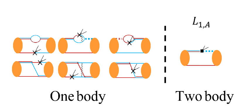
Figure 1: Different topologies of the diagrams contributing to the triton $\beta$-decay amplitude. The LHS of each diagram is ³H, while the RHS is ³He. The double lines are the propagators of the two dibaryon fields $D_{t}$ (solid), $D_{s}$ (dashed for $nn$ and $np$, dotted for $pp$), where the red (blue) lines denote a neutron (proton) propagator. Most of the diagrams couple both the triplet and the singlet channels. The diagrams with one-body interactions contribute to both $\langle||\text{F}||\rangle$ and $\langle||\text{GT}||\rangle$ transitions, while the two-body interactions are coupled to the effective ranges $\rho_{t}$ and $\rho_{s}$ and to $l_{1,A}$ ( and contribute only for the GT transition, where $L_{1,A}$ is defined in Eq. (9)).

The one-body diagrams that contain a one-body weak interaction contribute to both $\langle||\text{F}||\rangle$ and $\langle||\text{GT}||\rangle$ transitions. These one-body diagrams are taken up to NLO, and, therefore, contain the NLO insertion for the one-body diagrams, as discussed in Ref. De-Leon et al. (2019). The two-body diagrams include a two-body term originating from the ERE term in the Lagrangian, $\frac{1}{2}\frac{\rho_{t}+\rho_{s}}{\sqrt{\rho_{t}\rho_{s}}}g_{A}$, and the two-body operator whose coefficient is proportional to $l_{1,A}$. These diagrams contribute to the GT transition only.

V Numerical results

V.1 Fermi operator

In the absence of the Coulomb interaction, ³H is identical to ³He and the Fermi transition is equal to the triton wave function normalization as defined in Ref. De-Leon et al. (2019):

$$\langle||\text{F}||\rangle^{0}=\frac{\langle\psi^{{}^{3}\text{H}}\|{\tau}^{0}\|\psi^{{}^{3}\text{H}}\rangle}{\sqrt{2}}={\Bigl{\langle}\frac{1}{2}\Bigl{\|}\tau^{0}\Bigr{\|}\frac{1}{2}\Bigr{\rangle}}\\ \times\sum\limits_{\mu,\nu}{y_{\mu}y_{\nu}\psi^{{}^{3}\text{H}}_{\mu}(p^{\prime})\otimes}\left[d^{\prime ii}_{\mu\nu}\hat{\mathcal{I}}(0,0)\right.\\ \left.+a^{\prime ii}_{\mu\nu}\hat{\mathcal{K}}(0,0)\right]\otimes{\psi^{{}^{3}\text{H}}_{\nu}(p)}=1~{},$$ (33)

where in the absence of the Coulomb interaction:

$$d^{\prime ii}_{\mu,\nu} =\delta_{\mu,\nu}$$ (34)

$$a^{\prime ii}_{\mu\nu} =a_{\mu\nu}$$ (35)

From comparison between eqs. 19 and 20 with eqs. 31 and 32, we expect that $\langle||\text{F}||\rangle=1-\epsilon$ Schiavilla et al. (1998), where $\epsilon\ll 1$ originates mostly from the isospin breaking due to the Coulomb interaction. We can, therefore, examine the effects of isospin breaking on the Fermi transition due to the Coulomb interaction, and the additional one-photon exchange diagrams and then compare them to the Gamow-Teller transition. In this section, we present our calculations of the Fermi transition. First, we calculate the Fermi transition in the absence of the Coulomb interaction but under the assumption that $a_{nn,np}\neq a_{pp}$. Second, we calculate the Fermi transition with $\alpha\neq 0$, and, obviously, $a_{nn,np}\neq a_{pp}$, as a result, for both Z- and ERE-parameterization. All these calculations result from the LHS of the diagrams in Fig. 1.

We use the experimental data shown in Tab. 1 as input for our numerical calculations shown in Fig. 2 and Tab. 2.

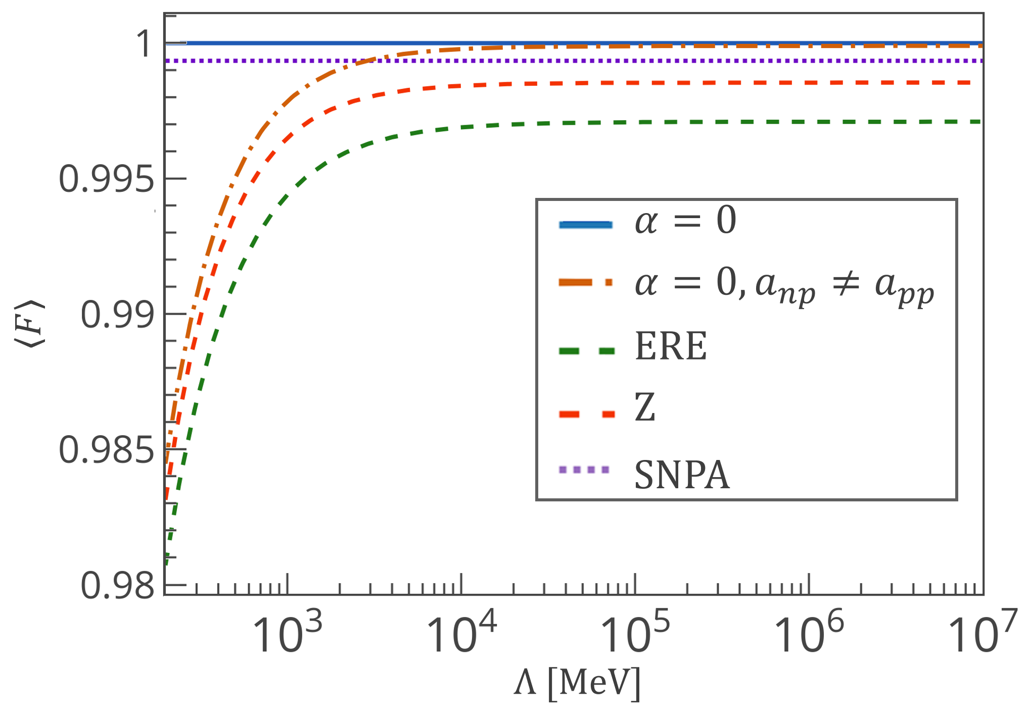
Figure 2: Numerical results of the Fermi transition. The solid line is the LO result of $\langle||\text{F}||\rangle=1$ with $\alpha=0$. The dashed-dotted line is the numerical result for $\alpha=0$ with isospin breaking effects in the scattering length: $a_{np}\neq a_{pp}$ (LO). The green (red) dashed line shows the numerical result at LO for the ERE- (Z-) parameterization with $\alpha\neq 0$. The dotted line is plotted at the value of $\langle||\text{F}||\rangle=0.9993$ from Ref. Schiavilla et al. (1998).

	$\langle||\text{F}||\rangle$
One-body, LO $\alpha=0$	1
One-body, LO $\alpha=0,a_{np}\neq a_{pp}$	0.9999
LO, ERE	0.9971
LO, Z	0.9985
SNPA Schiavilla et al. (1998)	0.9993

Table 2: Numerical results of $\langle||\text{F}||\rangle$. Note that the second row is without an explicit Coulomb force ($\alpha=0$) but with isospin breaking in the scattering lengths, i.e., with the physical values for the scattering lengths $a_{np}\neq a_{pp}$.

Our numerical result compares well to the $\langle||\text{F}||\rangle$ standard nuclear physics approach (SNPA) calculation by Schiavilla et al.  Schiavilla et al. (1998). The SNPA calculation involves nuclear wave functions derived from high-precision phenomenological nuclear potentials, one-nucleon, and two-nucleon electroweak currents.

V.2 Gamow-Teller operator

In contrast to the Fermi transition, the Gamow-Teller transition also involves two-body operators at NLO. The diagrams that contain a one-body weak interaction are coupled to $g_{A}$ and contain one ERE insertion up to NLO. The two-body diagrams are coupled to the two-body operators with prefactor $L_{1,A}$. By summing over all diagrams and comparing the resulting sum to the triton half-life, Chou et al. (1993), $l_{1,A}$ can be extracted, as will be discussed later in Section VI. We used the experimental input parameters shown in Tab. 1 for all numerical calculations.

We emphasize furthermore that in the absence of Coulomb interaction, the Fermi transition matrix element at LO is 1 (i.e., $\alpha=0$). Similarly, the LO matrix element of the Gamow-Teller transition with $\alpha=0$ was easily found to be:

$$\langle||\text{GT}||\rangle^{\text{LO}}_{\alpha=0}=\dfrac{\langle\frac{1}{2}\|\boldsymbol{\sigma}\|\frac{1}{2}\rangle}{\sqrt{2}}{\Bigl{\langle}\frac{1}{2}\Bigl{\|}\tau^{0}\Bigr{\|}\frac{1}{2}\Bigr{\rangle}}\\ \ \times\sum\limits_{\mu,\nu}y_{\mu}y_{\nu}{\psi^{{}^{3}\text{H}}_{\mu}(p^{\prime})\otimes}\left[\delta_{\mu,\nu}\hat{\mathcal{I}}(0,0)+a_{\mu\nu}\hat{\mathcal{K}}(0,0)\right]\otimes{\psi^{{}^{3}\text{H}}_{\nu}(p)}\\ =\dfrac{\sqrt{6}}{\sqrt{2}}=\sqrt{3}~{},$$ (36)

where $a_{\mu\nu}$ is given in eq. 19. We performed this calculation in two ways: one with $\alpha=0$ for both the scattering amplitude and the matrix element, and the other with $\alpha=0$ for the matrix element, but for different scattering lengths, similarly to the Fermi case. From Tab. 3, it is clear that the bulk of the Coulomb effect originates from the strong isospin breaking, i.e., different scattering lengths, and not from the explicit one-photon exchange diagrams. These results imply that for both the Fermi and Gamow-Teller transitions, the explicit Coulomb interaction, i.e., one-photon exchange diagrams, can be calculated perturbatively since their contribution to the matrix element is very small compared to the isospin breaking effect.

Our $\langle||\text{GT}||\rangle$ numerical results for both NLO arrangements are shown in Tab. 3 and in Fig. 3. The full NLO result with $l_{1,A}=0$ includes both one-body and two-body terms that contribute to $\langle||\text{GT}||\rangle$, without the diagrams that are coupled to $l_{1,A}$.

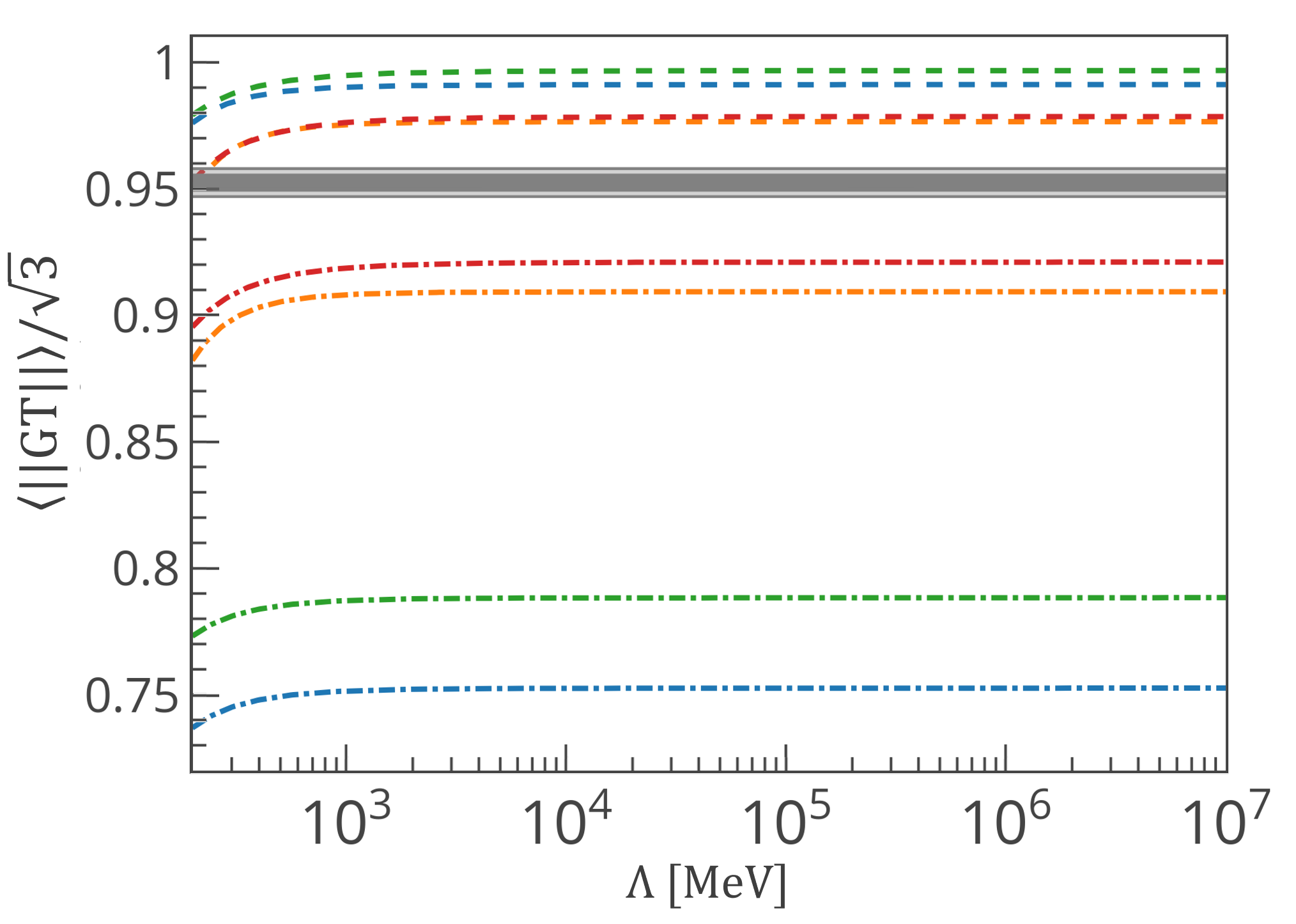
Figure 3: Numerical results of the Gamow-Teller transition. The gray area is the full $\langle||\text{GT}||\rangle$ matrix element with $g_{A}=1.273\pm 0.003\pm 0.005$ Olive and Group (2014); Morris et al. (2017). The blue (orange) short dashed line is the numerical result of $\langle||\text{GT}||\rangle^{\text{LO}}$ for the ERE- (Z-) parameterization, where $\alpha=0$ but $a_{np}\neq a_{pp}$. The green (red) short dashed line is the numerical result of $\langle||\text{GT}||\rangle^{\text{LO}}$ for the ERE- (Z-) parameterization, with $\alpha\neq 0$. The blue (orange) dashed-dotted line is $\langle||\text{GT}||\rangle^{\text{NLO}}$ result with $l_{1,A}=0$ for the ERE- (Z-) parameterization, where $\alpha=0$ but $a_{np}\neq a_{pp}$. The green (red) dashed-dotted line is $\langle||\text{GT}||\rangle^{\text{NLO}}$ result with $l_{1,A}=0$ and $\alpha\neq 0$, for the ERE- (Z-) parameterization.

	$\langle||\text{GT}||\rangle$, ERE	$\langle||\text{GT}||\rangle$, $Z$
One-body, LO $\alpha=0$	$\sqrt{3}$	$\sqrt{3}$
One-body, LO $\alpha=0$, $a_{np}\neq a_{pp}$	1.716	1.692
One-body, LO	1.727	1.695
Full NLO, $l_{1,A}=0$, $\alpha=0$, $a_{np}\neq a_{pp}$	1.301	1.575
Full NLO, $l_{1,A}=0$	1.383	1.596

Table 3: Numerical results for $\langle||\text{GT}||\rangle$. Note that the rows with the comment $``\alpha=0$, $a_{np}\neq a_{pp}$” are without an explicit Coulomb force ($\alpha=0$) but with isospin breaking in the scattering lengths, i.e., with physical values for the scattering lengths $a_{np}\neq a_{pp}$.

VI Extraction of the Gamow-Teller strength and fixing $l_{1,A}$

The GT matrix element can be extracted from the triton half-life calculation using Eq. (12). The axial coupling constant, $g_{A}$, has been remeasured recently, leading to results whose range is much bigger than the current recommendation. To be on the safe side, we take $g_{A}=1.273\pm 0.003\pm 0.005$ Morris et al. (2017); Olive and Group (2014). The first uncertainty in $g_{A}$ arises from the difference between the measurements of Refs. Olive and Group (2014); Morris et al. (2017), and the second uncertainty is the statistical experimental uncertainty. To extract the Gamow-Teller strength, we use our prediction for the Fermi transition: $\langle\text{F}\rangle=0.9993$ Schiavilla et al. (1998). At large cutoff values, we find the empirical GT strength to be $\langle||\text{GT}||\rangle_{\text{emp}}=\sqrt{3}\frac{1.213\pm 0.002}{g_{A}}$ Schiavilla et al. (1998). The uncertainty here originates mainly from the uncertainty in the triton half-life.

The difference between the empirical GT strength and the numerical result for the GT-transition at NLO is used to fix $l_{1,A}$ such that:

$$\l_{1,A}(\Lambda)=\frac{\langle||\text{GT}||\rangle_{\text{emp}}-\langle||\text{GT}||\rangle_{l_{1,A}=0}^{\text{NLO}}}{\langle||\text{GT}||\rangle_{l_{1,A}}^{\text{NLO}}}~{},$$ (37)

where $\langle||\text{GT}||\rangle_{l_{1,A}}^{\text{NLO}}$ are the two-body diagrams that contribute to the triton $\beta$-decay and are coupled to $l_{1,A}$, while $\langle||\text{GT}||\rangle_{l_{1,A}=0}^{\text{NLO}}$ is the sum over all the diagrams that contribute to the triton $\beta$-decay without the diagrams coupled to $l_{1,A}$. The numerical results for $l_{1,A}$ for both ERE- and $Z$-parameterizations are shown in Fig. 4.

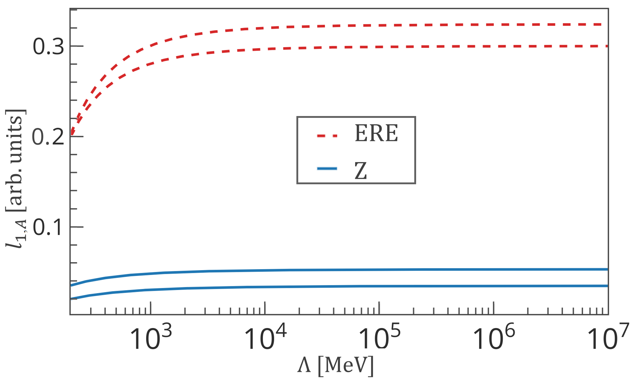
Figure 4: Numerical results of $l_{1,A}$, with $g_{A}=1.273\pm 0.003\pm 0.005$ Olive and Group (2014); Morris et al. (2017). The dashed (solid) lines are the upper and lower limits of the calculations in ERE- (Z-) parameterization.

Importantly, we find numerically, that for both parameterizations, $l_{1,A}$ converges with increasing UV cutoff, a fact that has been already predicted by theory Butler and Chen (2000), where:

$$l_{1,A}^{\text{ERE}} =0.312\pm 0.004\pm 0.004\pm 0.001$$ (38a)

$$l_{1,A}^{\text{Z}} =0.051\pm 0.004\pm 0.004\pm 0.001~{},$$ (38b)

The first and second uncertainties come from the aforementioned difference between recent experimental determinations of $g_{A}$ and $g_{A}$ statistical uncertainties Olive and Group (2014); Morris et al. (2017) while the third uncertainty comes from the rest of the experimental uncertainties, such as the statistical uncertainties in the measured triton half-life.

VII Previous extractions of $l_{1,A}$

Due to the importance of $l_{1,A}$, as the first two-body LEC that appears in the pionless description of $pp$-fusion, its determination has attracted much attention in the literature. In this subsection, we review previous extractions of $l_{1,A}$ in the $\pi\text{/}$EFT and the latest predictions of the $pp$-fusion rate.

Two main approaches were taken in previous studies to determine $l_{1,A}$. In the first, an experimental value of a two-body weak interaction process, usually at the cutoff $\mu=m_{\pi}$, was used for matching. Among these reactions are the deuteron dissociation by anti-neutrinos from reactors M. et al. (2002) and neutrino reactions with the deuteron, as measured in SNO Chen et al. (2003). Both references extract $L^{\prime}_{1,A}$ as defined in Eq. (8) as $4.0\pm 6.3$ (Ref. M. et al. (2002)) and $3.6\pm 4.6$ (Ref. Chen et al. (2003)). Using Eq. (10) and $\mu=m_{\pi}$ we can extract $l_{1,A}=0.09\pm 0.14$ and $l_{1,A}=0.08\pm 0.11$, respectively.

In both cases, the large uncertainties originate from statistical errors in the experiments, due to the small cross-section for neutrino-deuteron reactions. The authors of Ref. Chen et al. (2005) proposed, therefore, a precision measurement of muon capture on the deuteron, with the aim of reducing the uncertainties by a factor of 3, reflecting an estimated 2-3% experimental uncertainty in the (then proposed) ongoing MuSun experiment Andreev et al. (2010). It is important to note that the $\mu^{-}d$ capture has a large energy transfer, possibly too large for an application of $\pi\text{/}$EFT . In all these studies, the uncertainties are mainly experimental, due to the uncertainty in the observable, , i.e., neglecting the truncation error.

A different approach was taken by Ando and collaborators in Ref. Ando et al. (2008). They used the hybrid calculation of the $pp$-fusion rate from Park et al. Park et al. (2003). The authors took the ratio of the two-body strength over the one-body strength was taken from this calculation and fixed $L_{1,A}$ to reproduce this ratio in the $\pi\text{/}$EFT regime. Ando et al. defined the coefficient of the two-body counterterm as $L_{1,A}=-\left(g_{A}\frac{\rho_{s}+\rho_{t}}{2\sqrt{\rho_{s}\rho_{t}}}+\frac{l_{1,A}^{\rm Ando}}{M\sqrt{\rho_{s}\rho_{t}}}\right)$. Using the value $l^{\rm Ando}_{1,A}=-0.5\pm 0.03$, we find $l_{1,A}=0.038\pm 0.002$. The small uncertainty in this result is due to the accurate triton half-life measurement that is used to fix the undetermined counterterms in Ref. Park et al. (2003). However, this work has been criticized since it is not guaranteed that their approach is consistent. It employs two very different models and non-observable quantities to perform the matching.

In 2017, The Nuclear Physics with Lattice Quantum Chromo Dynamics (NPLQCD) collaboration calibrated $L_{1,A}$ using the triton $\beta$-decay Savage et al. (2017) for the non-physical pion mass $m_{\pi}=805\,\text{MeV}$ and then extrapolated it to the physical pion mass.

VIII Summary and outlook

In this paper, we have used the approach introduced in Ref. De-Leon et al. (2019) to study tritium $\beta$-decay in the framework of pionless effective field theory at next-to-leading order (NLO). The EFT approach used here is useful for robust and reliable theoretical uncertainty estimates, based on neglected orders in the EFT expansion. The results presented in this paper show that tritium $\beta$-decay can be calculated reliably, that the corresponding matrix elements are properly renormalized and that the half-life displays, therefore, the necessary RG invariance at NLO.

We found furthermore that up to NLO, the Coulomb interaction i.e., the one-photon exchange interaction, can be included perturbatively in the calculation of this observable, which is consistent with its effect on the ³He binding energy as already discussed in Refs. König and Hammer (2011); König et al. (2015, 2016); De-Leon et al. (2019).

Tritium $\beta$-decay depends on two matrix elements, the Fermi transition, which includes a one-body polar-vector part, and the Gamow-Teller transition, which includes one- and two-body axial-vector parts.

We have tested the correct renormalization of our perturbative calculation of the Fermi and Gamow-Teller matrix elements with an analysis of the residual cutoff dependence at cutoffs that are significantly larger than the breakdown scale of the EFT.

We have used the NLO calculation to fix the NLO LEC, $l_{1,A}$ that is needed for a high-accuracy prediction of the solar proton-proton fusion rate Kong and Ravndal (1999a, 2001); Ando et al. (2008). The NLO correction that originates from the $l_{1,A}$ counterterm (short-range corrections) is about 3% (15%) of the tritium decay Gamow-Teller strength in the Z-(ERE-) parameterization. The short-range corrections associated with the ERE-parameterization are significantly larger than those associated with the Z-parameterization, which implies that the ERE-parameterization internal error is larger than that of the Z-parameterization. Also, the fact that our calculation is carried out within a consistent perturbative approach allows reliable uncertainty estimates originating from the experimental uncertainties in $g_{A}$ and the half-life measurement.

Knowledge of $l_{1,A}$ is required for higher-order calculations of a number of weak processes, such as $pp$-fusion Adelberger et al. (1998); Kong and Ravndal (1999a, 2001); Ando et al. (2008) and muon capture Chen et al. (2005); Marcucci and Piarulli (2011); Ackerbauer et al. (1998); Gazit (2009, 2008). In the near future, we intend to examine our result for $l_{1,A}$, and its uncertainty by addressing these low-energy weak processes Marcucci et al. (2013); Acharya et al. (2016) when theoretical and empirical uncertainties estimations must accompany this prediction. Besides, the calibration of LEC from a ³H $\beta$-decay for the prediction of a two-nucleon process (such as $pp$-fusion) is based on the assumption that $\pi\text{/}$EFT is the appropriate framework for calculating observables in the $A=2$ and $A=3$ systems. However, this consistency cannot be examined using the weak observables only due to the small number of appropriate reactions. Hence, another set of well-measured low-energy $A<4$ interactions with similar characteristics to those of the weak reactions is needed for validation and verification of $\pi\text{/}$EFT . The strong analogy between the electromagnetic to weak observables indicates that well-measured electromagnetic observables can serve as the required candidates. We intend to use our perturbative framework for calculating general matrix element that can predict the low-energy electromagnetic $A<4$ observables. These observables can serve as a case study for estimating the theoretical uncertainty of $\pi\text{/}$EFT and LEC extractions from the $A<4$ observables predictions De-Leon and Gazit (2019).

References

- Bedaque and van Kolck (2002) P. F. Bedaque and U. van Kolck, “Effective field theory for few nucleon systems,” Ann. Rev. Nucl. Part. Sci. 52, 339–396 (2002).
- Kaplan et al. (1996) D. B. Kaplan, M. J. Savage, and M. B. Wise, “Nucleon - nucleon scattering from effective field theory,” Nucl. Phys. B478, 629–659 (1996).
- Kaplan et al. (1998a) D. B. Kaplan, M. J. Savage, and M. B. Wise, “Two nucleon systems from effective field theory,” Nucl. Phys. B534, 329–355 (1998a).
- Kaplan et al. (1998b) D. B. Kaplan, M. J. Savage, and M. B. Wise, “A New expansion for nucleon-nucleon interactions,” Phys. Lett. B424, 390–396 (1998b).
- Kaplan et al. (1999) D. B. Kaplan, M. J. Savage, and M. B. Wise, “A Perturbative calculation of the electromagnetic form-factors of the deuteron,” Phys. Rev. C59, 617–629 (1999).
- GriessHammer (2005) H. W. GriessHammer, “Naive dimensional analysis for three-body forces without pions,” Nucl. Phys. A760, 110–138 (2005).
- Platter (2009) L. Platter, “Low-Energy Universality in Atomic, and Nuclear Physics,” Few Body Syst. 46, 139–171 (2009).
- König and Hammer (2011) S. König and H.-W. Hammer, “Low-energy scattering, and 3He in pionless EFT,” Phys. Rev. C83, 064001 (2011).
- König et al. (2015) S. König, H. W. GriessHammer, and H. W. Hammer, “The proton-deuteron system in pionless EFT revisited,” J. Phys. G42, 045101 (2015).
- König et al. (2016) S. König, H. W. GriessHammer, H.-W. Hammer, and U. van Kolck, “Effective theory of 3H, and 3He,” J. Phys. G43, 055106 (2016).
- De-Leon et al. (2019) H. De-Leon, L. Platter, and D. Gazit, “Calculation of bound state matrix element in pionless effective field theory,” (2019), arXiv:1902.07677 [nucl-th] .
- Ando and Birse (2010) S.-I Ando and M. C. Birse, “Effective field theory of 3He,” J. Phys. G37, 105108 (2010).
- Gautam and Kong (2003) R. Gautam and X.-W. Kong, “Quartet S wave p d scattering in EFT,” Nucl. Phys. A717, 73–90 (2003).
- Vanasse et al. (2014) J. Vanasse, D. A. Egolf, J. Kerin, S. König, and R. P. Springer, “ and Scattering to Next-to-Leading Order in Pionless Effective Field Theory,” Phys. Rev. C89, 064003 (2014).
- Adelberger et al. (2011) E. G. Adelberger et al., “Solar fusion cross sections II: the pp chain, and CNO cycles,” Rev. Mod. Phys. 83, 195 (2011).
- Schiavilla et al. (1998) R. Schiavilla, V. G. J. Stoks, W. Glöckle, H. Kamada, A. Nogga, J. Carlson, R. Machleidt, V. R. Pandharipande, R. B. Wiringa, A. Kievsky, S. Rosati, and M. Viviani, “Weak capture of protons by protons,” Phys. Rev. C 58, 1263–1277 (1998).
- Gazit et al. (2009) D. Gazit, S. Quaglioni, and P. Navrátil, “Three-nucleon low-energy constants from the consistency of interactions, and currents in chiral effective field theory,” Phys. Rev. Lett. 103, 102502 (2009).
- Park et al. (2003) T.-S. Park, L. E. Marcucci, R. Schiavilla, M. Viviani, A. Kievsky, S. Rosati, K. Kubodera, D.-P. Min, and M. Rho, “Parameter-free effective field theory calculation for the solar proton-fusion, and hep processes,” Phys. Rev. C 67, 055206 (2003).
- Kong and Ravndal (1999a) X. Kong and F. Ravndal, “Proton proton fusion in leading order of effective field theory,” Nucl. Phys. A656, 421–429 (1999a).
- Kong and Ravndal (2001) X. Kong and F. Ravndal, “Proton proton fusion in effective field theory,” Phys. Rev. C64, 044002 (2001).
- Butler and Chen (2000) M. Butler and J.-W. Chen, “Elastic, and inelastic neutrino deuteron scattering in effective field theory,” Nucl. Phys. A675, 575–600 (2000).
- Butler and Chen (2001) M. Butler and J.-W. Chen, “Proton proton fusion in effective field theory to fifth order,” Phys. Lett. B520, 87–91 (2001).
- Chen et al. (2005) J.-W. Chen, T. Inoue, X.-D. Ji, and Y. Li, “Fixing two-nucleon weak-axial coupling L(1,A) from mu- d capture,” Phys. Rev. C72, 061001 (2005).
- Ando et al. (2008) S. Ando, J. W. Shin, C. H. Hyun, S. W. Hong, and K. Kubodera, “Proton-proton fusion in pionless effective theory,” Phys. Lett. B668, 187–192 (2008).
- Beane and Savage (2001) S. R. Beane and M. J. Savage, “Rearranging pionless effective field theory,” Nucl. Phys. A694, 511–524 (2001).
- Phillips et al. (2000) D. R. Phillips, G. Rupak, and M. J. Savage, “Improving the convergence of N N effective field theory,” Phys. Lett. B473, 209–218 (2000).
- Van Der Leun and Alderliesten (1982) C. Van Der Leun and C. Alderliesten, “The deuteron binding energy,” Nucl. Phys. A380, 261–269 (1982).
- de Swart et al. (1995) J. J. de Swart, C. P. F. Terheggen, and V. G. J. Stoks, “The Low-energy n p scattering parameters, and the deuteron,” in 3rd International Symposium on Dubna Deuteron 95 Dubna, Russia, July 4-7, 1995 (1995).
- (29) M. A. Preston and R. K Bhaduri, “Structure of the nucleus,” .
- Bergervoet et al. (1988) J. R. Bergervoet, P. C. van Campen, W. A. van der Sanden, and Johan J. de Swart, “Phase shift analysis of 0-30 MeV pp scattering data,” Phys. Rev. C38, 15–50 (1988).
- GriessHammer (2004) H. W. GriessHammer, “Improved convergence in the three-nucleon system at very low energies,” Nucl. Phys. A744, 192–226 (2004).
- Vanasse (2013) J. Vanasse, “Fully Perturbative Calculation of Scattering to Next-to-next-to-leading-order,” Phys. Rev. C88, 044001 (2013).
- J. (2017) Vanasse J., “Triton charge radius to next-to-next-to-leading order in pionless effective field theory,” Phys. Rev. C95, 024002 (2017).
- Faddeev and Merkuriev (1993) L.D. Faddeev and S.P. Merkuriev, Quantum Scattering Theory for Several Particle Systems (Springer, 1993).
- Bedaque et al. (1999) P. F. Bedaque, H.-W. Hammer, and U. van Kolck, “The Three boson system with short range interactions,” Nucl. Phys. A646, 444–466 (1999).
- Bedaque et al. (2000) P. F. Bedaque, H.-W. Hammer, and U. van Kolck, “Effective theory of the triton,” Nucl. Phys. A676, 357–370 (2000).
- Kong and Ravndal (2000) X. Kong and F. Ravndal, “Coulomb effects in low-energy proton proton scattering,” Nucl. Phys. A665, 137–163 (2000).
- Kong and Ravndal (1999b) X. Kong and F. Ravndal, “Proton proton scattering lengths from effective field theory,” Phys. Lett. B450, 320–324 (1999b).
- Kirscher and Gazit (2016) J. Kirscher and D. Gazit, “The Coulomb interaction in Helium-3: Interplay of strong short-range, and weak long-range potentials,” Phys. Lett. B755, 253–260 (2016).
- Akulov and Mamyrin (2005) Yu. A. Akulov and B. A. Mamyrin, “Half-life, and fT1/2 value for the bare triton,” Phys. Lett. B610, 45–49 (2005).
- Hardy et al. (1990) J. C. Hardy, I. S. Towner, V. T. Koslowsky, E. Hagberg, and H. Schmeing, “Superallowed nuclear beta decays: a Critical survey with tests of CVC, and the standard model,” Nucl. Phys. A509, 429–460 (1990).
- Simpson (1987) J. J. Simpson, “Half-life of tritium, and the Gamow-Teller transition rate,” Phys. Rev. C35, 752–754 (1987).
- GriessHammer et al. (2012) H. W. GriessHammer, M. R. Schindler, and R. P. Springer, “Parity-violating neutron spin rotation in hydrogen, and deuterium,” Eur. Phys. J. A48, 7 (2012).
- Chou et al. (1993) W. T. Chou, E. K. Warburton, and B. A. Brown, “Gamow-Teller beta-decay rates for nuclei,” Phys. Rev. C47, 163–177 (1993).
- Olive and Group (2014) K. A. Olive and Particle Data Group, “Review of particle physics,” Chinese Physics C 38, 090001 (2014).
- Morris et al. (2017) C. L. Morris et al., “A new method for measuring the neutron lifetime using an in situ neutron detector,” Review of Scientific Instruments 88, 053508 (2017).
- M. et al. (2002) Butler M., Chen J.-W., and Vogel P., “Constraints on two-body axial currents from reactor anti-neutrino deuteron breakup reactions,” Phys. Lett. B549, 26–31 (2002).
- Chen et al. (2003) J.-W. Chen, Karsten. H., M., and R. G. Hamish Robertson, “Constraining the leading weak axial two-body current by recent solar neutrino flux data,” Phys. Rev. C 67, 025801 (2003).
- Andreev et al. (2010) V. A. Andreev et al. (MuSun), “Muon Capture on the Deuteron – The MuSun Experiment,” (2010), arXiv:1004.1754 [nucl-ex] .
- Savage et al. (2017) M. J. Savage, P. E. Shanahan, B. C. Tiburzi, M. L. Wagman, F. Winter, S. R. Beane, E. Chang, Z. Davoudi, W. Detmold, and K. Orginos (NPLQCD Collaboration), “Proton-proton fusion, and tritium decay from lattice quantum chromodynamics,” Phys. Rev. Lett. 119, 062002 (2017).
- Adelberger et al. (1998) E. G. Adelberger et al., “Solar fusion cross-sections,” Rev. Mod. Phys. 70, 1265–1292 (1998).
- Marcucci and Piarulli (2011) L. E. Marcucci and M. Piarulli, “Muon capture on light nuclei,” International Workshop on Relativistic Description of Two- and Three-body Systems in Nuclear Physics Trento, Italy, October 19-23, 2009, Few Body Syst. 49, 35–39 (2011).
- Ackerbauer et al. (1998) P. Ackerbauer et al., “A precision measurement of nuclear muon capture on 3He,” Phys. Lett. B417, 224–232 (1998).
- Gazit (2009) D. Gazit, “The Weak structure of the nucleon from muon capture on 3He,” Particles, and nuclei. Proceedings, 18th International Conference, PANIC08, Eilat, Israel, November 9-14, 2008, Nucl. Phys. A827, 408C–410C (2009).
- Gazit (2008) D. Gazit, “Muon Capture on 3He, and the Weak Structure of the Nucleon,” Phys. Lett. B666, 472–476 (2008).
- Marcucci et al. (2013) L. E. Marcucci, R. Schiavilla, and M. Viviani, “Proton-proton weak capture in chiral effective field theory,” Phys. Rev. Lett. 110, 192503 (2013).
- Acharya et al. (2016) B. Acharya, B.D. Carlsson, A. Ekström, C. Forssén, and L. Platter, “Uncertainty quantification for proton-proton fusion in chiral effective field theory ,” Physics Letters B 760, 584 – 589 (2016).
- De-Leon and Gazit (2019) H. De-Leon and D. Gazit, “Precise, and accurate calculation of low energy magnetic reactions in nuclear systems using effective field theory without pions,” In preparation (2019).