An algorithm based on a new DQM with modified exponential cubic B-splines for solving hyperbolic telegraph equation in dimension
Abstract
This paper developed a method called ”modified exponential cubic B-Spline differential quadrature (mExp-DQM) for space discretization together with a time integration algorithm” for the numerical computation of hyperbolic telegraph equation in dimension. The mExp-DQM is a new differential quadrature method based on modified exponential cubic B-splines as basis which reduces the problem into an amenable system of ordinary differential equations. The resulting system is solved using a time integration algorithm. The stability of the method is also studied by computing the eigenvalues of the coefficients matrices, it is found that the scheme is conditionally stable. The accuracy of the method is illustrated by computing the error between analytical solutions and numerical solutions is measured by using and error norms for each problem. A comparison of mExp-DQM solutions with the results of the other numerical methods has been carried out for various space sizes and time step sizes.
Keywords: Differential quadrature method, hyperbolic telegraph equation, modified exponential cubic B-splines, mExp-DQM, Thomas algorithm.
1 Introduction
The hyperbolic partial differential equations have a great attention due to its wide range of applications in fields of applied science and engineering, for instance, the hyperbolic partial differential equation models fundamental equations in atomic physics [1] and is very useful in understanding various physical phenomena in applied sciences and engineering. It models the vibrations of structures (e.g. buildings, machines and beams). We consider second-order two-space dimensional linear hyperbolic telegraph equation of the form:
| (1) |
where denotes the boundary of the computational domain and are arbitrary constants. Eq. (1) with is a damped wave equation while for it reduces to telegraph equation. The telegraph equation is more convenient than ordinary diffusion equation in modeling reaction diffusion for such branches of sciences [2], and mostly used in wave propagation of electric signals in a cable transmission line [3].
Two space dimensional initial boundary value problem for second order linear telegraph equation (1) is obtained by combining the equation with the following initial conditions:
| (2) |
and the boundary conditions- Dirichlet boundary condition:
| (3) |
or Neumann boundary conditions:
| (4) |
where are known smooth functions.
In the recent years, a lot of numerical techniques have been developed for solving hyperbolic telegraph equations in both one and two dimensions, among them: Taylor matrix method [4], dual reciprocity boundary integral method [2], unconditionally stable finite difference scheme [5], implicit difference scheme [8], variational iteration method [9],modified B-spline collocation method [6], Chebyshev tau method [7], interpolating scaling function method [1], cubic B-spline collocation method [10].
Two dimensional initial value problem of telegraph equation have been solved by various schemes: Taylor matrix method by Bülbül and Sezer [11] which converts the telegraph equation into the matrix equation, Two meshless methods- namely meshless local weak-strong (MLWS) and meshless local Petrov-Galerkin (MLPG) method by Dehghan and Ghesmati [12], higher order implicit collocation method [13], A polynomial based differential quadrature method [14], modified cubic B-spline differential quadrature method [27], an unconditionally stable alternating direction implicit scheme [18], A hybrid method due to Dehghan and Salehi [15], compact finite difference scheme by Ding and Zhang [16] with accuracy of order four in both space and time. Two dimensional linear hyperbolic telegraph equation with variable coefficients has been solved by Dehghan and Shorki [17].
In the recent years, the differential quadrature method (DQM), developed by Bellman et al. [20, 21] for the numerical computation of partial differential equations (PDEs), have a great attention among the researchers. After seminal work of Bellman et al.[20, 21], Quan and Chang [22, 23], the DQM has been employed with various types of basis functions, among others, cubic B-spline DQM [24, 25], modified cubic B-spline differential quadrature method (MCB-DQM) [26, 27], DQM based on fourier expansion and Harmonic function [28, 29, 30], sinc differential quadrature method [31], generalized DQM [32], polynomial based DQM [35, 14], quartic B-spline based DQM [36], Quartic and quintic B-spline methods [37], exponential cubic B-spline DQM [38], extended cubic B-spline DQM [39].
In this paper our aim is to develop modified exponential cubic-B-spline differential quadrature method (mExp-DQM) for hyperbolic partial differential equations. Specially, mExp-DQM is employed for the numerical computation of two dimensional second order linear hyperbolic telegraph equation with both Dirichlet boundary conditions and Neumann boundary conditions. The mExp-DQM is the differential quadrature method based on modified exponential cubic-B-splines as set of new basis functions. The mExp-DQM converts the initial- boundary value system of the telegraph equation into a initial value system of ODEs, in time. The resulting system of ODEs can be solved by using various time integration algorithm, among them, we prefer SSP-RK54 scheme [41, 42] due to its reduce storage space, results in less accumulation of the numerical errors. The accuracy and adaptability of the method is illustrated by considering six test problems of the two dimensional telegraphic equations.
The rest of the paper is organized into five more sections, which follow this introduction. Specifically, Section 2 deals with the description of mExp-DQM. Section 3 is devoted to the procedure for the implementation of mExp-DQM for the problem (1) with the initial conditions (2) and boundary conditions (3) and (4). The stability analysis of the mExp-DQM is studied in Section 4. Section 5 is concerned with the main aim, the numerical study of six test problems, to establish the accuracy of the proposed method in terms of the relative error norm (), and error norms. Finally, Section 6 concludes the paper with reference to critical analysis and research perspectives.
2 Description of mExp-DQM
The differential quadrature method is an approximation to derivatives of a function is the weighted sum of the functional values at certain nodes [21]. The weighting coefficients of the derivatives is depend only on grids [32]. This is the reason for taking the partitions of the computational domain of the problem is distributed uniformly as follows:
where , and are the discretization steps in both and directions, respectively. That is, a uniform partition in each -direction with the following grid points:
Let be the generic grid point and
The approximation for -th order derivative of , for , with respect to at for is given by
| (5) |
where the coefficients and , the time dependent unknown quantities, are termed as the weighting functions of the th-order derivative, to be calculated using of various type of basis functions.
The exponential cubic B-splines function at node in direction, reads [38, 19]:
| (11) |
where
The set forms a basis over the interval . The values of and its first and second derivatives in the grid point , denoted by , and , respectively, read:
| (15) | |||
| (19) | |||
| (23) |
The modified exponential cubic B-splines basis functions are obtained by modifying the exponential cubic B-spline basis function (11) as follows [26]:
| (24) |
The set is a basis over the set . Analogously procedure is followed for direction.
2.1 The evaluation of the weighting coefficients and
In order to evaluate the weighting coefficients of first order partial derivative in Eq. (5), we use the modified exponential cubic B-spline , in DQ method as set of basis functions. Write and , In DQ method, the approximate values of the first-order derivative is obtained as:
| (25) |
Setting , (the unknown weighting coefficient matrix), and , then Eq. (25) can be re-written as the following set of system of linear equations:
| (26) |
Let and , then the coefficient matrix of order can be obtained from (15) and (24):
and in particular the columns of the matrix read:
It is remarked that the exponential cubic B-splines are modified in order to have a diagonally dominant coefficient matrix , see Eq. (26). To calculate the weighting coefficients, we solve the system (26) using the well known Thomas Algorithm [40]. Similarly, the weighting coefficients can be evaluated by considering the grids in the direction.
In similar manner, the weighting coefficients and , for , can be calculated using the weighting functions in quadrature formula for second order derivative on the given basis functions. But, in the present paper, we prefer the following recursive formulae [32]:
| (27) |
3 The mExp-DQM for the telegraph equation
First, we set and thus . Keeping all above in mind, the second order telegraph equation (1) with the initial condition transforms to initial valued coupled system of first order differential equations as follows:
| (28) |
Further, on setting , the mExp-DQM transforms Equation (28) to
| (29) |
Next, further simplification is not required in case of Dirichlet boundary conditions. In this case the solution on the boundary can be read directly from the conditions (3) as:
| (30) |
But, for Neumann or mixed type boundary conditions, further simplification is required. In this case, the solutions at the boundary are obtained by using mExp-DQM on the boundary. This yields a system of linear equations, and on solving resulting system of the linear, the desired solution is obtained at the boundaries.
In particular, Eq. (5) with and the Neumann boundary conditions (4) at and can be written as
| (31) |
In terms of matrix system for , the above equation can be rewritten as
| (32) |
where and .
On solving (32), we have
| (33) |
On solving the above system of equations for the boundary values and , we have
| (34) |
Finally, on using boundary values and obtained from either boundary conditions (Dirichlet boundary conditions (3) or Neumann boundary conditions (4)), Eq. (29) can be rewritten as follows:
| (35) |
where and
| (36) |
A lot time integration schemes have been proposed for the numerical computation of initial valued system of differential equations (35), among others, the SSP-RK scheme allows low storage and large region of absolute property [41, 42]. In what follows, we adopt SSP-RK54 scheme, is strongly stable for nonlinear hyperbolic differential equations:
4 Stability analysis
In compact form , the system (35) can be rewritten as follows:
| (37) |
where
-
, and
-
and are null matrices;
-
is the identity matrix of order ;
-
the vector solution at the grid points:
.
.
-
, where , for is calculated from Eq. (36).
-
, where and are the following matrices (of order ) of the weighting coefficients and :
(38) where identity matrix, , and null matrix, , both are of order and
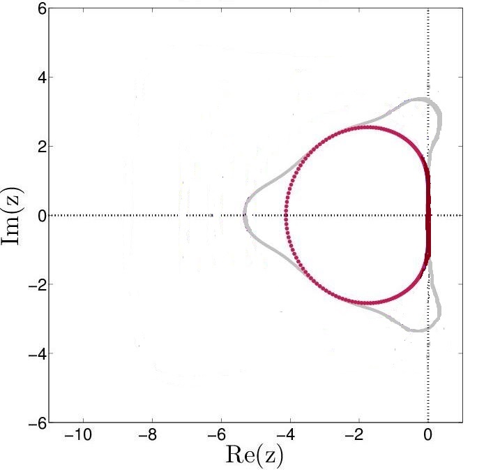
The stability of mExp-DQM for the telegraph equation (1) depends on the stability of the system of ODEs defined in (37). It is to be noticed that whenever the system of ODEs (37) is unstable, the proposed method for temporal discretization may not converge to the exact solution. Moreover, being the exact solution can directly obtained by means of the eigenvalues method, the stability of (37) depends on the eigenvalues of the coefficient matrix [43]. In fact, the stability region is the set , where is the stability function and is the eigenvalue of the coefficient matrix . For SSP-RK54 scheme the stability region is depicted in Fig 2, see [44, Fig. 5]. This evident that the sufficient condition for the stability of the system (37) is that to each eigenvalue of the coefficient matrix A, , and hence, the real part of each eigenvalue is necessarily either zero or negative.
Let be an eigenvalue of associated with the eigenvector , where each component is a vector of order . Then from Eq. (37) we have
| (39) |
which yields
| (40) |
and
| (41) |
Simplifying Eq. (40) and Eq. (41), we get
| (42) |
which confirms that the eigenvalue of is . By definition the matrix is:
| (43) |
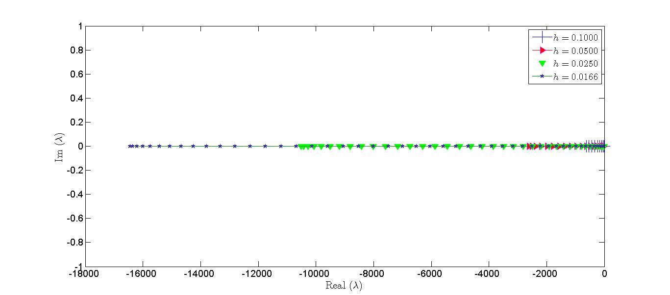
Now, we compute the eigenvalues of for and different grid sizes: , and depicted in Fig 2.
It is evident from Eq. (43) and Fig. 2 that for different values of the grid sizes the computed eigenvalues of are real negative numbers, that is
| (44) |
where and denote the real and the imaginary part of , respectively.
Let , then
| (45) |
According to Eq. (44) and Eq. (45), we have
| (46) |
The possible solutions of Eq.(46) are
-
If , then
-
If , then
In each case is negative whenever . One a given grid size, one can find a sufficient small value of so that , for each eigenvalue of matrix , lie inside the stability region of SSP-RK54 scheme. This shows that the mExp-DQM produces stable solutions for two dimensional second order linear telegraph equation.
5 Numerical experiments and discussion
This section with the main goal of the paper, the computation of numerical solution of the telegraph equation. The accuracy and the efficiency of this method is measured for six numerical examples in terms of the discrete relative error , and error norms:
where represent the numerical solution at node . Throughout the section, we have taken equal grid size in each direction, i.e., .
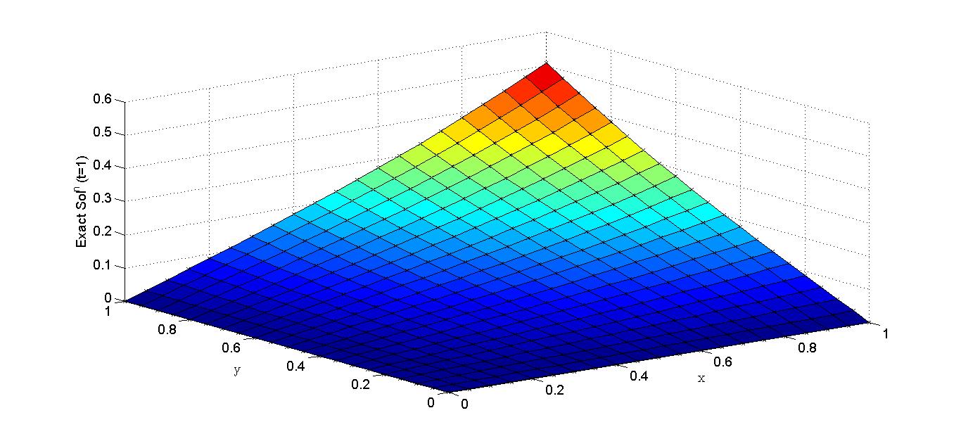
Example 1
Consider the telegraph equation (1) in the region with , , , and the Dirichlet boundary conditions:
| (47) |
The exact solution [2] is
| (48) |
The computed relative error (), error norms are compared with the recent results of Mittal and Bhatia [27] at different time levels , reported in Table 1 and Table 2 with the parameters and and , respectively.
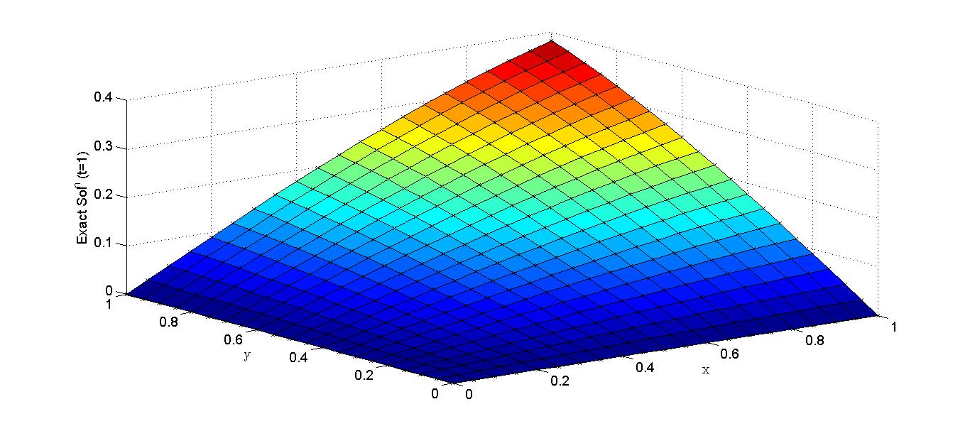
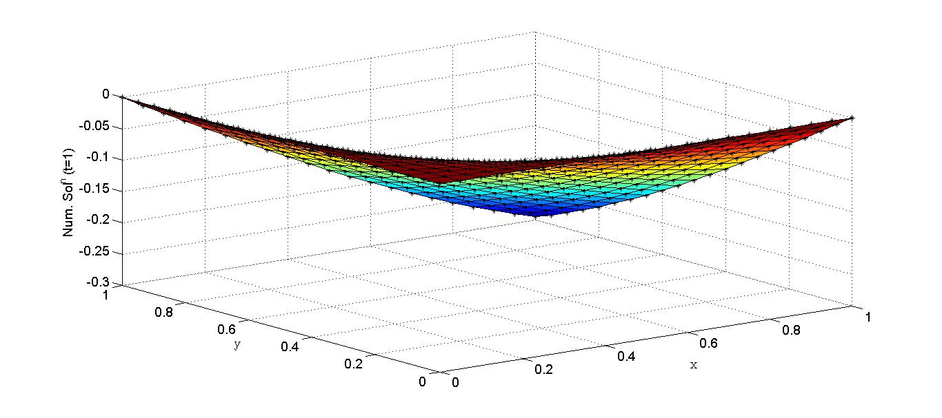
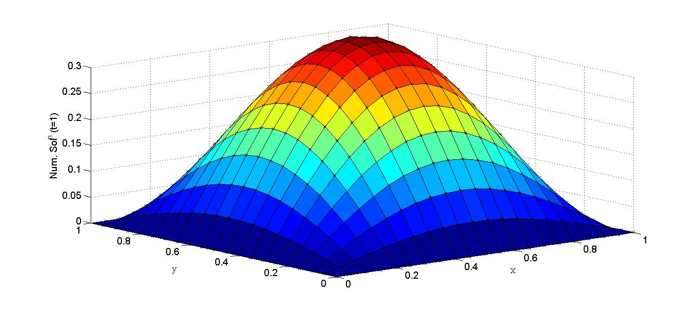
The comparison of computed physical solution behavior with the the exact solution behavior at is depicted in Fig. 3 with . The findings shows that the proposed solution are much better than that of Mittal and Bhatia[27], and are in excellent agreement with the exact solutions. The computation time is slightly more than Mittal and Bhatia[27] for large due to selection of SSP-RK54 scheme instead of SSP-RK43 scheme in time integration.
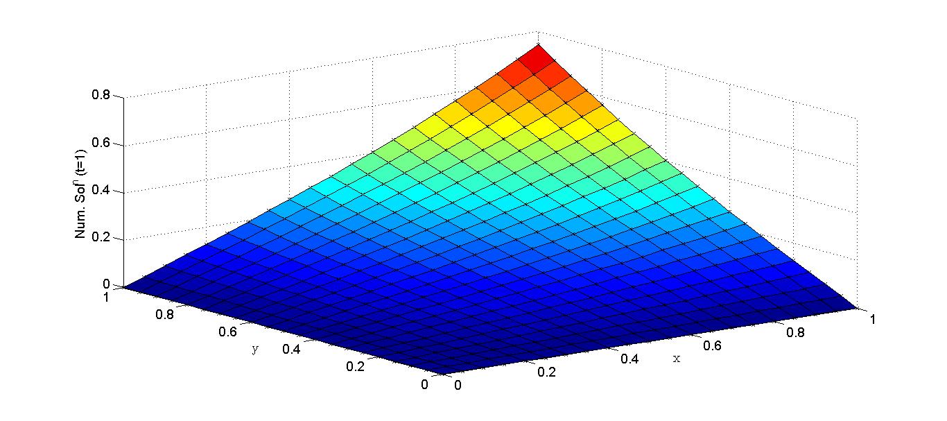
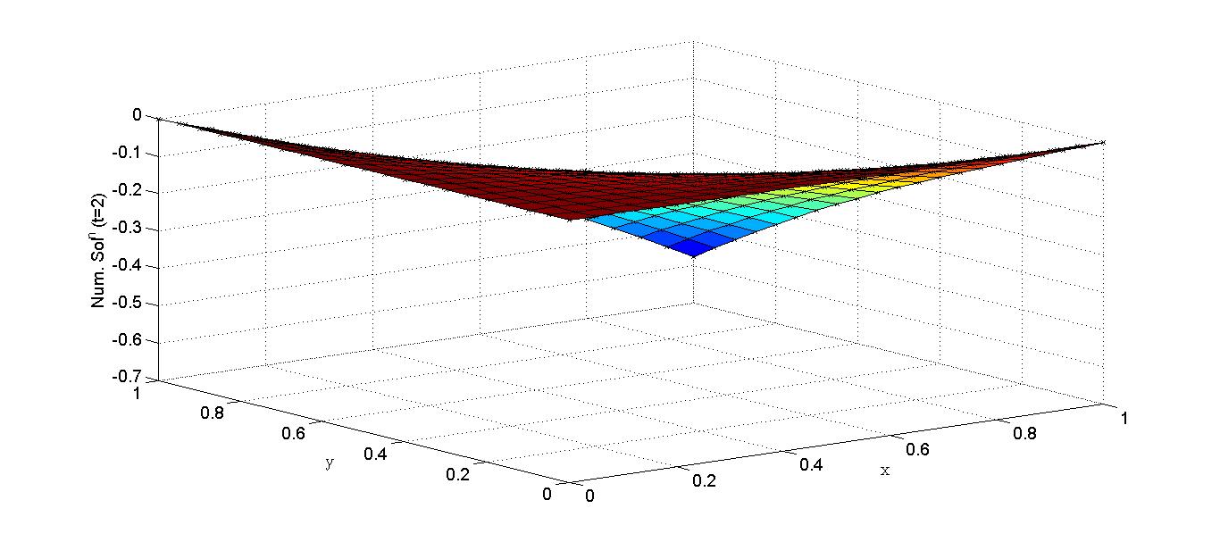
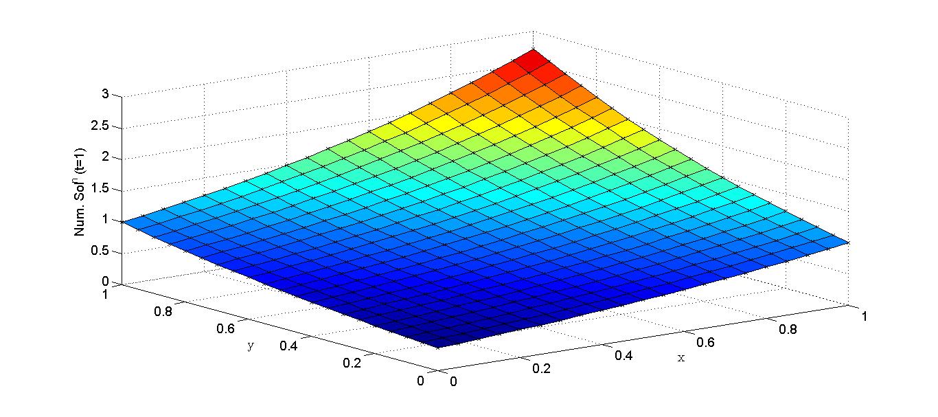
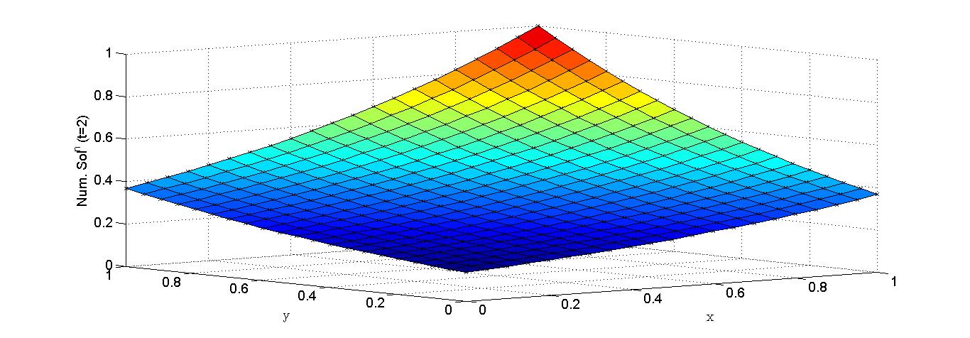
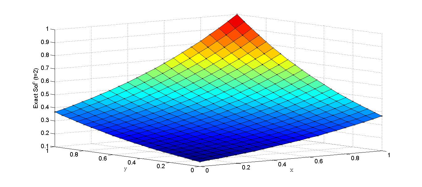
Example 2
Consider the telegraph equation (1) with , in ; for and for .
The exact solution [14] is given by
| (49) |
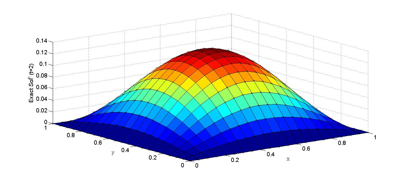
The solutions are computed for and with parameters , and . The computed error norms and CPU time for different time levels are compared with the error norms by Mittal and Bhatia [27] in Table 3, for and . In Table 4, the computed results for and are compared with Mittal and Bhatia [27] and Jiwari et al. [14]. The findings from the above tables confirms that the proposed results are better than [27, 14]. The CPU time is slightly more than [27] due to selection of SSP-RK54 scheme instead of SSP-RK43 scheme, for time integration. The surface plots of numerical and exact solutions at with and are depicted in Fig. 4.
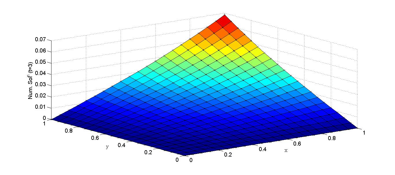
Example 3
Consider the telegraph equation (1) in the region with , and in , and for , and for
The exact solution [14] is given by
| (50) |
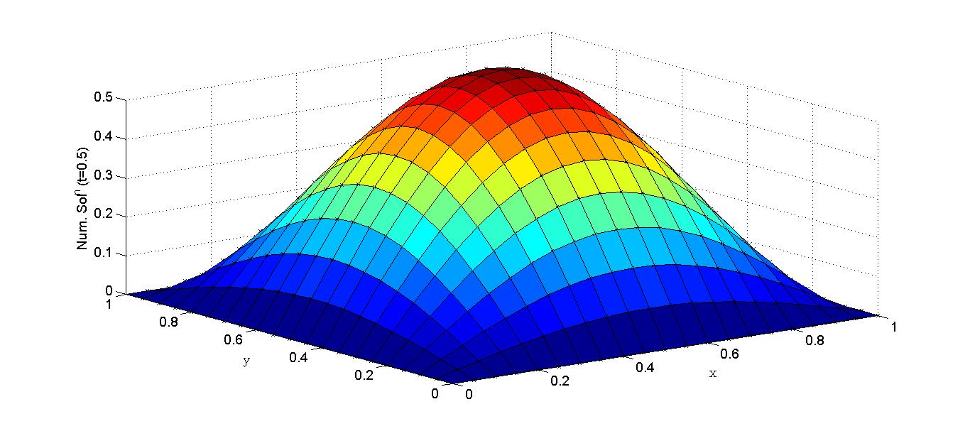
The solution is computed with the parameters and for the time step and The computed errors norms and CPU time at different time levels are reported in Table 5. It evident that our results are comparably better than the results by Bhatiya and Mittal[27]. A comparison of numerical solution with exact solution for is depicted in Fig. 5.
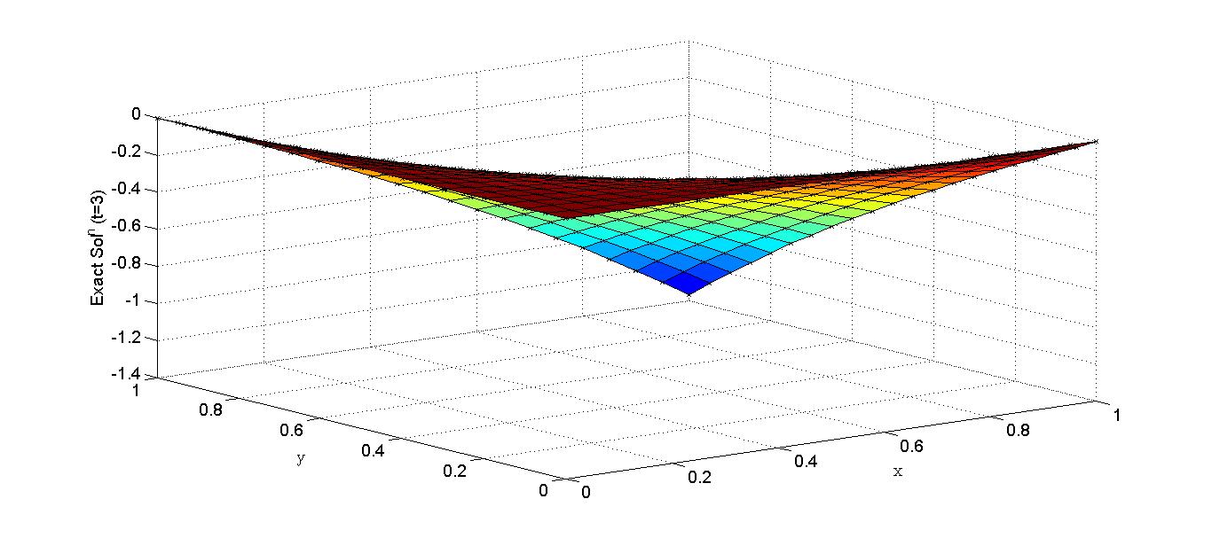
Example 4
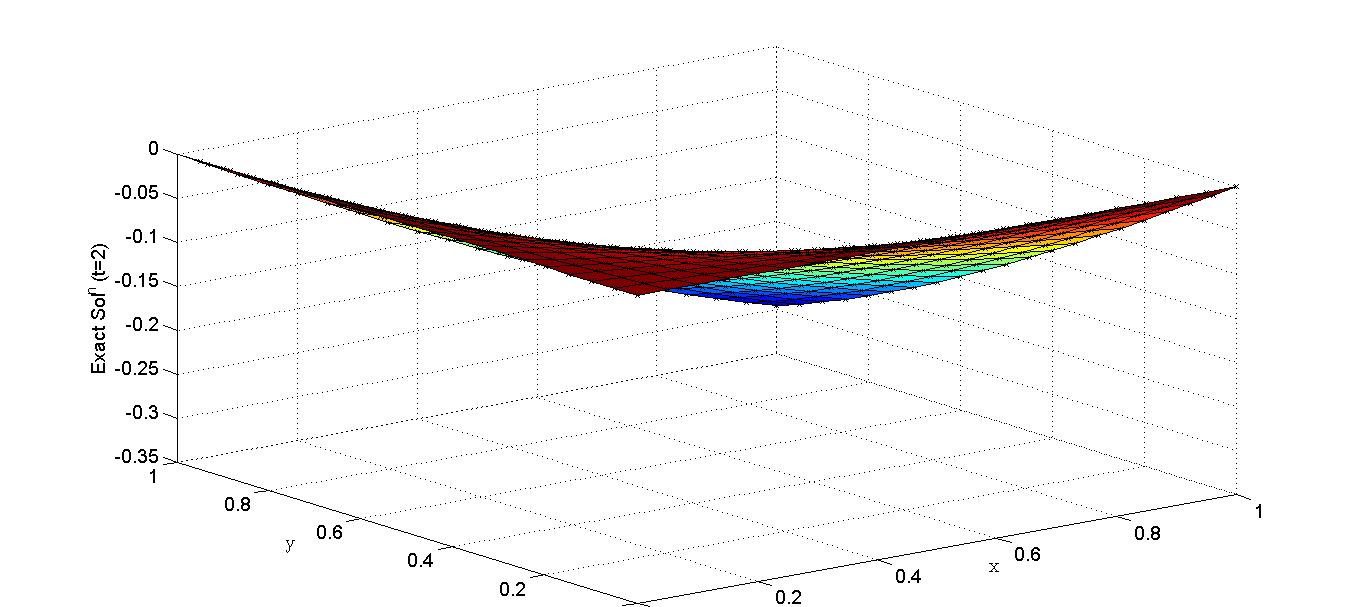
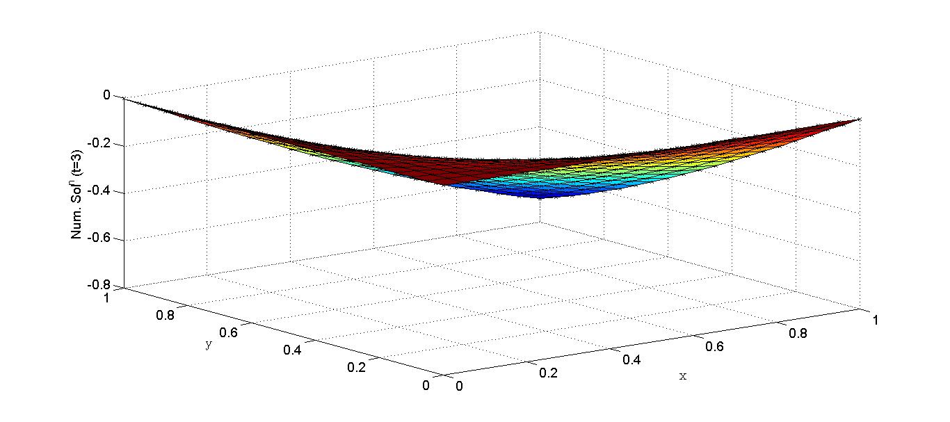
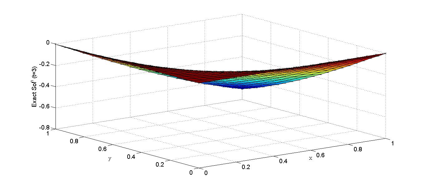
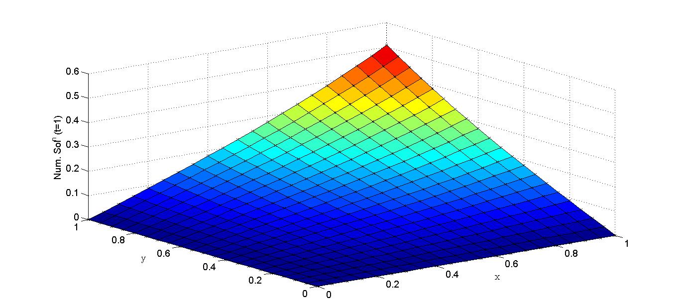
Consider the telegraph equation (1) in the region with , and in , and the mixed boundary conditions for and for The exact solution [2] is given by
| (51) |
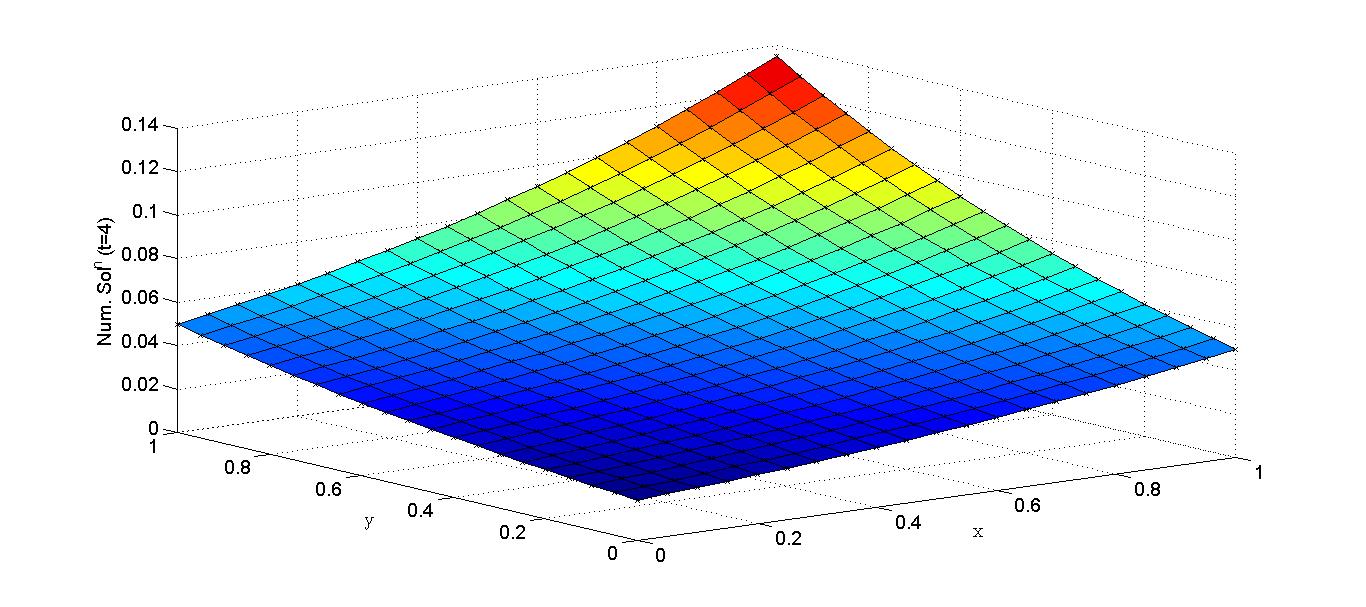
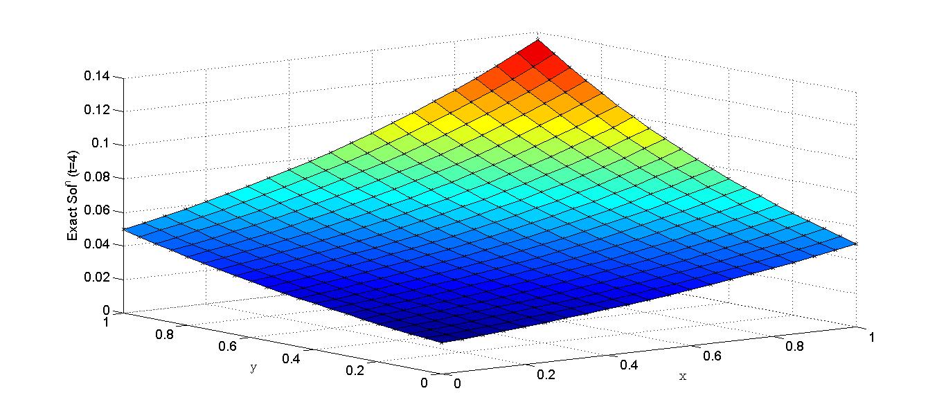
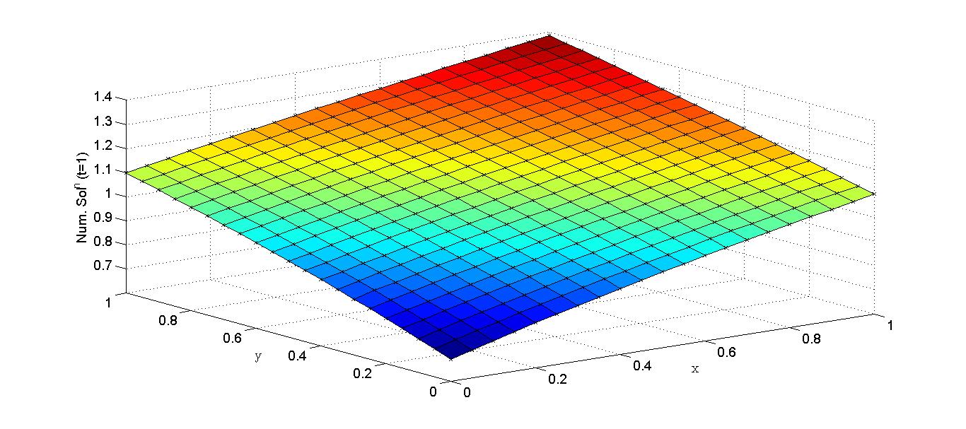
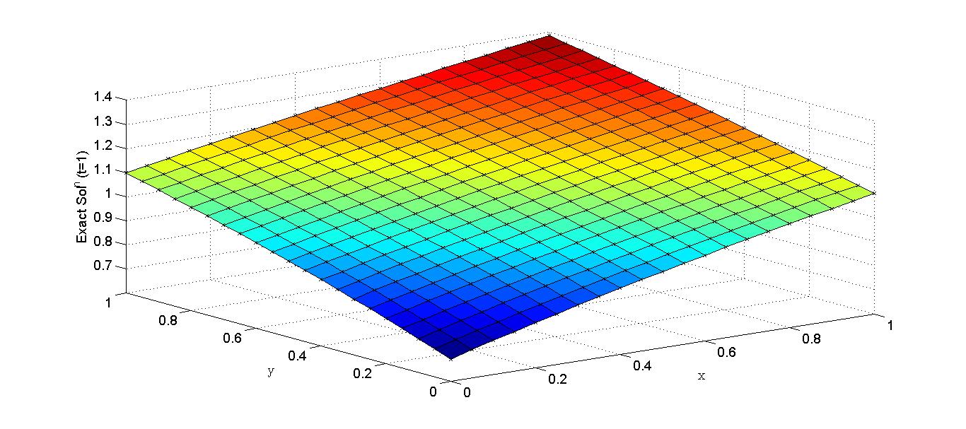
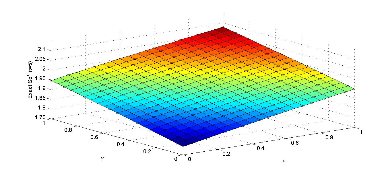
The computed results and CPU time are compared with the results by Mittal and Bhatia [27] for different space step size and time step size , and reported in Table 6 and Table 7. The surface plots of the mExp-DQM solutions and the exact solutions at different time levels is depicted in Fig. 6. It is evident accuracy of the proposed results is much better than results of Mittal and Bhatia [27].
Example 5
The telegraph equation (1) with , in region is considered together with in , and the mixed boundary conditions in and in The exact solution as in [2] is given by
| (52) |
The solutions are computed in terms of error norms, for and with and reported in Table 9 and Table 8. The surface plots of numerical and exact solutions at different time levels are depicted in Fig. 7. The above findings confirms that the proposed mExp-DQM solutions are more accurate as compared to the results by Mittal and Bhatia [27].
Example 6
The telegraph equation (1) with is considered together with in , and the mixed boundary conditions for and for The exact solution as given in [2] is:
| (53) |
where the function can be extracted from the exact solution.
The solution is computed for , in the region in terms of and relative error norms. The computed results are compared with the results by Mittal and Bhatia [27] and Dehghan and Ghesmati [12], reported in Table 10. It is evident from Table 10 that the accuracy of mExp-DQM results is much better than the accuracy in the results of [27], and [12] for large . The surface plots of numerical and exact solutions at different time levels are depicted in Fig. 8.
6 Conclusion
In this paper, we have developed a new differential quadrature method based on modified exponential cubic B-splines as a set of basis functions, and so, we called it modified exponential cubic B-spline differential quadrature method (mExp-DQM). The developed mExp-DQM with SSP-RK54 scheme is implemented for second order hyperbolic telegraph equation in dimension subject to initial conditions, and each type of boundary conditions: Drichlet, Neumann, mixed boundary conditions.
The results are compared with the recent results by Mittal and Bhatia [27] and Jiwari et al. [14]. It is evident that the accuracy of propped results is good as compared to very recent and accurate results due to [27, 14]. The CPU time is more than [27], while very less in comparison to [14]. Finally, we conclude that the proposed mExp-DQM results with suitable value of free parameter produces comparatively good results than [27, 14].
Acknowledgement
Pramod Kumar would like to thanks BBA University Lucknow, India for financial assistance to carry out the research work.
References
- [1] M. Lakestani, B.N. Saray, Numerical solution of telegraph equation using interpolating scaling functions, Comput. Math. Appl. 60 (7) (2010) 1964–1972.
- [2] M. Dehghan, A. Ghesmati, Solution of the second-order one-dimensional hyperbolic telegraph equation by using the dual reciprocity boundary integral equation (DRBIE) method, Eng. Anal. Bound. Elem. 34 (1) (2010) 51–59.
- [3] D M Pozar, Microwave Engineering, Addison-Wesley, 1990.
- [4] B. Bülbül, M. Sezer, Taylor polynomial solution of hyperbolic type partial differential equations with constant coefficients, Int. J. Comput. Math. 88 (3) (2011) 533–544.
- [5] F. Gao, C. Chi, Unconditionally stable difference schemes for a one-space-dimensional linear hyperbolic equation, Appl. Math. Comput. 187 (2) (2007) 1272–1276.
- [6] R.C. Mittal, R. Bhatia, Numerical solution of second order one dimensional hyperbolic telegraph equation by cubic B-spline collocation method, Appl. Math. Comput. 220 (2013) 496–506.
- [7] A. Saadatmandi, M. Dehghan, Numerical solution of hyperbolic telegraph equation using the Chebyshev tau method, Numer. Methods Partial Differ. Equ. 26 (1) (2010) 239–252.
- [8] R.K. Mohanty, New unconditionally stable difference schemes for the solution of multi–dimensional telegraphic equations, Int. J. Comput. Math. 86 (12) (2009) 2061–2071.
- [9] M. Dehghan, S.A. Yousefi, A. Lotfi, The use of He’s variational iteration method for solving the telegraph and fractional telegraph equations, Int. J. Numer. Methods Biomed. Eng. 27 (2) (2011) 219–231.
- [10] S. Sharifi, J. Rashidinia, Numerical solution of hyperbolic telegraph equation by cubic B-spline collocation method, Applied Mathematics and Computation 281 (2016) 28-38.
- [11] B. Bülbül, M. Sezer, A Taylor matrix method for the solution of a two-dimensional linear hyperbolic equation, Appl. Math. Lett. 24 (10) (2011) 1716-1720.
- [12] M. Dehghan, A. Ghesmati, Combination of meshless local weak and strong (MLWS) forms to solve the two dimensional hyperbolic telegraph equation, Eng. Anal. Bound. Elem. 34 (4) (2010) 324–336.
- [13] M. Dehghan, A. Mohebbi, High order implicit collocation method for the solution of two-dimensional linear hyperbolic equation, Numer. Methods Partial Differ. Equ. 25 (1) (2009) 232–243.
- [14] R. Jiwari, S. Pandit, R.C. Mittal, A differential quadrature algorithm to solve the two dimensional linear hyperbolic telegraph equation with Dirichlet and Neumann boundary conditions, Appl. Math. Comput. 218 (13) (2012) 7279–7294.
- [15] M. Dehghan, R. Salehi, A method based on meshless approach for the numerical solution of the two-space dimensional hyperbolic telegraph equation, Math. Methods Appl. Sci. 35 (10) (2012) 1220-1233.
- [16] H. Ding, Y. Zhang, A new fourth-order compact finite difference scheme for the two-dimensional second-order hyperbolic equation, J. Comput. Appl. Math. 230 (2) (2009) 626-632.
- [17] M. Dehghan, A. Shokri, A meshless method for numerical solution of a linear hyperbolic equation with variable coefficients in two space dimensions, Numer. Methods Partial Differ. Equ. 25 (2) (2009) 494-506.
- [18] R.K. Mohanty, M.K. Jain, An unconditionally stable alternating direction implicit scheme for the two space dimensional linear hyperbolic equation, Numer. Methods Partial Differ. Equ. 17 (6) (2001) 684-688.
- [19] Ozlem Ersoy and Idris Dag, Numerical solutions of the reaction diffusion system by using exponential cubic B-spline collocation algorithms, Open Phys. 13(2015)414-427.
- [20] R. Bellman, B. Kashef, E.S. Lee, R. Vasudevan, Solving hard problems by easy methods: differential and integral quadrature, Comput. Math. Appl. 1 (1) (1975) 133-143.
- [21] R. Bellman, B.G. Kashef, J. Casti, Differential quadrature: a technique for the rapid solution of nonlinear partial differential equations, J. Comput. Phys. 10 (1972) 40-52.
- [22] J.R. Quan, C.T. Chang, New insights in solving distributed system equations by the quadrature method-II, Comput. Chem. Eng. 13 (9) (1989) 1017-1024.
- [23] J.R. Quan, C.T. Chang, New insights in solving distributed system equations by the quadrature method-I, Comput. Chem. Eng. 13 (7) (1989) 779-788.
- [24] A. Korkmaz, I. Dag, Cubic B-spline differential quadrature methods and stability for Burgers’ equation, Eng. Comput. Int. J. Comput. Aided Eng. Software 30 (3) (2013) 320-344.
- [25] A. Korkmaz, I. Dag, Numerical simulations of boundary - forced RLW equation with cubic B-spline-based differential quadrature methods, Arab J Sci Eng 38 (2013) 1151-1160.
- [26] G. Arora, B. K. Singh, Numerical solution of Burgers’ equation with modified cubic B-spline differential quadrature method. Applied Math. Comput. 224 (2013) 166-177.
- [27] R.C. Mittal, Rachna Bhatia, A numerical study of two dimensional hyperbolic telegraph equation by modified B-spline differential quadrature method, Applied Mathematics and Computation 244 (2014) 976–997.
- [28] C. Shu, Y.T. Chew, Fourier expansion - based differential quadrature and its application to Helmholtz eigenvalue problems, Commun. Numer. Methods Eng. 13 (8) (1997) 643-653.
- [29] C. Shu, H. Xue, Explicit computation of weighting coefficients in the harmonic differential quadrature J. Sound Vib. 204(3) (1997) 549-555.
- [30] A.G. Striz, X. Wang, C.W. Bert, Harmonic differential quadrature method and applications to analysis of structural components, Acta Mech. 111 (1-2)(1995) 85-94.
- [31] A. Korkmaz, I. Dag, Shock wave simulations using sinc differential quadrature method, Eng. Comput. Int. J. Comput. Aided Eng. Software 28 (6) (2011) 654-674.
- [32] C. Shu, B. E. Richards, Application of generalized differential quadrature to solve two dimensional incompressible navier-Stokes equations, Int. J. Numer. Meth.Fluids 15 (1992) 791-798.
- [33] A. Korkmaz, A.M. Aksoy, I. Dag, Quartic B-spline differential quadrature method, Int. J. Nonlinear Sci. 11 (4) (2011) 403-411.
- [34] A. Korkmaz, I. Dag, Polynomial based differential quadrature method for numerical solution of nonlinear Burgers’ equation, J. Franklin Inst. 348 (10) (2011) 2863- 2875.
- [35] A. Korkmaz. Numerical algorithms for solutions of Kortewegde Vries equation. Numerical methods for partial differential equations, 26(6) (2010) 1504-1521.
- [36] A. Bashan, S. B. G. Karakoc, T. Geyikli, Approximation of the KdVB equation by the quintic B-spline differential quadrature method. Kuwait J. Sci. 42 (2) (2015) 67-92.
- [37] A. Korkmaz, I. Dag, Quartic and quintic Bspline methods for advection diffusion equation. Applied Mathematics and Computation 274 (2016) 208-219.
- [38] A. Korkmaz, and H. K. Akmaz, Numerical Simulations for Transport of Conservative Pollutants. Selcuk Journal of Applied Mathematics 16(1) (2015).
- [39] A. Korkmaz and H.K. Akmaz, Extended B-spline Differential Quadrature Method for Nonlinear Viscous Burgers’ Equation, Proceedings of International Conference on Mathematics and Mathematics Education, pp 323-323, Elaziǧ, Turkey 12-14 May, 2016.
- [40] W. Lee, Tridiagonal matrices: Thomas algorithm, Scientific Computation, University of Limerick, .
- [41] S. Gottlieb, D. I. Ketcheson, C. W. Shu, High Order Strong Stability Preserving Time Discretizations, J. Sci. Comput. 38 (2009) 251-289.
- [42] J. R. Spiteri, S. J. Ruuth, A new class of optimal high-order strong stability-preserving time-stepping schemes, SIAM J. Numer.Analysis 40 (2) (2002) 469–491.
- [43] M.K. Jain, Numerical Solution of Differential Equations, 2nd ed., Wiley, New York, NY, 1983.
- [44] Ethan J. Kubatko, Benjamin A. Yeager, David I. Ketcheson, Optimal strong-stability-preserving Runge-Kutta time discretizations for discontinuous Galerkin methods, http://www.davidketcheson.info/assets/papers/dg-ssp-stability.pdf.
7 List of Tables and Figures
| mExp-DQM | Mittal Bhatia [27] | ||||||||
|---|---|---|---|---|---|---|---|---|---|
| 1 | 3.7330E-06 | 4.5492E-06 | 2.7069E-04 | 0.031 | 9.9722E-04 | 2.2746E-03 | 5.9762E-03 | 0.08 | |
| 2 | 4.4842E-06 | 5.6294E-06 | 4.2217E-04 | 0.062 | 1.0926E-03 | 2.8706E-03 | 8.5019E-03 | 0.11 | |
| 3 | 3.7742E-06 | 6.3374E-06 | 1.4916E-04 | 0.109 | 2.2877E-04 | 6.0818E-04 | 7.4720E-04 | 0.14 | |
| 5 | 4.4186E-06 | 5.3912E-06 | 5.9036E-04 | 0.203 | 1.1562E-03 | 2.9942E-03 | 1.2767E-03 | 0.20 | |
| 7 | 3.2109E-06 | 3.7239E-06 | 1.6834E-04 | 0.312 | 7.2867E-04 | 1.8781E-03 | 3.1572E-03 | 0.26 | |
| 10 | 3.1806E-06 | 3.7506E-06 | 1.4949E-04 | 0.374 | 5.8889E-04 | 1.5158E-03 | 2.2874E-03 | 0.34 | |
| mExp-DQM (p=1) | mExp-DQM (p=0.15) | Mittal and Bhatia [27] | ||||||||||||
|---|---|---|---|---|---|---|---|---|---|---|---|---|---|---|
| CPU(s) | CPU (s) | CPU(s) | ||||||||||||
| 1 | 3.5715E-07 | 5.8718E-07 | 5.0162E-05 | 2.26 | 3.5729E-07 | 5.8736E-07 | 5.0182E-05 | 2.26 | 9.8870E-05 | 2.4964E-04 | 6.2977E-04 | 0.78 | ||
| 2 | 4.4969E-07 | 6.7211E-07 | 8.1823E-05 | 4.52 | 4.4977E-07 | 6.7225E-07 | 8.1838E-05 | 4.52 | 1.2148E-04 | 3.2296E-04 | 1.0025E-03 | 1.30 | ||
| 3 | 7.8128E-07 | 1.2228E-06 | 5.9879E-05 | 6.79 | 7.8151E-07 | 1.2231E-06 | 5.9897E-05 | 6.79 | 3.7627E-05 | 9.9310E-05 | 1.3078E-04 | 1.70 | ||
| 5 | 3.6743E-07 | 4.4790E-07 | 9.8297E-05 | 11.17 | 3.6749E-07 | 4.4797E-07 | 9.8311E-05 | 11.17 | 1.2762E-04 | 3.3205E-04 | 1.5411E-03 | 3.00 | ||
| 7 | 5.0400E-07 | 8.8032E-07 | 5.0732E-05 | 15.81 | 5.0417E-07 | 8.8056E-07 | 5.0749E-05 | 15.81 | 6.7672E-05 | 1.7679E-04 | 3.0892E-04 | 3.30 | ||
| 10 | 5.7992E-07 | 9.9151E-07 | 5.2483E-05 | 22.60 | 5.8011E-07 | 9.9178E-07 | 5.2500E-05 | 22.60 | 5.1764E-05 | 1.3521E-04 | 2.1245E-04 | 5.20 | ||
| Mittal and Bhatia [27] | mECDQ method | ||||||||
|---|---|---|---|---|---|---|---|---|---|
| 0.5 | 8.3931E-04 | 3.3019E-03 | 2.8902E-03 | 0.13 | 6.8998E-06 | 1.0168E-05 | 2.8749E-04 | 0.016 | |
| 1 | 6.0254E-04 | 2.0597E-03 | 3.4208E-03 | 0.16 | 5.3522E-06 | 7.0133E-06 | 3.6767E-04 | 0.046 | |
| 2 | 2.4167E-04 | 7.6531E-04 | 3.7297E-03 | 0.19 | 2.2337E-06 | 2.8534E-06 | 4.1711E-04 | 0.078 | |
| 3 | 8.9534E-05 | 2.7920E-04 | 3.7937E-03 | 0.24 | 8.3375E-07 | 1.0585E-06 | 4.2747E-04 | 0.141 | |
| 5 | 1.2168E-05 | 3.7800E-05 | 3.8097E-03 | 0.34 | 1.1352E-07 | 1.4389E-07 | 4.3005E-04 | 0.218 | |
| mECDQ method | Mittal and Bhatia [27] | Jiwari et al. [14] | ||||||||||
|---|---|---|---|---|---|---|---|---|---|---|---|---|
| CPU(s) | CPU(s) | CPU(s) | ||||||||||
| 0.5 | 8.1273E-07 | 1.3152E-06 | 6.6847E-05 | 1.279 | 1.0690E-04 | 2.4738E-04 | 1.1088E-04 | 0.47 | 1.1185E-04 | 6 | ||
| 1 | 5.8429E-07 | 8.3976E-07 | 7.9233E-05 | 2.496 | 1.5293E-05 | 3.3082E-04 | 1.3266E-04 | 1.10 | 1.8051E-04 | 12 | ||
| 2 | 2.3507E-07 | 3.2200E-07 | 8.6737E-05 | 5.896 | 4.6468E-05 | 1.1380E-05 | 3.1954E-04 | 1.10 | 4.7289E-04 | 25 | ||
| 3 | 8.8032E-08 | 1.1937E-07 | 8.8297E-05 | 7.488 | 2.1994E-05 | 4.3577E-05 | 1.3024E-04 | 2.80 | 1.2656E-04 | 37 | ||
| 5 | 1.1979E-08 | 1.6202E-08 | 8.8694E-05 | 12.402 | 2.7151E-06 | 5.4141E-06 | 1.4439E-04 | 4.30 | 9.2770E-04 | 62 | ||
| 0.5 | 7.2898E-07 | 9.0815E-07 | 5.9958E-05 | 1.279 | 9.2959E-05 | 4.2348E-04 | 3.4675E-04 | 0.52 | 1.1198E-04 | 6 | ||
| 1 | 8.0739E-07 | 1.0270E-06 | 1.0949E-04 | 2.511 | 6.3652E-05 | 2.5838E-04 | 3.9146E-04 | 0.98 | 1.8635E-04 | 12 | ||
| 2 | 5.7525E-07 | 7.2622E-07 | 2.1226E-04 | 5.007 | 2.5540E-05 | 9.5843E-05 | 4.2739E-04 | 1.80 | 5.1797E-04 | 25 | ||
| 3 | 3.1155E-07 | 3.9340E-07 | 3.1248E-04 | 7.394 | 9.9234E-06 | 3.5340E-05 | 4.5140E-04 | 2.20 | 1.4412E-04 | 37 | ||
| 5 | 6.7799E-08 | 8.5767E-08 | 5.0198E-04 | 12.470 | 1.5116E-06 | 4.8043E-06 | 5.0758E-04 | 4.50 | 1.0883E-04 | 62 | ||
| mECDQ method | Mittal and Bhatia [27] | |||||||||
|---|---|---|---|---|---|---|---|---|---|---|
| CPU(s) | CPU(s) | CPU(s) | ||||||||
| 0.5 | 2.0862E-06 | 2.8531E-06 | 1.294 | 2.0861E-06 | 2.8527E-06 | 1.310 | 1.070E-04 | 3.756E-04 | 0.57 | |
| 1 | 2.5046E-06 | 3.2481E-06 | 2.62 | 2.5045E-06 | 3.2479E-06 | 2.608 | 1.717E-04 | 5.640E-04 | 0.92 | |
| 2 | 1.3896E-06 | 1.7942E-06 | 6.115 | 1.3896E-06 | 1.7942E-06 | 5.179 | 1.647E-04 | 5.130E-04 | 1.20 | |
| 3 | 1.4008E-06 | 2.2256E-06 | 7.722 | 1.4006E-06 | 2.2252E-06 | 7.722 | 8.986E-06 | 1.956E-05 | 2.30 | |
| 5 | 1.6566E-06 | 2.1478E-06 | 12.885 | 1.6566E-06 | 2.1478E-06 | 12.901 | 1.774E-04 | 5.563E-04 | 4.10 | |
| 7 | 2.5344E-06 | 3.2884E-06 | 18.142 | 2.5342E-06 | 3.2882E-06 | 18.008 | 1.420E-04 | 4.723E-04 | 5.40 | |
| 10 | 1.8983E-06 | 2.4641E-06 | 25.631 | 1.8983E-06 | 2.4640E-06 | 25.646 | 1.224E-04 | 4.122E-04 | 7.40 | |
| 0.5 | 2.2128E-06 | 3.2835E-06 | 1.544 | 2.2127E-06 | 3.2833E-06 | 1.294 | 9.880E-05 | 3.696E-04 | 0.57 | |
| 1 | 3.2434E-06 | 4.4892E-06 | 2.574 | 3.2433E-06 | 4.4891E-06 | 2.605 | 1.677E-04 | 5.687E-04 | 0.94 | |
| 2 | 2.4069E-06 | 3.2575E-06 | 5.194 | 2.4069E-06 | 3.2575E-06 | 5.179 | 1.711E-04 | 5.257E-04 | 1.40 | |
| 3 | 1.6269E-06 | 2.8366E-06 | 7.800 | 1.6267E-06 | 2.8362E-06 | 7.769 | 1.741E-05 | 4.346E-05 | 2.50 | |
| 5 | 3.1532E-06 | 4.2934E-06 | 13.182 | 3.1531E-06 | 4.2933E-06 | 13.104 | 1.842E-04 | 5.694E-04 | 4.10 | |
| 7 | 3.5801E-06 | 5.1314E-06 | 18.19 | 3.5799E-06 | 5.1312E-06 | 18.018 | 1.376E-04 | 4.759E-04 | 6.00 | |
| 10 | 3.3621E-06 | 4.8638E-06 | 20.748 | 3.3620E-06 | 4.8635E-06 | 26.198 | 1.1691E-04 | 4.1396E-04 | 8.80 | |
| mExp-DQM | Mittal and Bhatia [27] | ||||||
|---|---|---|---|---|---|---|---|
| CPU(s) | CPU(s) | ||||||
| 1 | 3.9796E-04 | 6.7076E-04 | 0.031 | 1.4441E-02 | 2.9996E-02 | 0.03 | |
| 2 | 4.5099E-05 | 1.1091E-04 | 0.063 | 1.3898E-03 | 3.9711E-03 | 0.05 | |
| 3 | 4.0589E-05 | 7.4545E-05 | 0.109 | 1.3018E-03 | 2.2178E-03 | 0.08 | |
| 5 | 4.1078E-06 | 8.6460E-06 | 0.187 | 1.1112E-04 | 2.0618E-04 | 0.11 | |
| 7 | 4.6749E-07 | 1.0452E-06 | 0.234 | 1.3695E-05 | 3.0052E-05 | 0.14 | |
| 10 | 3.8692E-08 | 7.0454E-08 | 0.312 | 1.4408E-06 | 2.5354E-06 | 0.19 | |
| mExp-DQM | Mittal and Bhatia [27] | ||||||
|---|---|---|---|---|---|---|---|
| CPU(s) | CPU(s) | ||||||
| 0.5 | 1.28E-04 | 2.67E-04 | 1.045 | 3.4808E-03 | 9.5129E-03 | 0.50 | |
| 1 | 1.05E-04 | 1.82E-04 | 2.074 | 3.2351E-03 | 7.4749E-03 | 0.70 | |
| 2 | 1.04E-05 | 3.07E-05 | 4.181 | 2.8518E-04 | 1.0361E-03 | 1.30 | |
| 3 | 1.09E-05 | 2.05E-05 | 6.255 | 3.1028E-04 | 5.7859E-04 | 1.90 | |
| 5 | 1.03E-06 | 2.40E-06 | 10.358 | 2.4495E-05 | 6.7234E-05 | 3.30 | |
| 7 | 1.03E-07 | 2.59E-07 | 14.446 | 2.5376E-06 | 8.2203E-06 | 3.90 | |
| 10 | 1.18E-08 | 2.18E-08 | 20.498 | 3.6505E-06 | 8.5897E-06 | 5.20 | |
| mExp-DQM () | Mittal and Bhatia [27] | ||||||||
|---|---|---|---|---|---|---|---|---|---|
| CPU(s) | CPU(s) | ||||||||
| 1 | 5.7365E-04 | 7.1586E-04 | 5.7365E-04 | 7.1591E-04 | 0.05 | 1.6144E-03 | 3.6006E-03 | 0.07 | |
| 2 | 1.7371E-04 | 2.2392E-04 | 1.7372E-04 | 2.2396E-04 | 0.11 | 2.6345E-03 | 5.7068E-03 | 0.09 | |
| 3 | 1.9296E-05 | 2.1468E-05 | 1.9298E-05 | 2.1476E-05 | 0.14 | 5.3845E-04 | 1.2479E-03 | 0.11 | |
| 5 | 6.4893E-06 | 8.5658E-06 | 6.4900E-06 | 8.5675E-06 | 0.25 | 1.2418E-04 | 2.1003E-04 | 0.15 | |
| 7 | 1.3028E-06 | 1.6270E-06 | 1.3028E-06 | 1.6272E-06 | 0.33 | 1.3653E-05 | 2.6261E-05 | 0.12 | |
| 10 | 5.8266E-08 | 7.3567E-08 | 5.8266E-08 | 7.3573E-08 | 0.45 | 7.5592E-06 | 1.4083E-06 | 0.20 | |
| mExp-DDQM (p=0.5, 1) | Mittal and Bhatia [27] | ||||||||
|---|---|---|---|---|---|---|---|---|---|
| CPU(s) | CPU(s) | ||||||||
| 0.5 | 3.2617E-05 | 4.6301E-05 | 3.2617E-05 | 4.6306E-05 | 1.33 | 3.5833E-04 | 9.5129E-04 | 0.3 | |
| 1 | 5.5100E-05 | 7.2237E-05 | 5.5100E-05 | 7.2239E-05 | 2.54 | 3.2351E-04 | 7.4749E-04 | 0.7 | |
| 2 | 1.5539E-05 | 2.1379E-05 | 1.5539E-05 | 2.1380E-05 | 5.09 | 2.8518E-05 | 1.0361E-04 | 1.3 | |
| 3 | 8.3598E-07 | 1.1501E-06 | 8.3602E-07 | 1.1504E-06 | 7.61 | 3.1028E-05 | 5.7859E-04 | 1.7 | |
| 5 | 5.1811E-07 | 7.4769E-07 | 5.1812E-07 | 7.4772E-07 | 12.81 | 2.4495E-06 | 6.7234E-05 | 2.9 | |
| 7 | 1.5582E-07 | 1.9983E-07 | 1.5582E-07 | 1.9983E-07 | 17.78 | 2.5376E-07 | 8.2203E-07 | 4.1 | |
| 10 | 7.1281E-09 | 9.0990E-09 | 7.1281E-09 | 9.0991E-09 | 25.80 | 3.6505E-09 | 8.5897E-08 | 5.4 | |
| mExp-DQM | Mittal and Bhatia [27] | Dehghan and Ghesmati [12] | ||||||||||||
|---|---|---|---|---|---|---|---|---|---|---|---|---|---|---|
| CPU (s) | CPU (s) | MLWS | CPU (s) | MLPG | CPU (s) | |||||||||
| 0.5 | 4.795E-05 | 9.727E-05 | 1.097E-03 | 1.05 | 1.069E-03 | 2.474E-03 | 1.109E-03 | 0.5 | 7.939E-05 | 9.2 | 9.991E-05 | 21.0 | ||
| 1 | 7.290E-05 | 1.081E-04 | 1.394E-03 | 2.18 | 1.529E-03 | 3.308E-03 | 1.327E-03 | 1.1 | 9.098E-05 | 12.9 | 7.198E-05 | 36.2 | ||
| 2 | 2.946E-05 | 4.931E-05 | 4.466E-04 | 4.23 | 4.647E-04 | 1.138E-03 | 3.195E-04 | 2.0 | 8.705E-04 | 25.7 | 8.784E-05 | 49.1 | ||
| 3 | 1.200E-05 | 2.086E-05 | 1.567E-04 | 6.28 | 2.199E-04 | 4.358E-04 | 1.302E-04 | 2.8 | 9.931E-04 | 38.1 | 4.801E-04 | 66.8 | ||
| 4 | 1.281E-05 | 1.948E-05 | 1.502E-04 | 8.46 | 2.715E-04 | 5.414E-04 | 1.444E-05 | 4.3 | 4.703E-03 | 49.8 | 6.091E-04 | 82.0 | ||
| 5 | 7.989E-06 | 1.247E-05 | 8.626E-05 | 10.49 | 1.720E-04 | 3.481E-04 | 8.423E-05 | 7.0 | 7.302E-03 | 62.0 | 9.498E-04 | 97.3 | ||
| 10 | 2.738E-06 | 4.198E-06 | 2.314E-05 | 21.00 | 7.729E-05 | 1.404E-04 | 2.962E-05 | 9.6 | ||||||